Shear stresses of colloidal dispersions at the glass transition in equilibrium and in flow

Abstract

We consider a model dense colloidal dispersion at the glass transition, and investigate the connection between equilibrium stress fluctuations, seen in linear shear moduli, and the shear stresses under strong flow conditions far from equilibrium, viz. flow curves for finite shear rates. To this purpose thermosensitive core-shell particles consisting of a polystyrene core and a crosslinked poly(N-isopropylacrylamide)(PNIPAM) shell were synthesized. Data over an extended range in shear rates and frequencies are compared to theoretical results from integrations through transients and mode coupling approaches. The connection between non-linear rheology and glass transition is clarified. While the theoretical models semi-quantitatively fit the data taken in fluid states and the predominant elastic response of glass, a yet unaccounted dissipative mechanism is identified in glassy states.

I Introduction

Complex fluids and soft materials in general are characterized by a strong variability in their rheological and elastic properties under flow and deformations.Larson Within the linear response framework, storage- and loss- (shear) moduli describe elastic contributions in solids and dissipative processes in fluids. Both moduli are connected via Kramers-Kronig relations and result from Fourier-transformations of a single time-dependent function, the shear modulus $g^{\rm lr}(t)$. Importantly, the linear response modulus $g^{\rm lr}(t)$ itself is defined in the quiescent system and (only) describes the small shear-stress fluctuations always present in thermal equilibrium.Larson ; russel

Viscoelastic materials exhibit both, elastic and dissipative, phenomena depending on external control parameters like temperature and/ or density. The origins of the change between fluid and solid like behavior can be manifold, including phase transitions of various kinds. One mechanism existent quite universally in dense systems is the glass transition, that structural rearrangements of particles become progressively slower.Goe:92 It is accompanied by a structural relaxation time which grows dramatically. Maxwell was the first to describe this fluid-solid transition phenomenologically. Dispersions consisting of colloidal, slightly polydisperse (near) hard spheres arguably constitute one of the most simple viscoelastic systems, where a glass transition has been identified. It has been studied in detail by dynamic light scattering measurements,Pus:87 ; Meg:91 ; Meg:93 ; Meg:94 ; Heb:97 ; Bec:99 ; Bar:02 ; Eck:03 confocal microscopy,Wee:00 linear,Mas:95 ; Zac:06 and non-linear rheology.Sen:99 ; Sen:99b ; Pet:99 ; Pet:02 ; Pet:02b ; Pha:06 ; Bes:07 ; Cra:06 Computer simulations are available also.Phu:96 ; Str:99 ; Dol:00 Mode coupling theory (MCT) has provided a semi-quantitative explanation of the observed glass transition phenomena, albeit neglecting ageing effects Pur:06 and decay processes at ultra-long times that may cause (any) colloidal glass to flow ultimately.Goe:91 ; Goe:92 ; Goe:99 Importantly, MCT predicts a purely kinetic glass transition and describes it using only equilibrium structural input, namely the equilibrium structure factor $S_{q}$russel ; dhont measuring thermal density fluctuations.

The stationary, nonlinear rheological behavior under steady shearing provides additional insight into the physics of dense colloidal dispersions.Larson ; russel A priori it is not clear, whether the mechanisms relevant during glass formation also dominate the nonlinear rheology. Solvent mediated interactions (hydrodynamic interactions), which do not affect the equilibrium phase diagram, may become crucially important. Also, shear may cause ordering or layering of the particles.Lau:92 Simple phenomenological relations between the frequency dependence of the linear response and the shear rate dependence of the nonlinear response, like the Cox-Merz rule, have been formulated, but often lack firm theoretical support or are limited to special shear histories.Larson ; Wys:07

On the other hand, within a number of theoretical approaches a connection between steady state rheology and the glass transition has been suggested. Brady worked out a scaling description of the rheology based on the concept that the structural relaxation arrests at random close packing.Bra:93 In the soft glassy rheology model, the trap model of glassy relaxation by Bouchaud was generalized to describe mechanical deformations and ageing.Sol:97 ; Sol:98 ; Fie:00 The mean field approach to spin glasses was generalized to systems with broken detailed balance in order to model flow curves of glasses under shear.Ber:00 ; Ber:02 The application of these novel approaches to colloidal dispersions has lead to numerous insights, but has been hindered by the use of unknown parameters in the approaches. MCT, also, was generalized to include effects of shear,Miy:02 ; miyazaki ; Kob:05 and, within the integrations through transients (ITT) approach, to quantitatively describe all aspects of stationary states under steady shearing.Fuc:02 ; Fuc:03 ; Fuc:05c Some aspects of the ITT approach to flow curves have already been tested,Cra:06 ; Var:06 but the connection, central in the approach, between fluctuations around equilibrium and the nonlinear response, has not been investigated experimentally up to now.

In the present contribution we explore the connection between structural relaxation close to glassy arrest and the rheological properties far from equilibrium. Thereby we crucially test the ITT approach, which aims to unify the understanding of these phenomena. It requires, as sole input, information on the equilibrium structure (namely $S_{q}$), and, first gives a formally exact generalization of the shear modulus to finite shear rates, $g(t,\dot{\gamma})$, which is then approximated in a consistent way. We investigate a model dense colloidal dispersion at the glass transition, and determine its linear and nonlinear rheology. Thermosensitive core-shell particles consisting of a polystyrene core and a crosslinked poly(N-isopropylacrylamide)(PNIPAM) shell were synthesized and their dispersions characterized in detail.Cra:06 ; Cra:07 Data over an extended range in shear rates and frequencies are compared to theoretical results from MCT and ITT.

The paper is organized as follows: section II summarizes the equations of the microscopic ITT approach in order to provide a self-contained presentation of the theoretical framework. In section III some of the universal predictions of ITT are discussed in order to describe the phenomenological properties of the non-equilibrium transition studied in this work. Building on the universal properties, section IV introduces a simplified model which reproduces the phenomenology. Section V introduces the experimental system. Section VI contains the main part of the present work, the comparison of combined measurements of the linear and non-linear rheology of the model dispersion with calculations in microscopic and simplified theoretical models. A short summary concludes the paper, while the appendix presents an extension of the simplified model used in the main text.

II Microscopic approach

We consider $N$ spherical particles with radius $R_{H}$ dispersed in a volume $V$ of solvent (viscosity $\eta_{s}$) with imposed homogeneous, and constant linear shear-flow. The flow velocity points along the $x$-axis and its gradient along the $y$-axis. The motion of the particles (with positions ${\bf r}_{i}(t)$ for $i=1,\ldots,N$) is described by $N$ coupled Langevin equationsdhont

$$\zeta\left(\frac{d{\bf r}_{i}}{dt}-{\bf v}^{\rm solv}({\bf r}_{i})\right)={\bf F}_{i}+{\bf f}_{i}\;.$$ (1)

Solvent friction is measured by the Stokes friction coefficient $\zeta=6\pi\eta_{s}R_{H}$. The $N$ vectors ${\bf F}_{i}=-\partial/\partial{\bf r}_{i}\,U(\left\{{\bf r}_{j}\right\})$ denote the interparticle force on particle $i$ deriving from potential interactions with all other particles; $U$ is the potential energy which depends on all particles’ positions. The solvent shear-flow is given by ${\bf v}^{\rm solv}({\bf r})=\dot{\gamma}\,y\,\hat{\bf x}$, and the Gaussian white noise force satisfies (with $\alpha,\beta$ denoting directions)

$$\langle f^{\alpha}_{i}(t)\;f^{\beta}_{j}(t^{\prime})\rangle=2\zeta\,k_{B}T\,\delta_{\alpha\beta}\,\delta_{ij}\,\delta(t-t^{\prime})\;,$$

where $k_{B}T$ is the thermal energy. Each particle experiences interparticle forces, solvent friction, and random kicks. Interaction and friction forces on each particle balance on average, so that the particles are at rest in the solvent on average. The Stokesian friction is proportional to the particle’s motion relative to the solvent flow at its position; the latter varies linearly with $y$. The random force on the level of each particle satisfies the fluctuation dissipation relation.

An important approximation in Eq. (1) is the neglect of hydrodynamic interactions, which would arise from the proper treatment of the solvent flow around moving particles.russel ; dhont In the following we will argue that such effects can be neglected at high densities where interparticle forces hinder and/or prevent structural rearrangements, and where the system is close to arrest into an amorphous, metastable solid. Another important approximation in Eq. (1) is the assumption of a given, constant shear rate $\dot{\gamma}$, which does not vary throughout the (infinite) system. We start with this assumption in the philosophy that, first, homogeneous states should be considered, before heterogeneities and confinement effects are taken into account. All difficulties in Eq. (1) thus are connected to the many-body interactions given by the forces ${\bf F}_{i}$, which couple the $N$ Langevin equations. In the absence of interactions, ${\bf F}_{i}\equiv 0$, Eq. (1) leads to super-diffusive particle motion termed ’Taylor dispersion’.dhont

While formulation of the considered microscopic model handily uses Langevin equations, theoretical analysis proceeds more easily from the reformulation of Eq. (1) as Smoluchowski equation. It describes the temporal evolution of the distribution function $\Psi(\left\{{\bf r}_{i}\right\},t)$ of the particle positions

$$\partial_{t}\Psi(\left\{{\bf r}_{i}\right\},t)=\Omega\;\Psi(\left\{{\bf r}_{i}\right\},t)\;,$$ (2)

employing the Smoluchowski operator,russel ; dhont

$$\Omega=\sum_{j=1}^{N}\left[D_{0}\;\frac{\partial}{\partial{\bf r}_{j}}\cdot\left(\frac{\partial}{\partial{\bf r}_{j}}-\frac{1}{k_{B}T}\,{\bf F}_{j}\right)-\dot{\gamma}\,\frac{\partial}{\partial x_{j}}\,y_{j}\right]\;,$$ (3)

built with the (bare) diffusion coefficient $D_{0}=k_{B}T/\zeta$ of a single particle. We assume that the system relaxes into a unique stationary state at long times, so that $\Psi(t\to\infty)=\Psi_{s}$ holds. Homogeneous, amorphous systems are studied so that the stationary distribution function $\Psi_{s}$ is translationally invariant but anisotropic. Neglecting ageing, the formal solution of the Smoluchowski equation within the ITT approach can be brought into the formFuc:02 ; Fuc:05c

$$\Psi_{s}=\Psi_{e}+\frac{\dot{\gamma}}{k_{B}T}\;\int_{0}^{\infty}\!\!\!\!dt\;\Psi_{e}\;\sigma_{xy}\;e^{\Omega^{\dagger}t}\;,$$ (4)

where the adjoint Smoluchowski $\Omega^{\dagger}$ operator arises from partial integrations. It acts on the quantities to be averaged with $\Psi_{s}$. $\Psi_{e}$ denotes the equilibrum canonical distribution function, $\Psi_{e}\propto e^{-U/(k_{B}T)}$, which is the time-independent solution of Eq. (2) for $\dot{\gamma}=0$; in Eq. (4), it gives the initial distribution at the start of shearing (at $t=0$). The potential part of the stress tensor $\sigma_{xy}=-\sum_{i=1}^{N}F^{x}_{i}\,y_{i}$ entered via $\Omega\Psi_{e}=\dot{\gamma}\,\sigma_{xy}\,\Psi_{e}$. The simple, exact result Eq. (4) is central to the ITT approach as it connects steady state properties to time integrals formed with the shear-dependent dynamics. The latter contains slow intrinsic particle motion.

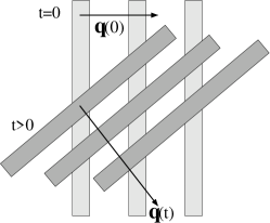
Figure 1: Shear advection of a fluctuation with initial wavevector in $x$-direction, ${\bf q}(t\!\!=\!\!0)=q\,(1,0,0)^{T}$, and advected wavevector at later time ${\bf q}(t\!\!>\!\!0)=q\,(1,-\dot{\gamma}t,0)^{T}$. At all times, ${\bf q}(t)$ is perpendicular to the planes of constant fluctuation amplitude. Note that the magnitude $q(t)=q\sqrt{1+(\dot{\gamma}t)^{2}}$ increases with time. Brownian motion, neglected in this sketch, would smear out the fluctuation.

In ITT, the evolution towards the stationary distribution at infinite times is approximated by following the slow structural rearrangements, encoded in the transient density correlator $\Phi_{\bf q}(t)$. It is defined byFuc:02 ; Fuc:05c

$$\Phi_{\bf q}(t)=\frac{1}{NS_{q}}\;\langle\,\delta\varrho^{*}_{{\bf q}}\;e^{\Omega^{\dagger}t}\;\delta\varrho_{{\bf q}(t)}\,\rangle^{(\dot{\gamma}=0)}\;.$$ (5)

It describes the fate of an equilibrium density fluctuation with wavevector ${\bf q}$, where $\varrho_{\bf q}=\sum_{j=1}^{N}e^{i{\bf q}\cdot{\bf r}_{j}}$, under the combined effect of internal forces, Brownian motion and shearing. Note that because of the appearance of $\Psi_{e}$ in Eq. (4), the average in Eq. (5) can be evaluated with the equilibrium canonical distribution function, while the dynamical evolution contains Brownian motion and shear advection. The normalization is given by $S_{q}$ the equilibrium structure factor russel ; dhont for wavevector modulus $q=|{\bf q}|$. The advected wavevector enters in Eq. (5)

$${\bf q}(t)={\bf q}-\dot{\gamma}t\;q_{x}\;\hat{\bf y}\;,$$ (6)

where unit-vector $\hat{\bf y}$ points in $y$-direction) The time-dependence in ${\bf q}(t)$ results from the affine particle motion with the shear flow of the solvent. Translational invariance under shear dictates that at a time $t$ later, the equilibrium density fluctuation $\delta\varrho^{*}_{\bf q}$ has a nonvanishing overlap only with the advected fluctuation $\delta\varrho_{{\bf q}(t)}$; see Fig. 1, where a non-decorrelating fluctuation is sketched under shear. In the case of vanishing Brownian motion, viz. $D_{0}=0$ in Eq. (3), we find $\Phi_{{\bf q}}(t)\equiv 1$, because the advected wavevector takes account of simple affine particle motion.achtung The relaxation of $\Phi_{{\bf q}}(t)$ thus heralds decay of structural correlations. Within ITT, the time integral over such structural decorrelations provides an approximation to the stationary state:

$$\Psi_{s} \approx \Psi_{e}+$$

$$\frac{\dot{\gamma}}{2k_{B}T}\int_{0}^{\infty}\!\!\!\!\!\!dt\sum_{\bf k}\frac{k_{x}k_{y}\,S^{\prime}_{k}}{k\,NS^{2}_{{\bf k}(t)}}\;\Phi^{2}_{{\bf k}}(t)\;\left(\Psi_{e}\,\varrho^{*}_{{\bf k}(t)}\,\varrho_{{\bf k}(t)}\right)\,,$$

with $S^{\prime}_{k}=\partial S_{k}/\partial k$.eq5com The last term in brackets in Eq. (II) expresses, that the expectation value of a general fluctuation $A$ in ITT-approximation contains the (equilibrium) overlap with the local structure, $\langle\varrho^{*}_{\bf k}\,\varrho_{\bf k}\,A\rangle^{(\dot{\gamma}=0)}$. The difference between the equilibrium and stationary distribution functions then follows from integrating over time the spatially resolved (viz. wavevector dependent) density variations.

The general results for $\Psi_{s}$, the exact one of Eq. (4) and the approximation Eq. (II), can be applied to compute stationary expectation values like for example the thermodynamic transverse stress, $\sigma(\dot{\gamma})=\langle\sigma_{xy}\rangle/V$. Equation (4) leads to an exact non-linear Green-Kubo relation:

$$\sigma(\dot{\gamma})=\dot{\gamma}\int_{0}^{\infty}dt\;g(t,\dot{\gamma})\;,$$ (8)

where the generalized shear modulus $g(t,\dot{\gamma})$ depends on shear rate via the Smoluchowski operator from Eq. (3)

$$g(t,\dot{\gamma})=\frac{1}{k_{B}TV}\;\langle\,\sigma_{xy}\;e^{\Omega^{\dagger}t}\;\sigma_{xy}\,\rangle^{(\dot{\gamma}=0)}\;.$$ (9)

In ITT, the slow stress fluctuations in $g(t,\dot{\gamma})$ are approximated by following the slow structural rearrangements, encoded in the transient density correlators. The generalized modulus becomes, using the approximation Eq. (II), or, equivalently, performing a mode coupling approximation:Fuc:03 ; Fuc:02 ; miyazaki

$$g(t,\dot{\gamma})=\frac{k_{B}T}{2}\,\int\!\!\frac{d^{3}k}{(2\pi)^{3}}\;\frac{k_{x}^{2}k_{y}k_{y}(t)}{k\,k(t)}\;\frac{S^{\prime}_{k}S^{\prime}_{k(t)}}{S^{2}_{k(t)}}\;\Phi^{2}_{{\bf k}}(t)\;,$$ (10)

Summation over wavevectors has been turned into integration in Eq. (10) considering an infinite system.

The familiar shear modulus of linear response theory describes thermodynamic stress fluctuations in equilibrium, and is obtained from Eqs. (9,10) by setting $\dot{\gamma}=0$.Larson ; russel ; Nae:98 While Eq. (9) then gives the exact Green-Kubo relation, the approximation Eq. (10) turns into the well-studied MCT formula. For finite shear rates, Eq. (10) describes how affine particle motion causes stress fluctuations to explore shorter and shorter length scales. There the effective forces, as measured by the gradient of the direct correlation function, $S^{\prime}_{k}/S_{k}^{2}=nc^{\prime}_{k}=n\partial c_{k}/\partial k$, become smaller, and vanish asympotically, $c^{\prime}_{k\to\infty}\to 0$; the direct correlation function $c_{k}$ is connected to the structure factor via the Ornstein-Zernicke equation $S_{k}=1/(1-n\,c_{k})$, where $n=N/V$ is the particle density. Note, that the equilibrium structure suffices to quantify the effective interactions, while shear just pushes the fluctuations around on the ’equilibrium energy landscape’.

Structural rearrangements of the dispersion affected by Brownian motion is encoded in the transient density correlator. Shear induced affine motion, viz.  the case $D_{0}=0$, is not sufficient to cause $\Phi_{\bf k}(t)$ to decay. Brownian motion of the quiescent correlator $\Phi^{(\dot{\gamma}=0)}_{k}(t)$ leads at high densities to a slow structural process which arrests at long times in (metastable) glass states. Thus the combination of structural relaxation and shear is interesting. The interplay between intrinsic structural motion and shearing in $\Phi_{\bf k}(t)$ is captured by $(i)$ first a formally exact Zwanzig-Mori type equation of motion, and $(ii)$ second a mode coupling factorisation in the memory function built with longitudinal stress fluctuations.Fuc:02 ; Fuc:05c The equation of motion for the transient density correlators is

$$\partial_{t}\Phi_{\bf q}(t)+\Gamma_{\bf q}(t)\;\left\{\Phi_{\bf q}(t)+\int_{0}^{t}dt^{\prime}\;m_{\bf q}(t,t^{\prime})\;\partial_{t^{\prime}}\,\Phi_{\bf q}(t^{\prime})\right\}=0\;,$$ (11)

where the initial decay rate $\Gamma_{\bf q}(t)=D_{0}\,q^{2}(t)/S_{q(t)}$ generalizes the familiar result from linear response theory to advected wavevectors; it contains Taylor dispersion. The memory equation contains fluctuating stresses and similarly like $g(t,\dot{\gamma})$ in Eq. (II), is calculated in mode coupling approximation

$$m_{\bf q}(t,t^{\prime})=\frac{1}{2N}\sum_{{\bf k}}V_{{\bf q}{\bf k}{\bf p}}(t,t^{\prime})\;\Phi_{{\bf k}(t^{\prime})}(t-t^{\prime})\;\Phi_{{\bf p}(t^{\prime})}(t-t^{\prime})\;,$$ (12)

where we abbreviated ${\bf p}={\bf q}-{\bf k}$. The vertex generalizes the expression in the quiescent case:Fuc:02

$$V_{{\bf q}{\bf k}{\bf p}}(t,t^{\prime}) = \frac{S_{{\bf q}(t)}\,S_{{\bf k}(t^{\prime})}\,S_{{\bf p}(t^{\prime})}}{q^{2}(t)\,q^{2}(t^{\prime})}\;{\cal V}_{{\bf q}{\bf k}{\bf p}}(t)\;{\cal V}_{{\bf q}{\bf k}{\bf p}}(t^{\prime})\,,$$

$${\cal V}_{{\bf q}{\bf k}{\bf p}}(t) = {\bf q}(t)\cdot\left(\,{\bf k}(t)\;nc_{k(t)}+{\bf p}(t)\;nc_{p(t)}\,\right)\;.$$ (13)

With shear, wavevectors in Eq. (II) are advected according to Eq. (6).

Equations (II,11,12), with the specific example of the generalized shear modulus Eq. (10), form a closed set of equations determining rheological properties of a sheared dispersion from equilibrium structural input.Fuc:02 ; Fuc:05c Only the static structure factor $S_{q}$ is required to predict $(i)$ the time dependent shear modulus within linear response, $g^{\rm lr}(t)=g(t,\dot{\gamma}=0)$, and $(ii)$ the stationary stress $\sigma(\dot{\gamma})$ from Eq. (8). The loss and storage moduli of small amplitude oscillatory shear measurementsLarson ; russel follow from Eq. (9) in the linear response case $(i)$

$$G^{\prime}(\omega)+i\,G^{\prime\prime}(\omega)=i\omega\;\int_{0}^{\infty}dt\;e^{-i\,\omega\,t}\;g(t,\dot{\gamma}=0)\;.$$ (14)

While, in the linear response regime, modulus and density correlator are measurable quantities, outside the linear regime, both quantities serve as tools in the ITT approach only. The transient correlator and shear modulus provide a route to the stationary averages, because they describe the decay of equilibrium fluctuations under external shear, and their time integral provides an approximation for the stationary distribution function, see Eq. (II). Determination of the frequency dependent moduli under large amplitude oscillatory shear has become possible recently only,Miy:06 and requires an extension of the present approach to time dependent shear rates in Eq. (3).Bra:07

III Universal aspects

The summarized microscopic ITT equations contain a bifurcation in the long-time behavior of $\Phi_{\bf q}(t)$, which corresponds to a non-equilibrium transition between a fluid and a shear-molten glassy state; it is described in this section. Close to the transition, (rather) universal predictions can be made about the non-linear dispersion rheology and the steady state properties. The central predictions are introduced in this section and summarized in the overview figure 2. It is obtained from the schematic model which is also used to analyse the data, and which is introduced in the following Sect. IV.

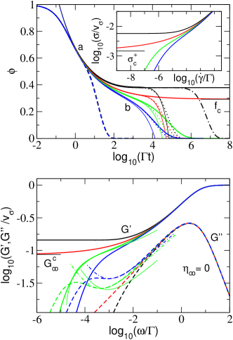
Figure 2: Overview of the properties of the F${}_{12}^{(\dot{\gamma})}$-model characteristic for the transition between fluid and yielding glass. The upper panel shows numerically obtained transient correlators $\Phi(t)$ for $\varepsilon=0.01$ (black curves), $\varepsilon=0$ (red), $\varepsilon=-0.005$ (green), and $\varepsilon=-0.01$ (blue). The shear rates are $\left|\dot{\gamma}/\Gamma\right|=0$ (thick solid lines), $\left|\dot{\gamma}/\Gamma\right|=10^{-6}$ (dotted lines), and $\left|\dot{\gamma}/\Gamma\right|=10^{-2}$ (dashed lines). For the glass state at $\varepsilon=0.01$ (black), $\left|\dot{\gamma}/\Gamma\right|=10^{-8}$ (dashed-dotted-line) is also included. All curves were calculated with $\gamma_{c}=0.1$ and $\eta_{\infty}=0$. The thin solid lines give the factorization result Eq. (15) with scaling functions $\cal G$ for $\left|\dot{\gamma}/\Gamma\right|=10^{-6}$; label $a$ marks the critical law (17), and label $b$ marks the von Schweidler-law (18). The critical glass form factor $f_{c}$ is indicated. The inset shows the flow curves for the same values for $\varepsilon$. The thin black bar shows the yield stress $\sigma^{+}_{c}$ for $\varepsilon=0$. The lower panel shows the viscoelastic storage (solid line) and loss (broken line modulus for the same values of $\varepsilon$. The thin green lines are the Fourier-transformed factorization result Eq. (15) with scaling function $\cal G$ taken from the upper panel for $\varepsilon=-0.005$. The dashed-dotted lines show the fit formula Eq. (29) for the spectrum in the minimum-region with $G_{\rm min}/v_{\sigma}=0.0262$, $\omega_{\rm min}/\Gamma=0.000457$ at $\varepsilon=-0.005$ (green) and $G_{\rm min}/v_{\sigma}=0.0370$, $\omega_{\rm min}/\Gamma=0.00105$ at $\varepsilon=-0.01$ (blue). The elastic constant at the transition $G_{\infty}^{c}$ is marked also, while the high frequency asymptote $G^{\prime}_{\infty}=G^{\prime}(\omega\to\infty)$ is not labeled explicitly.

A dimensionless separation parameter $\varepsilon$ measures the distance to the transition which is situated at $\varepsilon=0$. A fluid state ($\varepsilon<0$) possesses a (Newtonian) viscosity, $\eta_{0}(\varepsilon<0)=\lim_{\dot{\gamma}\to 0}\sigma(\dot{\gamma})/\dot{\gamma}$, and shows shear-thinning upon increasing $\dot{\gamma}$. Via the relation $\eta_{0}=\lim_{\omega\to 0}\,G^{\prime\prime}(\omega)/\omega$, the Newtonian viscosity can also be taken from the loss modulus at low frequencies, where $G^{\prime\prime}(\omega)$ dominates over the storage modulus. The latter varies like $G^{\prime}(\omega\to 0)\sim\omega^{2}$. A glass ($\varepsilon\geq 0$), in the absence of flow, possesses an elastic constant $G_{\infty}$, which can be measured in the elastic shear modulus $G^{\prime}(\omega)$ in the limit of low frequencies, $G^{\prime}(\omega\to 0,\varepsilon\geq 0)\to G_{\infty}(\varepsilon)$. Here the storage modulus dominates over the loss one, which drops like $G^{\prime\prime}(\omega\to 0)\sim\omega$. (Note that the high frequency modulus $G^{\prime}_{\infty}=G^{\prime}(\omega\to\infty)$ is characteristic of the particle interactions,Lio:94 and exists in fluid and solid states.) Enforcing steady shear flow melts the glass. The stationary stress of the shear-molten glass always exceeds a (dynamic) yield stress. For decreasing shear rate, the viscosity increases like $1/\dot{\gamma}$, and the stress levels off onto the yield-stress plateau, $\sigma(\dot{\gamma}\to 0,\varepsilon\geq 0)\to\sigma^{+}(\varepsilon)$.

Close to the transition, the zero-shear viscosity $\eta_{0}$, the elastic constant $G_{\infty}$, and the yield stress $\sigma^{+}$ show universal anomalies as functions of the distance to the transition: the viscosity diverges in a power-law $\eta_{0}(\varepsilon\to 0-)\sim(-\varepsilon)^{-\gamma}$ with material dependent exponent $\gamma$ around $2-3$, the elastic constant increases like a square-root $G_{\infty}(\varepsilon\to 0+)-G_{\infty}^{c}\sim\sqrt{\varepsilon}$, and the dynamic yield stress $\sigma^{+}(\varepsilon\to 0+)$ also increases with infinite slope above its value $\sigma^{+}_{c}$ at the bifurcation. The quantities $G_{\infty}^{c}$ and $\sigma^{+}_{c}$ denote the respective values at the transition point $\varepsilon=0$, and measure the jump in the elastic constant and in the yield stress at the glass transition; in the fluid state, $G_{\infty}(\varepsilon<0)=0$ and $\sigma^{+}(\varepsilon<0)=0$ hold.

The described results follow from the stability analysis of Eqs. (11,12) around an arrested, glassy structure $f_{q}$ of the transient correlator.Fuc:02 ; Fuc:03 Considering the time window where $\Phi_{\bf q}(t)$ is metastable and close to arrest at $f_{q}$, and taking all control parameters like density, temperature, etc. to be close to the values at the transition, the stability analysis yields the ’factorization’ between spatial and temporal dependences

$$\Phi_{\bf q}(t)=f^{c}_{q}+h_{q}\;{\cal G}(\,t/t_{0},\varepsilon,\dot{\gamma}t_{0}\,)+\ldots\;,$$ (15)

where the (isotropic) glass form factor $f^{c}_{q}$ and critical amplitude $h_{q}$ describe the spatial properties of the metastable glassy state. The critical glass form factor $f^{c}_{q}$ gives the long-lived component of density fluctuations, and $h_{q}$ captures local particle rearrangements. Both can be taken as constants independent on shear rate and density, as they are evaluated from the vertices in Eq. (II) at the transition point. All time-dependence and (sensitive) dependence on the external control parameters is contained in the function $\cal G$, which often is called ’$\beta$-correlator’ and obeys the non-linear stability equation

$$\varepsilon-c^{(\dot{\gamma})}\;(\dot{\gamma}t)^{2}+\lambda\;{\cal G}^{2}(t)=\frac{d}{dt}\int_{0}^{t}\!\!\!dt^{\prime}\;{\cal G}(t-t^{\prime})\;{\cal G}(t^{\prime})\;,$$ (16)

with initial condition

$${\cal G}(t\to 0)\to(t/t_{0})^{-a}\;.$$ (17)

The two parameters $\lambda$ and $c^{(\dot{\gamma})}$ in Eq. (16) are determined by the static structure factor at the transition point, and take values around $\lambda\approx 0.73$ and $c^{(\dot{\gamma})}\approx 3$ for $S_{q}$ taken from Percus-Yevick approximationrussel for hard sphere interactions.Fuc:02 ; Fuc:03 ; ishsm The transition point then lies at packing fraction $\phi_{c}=\frac{4\pi}{3}n_{c}R_{H}^{3}\approx 0.52$ (index $c$ for critical), and the separation parameter measures the relative distance, $\varepsilon=C\,(\phi-\phi_{c})/\phi_{c}$ with $C\approx 1.3$. The ’critical’ exponent $a$ is given by the exponent parameter $\lambda$ via $\lambda=\Gamma(1-a)^{2}/\Gamma(1-2a)$.Goe:91 ; Goe:92

The time scale $t_{0}$ in Eq. (17) provides the means to match the function ${\cal G}(t)$ to the microscopic, short-time dynamics. The Eqs. (11,12) contain a simplified description of the short time dynamics in colloidal dispersions via the initial decay rate $\Gamma_{\bf q}(t)$. From this model for the short-time dynamics, the time scale $t_{0}\approx 1.6\,10^{-2}R_{H}^{2}/D_{0}$ is obtained. Solvent mediated effects on the short time dynamics are well known and are neglected in $\Gamma_{\bf q}(t)$ in Eq. (11). Within the ITT approach, one finds that if hydrodynamic interactions were included in Eq. (11), all of the mentioned universal predictions would remain true. Only the value of $t_{0}$ will be shifted and depend on the short time hydrodynamic interactions. For the quiescent glass transition this has been discussed within MCT,Fra:98 and ITT extends this to driven cases. This statement remains valid in ITT, as long as the hydrodynamic interactions do not affect the mode coupling vertex in Eq. (II). In this sense, hydrodynamic interactions can be incorporated into the theory of the glass transition, and amount to a rescaling of the matching time $t_{0}$, only.

Obviously, the matching time $t_{0}$ also provides an upper cut-off for the time window of the structural relaxation. At times shorter than $t_{0}$ the specific short-time dynamics matters. The condition $\dot{\gamma}t_{0}\ll 1$ follows and translates into a restriction for the accessible range of shear rates, $\dot{\gamma}\ll\dot{\gamma}_{*}$, where the upper-cut off shear rate $\dot{\gamma}_{*}$ is connected to the matching time.

The parameters $\varepsilon$, $\lambda$ and $c^{(\dot{\gamma})}$ in Eq. (16) can be determined from the equilibrium structure factor $S_{q}$ at or close to the transition, and, together with $t_{0}$ and the shear rate $\dot{\gamma}$ they capture the essence of the rheological anomalies in dense dispersions. A divergent viscosity follows from the prediction of a strongly increasing final relaxation time in $\cal G$ in the quiescent fluid phase

$${\cal G}(t\to\infty,\varepsilon<0,\dot{\gamma}=0)\to-\left(t/\tau\right)^{b}\quad,\;\;\mbox{with }\;\frac{t_{0}}{\tau}\propto(-\varepsilon)^{\gamma}\;.$$ (18)

The entailed temporal power law, termed von Schweidler law, initiates the final decay of the correlators, which has a density and temperature independent shape $\tilde{\Phi}_{q}(\tilde{t})$. The final decay, often termed $\alpha$-relaxation, depends on $\varepsilon$ only via the time scale $\tau(\varepsilon)$ which rescales the time, $\tilde{t}=t/\tau$. Equation (16) establishes the crucial time scale separation between $t_{0}$ and $\tau$, the divergence of $\tau$, and the stretching (non-exponentiality) of the final decay; it also gives the values of the exponents via $\lambda=\Gamma(1+b)^{2}/\Gamma(1+2b)$, and $\gamma=(1/a+1/b)/2$. Using Eq. (10), the divergence of the Newtonian viscosity follows.Goe:92 ; Goe:91 During the final decay the shear modulus becomes a function of rescaled time, $\tilde{g}(\tilde{t}=t/\tau,\dot{\gamma}=0)$, leading to $\eta_{0}\propto\tau(\varepsilon)$; its initial value is given by the elastic constant at the transition, $\tilde{g}(\tilde{t}\ll 1,\varepsilon\to 0-,\dot{\gamma}=0)=G_{\infty}^{c}$.

On the glassy side of the transition, $\varepsilon\geq 0$, the transient density fluctuations stays close to a plateau value for intermediate times which increases when going deeper into the glass,

$${\cal G}(t_{0}\ll t\ll 1/|\dot{\gamma}|,\varepsilon\geq 0)\to\sqrt{\frac{\varepsilon}{1-\lambda}}+{\cal O}(\varepsilon)\;.$$ (19)

Entered into Eq. (10), the square-root dependence of the plateau value translates into the square-root anomaly of the elastic constant $G_{\infty}$, and causes the increase of the yield stress close to the glass transition.

Only, for vanishing shear rate, $\dot{\gamma}=0$, an ideal glass state exists in the ITT approach for steady shearing. All density correlators arrest at a long time limit, which from Eq. (19) close to the transition is given by $\Phi_{\bf q}(t\to\infty,\varepsilon\geq 0,\dot{\gamma}=0)=f_{q}=f^{c}_{q}+h_{q}\sqrt{\varepsilon/(1-\lambda)}+{\cal O}(\varepsilon)$. Consequently the modulus remains elastic at long times, $g(t\to\infty,\varepsilon\geq 0,\dot{\gamma}=0)=G_{\infty}>0$. Any (infinitesimal) shear rate, however, melts the glass and causes a final decay of the transient correlators. The function $\cal G$ initiates the decay around the critical plateau of the transient correlators and sets the common time scale for the final decay under shear

$${\cal G}(t\to\infty,\varepsilon\geq 0)\to-\sqrt{\frac{c^{(\dot{\gamma})}}{\lambda-\frac{1}{2}}}\;|\dot{\gamma}t|\;.$$ (20)

Under shear all correlators decay from the plateau as function of $|\dot{\gamma}t|$. Steady shearing thus prevents non-ergodic arrest and restores ergodicity. This aspect of Eq. (16) has two important ramifications for the steady state of shear molten glasses.Fuc:02 ; Fuc:03 First, ITT finds that shear melts a glass and produces a unique steady state at long times. This conclusion is restricted by the assumption of homogeneous states and excludes the possible existence of ordering or layering under shear. Also, ageing was neglected, which could remain because of non-ergodicity in the initial quiescent state. (Ergodicity of the sheared state however suggests ageing to be unimportant under shear.Ber:00 ; Fie:00 ) Second, all stationary averages, which in ITT are obtained from integrating up the transient fluctuations, do not exhibit a linear response regime in the glass. Rather they take finite values for vanishing shear rate, which jump discontinuously at the glass transition. This holds because the shear-driven decay of Eq. (20) initiates a scaling law where the transient correlators decay as function of $|\dot{\gamma}t|$ down from the plateau $f_{q}$ to zero, denoted as $\Phi^{+}_{\bf q}(t|\dot{\gamma}|)$. When entered into Eq. (II), time appears only in the combination together with shear rate and thus after time integration the shear rate dependence drops out, yielding a finite result even in the limit of infinitesimal shear rate. Prominent example of a stationary average that has no linear response regime with respect to $\dot{\gamma}$ in the glass phase is the shear stress $\sigma(\dot{\gamma},\varepsilon\geq 0)$. It takes finite values for vanishing shear rate, $\sigma^{+}(\varepsilon)=\sigma(\dot{\gamma}\to 0,\varepsilon\geq 0)$, and jumps at the glass transition from zero to a finite value. Because of Eq. (19) it increases rapidly when moving deeper into the glass.

IV Schematic model

The universal aspects described in the previous section are contained in any ITT model that contains the central bifurcation scenario and recovers Eqs. (15,16). Equation (15) states that spatial and temporal dependences decouple in the intermediate time window. Thus it is possible to investigate ITT models without proper spatial resolution. Because of the technical difficulty to evaluate the anisotropic functionals in Eqs. (10,12), it is useful to restrict the description to few or to a single transient correlator. In the schematic $F_{12}^{(\dot{\gamma})}$-model,Fuc:03 a single ’typical’ density correlator $\Phi(t)$, conveniently normalized according to $\Phi(t\to 0)=1-\Gamma t$, obeys a Zwanzig-Mori memory equation which is modeled according to Eq. (11)

$$\partial_{t}\Phi(t)+\Gamma\left\{\Phi(t)+\int_{0}^{t}dt^{\prime}\;m(t-t^{\prime})\;\partial_{t^{\prime}}\Phi(t^{\prime})\right\}=0\;.$$ (21)

The parameter $\Gamma$ mimics the microscopic dynamics of the ’typical’ density correlator chosen in Eq. (21), and will depend on structural and hydrodynamic correlations. The memory function describes stress fluctuations which become more sluggish together with density fluctuations, because slow structural rearrangements dominate all quantities. A self consistent approximation closing the equations of motion is made mimicking Eq. (12). In the $F_{12}^{(\dot{\gamma})}$-model one includes a linear term (absent in Eq. (12)) in order to $(i)$ sweep out the full range of $\lambda$ values in Eq. (16), and $(ii)$ retain algebraic simplicity:

$$m(t)=\frac{v_{1}\,\Phi(t)+v_{2}\,\Phi^{2}(t)}{1+\left(\dot{\gamma}t/\gamma_{c}\right)^{2}}$$ (22)

This model, for the quiescent case $\dot{\gamma}=0$, had been suggested by Götze in 1984,Goe:84 ; Goe:91 and describes the development of slow structural relaxation upon increasing the coupling vertices $v_{i}\geq 0$; they mimic the dependence of the vertices in Eq. (12) at $\dot{\gamma}=0$ on the equilibrium structure given by $S_{q}$. Under shear an explicit time dependence of the couplings in $m(t)$ captures the accelerated loss of memory by shear advection in Eq. (12). Shearing causes the dynamics to decay for long times, because fluctuations are advected to smaller wavelengths where small scale Brownian motion relaxes them. Equations (21,22) lead, with $\Phi(t)=f^{c}+(1-f^{c})^{2}\,{\cal G}(t,\varepsilon,\dot{\gamma})$, and the choice of the vertices $v_{2}=v_{2}^{c}=2$, and $v_{1}=v_{1}^{c}+\varepsilon\,(1-f^{c})/f^{c}$, where $v_{1}^{c}=0.828$, to the critical glass form factor $f^{c}=0.293$ and to the stability equation (16), with parameters

$$\lambda=0.707\,,\;c^{(\dot{\gamma})}=0.586/\gamma_{c}^{2}\,\mbox{, and }\;t_{0}=0.426/\Gamma\;.$$

The choice of transition point $(v_{1}^{c},v_{2}^{c})$ is motivated by its repeated use in the literature. Actually, there is a line of glass transitions where the long time limit $f=\Phi(t\to\infty)$ jumps discontinuously. It is parameterized by $(v_{1}^{c},v_{2}^{c})=((2\lambda-1),1)/\lambda^{2}$ with $0.5\leq\lambda<1$, and $f^{c}=1-\lambda$. The present choice is just a typical one, which corresponds to the given typical $\lambda$-value. The separation parameter $\varepsilon$ is the crucial control parameter as it takes the system through the transition. The parameter $\gamma_{c}$ is a scale for the magnitude of strain that is required in order for the accumulated strain $\dot{\gamma}t$ to matter.erweiterung In Eq. (16), it is connected to the parameter $c^{(\dot{\gamma})}$ .

For simplicity, the quadratic dependence of the generalized shear modulus on density fluctuations is retained from the microscopic Eq. (10). It simplifies because only one density mode is considered, and as, for simplicity, a possible dependence of the vertex (prefactor) $v_{\sigma}$ on shear is neglected

$$g(t)=v_{\sigma}\,\Phi^{2}(t)+\eta_{\infty}\;\delta(t)\;.$$ (23)

The parameter $\eta_{\infty}$ characterizes a short-time, high frequency viscosity and models viscous processes which require no structural relaxation. Together with $\Gamma$ (respectively $t_{0}$), it is the only model parameter affected by solvent mediated interactions. Steady state shear stress under constant shearing, and viscosity then follow via integrating up the generalized modulus:

$$\sigma=\eta\;\dot{\gamma}=\dot{\gamma}\;\int_{0}^{\infty}\!\!\!dt\;g(t)=\dot{\gamma}\;\int_{0}^{\infty}\!\!\!dt\;v_{\sigma}\Phi^{2}(t)+\dot{\gamma}\;\eta_{\infty}\;.$$ (24)

Also, when setting shear rate $\dot{\gamma}=0$ in Eqs. (21,22), so that the schematic correlator belongs to the quiescent, equilibrium system, the frequency dependent moduli are obtained from Fourier transforming:

$$G^{\prime}(\omega)+i\,G^{\prime\prime}(\omega)=i\,\omega\,\int_{0}^{\infty}dt\;e^{-i\,\omega\,t}\;v_{\sigma}\left.\Phi^{2}(t)\right|_{\dot{\gamma}=0}+i\omega\,\eta_{\infty}\;.$$ (25)

Because of the vanishing of the Fourier-integral in Eq. (25) for high frequencies, the parameter $\eta_{\infty}$ can be identified as high frequency viscosity:

$$\lim_{\omega\to\infty}G^{\prime\prime}(\omega)/\omega=\eta^{\omega}_{\infty}\quad,\;\mbox{with }\;\eta^{\omega}_{\infty}=\eta_{\infty}\;.$$ (26)

At high shear, on the other hand, Eq. (22) leads to a vanishing of $m(t)$, and Eq. (21) gives an exponential decay of the transient correlator, $\Phi(t)\to e^{-\Gamma\,t}$ for $\dot{\gamma}\to 0$. The high shear viscosity thus becomes

$$\eta^{\dot{\gamma}}_{\infty}=\lim_{\dot{\gamma}\to\infty}\sigma(\dot{\gamma})/\dot{\gamma}=\eta_{\infty}+\frac{v_{\sigma}}{2\,\Gamma}=\eta^{\omega}_{\infty}+\frac{v_{\sigma}}{2\,\Gamma}\;.$$ (27)

Representative solutions of the F${}_{12}^{(\dot{\gamma})}$-model are summarized in Fig.2, which bring out the discussed universal aspects included in all ITT models.

V Experimental system and methods

The particles consist of a solid core of poly(styrene) onto which a network of crosslinked poly(N-isopropylacrylamide) (PNIPAM) is affixed. The degree of crosslinking of the PNIPAM shell effected by the crosslinker N,N’-methylenebisacrylamide (BIS) was 5 Mol $\%$. The core-shell type PS-NIPAM particles were synthesized, purified and characterized as described in ref.Din:98 Immersed in water the shell swells at low temperatures. Raising the temperature above 32^oC leads to a volume transition within the shell. To investigate the structure and swelling of the particles cryogenic transmission electron microscopy and dynamic light scattering have been used.

Screening the remaining electrostatic interactions by adding 5.10^-2 molL^-1 KCl, the system crystallises as hard spheres.Cra:06 Experimental details on the characterization of the particles and on the determination of the effective volume are given elsewhere.Cra:07 The dependence of $\phi_{\rm eff}$ on the temperature is given by the hydrodynamic radius $R_{H}$ determined from the dynamic light scattering in the dilute regime. $R_{H}$ was linearly extrapolated between 14 and 25^oC ($R_{H}=-0.85925T+123.78$ with $T$ the temperature in ^oC) as described recentlyCra:06 and $\phi_{\rm eff}$ was calculated following the relation

$$\phi_{\rm eff}=k\;c\left(\frac{R_{H}}{R}\right)^{3}$$ (28)

with $R$ the radius of the core determined by cryogenic transmission electron microscopy ($R=52$ nm),Cra:06 $c$ the concentration in wt $\%$ and $k$ a rescaling constant. In order to determine $k$, an experimental phase diagram has been achieved by determining the crystal fraction of the samples from the position of the coexistence liquid-crystal boundaries after sedimentation. This was linearly extrapolated to identify the beginning and the end of the coexistence domain. The experimental phase diagram of the suspensions of the core-shell particles was rescaled with the constant $k=0.4814$ to the freezing volume fraction for hard spheres $\phi_{F}=0.494$.Hoo:71

Three instruments were employed in the present study to investigate the rheological properties of the suspensions. The flow behaviour and the linear viscoelastic properties for the range of the low frequencies were measured with a stress-controlled rotational rheometer MCR 301 (Anton Paar), equipped with a Searle system (cup diameter: 28.929 mm, bob diameter: 26.673 mm, bob length: 39.997 mm). Measurements have been performed on 12 ml solution and the temperature was set with an accuracy of $\pm$ 0.05^oC. The shear stress $\sigma$ versus the shear rate $\dot{\gamma}$ (flow curve) was measured after a pre-shearing of $\dot{\gamma}=100$ s^-1 for two minutes and a timesweep of 1 hour at 1 Hz and 1 $\%$ deformation in the linear regime. The flowcurves experiment were performed setting $\dot{\gamma}$, first with increasing $\dot{\gamma}$ from $\dot{\gamma}=10^{-4}-10^{3}$ s^-1 with a logarithmic time ramp from 600 to 20 s, and then with decreasing $\dot{\gamma}$. The stationarity has been checked by step-flow experiments in the glassy state for the highest effective volume fraction ($\phi_{\rm eff}=0.622)$. The frequency dependence of the loss $G^{\prime\prime}$ and elastic $G^{\prime}$ moduli has been measured for 1 $\%$ strain from 15 to 10^-3 Hz with a logarithmic time ramp from 20 to 600 s. The dependence upon the strain has been checked and confirmes that all the measurements were performed in the linear regime. The frequency dependence was tested for two different sample histories. The experiments were first performed without pre-shearing after the timesweep, before the flowcurves experiments, and then after the flowcurves experiments 10 s after two minutes pre-shearing at $\dot{\gamma}=100$ s^-1 to melt eventual crystallites. We only considered experiments performed after pre-shearing in the following discussion of $G^{\prime}$ and $G^{\prime\prime}$ for the lowest frequencies.

Additional rheological experiments were carried out on Piezoelectric vibrator (PAV)Cra:05 and cylindrical torsional resonatorDei:01 ; Fri:03 supplied by the Institut für dynamische Materialprüfung, Ulm, Germany. The PAV was operated from 10 to 3000 Hz. The solution is placed between two thick stainless steel plates. The upper one remains static whereas the lower is cemented to piezoelectric elements. The gap was adjusted with a 100 $\mu m$ ring. One set of piezoelectric elements is driven by an ac voltage to induce the squeezing of the material between the two plates, whereas the second set gives the output voltage. Experimental details concerning this instrument are given elsewhere.Cra:05 Only the measurements in the glassy state have been performed with the PAV as the instrument does not allow any pre-shearing.

The cylindrical torsional resonator used was operated at a single frequency (26 kHz). The experimental procedure and the evaluation of data have been described recently.Dei:01 ; Fri:03

The effect of the shear rate $\dot{\gamma}$ on the particle dynamics is measured by the Peclet number,russel Pe${}_{0}=\dot{\gamma}R_{H}^{2}/D_{0}$, which compares the rate of shear flow with the time an isolated particle requires to diffuse a distance identical to its radius. Similarly, frequency will be reported in the following rescaled by this diffusion time, $\omega^{\prime}=\omega R_{H}^{2}/D_{0}$. The self diffusion coefficient $D_{0}$ at infinite dilution was calculated from the hydrodynamic radius $R_{H}$ and the viscosity of the solvent $\eta_{s}$ with the Stokes-Einstein relation so that $D_{0}=k_{B}T/6\pi\eta_{S}R_{H}$. In dense dispersions, however, the structural rearrangements proceed far slower than diffusion at infinite dilution, and therefore, very small Peclet numbers and rescaled frequencies $\omega^{\prime}$ are of interest in the following. Stresses will be measured in units of $k_{B}T/R_{H}^{3}$ in the following.

VI Comparison of theory and experiment

Shear stresses measured in non-linear response of the dispersion under strong steady shearing, and frequency dependent shear moduli arising from thermal shear stress fluctuations in the quiescent dispersion were measured and fitted with results from the schematic F${}_{12}^{(\dot{\gamma})}$-model. Some results from the microscopic MCT for the equilibrium moduli are included also; see Sect. VI.C for more details.numerics In the following discussion, we first start with more general observations on typical fluid and glass like data, and then proceed to a more detailed analysis. Figures 3 and 4 show measurements in fluid states, at $\phi_{\rm eff}=0.540$ and $\phi_{\rm eff}=0.567$, respectively, while Fig. 5 was obtained in the glass at $\phi_{\rm eff}=0.627$. From the fits to all $\phi_{\rm eff}$, the glass transition value $\phi_{\rm eff}^{c}=0.58$ was obtained, which agrees well with the measurements on classical hard sphere colloids.Meg:93 ; Meg:94 ; Bar:02

VI.1 Crystallisation effects

We start the comparison of experimental and theoretical results by recalling the interpretation of time in the ITT approach. Outside the linear response regime, both $\Phi(t)$ and $g(t)$ describe the decorrelation of equilibrium, fluid-like fluctuations under shear and internal motion. Integrating through the transients provides the steady state averages, like the stress. While theory finds that transient fluctuations always relax under shear, real systems may either remain in metastable states if $\dot{\gamma}$ is too small to shear melt them, or undergo transitions to heterogeneous states for some parameters. In these circumstances, the theory can not be applied, and the rheological response of the system, presumably, is dominated by the heterogeneities. Thus, care needs to be taken in experiments, in order to prevent phase transitions, and to shear melt arrested structures, before data can be recorded.

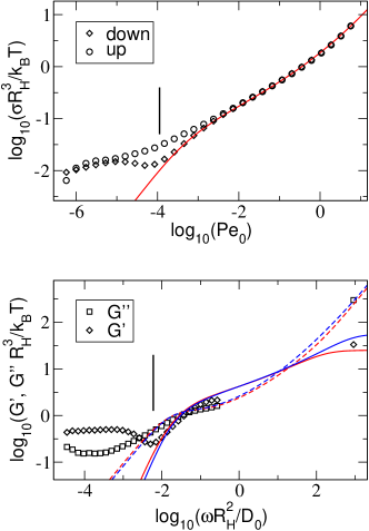
Figure 3: The reduced flow curves and the corresponding moduli for a fluid state at 13.01wt%, T$=20^{o}C$, and $\phi_{\rm eff}=0.540$. Flow curves measured proceeding from higher to lower shear rates (called ’down’ flow curves) and dynamic experiments were fitted where effects from crystallisation can be neglected; the lower limits of the unaffected-data regions are marked by vertical bars. The red lines show the fits with the schematic $F_{12}^{\left(\dot{\gamma}\right)}$-model while the blue lines show the results from microscopic MCT (solid $G^{\prime}$, broken $G^{\prime\prime}$), with parameters: $\varepsilon=-0.05$, $\frac{D_{S}}{D_{0}}=0.15$, and $\eta_{\infty}=0.3\,k_{B}T/(D_{0}R_{H})$; the moduli were scaled up by a factor $c_{y}=1.4$.

The small size polydispersity of the present particles enables the system to grow crystallites according to its equilibrium phase diagram. Fortunately, when recording flow curves, viz. stress as function of shear rate, data can be taken when decreasing the shear rate. We find that the resulting ’down’ flow curves correspond to amorphous states and reach the expected low-$\dot{\gamma}$ asymptotes ($\sigma=\eta_{0}\,\dot{\gamma}$, see Fig. 3), except for very low $\dot{\gamma}$, when an increase in stress indicates the formation of crystallites. ’Up’ flow curves, however, obtained when moving upwards in shear rate during the measurement of the stress are affected by crystallites formed after the initial shearing at 100 s^-1 during the timesweep and the first frequency sweep experiments. See the hysteresis between ’up’ and ’down’ flow curves in Figs. 3 and 4, where measurements for two fluid densities are reported. Above a critical shear rate $\dot{\gamma}_{\rm cr}\approx 4s^{-1}$ no hysteresis has been observed, which proved that all the crystallites have been molten. In the present work we focus on the ’down’ flow curves, and consider only data taken either for $\dot{\gamma}>\dot{\gamma}_{\rm cr}$, or (for $\dot{\gamma}<\dot{\gamma}_{\rm cr}$) before the time crystallisation sets in. This time was estimated from timesweep experiments as the time where crystallisation caused a 10$\%$ deviation of the complex modulus $G^{*}$. Thus, only the portions of the flow curves unaffected by crystallisation are taken into account; in Figs. 3 and 4 vertical bars denote the limits. We find that the effect of crystallisation on the flow curves is maximal around $\phi=0.55$ and becomes progressively smaller and shifts to lower shear rates for higher densities; see Figs. 3, 4 and 5. This agrees with the notion that the glass transition slows down the kinetics of crystallisation and causes the average size of crystallites to shrink.Meg:94 For the highest densities, which are in the glass without shear, the hysteresis at the lowest $\dot{\gamma}$ can be attributed to a non stationarity of the up curve; see Fig. 5. This effect has been confirmed by step flow experiments, but does not affect the back curves.

The linear response moduli similarly are affected by the presence of small crystallites at low frequencies. $G^{\prime}(\omega)$ and $G^{\prime\prime}(\omega)$ increase above the behavior expected for a solution ($G^{\prime}(\omega\to 0)\to\eta_{0}\,\omega$ and $G^{\prime\prime}(\omega\to 0)\to c\,\omega^{2}$) even at low density, and exhibit elastic contributions at low frequencies (apparent from $G^{\prime}(\omega)>G^{\prime\prime}(\omega)$); see Figs. 3 and 4. This effect follows the crystallisation of the system during the measurement after the shearing at $\dot{\gamma}=100$ $s^{-1}$. Only data will be considered in the following which were collected before the crystallisation time. For higher effective volume fraction other effects such as ageing and an ultra-slow process had to be taken into account and will be discussed more in detail in the next section.

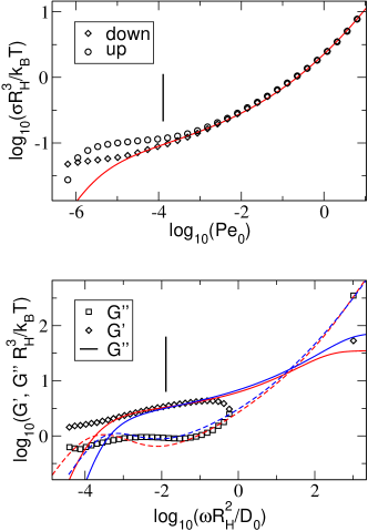
Figure 4: The reduced flow curves and the corresponding moduli (like in Fig. 3) for a fluid state at 13.01wt%, T$=18^{o}C$, and $\phi_{\rm eff}=0.567$. The vertical bars mark the minimal Peclet number or rescaled frequency for which the influence of crystallisation can be neglected. Microscopic parameters: $\varepsilon=-0.01$, $\frac{D_{S}}{D_{0}}=0.15$, and $\eta_{\infty}=0.3\,k_{B}T/(D_{0}R_{H})$; moduli scale factor $c_{y}=1.4$.

VI.2 Shapes of flow curves and moduli and their relations

The flow curves and moduli exhibit a qualitative change when increasing the effective packing fraction from around 50% to above 60%. For lower densities (see Fig. 3), the flow curves exhibit a Newtonian viscosity $\eta_{0}$ for small shear rates, followed by a sublinear increase of the stress with $\dot{\gamma}$; viz. a region of shear thinning behavior. For the same densities, the frequency dependent spectra exhibit a broad peak or shoulder, which corresponds to the final or $\alpha$-relaxation discussed in Sect. III. Its peak position (or alternatively the crossing of the moduli, $G^{\prime}=G^{\prime\prime}$) is roughly given by $\omega\tau=1$ (see Fig. 4). These properties characterize a viscoelastic fluid. For higher density, see Fig. 5, the stress in the flow curve remains above a finite yield value even for the smallest shear rates investigated. The corresponding storage modulus exhibits an elastic plateau at low frequencies. The loss modulus drops far below the elastic one. These observations characterize a soft solid. The loss modulus rises again at very low frequencies, which may indicate that the colloidal solid at this density is metastable and may have a finite lifetime (an ultra-slow process is discussed in Sect. VI.E).

Simple relations, like the ’Cox-Merz rule’, have sometimes been used in the past to compare the shapes of the flow curves $\sigma(\dot{\gamma})$ with the shapes of the dissipative modulus $G^{\prime\prime}(\omega)$. Both quantities can be interpreted in terms of a (generalized) viscosity, on the one hand as function of shear rate $\eta(\dot{\gamma})=\sigma(\dot{\gamma})/\dot{\gamma}$, and on the other hand as function of frequency $\eta(\omega)=G^{\prime\prime}(\omega)/\omega$. The Cox-Merz rule states that the functional forms of both viscosities coincide.

Figures 3 to 5 provide a sensitive test of relations in the shapes of $\sigma(\dot{\gamma})$ and $G^{\prime\prime}(\omega)$. Figure 4 shows most conclusively, that no simple relation between the far-from equilibrium stress as function of external rate of shearing exists with the equilibrium stress fluctuations at the corresponding frequency. While $\sigma(\dot{\gamma})$ increases monotonically, the dissipative modulus $G^{\prime\prime}(\omega)$ exhibits a minimum for fluid states close to the glass transition. It separates the low-lying final relaxation process in the fluid from the higher-frequency relaxation.

As shown in Fig. 2, the frequency dependence of $G^{\prime\prime}$ in the minimum region is given by the scaling function $\cal G$ of Sect. III, which describes the minimum as crossover between two power laws. The approximation for the modulus around the minimum

$$G^{\prime\prime}(\omega)\approx\frac{G_{\rm min}}{a+b}\;\left[\,b\,\left(\frac{\omega}{\omega_{\rm min}}\right)^{a}+a\,\left(\frac{\omega_{\rm min}}{\omega}\right)^{b}\,\right]$$ (29)

has been found in the quiescent fluid ($\varepsilon<0$, $\dot{\gamma}=0$), and works quantitatively if the relaxation time $\tau$ is large, viz.  time scale separation holds for small $|\varepsilon|$.Goe:91 The parameters in this approximation follow from Eqs. (17,18) which give $G_{\rm min}\propto\sqrt{-\varepsilon}$ and $\omega_{\rm min}\propto(-\varepsilon)^{1/2a}$. For packing fractions too far below the glass transition, the final relaxation process is not clearly separated from the high frequency relaxation. This holds in Fig. 3, where the final structural decay process only forms a shoulder. Closer to the transition, in Fig. 4, it is separated, but crystallisation effects prevent us from fitting Eq. (29) to the data.

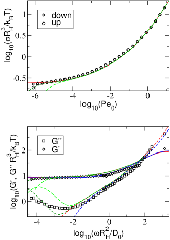
Figure 5: The reduced flow curves and the corresponding moduli for a glass state at 13.01wt%, T$=14^{o}C$, and $\phi_{\rm eff}=0.622$. See figure 3 for further explanations. Microscopic parameters: $\varepsilon=0.03$, $\frac{D_{S}}{D_{0}}=0.08$, and $\eta_{\infty}=0.3\,k_{B}T/(D_{0}R_{H})$; moduli scale factor $c_{y}=1.4$ (blue). Curves from the schematic F${}_{12}^{(\dot{\gamma})}$-model with an additional dissipative process included (Eq. 31) are shown as dashed lines; $\delta=10^{-7}\,\Gamma$ (long dashes, light green) and $\delta=10^{-8}\,\Gamma$ (short dashes, dark green). Here $\Gamma=88\,D_{0}/R_{H}^{2}$. The red curves give the schematic model calculations for identical parameters but without additional dissipative process (viz. $\delta=0$).

Asymptotic power-law expansions of $\sigma(\dot{\gamma})$ exist close to the glass transition, which were deduced from the stability analysis in Sect. III;Fuc:03 ; Hen:05 ; Haj:07 yet we refrain from entering their detailed discussion and describe the qualitative behavior in the following. For the same parameters in the fluid, where the minimum in $G^{\prime\prime}(\omega)$ appears, the flow curves follow a S-shape in a double logarithmic plot, crossing over from a linear behavior $\sigma=\eta_{0}\,\dot{\gamma}$ at low shear rates to a downward curved piece, followed by a point of inflection, and an upward curved piece, which finally goes over into a second linear behavior at very large shear rates, where $\sigma=\eta^{\dot{\gamma}}_{\infty}\,\dot{\gamma}$. This S-shape can be recognized in Figs. 3 and 4. Because of the finite slope of $\log_{10}{\sigma}$ versus $\log_{10}{\dot{\gamma}}$ at the point of inflection, one may speculate about an effective power-law $\log_{10}{\sigma}\approx c+c^{\prime}\log_{10}{\dot{\gamma}}$. In Fig. 3 this happens at Pe${}_{0}\approx 10^{-2}$. Yet, the power-law is only apparent because the point of inflection moves, the slope changes with distance to the glass transition, and the linear bit in the flow curve never extends over an appreciable window in $\dot{\gamma}$.Haj:07

Non-trivial power-laws in the flow curves exist close to the transition itself. At $\varepsilon=0$, a generalized Hershel-Bulkley law holds

$$\sigma(\dot{\gamma}\to 0)\to\sigma^{+}_{c}\left(1+|\frac{\dot{\gamma}}{\dot{\gamma}_{*}}|^{m}+c_{2}\,|\frac{\dot{\gamma}}{\dot{\gamma}_{*}}|^{2m}+c_{3}\,|\frac{\dot{\gamma}}{\dot{\gamma}_{*}}|^{3m}\right)$$ (30)

and describes the flow curves over an appreciable part of the range $\dot{\gamma}\leq\dot{\gamma}_{*}$, where structural relaxation dominates the stress;Hen:05 ; Haj:07 the exponent is $m=0.143$ in the F${}_{12}^{(\dot{\gamma})}$-model for this $\lambda$. It provides a semi-quantitative fit of the flow curves for more than a decade in $\dot{\gamma}$ close to the glass transition as shown in Fig. 6. There $|\varepsilon|$ is quite small at these effective packing fractions. A qualitative difference of the glass flow curves to the fluid S-shaped ones, is that the shape of $\sigma(\dot{\gamma})$ constantly has an upward curvature in double-logarithmic representation. The yield stress can be read off by extrapolating the flow curve to vanishing shear rate. In Fig. 5 this leads to a value $\sigma^{+}\approx 0.24\,k_{B}T/R_{H}^{3}$ at $\phi_{\rm eff}=0.622$, which is in agreement with previous measurements in this system over a much reduced window of shear rates.Fuc:05a ; Cra:06 While this agreement supports the prediction of an dynamic yield stress in the ITT approach, and demonstrates the usefulness of this concept, small deviations in the flow curve at low $\dot{\gamma}$ are present in Fig. 5. We postpone to Sect. VI.E the discussion of these deviations, which indicate the existence of an additional slow dissipative process in the glass. Its signature is seen most prominently in the loss modulus $G^{\prime\prime}(\omega)$ in Fig. 5.

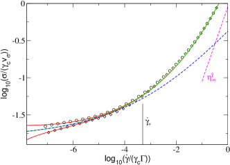
Figure 6: Flow curves for $\phi_{\rm eff}=0.580$ (diamonds) and $\phi_{\rm eff}=0.608$ (circles) rescaled with the parameters from the respective F${}_{12}^{(\dot{\gamma})}$-model fits; the corresponding fits are given as red solid lines, with separation parameter $\varepsilon=-2\,10^{-4}$ ($\phi_{\rm eff}=0.580$) and $\varepsilon=3\,10^{-4}$ ($\phi_{\rm eff}=0.608$). The blue dashed cuves gives the generalized Hershel-Bulkley law from Eq. (30), which holds at $\varepsilon=0$; for the F${}_{12}^{(\dot{\gamma})}$-model, its parameters are $\dot{\gamma}_{*}=5.06\,10^{-5}\Gamma=2.16\,10^{-5}/t_{0}$ (corresponding to a Peclet number Pe${}_{0}^{*}=4.25\,10^{-3}$ at $\phi_{\rm eff}=0.608$), $c_{2}\approx 0.936$, and $c_{3}\approx 0.632$. The green solid curve is the (critical) flow curve at $\varepsilon=0$ . The magenta dashed straight line labeled $\eta_{\infty}^{\dot{\gamma}}$ denotes the high-shear asymptote Eq. (27).

The storage modulus of the glass shows striking elastic behavior. $G^{\prime}(\omega)$ exhibits a near plateau over more than three decades in frequency, which allows to read off the elastic constant $G_{\infty}$ easily.

VI.3 Microscopic MCT results

Included in figures 3 to 5 are calculations using the microscopic MCT given by Eqs. (10) to (14) evaluated for hard spheres.numerics This is presently possible without shear only ($\dot{\gamma}=0$), because of the complications arising from anisotropy and time dependence in Eq. (12). The a priori unknown, adjustable parameter is the matching time scale $t_{0}$, which we adjusted by varying the short time diffusion coefficient appearing in the initial decay rate in Eq. (11). The computations were performed with $\Gamma_{{\bf q}}(t)\equiv\Gamma_{q}=D_{s}\,q^{2}/S_{q}$, and values for $D_{s}/D_{0}$ are reported in the captions of Figs. 3 to 5, and in table I. The viscous contribution to the stress is again mimicked by including $\eta_{\infty}$ like in Eq. (25).

Gratifyingly, the stress values computed from the microscopic approach are close to the measured ones; they are too small by 40% only, which may arise from the approximate structure factors entering the MCT calculation; the Percus-Yevick approximation was used here.russel In order to compare the shapes of the moduli the MCT calculations were scaled up by a factor $c_{y}=1.4$ in Figs. 3 to 5. Microscopic MCT also does not hit the correct value for the glass transition point.Goe:92 ; Goe:91 It finds $\phi^{\rm MCT}_{c}=0.516$, while our experiments give $\phi^{\rm exp}_{c}\approx 0.58$. Thus, when comparing, the relative separation from the respective transition point needs to be adjusted as, obviously, the spectra depend sensitively on the distance to the glass transition; the fitted values of the separation parameter $\varepsilon$ are included in Fig.8.

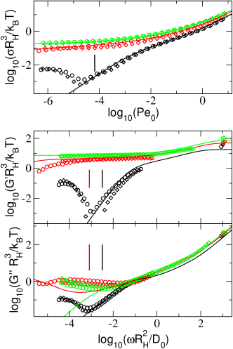
Figure 7: The plots demonstrate that the reduced flow curves and the reduced moduli are unique functions only depending on $\phi_{\rm eff}$. All flow curves are down curves. The fits using the schematic F${}_{12}^{(\dot{\gamma})}$-model were performed with the data points at 13.01wt% taken before the onset of crystallisation (data to the right of the vertical bars). Black diamonds: 12.10wt% and $\phi_{\rm eff}=0.527$. Black circles: 13.01wt% and $\phi_{\rm eff}=0.527$. Red diamonds: 12.10wt% and $\phi_{\rm eff}=0.578$. Red circles: 13.01wt% and $\phi_{\rm eff}=0.580$. Green diamonds: 13.01wt% and $\phi_{\rm eff}=0.608$. Green circles: 13.58wt% and $\phi_{\rm eff}=0.606$.

Considering the low frequency spectra in $G^{\prime}(\omega)$ and $G^{\prime\prime}(\omega)$, microscopic MCT and schematic model provide completely equivalent descriptions of the measured data. Differences in the fits in Figs. 3 to 5 for $\omega R_{H}^{2}/D_{0}\leq 1$ only remain because of slightly different choices of the fit parameters which were not tuned to be close. These differences serve to provide some estimate of uncertainties in the fitting procedures. Main conclusion of the comparisons is the agreement of the moduli from microscopic MCT, schematic ITT model, and from the measurements. This observation strongly supports the universality of the glass transition scenario which is a central line of reasoning in the ITT approach to the non-linear rheology.

At large $\dot{\gamma}$ and large $\omega$ hydrodynamic interactions become important. In the flow curves, $\eta_{\infty}^{\dot{\gamma}}$, and, in the loss modulus, $\eta_{\infty}^{\omega}$ become relevant parameters, and the structural relaxation captured in ITT and MCT is not sufficient alone to describe the rheology. Qualitative differences appear in the moduli, especially in $G^{\prime}(\omega)$, between the schematic model and the microscopic MCT. While the storage modulus of the F${}_{12}^{(\dot{\gamma})}$-model crosses over to a high-$\omega$ plateau already at rather low $\omega$, the microscopic modulus continues to increase for increasing frequency, especially at lower densities; see the region $\omega\,\raise 2.5pt\hbox{$>$}\hbox to0.0pt{\hss\lower 2.5pt\hbox{$\approx$}}\,10^{2}D_{0}/R_{H}^{2}$ in Figs. 3 to 4. The latter aspect is connected to the high-frequency divergence of the shear modulus of particles with hard sphere potential,Mas:95 as captured within the MCT approximation.Nae:98 ; numerics As carefully discussed by Lionberger and Russel, lubrication forces may suppress this divergence and its observation thus depends on the surface properties of the colloidal particles.Lio:94 Clearly, the region of (rather) universal properties arising from the non-equilibrium transition between shear-thinning fluid and yielding glass is left here, and particle specific effects become important.

VI.4 Parameters

In the microscopic ITT approach from Sect. II, the rheology is determined from the equilibrium structure factor $S_{q}$ alone. This holds at low enough frequencies and shear rates, and excludes the time scale parameter $t_{0}$ of Eq. (17), which needs to be found by matching to the short time dynamics. This prediction has as consequence that the flow curves and moduli should be a function only of the thermodynamic parameters characterizing the present system, viz. its structure factor.

Figure 7 supports this claim by proving that the rheological properties of the dispersion only depend on the effective packing fraction, if particle size is taken account of properly. Figure 7 collects flow curves and moduli measured for different concentrations of particles according to weight, and for different radii $R_{H}$ adjusted by temperature. Whenever the effective packing fraction, $\phi_{\rm eff}=(4\pi/3)nR_{H}^{3}$, is close, the rheological data overlap in the window of structural dynamics. Obviously, appropriate scales for frequency, shear rate and stress magnitudes need to be chosen to observe this. The dependence of the vertices on $S_{q}$ (Eqs. (10,II)) suggests that $k_{B}T$ sets the energy scale as long as repulsive interactions dominate the local packing. The length scale is set by the average particle separation, which can be taken to scale with $R_{H}$ in the present system. The time scale of the glassy rheology within ITT is given by $t_{0}$ from Eq. (17), which we take to scale with the measured dilute diffusion coefficient $D_{0}$. Thus the rescaling of the rheological data can be done with measured parameters alone. Figure 7 shows quite satisfactory scaling. Whether the particles are truely hard spheres is not of central importance to the data collapse in Fig. 7 as long as the static structure factor agrees for the $\phi_{\rm eff}$ used. Fits with the F${}_{12}^{(\dot{\gamma})}$-model to all data are possible, and are of comparable quality to the fits shown in Figs. 3 to 5.

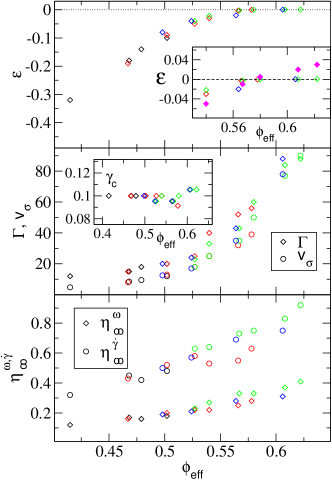
Figure 8: The fitted parameters of the F${}_{12}^{(\dot{\gamma})}$-model (open symbols). Black symbols: 10.75wt%, red symbols: 12.10wt%, green symbols: 13.01wt%, blue symbols: 13.58 wt%. $\varepsilon$ and $\gamma_{c}$ are dimensionless. Filled magenta symbols, included in the upper inset, give the $\varepsilon$ values fitted in the microscopic MCT calculations for 13.01wt%. The unit of $v_{\sigma}$ is $k_{B}T/R_{H}^{3}$ while $\Gamma$ is given in units of $D_{0}/R_{H}^{2}$. The high frequency and high shear viscosities $\eta_{\infty}^{\omega,\dot{\gamma}}$ are given in units of $k_{B}T/(D_{0}R_{H})$.

The fitted parameters used in the schematic F${}_{12}^{(\dot{\gamma})}$-model are summarized in Fig. 8. Parameters corresponding to identical concentrations by weight are marked by identical colours. Within the scatter of the data one may conclude that all fit parameters depend on the effective packing fraction only. This again supports the mentioned dependence of the glassy rheology on the equilibrium structure factor. The initial rate $\Gamma$, which sets $t_{0}$, appears a unique function of $\phi_{\rm eff}$, also; an observation which is not covered by the present ITT approach. It suggests that hydrodynamic interactions appear determined by $\phi_{\rm eff}$ in the present system also.

Importantly, all fit parameters exhibit smooth and monotonous drifts as function of the external thermodynamic control parameter, viz. $\phi_{\rm eff}$ here. Nevertheless, the moduli at low frequencies (e.g. $G^{\prime}(\omega)$ at $\omega R_{H}^{2}/D_{0}=0.01$), or the stresses at low shear rates (e.g. $\sigma(\dot{\gamma})$ at $\dot{\gamma}R_{H}^{2}/D_{0}=10^{-4}$) change by more than an order in magnitude in Figs. 3 to 5. Even larger changes may be obtained from taking experimental data not shown, whose fit parameters are included in Fig. 8. It is this sensitive dependence of the rheology on small changes of the external control parameters that ITT addresses.

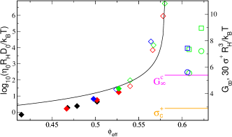
Figure 9: Newtonian viscosity $\eta_{0}$ (diamonds, left axis), elastic constant $G_{\infty}$ (squares), and yield stress $\sigma^{+}$ (circles; data rescaled by a factor 30; both $G_{\infty}$ and $\sigma^{+}$ right axis), as functions of the effective packing fraction $\phi_{\rm eff}$ as obtained from the fits performed with the F${}_{12}^{(\dot{\gamma})}$-model. Filled symbols indicate where direct measurements of $\eta_{0}$ were possible. Black symbols: 10.75wt%, red symbols: 12.10wt%, green symbols: 13.01wt%, blue symbols: 13.58 wt%. The line gives a power-law fit to the viscosity-data over the full range using the known $\gamma=2.34$ exponent from MCT, $\log_{10}{\eta_{0}}=A-\gamma\cdot\log_{10}\left(\phi_{\rm eff}^{c}-\phi_{\rm eff}\right)$; the critical packing fraction is found as $\phi_{\rm eff}^{c}=0.580$. Horizontal bars denote the critical elastic constant $G_{\infty}^{c}$, and the critical yield stress $\sigma^{+}_{c}$ as extrapolated from Fig. 6.

When comparing the parameters from the schematic model to the ones obtained from the microscopic MCT calculation of the moduli, one observes qualitative and semi-quantitative agreement; see the captions to Figs. 3 to 5, table I, and the upper inset of Fig. 8. For example, the increase of the prefactor $v_{\sigma}$ of stress fluctuations is captured in the microscopic vertex where $S_{q}$ enters (this follows because the rescaling factor $c_{y}$ is density independent). Also the hydrodynamic viscosity $\eta_{\infty}=\eta_{\infty}^{\omega}$ roughly agrees and may be taken $\phi_{\rm eff}$-independent in the fits with the microscopic moduli. The fitted values of $\eta_{\infty}$ are actually not too different from data obtained in Stokesian dynamics simulations of true hard spheres, supporting our simplified view on the particle interactions.Fos:00 On closer inspection, one may notice that the separation parameter of the microscopic hard sphere calculation obtains larger positive values than $\varepsilon$ fitted with the schematic model. Moreover, it follows an almost linear dependence on the effective packing fraction as asymptotically predicted by MCT, $\varepsilon\approx 0.65\,(\phi_{\rm eff}-\phi^{c}_{\rm eff})/\phi^{c}_{\rm eff}$ with glass transition density $\phi_{c}=0.587$ slightly higher than from the schematic model fits. The differing behavior of the separation parameter from the fits with the F${}_{12}^{(\dot{\gamma})}$-model in the glass is not understood presently. The microscopic calculation signals glassy arrest more clearly than the schematic model fit. The short time diffusion coefficient $D_{s}/D_{0}$ in the microscopic calculation decreases as expected from considerations of hydrodynamic interactions. Gratifyingly we find values in the range of the short-time self diffusion coefficient observed in Stokesian dynamics simulations for hard spheres.Ban:03 The initial rate $\Gamma$, however, of the schematic model increases with packing fraction. The ad hoc interpretatation of $\Gamma$ as microscopic initial decay rate evaluated for some typical wavevector $q_{*}$, viz. the ansatz $\Gamma=D_{s}q_{*}^{2}/S_{q_{*}}$, thus apparently does not hold.

$\phi_{\rm eff}$	$\varepsilon$	$D_{s}/D_{0}$	$\varepsilon^{\prime}$	$D^{\prime}_{s}/D_{0}$
0.527	- 0.08	0.15
0.540	- 0.05	0.15
0.567	- 0.01	0.15
0.580	0.005	0.13	- 0.01	0.15
0.608	0.02	0.11	- 0.003	0.15
0.622	0.03	0.08	- 0.003	0.15

Table 1: Parameters of the fits with the microscopic MCT to the linear-response moduli $G^{\prime}(\omega)$ and $G^{\prime\prime}(\omega)$. The first two columns of separation parameter $\varepsilon$ and short-time diffusion coefficient ratio $D_{s}/D_{0}$ correspond to the fits shown in Figs. 3 to 5 and Fig. 11 (solid lines), while the second columns of $\varepsilon^{\prime}$ and $D^{\prime}_{s}/D_{0}$ correspond to the dashed-lines in Fig. 11; when no value is given, the values from the first two columns apply. In all cases $c_{y}=1.4$ and $\eta_{\infty}=0.3\,k_{B}T/(D_{0}R_{H})$ are used.

While the model parameters adjusted in the fitting procedure only drift smoothly with density, the rheological properties of the dispersion change dramatically. Figure 9 shows the Newtonian viscosity as obtained from extrapolations of the fits in the F${}_{12}^{(\dot{\gamma})}$-model. It changes by 6 orders in magnitude. From the combination of $G^{\prime\prime}(\omega)$- and flow curve data we can follow this divergence over more than one decade in direct measurement. From the divergence of $\eta_{0}$ the estimate of the critical packing fraction can be obtained using the power-law Eq. (18), because the exponent $\gamma$ is known. We find $\phi_{\rm eff}^{c}=0.580$ in nice agreement with the value expected for colloidal hard spheres. On the glass side, the elastic constant and yield stress jump discontinuously into existence. Reasonable values are obtained from the F${}_{12}^{(\dot{\gamma})}$-model fits compared to data from comparable systems. The strong increase of the elastic quantities upon small increases of the density is apparent.

VI.5 Additional dissipative process in glass

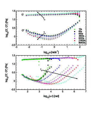
Figure 10: The storage $G^{\prime}(\omega)$ and loss $G^{\prime\prime}(\omega)$ moduli for different waiting times $t_{w}$. The data have been also plotted as function of $\omega t$ as suggested recently.Pur:06 See text for further explanation.

One of the major predictions of the ITT approach concerns the existence of glass states, which exhibit an elastic response for low frequencies under quiescent conditions, and which flow only because of shear and exhibit a dynamic yield stress under stationary shear. Figure 5 shows such glassy behavior, as is revealed by the analysis using the schematic and the microscopic model. Nevertheless, the loss modulus $G^{\prime\prime}(\omega)$ rises at low frequencies, clearly indicating the presence of a dissipative process. It is not accounted for by the present theory. Also, the storage modulus $G^{\prime}(\omega)$ shows some downward bend at the lowest frequencies.

These deviations can not be rationalized by ageing effects or non-linearities in the response; see Fig. 10. We checked the dependence on time since quench to this glass state and also the linear dependence of the stress on the shear amplitude. While we find ageing effects shortly after cessation of pre-shear,Pur:06 ; Sol:97 ; Sol:98 these saturate after one day, when the drifts of the spectra come to a stop. Ageing effects do not change the spectra qualitatively, as the dissipative process appears to possess a finite equilibrium relaxation time. As suggested recently for dense PNIPAM microgel dispersionsPur:06 the same data have been plotted as function of $\omega t$. Here, $t$ is the total waiting time and is defined as function of the waiting time $t_{w}$ before starting the measurement and the time $\delta(t(\omega_{n}))$ expired between $t_{w}$ and the acquisition of the data as $t=t(\omega_{n})=t_{w}+\delta(t(\omega_{n}))$. The curves collapse on a master curve in the low frequency range up to $\omega t\approx 3000$ as expected from ageing theory for waiting time $t_{w}<8200$ s. This prediction is no more respected for longer waiting times, where an additional relaxation process is identified. It cuts off the ageing behavior, when the age of the sample approaches the value of its relaxation time. This supports the introduction of an hopping phenomenon in our model, with a characteristic relaxation time of the order of $10^{4}$ s ($\approx R_{H}^{2}/\delta D_{0}=10^{8}R_{H}^{2}/\Gamma D_{0}=8.8\,10^{3}$ s see Fig.5).

Let us stress, moreover, that the state shown in Fig. 5 is not a fluid state within the present approach. The presence of an elastic window in $G^{\prime}(\omega)$, its increase as function of packing fraction, and the upward curvature of the flow curves rule out a negative separation parameter $\varepsilon<0$ of this state at $\phi_{\rm eff}=0.622$. Calculations within the microscopic MCT document this convincingly. Figure 11 compares the MCT calculations for hard spheres with moduli ranging from fluid to glassy states. By adjusting the effective packing fraction, MCT semi-quantitatively describes the dominating modulus, either loss or storage one, for all states (corresponding curves already shown in Figs 3 to 5). At high concentrations, it describes the storage modulus $G^{\prime}(\omega)$ on an error level of $1k_{B}T/R_{H}^{3}$, and misses the loss modulus $G^{\prime\prime}(\omega)$ by a similar absolute error. Yet, because the latter is itself of the order of $G^{\prime\prime}(\omega)\approx 1k_{B}T/R_{H}^{3}$ in the measurements, MCT fails to describe $G^{\prime\prime}(\omega)$ adequately. If, however, the effective packing fraction in the MCT calculations is adjusted to match the loss modulus $G^{\prime\prime}(\omega)$, then this fit fails completely to capture $G^{\prime}(\omega)$ at high densities; see the dashed lines in Fig. 11. Because the storage modulus, however, dominates the linear mechanical response of the glass, the second fit needs to be rejected. In conclusion, MCT correctly identifies the transition to a glass at high densities with dominating elastic response and yielding behavior under flow. It misses an additional dissipative process, which contributes on the 10% level to the shear moduli and stresses in the frequency and shear rate window explored in our experiments.

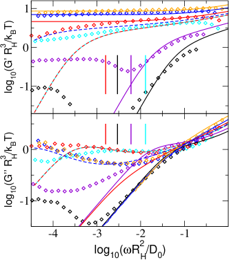
Figure 11: Fits with microscopic MCT to the linear-response moduli $G^{\prime}(\omega)$ (upper panel) and $G^{\prime\prime}(\omega)$ (lower panel) for the packing fractions $\phi_{\rm eff}=0.527$ (black diamonds and lines), $\phi_{\rm eff}=0.540$ (violet), $\phi_{\rm eff}=0.567$ (light blue), $\phi_{\rm eff}=0.580$ (red), $\phi_{\rm eff}=0.608$ (dark blue), and $\phi_{\rm eff}=0.622$ (orange). Continuous lines give the fits optimized for describing the storage modulus $G^{\prime}(\omega)$; these fits are also shown in Figs. 3 to 5, and the corresponding parameters are included in Fig. 8, and summarized in the left two columns in Table I. Broken lines for $\phi_{\rm eff}=0.580$ (red, overlapping with the solid light blue curve), and $\phi_{\rm eff}=0.608$ (dark blue; the same curve would fit $\phi_{\rm eff}=0.622$) show microscopic MCT calculations attempting to fit the minima in $G^{\prime\prime}(\omega)$ enforcing negative separation parameters $\varepsilon$ (parameters included in table I). These fluid like spectra can rationalize $G^{\prime\prime}(\omega)$, but fail qualitatively to describe $G^{\prime}(\omega)$. Vertical bars in corresponding colours denote the frequencies below which crystallisation affects the data at the different $\phi_{\rm eff}$.

The existence of an additional dissipative process contradicts the notion of ’ideal’ glass states as described by the present ITT or MCT aproach. Clearly, the system at $\phi_{\rm eff}=0.622$ becomes a fluid at even longer times, or lower shear rates and frequencies than observed in Fig. 5. This does not, however, contradict the observation that the structural relaxation as captured in the ITT equations has arrested. In an extension of the ITT approach, it is possible to account for the additional decay channel in a an extended schematic model; see the Appendix for details. Results from this extended F${}_{12}^{(\dot{\gamma})}$-model are included in Fig. 5 and demonstrate that none of the qualitative features discussed within ITT change at finite frequencies or shear rates. The additional process leads to fluid behavior at even lower $\omega$ or $\dot{\gamma}$, and needs to be taken into account only, if exceedingly small frequencies or shear rates are tested; its relaxation time at $\phi_{\rm eff}=0.622$ exceeds $10^{8}R_{H}^{2}/D_{0}=8.8.10^{3}$ s. It does not shift the location of the ’glass transition’ as defined within the idealized ITT (MCT) approach, because this is already determined by the shapes of the flow curves and spectra in the observed windows.

VII Conclusions

In the present study, we explored the connection between the physics of the glass transition and the rheology of dense colloidal dispersions, including in strong shear flow. Using model colloidal particles made of thermosensitive core-shell particles, we could investigate in detail the vicinity of the transition between a (shear-thinning) fluid and a (shear-molten) glass. The high sensitivity of the particle radius to temperature enabled us to closely vary the effective packing fraction around the critical value. We combined measurements of the equilibrium stress fluctuations, viz. linear storage and loss moduli, with measurements of flow curves, viz. nonlinear steady state shear stress versus shear rate, for identical external control parameters. In this way we could verify the consequences from the recent suggestion, that the glassy structural relaxation can be driven by shearing and in turn itself dominates the low shear or low frequency rheology.

In the employed theoretical approach, the equilibrium structure as captured in the equilibrium structure factor $S_{q}$ sufficed to describe all phenomena qualitatively. As only exception, we observed an ultra-slow decay of all glassy states that is yet not accounted for by theory. Microscopic calculations were possible for the linear response quantities using mode coupling theory applied to hard spheres. Schematic model calculations were possible within the integration through transients approach, and simultaneously captured the linear and nonlinear rheology using identical parameter sets. Semi-quantitative agreement between microscopic and schematic model calculations and with the measured data for varying effective packing fraction could be achieved adjusting a small number of fit parameters in smooth variations.

VIII Acknowledgements

We thank G. Petekidis and M. Cates for helpful discussions, and acknowledge financial support by the Deutsche Forschungsgemeinschaft in IRTG 667 ’Soft Condensed Matter Physics’. We acknowledge financial support by the DFG, SFB 481, Bayreuth, and by the Forschergruppe ’Nonlinear Dynamics of Complex Continua’, Bayreuth.

Appendix A Extended model including hopping

The ITT equations contain the feed back mechanism that the friction increases because of slow structural rearrangements. In the schematic F${}_{12}^{(\dot{\gamma})}$-model this is captured by the approximation for the generalized friction kernel $m(t)$ in Eq. (22). For $\dot{\gamma}=0$ it leads to non-ergodic glass states at large enough vertices $v_{1,2}$. A dissipative process explaining the fluidity of glassy states should renormalize the diffusion kernel $\Delta(t)$. Moreover, this mechanism should become more important the longer the relaxation time in $m(t)$. If, however, the additional dissipative process is too strong, all effects of the bare ITT approach are smeared out and the described phenomenology of the glass transition can not be observed.

Götze and Sjögren found when considering (possibly unrelated) dissipative processes in simple liquids that this can by achieved by splitting the diffusion kernel into two decay channels, one connected to the original $m(t)$, and the other one connected to the new dissipation mechanism. In order for the second decay channel to take over in glassy states, it suffices to model it by one additional parameter $\delta$ in a linear ansatz $\Delta^{\rm dissip}(t)=\delta\,m(t)$. This leads to the following replacement of Eq. (21) in the F${}_{12}^{(\dot{\gamma})}$-model

$$\partial_{t}\Phi(t)+\Gamma\left\{\!\Phi(t)+\!\!\int_{0}^{t}\!\!\!\!dt^{\prime}\,m(t\!-\!t^{\prime})\,\left[\partial_{t^{\prime}}\Phi(t^{\prime})\!+\delta\,\Phi(t^{\prime})\right]\!\right\}=0$$ (31)

The memory function $m(t)$ is still given by Eq. (22) because shearing decorrelates arbitrary fluctuations via shear-advection. All parameters of the model are kept as specified in Sect. IV, and solutions of this extended model with parameter $\delta$ given in the caption are included in Fig. 5. Importantly, the fluid like behavior in the rheology at exceedingly small $\dot{\gamma}$ and $\omega$ can now be captured without destroying the agreement with the original ITT at higher parameters. Apparently, a single parameter $\delta$ is not sufficient to model the non-exponential shape of the final relaxation process in the glass. Yet, further extensions of the model in order to describe this non-exponentiality go beyond our present aim.

References

References

- (1) R. G. Larson, The Structure and Rheology of Complex Fluids (Oxford University Press, New York, 1999).
- (2) W. B. Russel, D. A. Saville, and W. R. Schowalter, Colloidal Dispersions (Cambridge University Press, New York, 1989).
- (3) W. Götze and L. Sjögren, Rep. Prog. Phys. 55, 241 (1992).
- (4) P. N. Pusey and W. van Megen, Phys. Rev. Lett. 59, 2083 (1987).
- (5) W. Megen and P. N. Pusey, Phys. Rev. A, Phys. Rev. A 43, 5429 (1991).
- (6) W. van Megen and S. M. Underwood, Phys. Rev. Lett. 70, 2766 (1993).
- (7) W. van Megen and S. M. Underwood, Phys. Rev. E 49, 4206 (1994).
- (8) P. Hébraud, F. Lequeux, J. Munch and D. Pine, Phys. Rev. Lett. 78, 4657 (1997).
- (9) C. Beck, W. Härtl and R. Hempelmann, J. Chem. Phys. 111, 8209 (1999).
- (10) E. Bartsch, T. Eckert, C. Pies and H. Sillescu, J. Non-Cryst. Solids, 802, 307 (2002)
- (11) T. Eckert and E. Bartsch, Faraday Discuss. 123, 51 (2003).
- (12) E. R. Weeks, J. C. Crocker, A. C. Levitt, A. Schofield and D. A. Weitz, Science 287, 627 (2000).
- (13) T. G. Mason and D. A. Weitz, Phys. Rev. Lett. 75, 2770 (1995).
- (14) M. Zackrisson, A. Stradner, P. Schurtenberger and J. Bergenholtz, Phys. Rev. E 73, 011408 (2006).
- (15) H. Senff, W. Richtering, Ch. Norhausen, A. Weiss, M. Ballauff, Langmuir 15, 102 (1999).
- (16) H. Senff, W. Richtering, J. Chem. Phys. 111, 1705 (1999).
- (17) G. Petekidis, D. Vlassopoulos and P. Pusey, Faraday Discuss. 123, 287 (1999).
- (18) G. Petekidis,D Vlassopoulos, and P. N. Pusey, J. Phys.: Condens. Matter 16, S3955 (2004).
- (19) G. Petekidis, A. Moussaïd and P. Pusey, Phys. Rev. E 66, 051402 (2002).
- (20) K. N Pham, G Petekidis, D Vlassopoulos, S. U Egelhaaf, P. N Pusey, and W. C. K Poon, Europhys. Lett. 75, 624 (2006).
- (21) R. Besseling, Eric R. Weeks, A. B. Schofield and W. C. Poon, Phys. Rev. Lett. 99, 028301 (2007).
- (22) J. J. Crassous, M. Siebenbürger, M. Ballauff, M. Drechsler, O. Henrich and M. Fuchs, J. Chem. Phys. 125, 204906 (2006).
- (23) T. Phung, J. Brady and G. Bossis, J. Fluid Mech. 313, 181 (1996).
- (24) P. Strating, Phys. Rev. E 59, 2175 (1999).
- (25) B. Doliwa and A. Heuer, Phys. Rev. E 61, 6898 (2000).
- (26) E. H Purnomo, D. van den Ende, J Mellema and F Mugele, Europhys. Lett. 76, 74 (2006).
- (27) W. Götze, in Liquids, Freezing and Glass Transition, edited by J. P. Hansen, D. Levesque, and J. Zinn-Justin, Session LI (1989) of Les Houches Summer Schools of Theoretical Physics, (North-Holland, Amsterdam, 1991), 287.
- (28) W. Götze, J. Phys.: Condens. Matter 11, A1 (1999).
- (29) J. K. G. Dhont, An introduction to dynamics of colloids (Elsevier Science, Amsterdam, 1996).
- (30) H. M. Laun, R. Bung, S. Hess, W. Loose, O. Hess, K. Hahn, E. Hädicke, R. Hingmann, F. Schmidt and P. Lindner, J. Rheology 36, 743 (1992).
- (31) H. M. Wyss, K. Miyazaki, J. Mattsson, Z. Hu, D. R. Reichman and D. A. Weitz, Phys. Rev. Lett. 98, 238303 (2007)
- (32) J. F. Brady, J. Chem. Phys. 99, 567 (1993).
- (33) P. Sollich, F. Lequeux, P. Hébraud and M.E. Cates, Phys. Rev. Lett. 78, 2020 (1997)
- (34) P. Sollich, Phys. Rev. E 58, 738 (1998).
- (35) S. Fielding, P. Sollich, and M.E. Cates, J. Rheol. 44, 323 (2000)
- (36) L. Berthier, J.-L. Barrat and J. Kurchan, Phys. Rev. E 61, 5464 (2000).
- (37) L. Berthier and J.-L. Barrat, J. Chem. Phys. 116, 6228 (2002).
- (38) K. Miyazaki and D.R. Reichman, Phys.Rev.E. 66, 050501 (2002),
- (39) K. Miyazaki, D.R. Reichman and R. Yamamoto, Phys.Rev.E. 70, 011501 (2004).
- (40) V. Kobelev and K. S. Schweizer, Phys. Rev. E 71, 021401 (2005).
- (41) M. Fuchs and M. E. Cates, Phys. Rev. Lett. 89, 248304 (2002); M. Fuchs and M. E. Cates, in preparation (2007).
- (42) M. Fuchs and M. E. Cates, Faraday Disc. 123, 267 (2003).
- (43) M. Fuchs and M. E. Cates, J. Phys.: Condens. Matter 17, S1681 (2005)
- (44) F. Varnik and O. Henrich, Phys. Rev. B 73, 174209 (2006)
- (45) J. J. Crassous, A. Wittemann, M. Siebenbuerger, M. Drechsler and M. Ballauff, in preparation (2007)
- (46) Note that this discussion neglects the subtleties of the limit of infinite Peclet number,Brady1997 which corresponds to the limit of non-Brownian particles under shear,Dra:2002 and thus only provides insight into the limit of small to intermediate bare Peclet numbers.
- (47) J. F. Brady and J. F. Morris, J. Fluid Mech. 348, 103 (1997)
- (48) D. Drazer, J. Koplik, B. Khusid, and A. Acrivos, J. Fluid Mech. 460, 307 (2002)
- (49) Equation (II) presents a slightly simplified version of the general expression in Ref. Fuc:02 , restricting its use, so that only variables , like the shear stress , with and can be considered in the following.
- (50) G. Nägele and J. Bergenholtz, J. Chem. Phys. 108, 9893 (1998)
- (51) K. Miyazaki, H.M. Wyss, D. R. Reichman, D. A. Weitz Europhys. Lett. 75, 915 (2006)
- (52) J.M. Brader, Th. Voigtmann, M.E. Cates, and M. Fuchs, Phys. Rev. Lett. 98, 058301 (2007)
- (53) R. A. Lionberger and W. B. Russel, J. Rheol. 38, 1885 (1994).
- (54) Parameter is not yet well known as it could only be estimated in the isotropically sheared hard sphere model (ISHSM), which underestimates the effect of shear.Fuc:03 ; Bra:07
- (55) T. Franosch, W. Götze, M. R. Mayr, and A. P. Singh, J. Non-Cryst. Solids 235-237, 71 (1998).
- (56) W. Götze, Z. Phys. B 56, 139 (1984).
- (57) The schematic F-model of Refs. Fuc:05a ; Cra:06 differs by setting . This choice can be made by rescaling and if only a single experiment is considered.Haj:07
- (58) M. Fuchs and M. Ballauff, J. Chem. Phys. 122, 094707 (2005)
- (59) D. Hajnal and M. Fuchs, in preparation (2007)
- (60) N. Dingenouts, Ch. Norhausen and M. Ballauff, Macromolecules 31, 8912 (1998).
- (61) W. G. Hoover, S. G. Gray and K. W. Johnson, J. Chem. Phys. 55, 1128 (1971).
- (62) J. J. Crassous, R. Regisser, M. Ballauff and W. Willenbacher, J. Rheol. 49, 851 (2005).
- (63) I. Deike, M. Ballauff, N. Willenbacher, A. Weiss, J. Rheol. 45, 709 (2001).
- (64) G. Fritz, W. Pechhold, N. Willenbacher and J. W. Norman, J. Rheol. 47, 303 (2003).
- (65) For the numerical solution of the schematic model (Eqs. (21) to (25)) the algorithm of Ref. Fuc:91 was used, as has been done in previous studies. Fuc:05a ; Cra:06 The microscopic model (Eqs. (10) to (14)) was evaluated without shear for hard spheres with structure factor taken from the Percus-Yevick approximation;russel the wavevector integrals were discretized according to Ref. Fra:97 with only difference that wavevectors were chosen from up to with separation . Time was discretized with initial step-width , which was doubled each time after 400 steps. Note that the MCT shear modulus at short times depends sensitively on the large cut-off ;Nae:98 for hard spheres, gives the correct short time or high frequency divergence only for .
- (66) M. Fuchs, W. Götze, I. Hofacker, and A. Latz, J. Phys.: Condens. Matter 3, 5047-5071 (1991)
- (67) T. Franosch, M. Fuchs, W. Götze, M. R. Mayr, and A. P. Singh, Phys. Rev. E 55, 7153 (1997)
- (68) O. Henrich, F. Varnik and M. Fuchs, J. Phys.: Condens. Matter 17, S3625 (2005)
- (69) D. R. Foss and J. F. Brady, J. Fluid Mech. 407, 167 (2000).
- (70) A. J. Banchio and J. F. Brady, J. Chem. Phys. 118, 10323 (2003).