Far-from-equilibrium transport with constrained resources

Abstract

The totally asymmetric simple exclusion process (TASEP) is a well studied example of far-from-equilibrium dynamics. Here, we consider a TASEP with open boundaries but impose a global constraint on the total number of particles. In other words, the boundary reservoirs and the system must share a finite supply of particles. Using simulations and analytic arguments, we obtain the average particle density and current of the system, as a function of the boundary rates and the total number of particles. Our findings are relevant to biological transport problems if the availability of molecular motors becomes a rate-limiting factor.

Keywords: non-equilibrium statistical physics, totally asymmetric exclusion process, biological transport

1 Introduction

Over the last two decades, the study of driven diffusive systems [1, 2, 3, 4] has formed a significant branch in the general pursuit to understand non-equilibrium statistical mechanics. The underlying dynamics violates detailed balance, so that the long-time behavior is governed by a true non-equilibrium steady state (NESS). Highly unexpected and non-trivial properties are manifested, even in one-dimensional systems with purely local dynamics. A paradigmatic model in the last class is the totally asymmetric simple exclusion process (TASEP) [5, 6, 7, 8, 9, 4]. Characterized by open boundaries and particle transport, it displays the key physical signatures of a system driven far from equilibrium. In particular, its NESS develops a complex phase diagram controlled by the interactions of the system with its environment. While an understanding of these properties is of fundamental theoretical interest, the TASEP and its generalizations have also acquired fame as models for practical problems in traffic flow [10, 11] and biological transport [12, 13, 14, 15, 16, 17, 18, 19, 20, 21].

In this paper, we study a simple variant of the basic TASEP, by introducing a global constraint on the available number of particles. Deferring the motivations for such a model to the next paragraphs, let us briefly summarize the essentials. Each site of a one-dimensional lattice is either empty or occupied by a single particle. Following random sequential dynamics, the particles enter the lattice at one end (e.g., the “left” edge) with a given rate $\alpha$, hop to the right with rate $\gamma$ (scaled to unity), subject to an excluded volume constraint, and exit at the far end with a rate $\beta$. In the standard version of the model, both $\alpha$ and $\beta$ are constant rates, independent of the number of particles on the lattice. Thus, we may regard the lattice as being coupled to a reservoir – or a pool – with an arbitrarily large number of particles. Here, we consider a TASEP with a finite supply of particles and report our numerical and analytical findings. A fixed number of particles, $N_{tot}$, is shared between the lattice and the reservoir, in such a way that the entrance rate, $\alpha$, depends on the number in the pool: $N_{p}$. As a result, if more particles are found on the lattice, the number of available particles in the pool is lowered, leading to a corresponding decrease of $\alpha$. Since the number of particles on the TASEP lattice, $N$, feeds back into $\alpha$ through the constraint $N+N_{p}=$ constant $=N_{tot}$, we will refer to our model as “a constrained TASEP.” For simplicity, we assume the reservoir to be so large that particles exiting the lattice are unaffected by $N_{p}$, leaving $\beta$ unchanged. Our focus here is to explore the consequences of limited resources: How will the phase diagram and the properties of the phases be affected as the total number of available particles is reduced?

This behavior mimics the limited availability of resources required for a given physical or biological process. For example, in protein synthesis, ribosomes bind near the start sequence of a messenger RNA, in order to translate the genetic information encoded on the RNA into the associated protein. Ribosomes are large molecular motors which are assembled out of several basic units, and numerous ribosomes can be bound to the same, or other, mRNAs, so that multiple proteins are translated in parallel. When a protein is completed, the ribosome is disassembled and recycled into the cytoplasm. Under conditions of rapid cell growth, ribosomes or their constituents can find themselves in short supply, so that a self-limitation of translation, mimicked via a modification of $\alpha$, can occur. In a previous study [14], a different aspect of ribosome recyling was considered. This work focused on the enhancement of the ribosome concentration at the initiation site, as a result of diffusion of the ribosome subunits from the termination site (of the same mRNA). Due to the spatial proximity of initiation and termination sites, $\alpha$ is effectively increased. By contrast, our investigation of constrained resources leads to an effective reduction of $\alpha$.

In the context of traffic models, our problem corresponds to a generalization of the parking garage problem [22]. Here, one special site (the “parking garage”, or reservoir) is introduced into a TASEP on a ring (lattice with periodic boundary conditions) and, for this site only, the occupancy is unlimited. Particles (“cars”) jump into the garage with unit rate (corresponding to $\beta=1$), irrespective of its occupancy. Particles exit the garage with rate $\alpha$, provided the site following the garage is empty. As we will see presently, this is a special case of our more general model.

We begin with a description of our model and its observables of interest. Next, we outline results from simulations and compare them to a simple theory which builds on exact analytic results for the standard TASEP. We find excellent agreement for nearly all ($\alpha$,$\beta$) and conclude with some comments and open questions.

2 The model

The standard TASEP is defined on a one-dimensional lattice of length $L$, with sites labeled by $i$, $i=0,1,...,L-1$. Each site can be empty or occupied by a single particle, reflected through a set of occupation numbers $\{n_{i}\}$ which take the values $0$ or $1$. The boundaries of the lattice are open. Particles hop from a reservoir onto the lattice with a rate $\alpha$. Once on the lattice, particles will hop to the nearest-neighbor site on the right, provided it is empty. Once a particle reaches the end of the lattice, it hops back into the reservoir with rate $\beta$. The dynamics is random sequential, leading to fluctuations in the local occupations as well as in the total number of particles, defined via

$$N\equiv\sum_{i=0}^{L-1}n_{i}$$

The overall density is given by $\rho\equiv N/L$. Ensemble averages are denoted by $\left\langle...\right\rangle$.

Three distinct phases can be identified and are displayed in an $\left(\alpha,\beta\right)$ phase diagram (see Fig. 1): a low density (LD), a high density (HD), and a maximum current (MC) phase. The phases are distinguished, respectively, by their average densities: $\rho=\alpha\equiv\rho_{-}$, $\rho=1-\beta\equiv\rho_{+}$, and $\rho_{MC}=1/2$. The corresponding stationary currents are given by $J_{-}\equiv\alpha(1-\alpha)$, $J_{+}\equiv\beta(1-\beta)$, and $J_{MC}\equiv 1/4$. In all of these expressions, finite-size corrections have been neglected. Because of particle-hole symmetry, all aspects of the HD and LD phases are related. The phase boundaries between the HD and MC phases and between the LD and MC phases mark continuous transitions. The line separating the HD and LD phases, $\alpha=\beta<1/2$, is a coexistence line. Here, the system consists of a region with low density ($\rho_{-}$) followed by one with high density ($\rho_{+}$), connected by a microscopically sharp “shock.” This shock diffuses freely between the ends of the system, so that the average density profile is linear. Often this is referred to as the “shock phase” (SP).

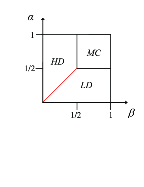
Figure 1: Phase diagram of the standard TASEP.

The system of interest here differs from the standard TASEP in one important way: The number of particles in the reservoir, $N_{p}$, is finite, and we choose the on-rate $\alpha$ to depend on $N_{p}$ as follows. So as to distinguish this varying rate from the $\alpha$ of the ordinary TASEP, we denote the former as the effective on-rate $\alpha_{eff}$ and write

$$\alpha_{eff}\left(N_{p}\right)=\alpha f(N_{p})\,\,,$$

where $f(x)$ is a function that satisfies three conditions: (i) $f(0)=0$, (ii) $f(\infty)=1$, and (iii) $f(x)$ is monotonically increasing. The first of these conditions is self-evident; the second simply connects our model to the standard one with unlimited resources; the last is just common sense. In this notation, the “parking garage” problem [22] is characterized by $f(N_{p})=\theta(N_{p})$ where $\theta$ is the Heaviside step function. Here, we wish to model, say, a cell with finite number of ribosomes, so that it is natural to assume that a smaller number of particles in the pool results in a lower on-rate, etc., and that $f$ would be a smoother function. Specifically, for the simulations shown below we choose

$$f(N_{p})=\tanh\left(N_{p}/N^{\ast}\right)$$ (1)

where $N^{\ast}$ provides the scale for crossover to saturation. The detailed choice of $N^{\ast}$ is unimportant, but it is convenient to make it extensive in $L$. For easier comparison, we choose $N^{\ast}$ to be the average (stationary) density of the unconstrained TASEP defined by the parameters $\left(\alpha,\beta\right)$: For example, if $\alpha>1/2,\beta<1/2$ (HD phase, ordinarily), we set $N^{\ast}$ to $L\rho_{+}=L(1-\beta)$. For the SP, we arbitrarily choose $N^{\ast}=L/2$. To summarize, the control parameters of our model are the same as the ordinary TASEP ($\alpha,\beta;L$) plus the total number of particles, $N_{tot}$ (i.e., $N+N_{p}$).

To characterize our system in steady state, we measure the average density $\rho\equiv\langle N\rangle/L$, the average (local) density profile $\rho_{i}\equiv\langle n_{i}\rangle/L$, and the average current $J$. For the last quantity, we record the total number of particles entering and leaving the chain over the run (thereby improving statistics) and divide the average of these by the length of the run.

In our Monte Carlo simulations, we pick randomly from the $N$ particles on the lattice and one additional virtual particle. If a lattice particle is selected, we attempt to update its position as in ordinary TASEP; if the virtual particle is selected, we attempt to place a new particle on the first site of the chain. $N+1$ attempts constitute one Monte Carlo Step (MCS). Initially, the chain is empty, i.e., $N=0$, $N_{p}=N_{tot}$. Typically, the first $10^{6}$ ($10^{7}$ for SP) MCS are discarded, to ensure that the system has reached steady state, before data are taken. Then, configurational observables are recorded every $100$ MCS and averaged until the run terminates. The typical length of each run is $10^{7}$ ($10^{8}$ for SP) MCS. Longer runs are required to obtain low noise data for density profiles and currents. Statistical errors were estimated through visual inspections of time series and through multiple runs, to ensure the reproducibility of the data. We simulated system sizes in the range of $L=250$ to $L=8000$, with most data taken for $L=1000$. To obtain the phase diagram, we simulated more than a dozen $\left(\alpha,\beta\right)$ pairs. Here, we report results for four points: $\left(0.25,0.75\right)$, $\left(0.75,0.25\right)$, $\left(0.75,0.75\right)$, and $\left(0.25,0.25\right)$. Since these correspond, respectively, to LD, HD, MC, and SP in a standard TASEP, we will use these letters to refer to the four cases studied.

3 Results from simulations

In this section, we summarize our simulation results. Since only the on-rate depends on the feedback, the behavior of our system is no longer governed by particle-hole symmetry. As a result, the simplest case is the first in the above, i.e., “LD”. Both $\rho$ and $J$ increase with $N_{tot}$ in an expected fashion. The next case, MC, is already slightly more interesting: Both $\rho$ and $J$ increase until the effective on-rate reaches 1/2, after which both become constant. The end result is a pronounced kink in $\rho$. The HD case provides an even more interesting scenario: The system properties range through three regions as $N_{tot}$ is increased. Finally, the SP provides the most unexpected behavior. In the next section, we turn to a simple theoretical description of our findings.

The LD case. Here, we set $\alpha<1/2$, $\beta>\alpha$, and vary the total number of particles, $N_{tot}$, in the system. With $f$ given by Eqn (1), our simulation results for $L=1000$ and $\left(\alpha,\beta\right)=\left(0.25,0.75\right)$ are shown in Fig. 2. As expected, we see that, for large $N_{tot}$, the system density $\rho=\left\langle N\right\rangle/L$ approaches the value for the standard TASEP for $N_{tot}\gg N^{\ast}$ (here, $0.75L$), namely, $\rho=\alpha$ (which is $0.25$ in our case). More interestingly, for $N_{tot}\lesssim N^{\ast}$, we find a reduced density, $\rho<\alpha$, a signal that the system is responding to the limited availability of particles from the reservoir. In the limit $N_{tot}\rightarrow 0$, $\rho$ naturally vanishes, with a predictable slope (see below). The current $J$ in this “phase” also decreases monotonically with decreasing $N_{tot}$, from its asymptotic limit $\beta(1-\beta)$ (given by $0.1875$).

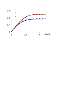
Figure 2: Average density $\rho$ and current $J$ vs $N_{tot}/L$ for an LD case ($L=1000$, $\alpha=0.25$, and $\beta=0.75$). Open circles and diamonds are from the analysis in Section 4.

The MC case. This domain of the phase diagram is characterized by $\alpha>1/2$ and $\beta>1/2$ in the standard TASEP. Fig. 3 shows the averages $\rho$ and $J$, as $N_{tot}$ varies, for $(\alpha,\beta)=(0.75,0.75)$. The former displays a single kink, just below $N_{tot}/L\simeq 1.0$, accompanied by a rather smooth crossover in the current. As we will see below, this kink is associated with a crossover from an MC-like behavior to an LD-like behavior, as $N_{tot}$ drops below the value required to sustain a density $\rho_{MC}=1/2$ on the chain.

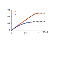
Figure 3: Average density $\rho$ and current $J$ vs $N_{tot}/L$ for an MC case ($L=1000$, $\alpha=0.75$, and $\beta=0.75$). Open circles and diamonds are from the analysis in Section 4.

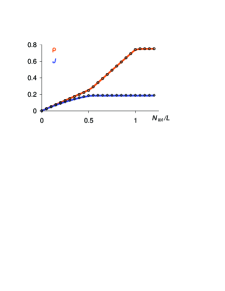
Figure 4: Average density $\rho$ and current $J$ vs $N_{tot}/L$ for an HD case ($L=1000$, $\alpha=0.75$, and $\beta=0.25$). Open circles and diamonds are from the analysis in Section 4. The predictions from domain wall theory (not shown) are similiar.

The HD case. Here, we set $\beta<1/2$ and $\alpha>\beta$. Fig. 4 shows our results for $(\alpha,\beta)=\left(0.75,0.25\right)$. As expected, for sufficiently high $N_{tot}$, the system settles into the density and current associated with the HD phase of the standard TASEP: $\rho=0.749\simeq\rho_{+}$, and $J=0.184\simeq\beta\left(1-\beta\right)$. As $N_{tot}$ is reduced, to the extent that the chain is prevented from sustaining a density of $\rho_{+}$, the naive expectation is that a crossover to an LD-like behavior appears. Remarkably, however, Fig. 4 shows not just two, but three distinct regimes, separated by two pronounced “kinks” at $N_{tot}\,/L\simeq 0.5$ and $1.0$. As Fig. 5 illustrates, these kinks become sharper with increasing $L$. Looking for potentially critical behavior, we measured the variance of $\langle N\rangle$ near the kinks and compared it to its values deep within each regime. To our surprise, at least for the $L=1000$ system, the variance was not noticeably larger at the kinks than at other locations. Simulations at larger values of $L$ would be required to settle this issue with more certainty.

The current $J$ is also displayed in Fig. 4. For low values of $N_{tot}/L$, $J$ increases in an expected way. Around $N_{tot}=0.5L$, it shows a distinct kink and then becomes essentially constant, with a value of $0.184$. This is close to $0.1875$, the value of $J$ for infinite $L$. Since the current appears to have already reached the “asymptotic” value here, it is not too surprising that there is no sign of a “second kink” (near $N_{tot}=L$, where $\rho$ has another one). Below, we offer a theoretical description for these findings.

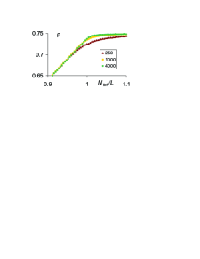
Figure 5: Finite-size effects on the kink in $\rho$, near $N_{tot}/L=1.0$, for the HD case in Fig. 4:$\;L=250$, $1000$, and $4000$.

The SP case. Defined in the standard TASEP by $\alpha=\beta<1/2$, this line of first-order phase transitions separates the HD and LD phases. Though the average density is 1/2, its fluctuations are large. In particular, since a shock (which separates a region with density $\rho_{+}$ from one with $\rho_{-}$) diffuses freely between the ends of the system, the probability $P(\rho)$ of finding the system with a density $\rho$ approaches a flat distribution: $P(\rho)=\theta(\rho-\rho_{-})\theta(\rho_{+}-\rho)/\left(\rho_{+}-\rho_{-}\right)$, in the limit $L\rightarrow\infty$. Of course, finite-size effects will smooth out the steps at $\rho_{+}$ and $\rho_{-}$. Imposing finite resources, we may expect that $\rho$ increases simply with $N_{tot}$ as in the LD case, perhaps rising more slowly to the asymptotic value of 1/2. Instead, its properties are much more subtle. As illustrated in Fig. 6 (for $\alpha=\beta=0.25$), $\rho$ increases with $N_{tot}/L$, slows, speeds up, and slows down again. The behavior in the low $N_{tot}$ regime is intuitively understandable, since there are too few particles to sustain any phase other than LD. The large $N_{tot}$ regime is also expected. In the crossover regime ($L\lesssim N_{tot}\lesssim 3L$), an intriguing “shoulder” develops. Though this behavior is accounted for by the domain wall theory [23, 24] (see below), we have found no simple and intuitive way to understand it. Perhaps the presence of large fluctuations, as the system gets closer to the SP, smooths out the two kinks observed in the HD case. To gain more insight, we investigated $P(\rho)$. Fig. 7 shows particle density histograms (gathered from 50K data points and plotted with arbitrary normalization here), for several choices of $N_{tot}/L$. For low $N_{tot}/L$ (e.g., 0.5 in the figure), our system is dominated by the lack of resources, so that this distribution is essentially Gaussian, quite similar to those measured deep within the LD phase. As $N_{tot}/L$ increases, the system enters the crossover regime and $P(\rho)$ becomes quite asymmetric, as a detailed fitting of the $N_{tot}/L=1.0$ case shows. At the other extreme, this distribution is indeed relatively flat. However, the true asymptotic regime is reached only for very large $N_{tot}/L$. Thus, the slope for even the $N_{tot}/L=3.0$ case (cf. Fig. 7) is discernably non-zero. Throughout the intermediate regime, the structure of $P$ is more interesting. Each histogram has the cross-section of a “lean-to” (a shack with a slanted roof). A more detailed inspection shows that the “roof” is predominantly a (slowly) decaying exponential . This picture is consistent with the one from domain wall theory [23, 24], as will be discussed below. It is this slow crossover - from well-defined Gaussians to a completely flat distribution - which accounts for the interesting structure in the rise of $\rho$ with $N_{tot}/L$.

Finally, the behavior of the current is also sensitive to the slow crossover, although it displays no interesting structures like those in $\rho$. Comparing Fig. 6 with the earlier ones, we see that it saturates at values of $N_{tot}/L$ which are 2 to 3 times higher than in the other cases.

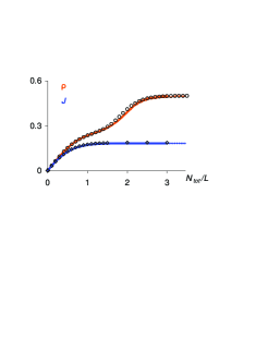
Figure 6: Average density $\rho$ and current $J$ vs $N_{tot}/L$ for an SP case ($L=1000$, $\alpha=0.25$, and $\beta=0.25$). Open circles are from the domain wall theory in Section 4. Open diamonds are the current computed from Eqn (2).

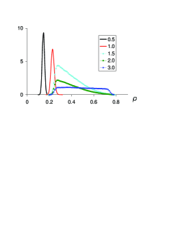
Figure 7: Histograms of the density $\rho$ for $L=1000$, $\alpha=0.25$, and $\beta=0.25$. (For ease of comparisons, the histograms with solid lines only are scaled down by 2.) Legend shows various values of $N_{tot}/L$.

4 Analytic predictions

In the steady state of a standard TASEP, the overall density of particles is controlled only by the entrance and exit rates. It is natural to expect that these relations would also hold in our case, except that the stationary density needs to be determined from the (variable) entrance rate in a self-consistent way. In the following, we pursue this approach and compare it to the simulation results reported in the preceding section.

The LD case. Again, we begin with a choice of $(\alpha,\beta)$ such that the system is in an LD phase, with $\rho<1/2$. Invoking the exact expression for the density of the standard TASEP, namely, $\rho=\alpha$, we write the density of particles in the resource-limited case as $\rho=\alpha_{eff}=\alpha f(N_{p})$. With $N_{p}=N_{tot}-L\rho$, this becomes an implicit equation for $\rho$:

$$\rho=\alpha f(N_{tot}-L\rho)$$ (2)

which can be solved for given $\alpha$ and $N_{tot}$. Specifically, since $0\leq f(N_{tot}-L\rho)\leq 1$, the solution will lie between $0$ and $\alpha$. The upper bound will be reached if $N_{tot}/L\rightarrow\infty$ so that the right hand side of Eqn (2) remains essentially constant as a function of $\rho$. For any finite value of $N_{tot}/L$, the right hand side is a monotonically decreasing function of $\rho$ so that (i) Eqn (2) always has a solution, and (ii) the solution decreases monotonically with $N_{tot}/L$. The resulting density, and the associated current, $J=\alpha_{eff}\left(1-\alpha_{eff}\right)$, are shown as open circles and diamonds, respectively, in Fig. 2, for the choice of $f$ given in Eqn (1). We see, in particular, that for small values of $N_{tot}/L$, we may use $\tanh x\simeq x$ whence $\rho\simeq N_{tot}/(2L)$. Clearly, the agreement with the simulation data is impressive.

The MC case. After these considerations, the analysis of the MC phase is quite straightforward. For large $N_{tot}$, the density saturates at $\rho=1/2$, with $J=1/4$. For small $N_{tot}$, the system is LD-like and follows Eqn (2). The transition occurs when $\alpha_{eff}$ is forced to drop below $1/2$, i.e., at the intersection of Eqn (2) and $\rho=1/2$. Here, $N_{tot}$ assumes the critical value of $N_{tot,c}$, given by

$$N_{tot,c}=L\rho+f^{-1}\left(\frac{1}{2\alpha}\right)\,.$$ (3)

The current follows the behavior of the density.

The HD case. Next, we turn to the high-density phase, with $\beta<1/2$ and $\alpha>\beta$. If the number of available particles is very large, we may again invoke the exact relation for the density of the standard TASEP, namely

$$\rho=\rho_{+}=1-\beta\,.$$ (4)

This reflects the constant density observed in the simulations. Clearly, this cannot be sustained as the number of available particles is reduced, since the effective $\alpha$ of the system is also reduced. A transition should be expected when it reaches $\beta$. $=\alpha_{eff}=\alpha f(N_{p})$. Translating $\beta$ $=\alpha_{eff}$ into an equation for the system density $\rho$, we arrive at

$$\beta=\alpha_{eff}=\alpha f(N_{tot}-L\rho)\,\,.$$ (5)

Solving for $\rho$, and setting it to the one from Eqn (4), we find the critical value of the total particle number for this transition: $N_{tot.2}=L\left(1-\beta\right)+f^{-1}\left(\beta/\alpha\right)$. (The subscript, $2$, helps to distinguish it from the lower transition point.) For the specific $f$ used in simulations, this results in

$$N_{tot.2}=L\left(1-\beta\right)\left[1+\tanh^{-1}\frac{\beta}{\alpha}\right].$$ (6)

As we see, $N_{tot.2}/L=0.75\left[1+\tanh^{-1}\left(1/3\right)\right]\simeq 1.01$ is in excellent agreement with the “second kink” shown in Fig. 4.

At the opposite extreme, the resources are very low, so that $\alpha_{eff}$ is significantly less than $\beta$, and the system is pushed into LD-like behavior. For such low $N_{tot}$, the density follows Eqn (2). In this regime, $f$ is well approximated by a linear function, so that $\rho\simeq\alpha(N_{tot}-L\rho)/N^{\ast}=\alpha(N_{tot}/L-\rho)/\left(1-\beta\right)$, i.e.,

$$\rho\simeq\frac{\alpha}{1-\beta+\alpha}N_{tot}/L\,\,.$$

Of course, Eqn (2) is also not “sustainable,” in the sense that $\rho\rightarrow\alpha$ for large $N_{tot}$ instead of the correct limit: $\rho\rightarrow 1-\beta$. The critical value of $N_{tot}$ again occurs when $\alpha_{eff}$ reaches $\beta$, i.e., when the density given by Eqn (2) reaches $\beta$. The result is

$$N_{tot.1}=L\beta+L\left(1-\beta\right)\tanh^{-1}\left(\frac{\beta}{\alpha}\right).$$ (7)

Again, for the case shown in Fig. 4, there is excellent agreement between the data and this prediction: $N_{tot.1}/L\simeq 0.51$.

Between $N_{tot.1}$ and $N_{tot.2}$, Eqn (5) provides a linear dependence of $\rho$ on $N_{tot}/L$

$$\rho=N_{tot}/L-f^{-1}\left(\beta/\alpha\right)/L\,\,,$$ (8)

with unit slope. Again, with no fitting parameters, this theoretical prediction agrees remarkably well with the observations. In this regime, the reservoir occupation (and so $\alpha_{eff}$) remains constant, while the change in $N_{tot}$ is balanced by the change in total lattice population: $L\rho$. Since $\alpha_{eff}=\beta$ (on the average), the current remains at the constant value $J=\beta\left(1-\beta\right)$ throughout.

While this “three-piece” approach is both intuitively appealing and surprisingly successful in reproducing simulation data, it begs the question: Is there a unified theory that is just as successful with predictions? The answer is affirmative, namely, the domain wall theory [23, 24]. Since this theory is absolutely indispensable for providing good predictions for the next case, we will discuss its details in the next subsection.

The SP case. Here, Monte Carlo simulations presented us with unexpected phenomena: the “shoulder” in Fig. 6 for $\rho$. The simple approach taken above succeeds only in predicting the behavior for the extreme values of $N_{tot}/L$. Dominated by the limited resources, the solution of $\rho=\alpha_{eff}$ fits the data very well for $N_{tot}/L\lesssim 1$. At the other extreme ($N_{tot}/L\gg 1$), the system is necessarily in the SP, where $\rho=1/2$ on the average. In the crossover regime, the understanding of the structure in $\rho\left(N_{tot}/L\right)$ requires a more sophisticated theory [23, 24]. Based on a biased random walk of the shock (i.e., domain wall), Santen and Appert [24] derived the average occupation for a finite TASEP:

$$\left\langle N\right\rangle=\rho_{-}L+\delta\left\{\frac{r}{1-r}-\left(L+1\right)\frac{r^{L+1}}{1-r^{L+1}}\right\}$$ (9)

where $\delta=\rho_{+}-\rho_{-}=\left(1-\beta\right)-\alpha$, and

$$r=\frac{\alpha\left(1-\alpha\right)}{\beta\left(1-\beta\right)}$$ (10)

is the ratio of the diffusion constants to the right/left. To apply to our SP case, we simply set $\alpha$ to be $\alpha_{eff}=\beta f(N_{tot}-L\rho)$ in this equation. That sets up a relationship between $\rho$ and $N_{tot}/L$ which can be computed numerically. The agreement between this theory and data is quite respectable (Fig. 6), though not as spectacular as in the other cases. Not surprisingly, most of the disagreement occurs in the crossover region. We believe that the main difficulty lies with the large fluctuations of the domain wall, feeding back in non-trivial ways to the on-rate.

For another perspective on the successes and limitations of this theory, we can compare $P(\rho)$ above with the predicted $P_{i}$, the probability of finding the domain wall to be at site $i$. The latter is, for the steady state, a pure exponential [23, 24]: $P_{i}\propto\exp\left(i/\xi\right)$. Since our focus here is the dependence on $\rho$, $P_{i}$ can be translated into $P(\rho)$, via the relation $\rho=\rho_{+}\left(1-i/L\right)+\rho_{-}\left(i/L\right)$. We find that the predicted $P(\rho)$ is proportional to $\exp\left(-\rho/\sigma\right)$, and nonzero only in the interval $[\rho_{-},\rho_{+}]$. Our simulations show several non-trivial deviations from this theoretical prediction, however. (i) The slopes in the exponent are systematically steeper than predicted. (ii) Quadratic terms in $\ln P(\rho)$ are far from negligible. (iii) The tails of $P(\rho)$ extend substantially outside the range $\left[\rho_{-},\rho_{+}\right]$. In other words, there is room for improvements to the domain wall theory.

Another intriguing phenomenon, not shown here explicitly, is the complex dependence of this crossover on $L$. In particular, both simulations and theory show that the “shoulder” completely disappears for small $L$. For example, in an $L=100$ run, $\rho\left(N_{tot}/L\right)$ rises linearly for $N_{tot}/L\lesssim 1.5$ and simply “slows down” into the asymptotic value of $1/2$ for $N_{tot}/L\gtrsim 2.5$. For large $L$, in contrast, there exists a subtle competition between the factors $\left(L+1\right)$ and $r^{L+1}$ in Eqn (9). The result is that the crossover region gets longer with larger $L$, producing challenges at the simulations front as well. Of course, these difficulties are hardly surprising, since the complexities here are undoubtedly due to large fluctuations associated with the infrared scales. Further studies into this issue, especially more detailed investigations of the lean-to’s in $P(\rho)$, should provide insight for a better understanding of such fluctuations.

To conclude this section, we briefly note that we also simulated an alternate form of the on-rate, namely, $f(N_{p})=1/\left[1+\left(N^{\ast}/N_{p}\right)^{2}\right]$. We will not present any details here, but the agreement of simulation data and analytic results for the three regimes (HD, LD, and MC) is equally convincing. However, the details of the crossover regime in SP are likely to be quite sensitive to functional form of $f$.

5 Conclusions

In this paper, we studied a TASEP with open boundary conditions. In contrast to the standard model, where the particles are supplied by an infinite reservoir, the total number of available particles in our model, $N_{tot}$, is fixed. Mimicking limited resources, the available particles are shared between the reservoir and the system itself: If more particles bind to the chain, the reservoir is depleted, and vice versa. We account for this situation through an effective on-rate, $\alpha_{eff}$, which depends on $N_{p}$, the number of particles in the pool, and hence, on $N$, the number on the chain. Specifically, we mainly used Eqn (1), $\alpha_{eff}=\alpha\tanh\left(N_{p}/N^{\ast}\right)$, here. As the number of available particles is reduced from infinity, the system crosses over from the asymptotic behavior of the standard TASEP to different behaviors dominated by limited resources.

If the corresponding standard model (i.e., $N_{tot}\rightarrow\infty$ limit) lies in the LD phase, there are no surprises in either $\rho$, the average particle density on the chain, or $J$, the average current: Both are proportional to $N_{tot}$ for $N_{tot}\ll L$, crossing gently over to the asymptotic values much like the $\tanh$ function. For the MC phase, there is already a sublety: both $\rho$ and $J$ increase monotonically and then, at a characteristic $\alpha_{eff}$ ($=1/2$) become constant. $\rho$ displays a notable kink there. For the other two cases (HD and SP), $\rho$ exhibits an additional, intermediate regime (though the behavior of $J$ shows little hint of this regime). In the HD case, $\rho$ is linear in $N_{tot}/L$ with unit slope; only the intercept depends on $\alpha/\beta$. Here, $N_{p}$ remains constant, as any increase in $N_{tot}/L$ is “absorbed” by the chain (through a shift in the domain wall). This behavior may be regarded in the same light as an equilibrium system with phase co-existence. Considering, e.g., the pressure vs. volume isotherm for a liquid-gas system below criticality, the pressure remains constant over some range, as any increase in volume is absorbed by a shift in the liquid-to-gas ratio.

The most interesting and challenging case is the SP. In the intermediate regime, a “shoulder” appears in $\rho\left(N_{tot}/L\right)$. In addition, this structure displays a non-trivial dependence on $L$. Although the predictions of domain wall theory agree reasonably well with MC data, there are small ($\lesssim 6\%$) systematic discrepancies. We also investigated histograms of particle densities, which cross over from sharply peaked Gaussians for $N_{tot}\ll L$ to a flat distribution (between $\rho_{-}=\beta$ and $\rho_{+}=1-\beta$) for $N_{tot}\gg L$. In the intermediate regime, this distribution displays a much richer behavior than a truncated exponential – the result of domain wall theory.

Several questions remain open for further study. First, are the transitions between the three regimes in HD associated with true thermodynamic singularities? We find that the changes in slope accompanying these “crossovers” become sharper with increasing chain length $L$. While this speaks for a true transition, the absence of large fluctuations is somewhat surprising. Clearly, a more careful analysis is required to explore these questions more fully.

Second, though domain wall theory is reasonably successful for $\rho\left(N_{tot}/L\right)$ in the SP case, we would like to find improvements of this approach, so as to account for the crossover regime better. Arriving at a good understanding of $P(\rho)$ and the large fluctuations would be desirable. Progress along these lines may also help us to develop an intuitive picture for the complex $L$ dependence.

Finally, we are mindful of one of the motivations of this study, namely, finite resources in biological systems, e.g., ribosomes (and aa-tRNA’s) for modeling protein synthesis in a cell [12, 13, 15, 16, 17, 18]. For that application, the above TASEP needs to be generalized, to include exclusion at a distance (particles covering more than one site) and inhomogeneous hopping rates. How these systems are affected by finite resources will pose many interesting new challenges, especially on the theoretical frontier.

Acknowledgements. We thank Travis Merritt for preliminary simulation results and Meesoon Ha and Marcel den Nijs for helpful discussions. This work was supported in part by the National Science Foundation through DMR-0414122 and DMR-0705152.

References

- [1] Katz S, Lebowitz J L and Spohn H 1983 Phys. Rev. B 28 1655, and 1984 J. Stat. Phys. 34 497
- [2] Schmittmann B and Zia R K P, 1995 Phase Transition and Critical Phenomena, Vol. 15, edited by Domb C and Lebowitz J L (London, Academic Press)
- [3] Privman V, 1997 Nonequilibrium Statistical Mechanics in One Dimension (Cambridge, Cambridge University Press)
- [4] Schütz G M, 2000 Phase Transition and Critical Phenomena, Vol. 19, edited by Domb C and Lebowitz J L (San Diego: Academic Press)
- [5] Krug J, 1991 Phys. Rev. Lett. 67 1882
- [6] Derrida B, Domany E, and Mukamel D, 1992 J. Stat. Phys. 69 667
- [7] Derrida B, Evans M R, Hakim V, and Pasquier V, 1993 J. Phys. A: Math. Gen. 26 1493
- [8] Schütz G M and Domany E, 1993 J. Stat. Phys. 72 277
- [9] Derrida B, 1998 Phys. Rep. 301 65
- [10] Chowdhury D, Santen L, and Schadschneider A, 2000 Phys. Rep. 329 199
- [11] Popkov V, Santen L, Schadschneider A, and Schütz G M, 2001 J. Phys. A: Math. Gen. 34 L45
- [12] MacDonald C, Gibbs J, and Pipkin A, 1968 Biopolymers 6 1
- [13] MacDonald C and Gibbs J, 1969 Biopolymers 7 707
- [14] Chou T, 2003 Biophys. J. 85 755
- [15] Shaw L B, Zia R K P, and Lee K H, 2003 Phys. Rev. E 68 021910
- [16] Chou T and Lakatos G, 2004 Phys. Rev. Lett. 93 198101
- [17] Dong J J, Schmittmann B, and Zia R K P, 2007 J. Stat. Phys. 128 21
- [18] Dong J J, Schmittmann B, and Zia R K P, 2007 Phys. Rev. E 76 051113
- [19] Howard J, 2001 Mechanics of Motor Proteins and the Cytoskeleton (Sunderland: Sinauer Assoc.)
- [20] Kolomeisky A B and Fisher M E, 2007 Ann. Re. Phys. Chem. 58 675
- [21] Basu A and Chowdhury D, 2007 Phys. Rev. E 75 021902
- [22] Ha M and den Nijs M, 2002 Phys. Rev. E 66 036118
- [23] Kolomeisky A B, Schütz G M, Kolomeisky E B, and Straley J P, 1998 J. Phys. A: Math. Gen. 31 6911; Belitzky V and Schütz G M, 2002 El. J. Prob. 7 Paper no. 11
- [24] Santen L and Appert C, 2002 J. Stat. Phys. 106 187