Correlated Link Shadow Fading in Multi-hop Wireless Networks
Abstract
Accurate representation of the physical layer is required for analysis and simulation of multi-hop networking in sensor, ad hoc, and mesh networks. This paper investigates, models, and analyzes the correlations that exist in shadow fading between links in multi-hop networks. Radio links that are geographically proximate often experience similar environmental shadowing effects and thus have correlated fading. We describe a measurement procedure and campaign to measure a large number of multi-hop networks in an ensemble of environments. The measurements show statistically significant correlations among shadowing experienced on different links in the network, with correlation coefficients up to 0.33. We propose a statistical model for the shadowing correlation between link pairs which shows strong agreement with the measurements, and we compare the new model with an existing shadowing correlation model of Gudmundson (1991). Finally, we analyze multi-hop paths in three and four node networks using both correlated and independent shadowing models and show that independent shadowing models can underestimate the probability of route failure by a factor of two or greater.
Index Terms:
Wireless sensor, ad hoc, mesh networks, shadowing, correlation, statistical channel model, wireless communication, measurement, performanceI Introduction
Both simulation and analysis are critical to the development of multi-hop networks, including mesh, ad hoc, and sensor networks. However, current physical layer models do not accurately represent radio channels in multi-hop wireless networks [1], and as a result, there is a significant disconnect between simulation and real world deployment. There is significant interest in improving statistical models beyond the current state-of-the-art in order to decrease the difference between simulation and analysis results and experimental deployment results.
This paper presents a statistical joint path loss model between a set of static nodes. Joint path losses and transmit powers determine the connectivity, reliability in interference, and energy consumption during power control, of network communications. Channel models used in multi-hop networks have considered path losses to be independent, yet they are correlated through shadowing effects. We demonstrate these correlations via measurements and present a correlated shadowing loss model, which is then shown to have a dramatic effect on network connectivity.
We do not address other random processes like transmit power variation, manufacturing variations among nodes, position of nodes in random deployments, mobility of nodes, or interference models. However, the developed model informs future development of path loss models for mobile networks, and may be used to analyze the effects of other variation and interference models.
I-A Single-Link Path Loss Model
Radio propagation measurement and modeling for a single radio link has been reported extensively over the past century [2, 3, 4, 5]. In general, when there is no site-specific knowledge of the environment, the ensemble mean received power, (dBm), at a distance from the transmitter, is [3, 4],
| (1) |
where is the transmitted power in dBm, is the path loss exponent, and is the loss experienced at a short reference distance from the transmitter antenna. This model incorporates the free space path loss model when , and extends to practical (obstructed) multipath environments when .
On a particular link, received power will vary from the ensemble mean because of fading. The measured received power for the link between transmitter and receiver is,
| (2) |
where is the distance between nodes and , and is the fading loss. In general, shadow fading, small-scale or frequency-selective fading, and antenna and device losses all contribute to . Wideband receivers reduce the effects of small-scale or frequency-selective fading issues, and antenna and device-caused variations are generally small compared to shadowing variations. Shadow fading, also called medium-scale fading [3], describes the loss suffered as the signal passes through or diffracts around major obstructions in its path from the transmitter to the receiver. These obstructions include walls and furniture indoors, and buildings, terrain, and trees outdoors.
We hypothesize that shadowing losses are correlated across different links which are geographically proximate. Since shadowing is central to the analysis in this paper, we separate total fading loss into two contributions,
| (3) |
where represents the shadowing loss, and represents all other (non-shadowing) losses.
I-B Application in Multi-hop Networking Research
In the multi-hop networking simulation and analysis literature, two models are used:
-
1.
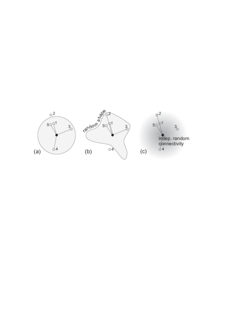
The circular coverage model: for all links, and thus the coverage area is a perfect circle, as shown in Figure 1(a).
-
2.
The i.i.d. log-normal shadowing model: For all links , random variables are independent and identically distributed Gaussian with zero mean and variance , as shown in Figure 1(c).
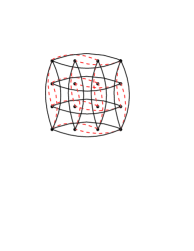
We argue that both models are at opposite extremes, and both problematic. Note that ‘realistic coverage’ is commonly depicted pictorially as a coverage area with random range as a function of angle [6, 7], as in Figure 1(b), and neither fading model produces such a random shape. It is easy to recognize that the deterministic, circular coverage areas are unrealistic for wireless communications links. However, circular coverage has been a common assumption in ad hoc and sensor network research and has been used to generate foundational research results. Kotz, Newport, and Elliot [8] examined the set of papers in the MobiCom proceedings from 1995 through 2002, and found that out of 36 papers which required radio models, only four did not use a circular coverage model.
In comparison, the i.i.d. shadowing model is non-deterministic, and eliminates the concept of coverage area. Since the model has no spatial memory, even two nearly overlapping links would be represented as statistically independent. For example node 2 in Figure 1(c) may be connected while node 1 is not.
Recent research, including Hekmat and Van Mieghem [7] and Bettstetter and Hartmann [6], has studied connectivity in ad hoc networks using the i.i.d. log-normal shadowing model. Their analyses indicate that for a constant level of connectivity, node deployment density can be reduced when the variance of the shadowing is increased. This increase in connectivity is largely a result of the model’s independence assumption. Since losses in links in the same direction from a transmitter are independent, if one link is disconnected because of high loss, another node in the same direction is likely to be connected.
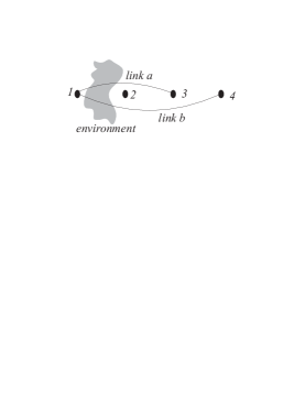
In reality, if an obstacle in one direction from a transmitter strongly attenuates its signal, any receiver behind the obstacle is likely to experience high fading loss. For example, if the environment in Figure 2 causes severe shadowing, it is likely to cause additional path loss on both links and . In contrast, the i.i.d. log-normal shadowing model assumes that the shadowing across links and will be independent and thus exaggerate the connectivity. We quantify this argument in Section VII.
I-C Correlation Limits Link Diversity
Diversity methods are common means to achieve reliability in unreliable channels. Multi-hop networking serves as a network-layer diversity scheme by allowing two nodes to be connected by any one of several multi-hop paths. All diversity schemes are limited by channel correlations. Correlations have been studied and shown to limit diversity gains in time, space, frequency and multipath diversity schemes [9, 3, 4, 10].
Yet little research has addressed channel correlations on links in sensor, mesh, and ad hoc networks. This paper presents an initial investigation into quantitatively assessing the correlation in the shadow fading experienced on the different links of a multi-hop network. This investigation is experimental, using full link measurements of an ensemble of deployed networks to estimate and test for statistical correlations. We propose a joint path loss model which accurately represents observed correlations in link shadowing. Further, we quantify the effect that such correlation has on source to destination path statistics. We show that for a simple three node network that the probability of path failure is double what would be predicted by the i.i.d. log-normal shadowing model.
II Related Work
Shadow fading correlations have been measured and shown to be significant in other wireless networks. For example: (1.) in digital broadcasting, links between multiple broadcast antennas to a single receiver have correlated shadowing which affects the coverage area and interference characteristics [11]; (2.) in indoor WLANs correlated shadowing is significant (as high as 0.95) strongly impacts system performance [12]; and (3.) in cellular radio correlation on links between a mobile station and multiple base stations significantly affects mobile hand-off probabilities and co-channel interference ratios [13, 14, 15].
In cellular radio, the model of Gudmundson [16] is used to predict shadowing correlation for the link between a mobile station (MS) to a base station over time as the MS moves. In Section VI, we address the difficulty in applying this model to multi-hop networks. We quantitatively compare it with the proposed model when the Gudmundson model may be applied. Wang, Tameh, and Nix [17] extended Gudmundson’s model to the case of simultaneous mobility of both ends of the link, for use in MANETs, and relate a sun-of-sinusoids method to generate realizations of the shadowing process in simulation. Both works use “correlated shadowing” to refer to the correlation of path loss in a single link over time, while the present work studies the correlation of many disparate links at a single time.
The closest study to the present work used RSS measurements in a single network to quantify correlations between two links with a common node [18]. Those results could not be complete because a single measured network cannot provide information about an ensemble of network deployments. The present study uses multiple measured networks to examine many pairs of links with the identical geometry, both with and without a common node.
III Measurement Setup
In this section we present our method for measuring the path-loss of each pair-wise link in a multi-hop network, using a specialized sensor network. This system is referred to as the network channel measurement system (NCMS). The NMCS allows us to quickly measure the received power (dBm) of every link in a deployed network, to measure across a range of frequencies, and to record the data on a laptop for later analysis.
III-A Equipment
The nodes used in the measurement campaign are “mica2” motes manufactured by Crossbow. A mica2 mote operates in the 902 - 928 MHz band using a Chipcon CC1000 FSK transceiver. The transmit power is user programable and can be varied based on the network topology and environmental density. The mica2 measures and reports RSS values for each received signal [19].
III-A1 Battery Variations
Transmit power is proportional to the battery voltage squared. Since measurement and data collection of one deployed network take on the order of minutes, battery voltage can be considered constant during each experiment. Each device measures and reports its own battery voltage, and we monitor to ensure that battery voltages are largely the same across devices throughout the experiment.
III-B Protocol
III-B1 Software
A NesC/TinyOS embedded program is written to operate the following protocol:
Frequency Hopping
From the 902-928 MHz band, 14 center frequencies are chosen. The nodes are programmed such that each node hops across all the 14 frequencies in each cycle. The time duration between frequency hops is three seconds.
Synchronization
Synchronization is required so that frequency-hopping sensors are all transmitting and receiving on the same frequency at the same time. One of the frequencies in the frequency band is considered as a synchronization frequency and is repeated three times each cycle so that neighbors can synchronize with each other more quickly. The dwell time on each frequency includes a period in which all sensors transmit a packet and receive packets from other sensors, and a period for switching frequency.
Pairwise measurements
Each node measures path loss on all links with all other nodes at each frequency. A TDMA-based MAC scheme is used in which each node broadcasts its pairwise measurements during an assigned slot, to avoid interference. The data sent by a node in its packet transmission includes the RSS values recorded during the previous period, a unique sequence number, its transmit power, and its battery voltage.
III-B2 Receiver Base
The receiver base is a mica2 node connected to a laptop, loaded with a special receiver program which synchronizes to the frequency hopping schedule of the nodes and communicates all the received packets serially to the laptop for storage and later analysis.
IV Experiment
This section describes the use of the NCMS described in Section III to measure a network deployed in an ensemble of 15 different environments. These measurements will enable the statistical analysis and model development in subsequent sections.
IV-A Motivation
Ideally, statistical characterization of the radio channel for multi-hop networks would proceed as follows: deploy K networks, each with N nodes positioned with the identical geometry in the same type of environment, but each network in a different place. For example, one might deploy the NCMS in a grid, in K different office buildings.
In reality, its not economical to carry out the measurement campaign in different office buildings, mainly because it is difficult to obtain access to carry out measurement in many different office areas, and it is difficult to position sensors in exactly the same geometry without moving obstructions to make space for each node. If the environment must be altered to measure it, we might as well randomly alter the entire environment.
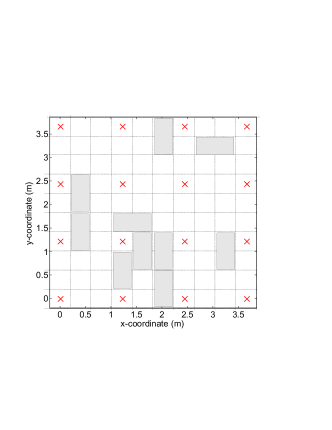
In fact, in this campaign, we occupy a single environment and randomly vary the object locations in that environment. We start by deploying nodes in an empty classroom in the Merrill Engineering Building at the University of Utah. A 4x4 square grid of mica2 nodes is set up with 4 ft (1.22 m) separation between neighboring sensors. Within this deployment area, different arrangements of obstructions are randomly generated.
IV-A1 Random Environment Generation
For reasons of portability, the obstructions used in this campaign were cardboard boxes of size 61 cm x 41 cm x 61 cm (24 in x 20 in x 25 in). In order to make the boxes significant RF scatterers, we wrap the cardboard boxes with aluminium foil. Foil-wrapped cardboard boxes represent metal obstacles which might be present in office environments.
We generate (in Matlab) random positions for 10 boxes to be placed in the area of the deployment. The Matlab script is written to ensure that boxes do not lay on top of any of the 16 sensors (which are placed on the floor). Beyond that restriction, the rectangular boxes may be positioned anywhere in the environment and may be positioned with either N-S or E-W orientation i.e., with their longer sides parallel or perpendicular to the X-axis as shown in Fig. 3.
IV-B Experiment Procedure
After random placement of the 10 obstructions, the campaign proceeds by powering on the 16 nodes and receiving and recording the measured path loss data in a file on a laptop. Each node runs the algorithm described in Section III. After 10 minutes of run-time, the nodes are turned off. The process continues with the next measured network by randomly changing the obstruction locations and repeating the experiment. Fifteen network realizations are measured in this manner.
V Statistical Analysis
This section presents the statistical analysis of the data collected by campaign described in Section IV. We first estimate the path loss model parameters of (1) and (2). Next, we analyze the shadowing loss correlations which exist on different pairs of links.
V-A Analysis of Received Power
We denote the number of the deployment experiment as , where is the number of deployments (here, ). We denote the set of frequencies measured as . The received signal power between node and node for experiment at center frequency is denoted and can be written using (2) and (3) as
| (4) |
where is the non-shadow fading and is the shadow fading on link during experiment . Shadow fading is considered to be constant across the frequency band, as discussed in Section I. We denote the frequency average received power as ,
From (4), we can write as,
| (5) |
In other words, (5) can be written as,
| (6) |
where . Because is an average of measurements at many different frequencies, we argue that it may be well-represented as Gaussian (in dB), regardless of the underlying frequency-selective fading mechanism (e.g., Rayleigh or Rician). Since is also log-normal [20], we expect the sum to also be Gaussian (in dB).
A linear regression of the frequency averaged received signal powers versus known distances is used to estimate the constants and (6) for each experiment . In our experiments, we have used m. Since all nodes are set to the same transmit power and have approximately equal battery voltages, and since we estimate in addition to , we are not required to know the exact transmit power at the current battery voltage of the nodes in the network during experiment . The linear regression also determines the variance of .
V-B Analysis of Link Correlations
In this subsection, we describe the computation of the correlation in fading between pairs of links. This requires computing correlation in the sample values of for different pairs of links as described in Section V-A.
V-B1 Similar Geometry Links
We use the term “link geometry” to describe for two links, link and link , the relative coordinates of the end points of the two links. In a grid network, there can be many pairs of links with the same link geometry (within a rotation). As one example, the link pair of link and link shown in Fig. 2, is repeated 16 times in the network as shown in Fig. 4.
Let denote the number of times a particular link geometry is repeated in the network. We denote the link pair as the two links and , where . Then and , where , represent the total fading on the repeated link pair for experiment number . Then vectors and are defined as
| (7) |
We then define vectors and as
| (8) |
Vectors and are both x1 sized vectors. Together they contain all measured total fading values for pairs of links which share a particular link geometry. The correlation coefficient of total fading on link and link , , can be computed by taking vectors and as sample values of total fading for link and link respectively.
We have computed the correlation coefficient for total fading on link and link for a variety of link geometries. Table I shows the results for various link pair geometries. We also run a hypothesis test to determine if the measured correlation is statistically significant. This test compares hypotheses,
We report using the method described in [21, pp. 427-431], in Table I. The proposed correlated link shadowing model and the Gudmundson model, also mentioned in Table I, will be discussed in Section VI.
| Geometry | Correlation | Geometry | Correlation | ||||||
|---|---|---|---|---|---|---|---|---|---|
| Meas- | Prop. | Gud. | Meas- | Prop. | Gud. | ||||
| ured | Model | model | ured | Model | model | ||||
| 1 | 0.33*** | 0.21 | 0.13 | 15 | -0.04 | 0.05 | 0.04 | ||
| 2 | 0.21*** | 0.17 | 0.04 | 16 | 0.12*** | 0.10 | 0.08 | ||
| 3 | 0.23*** | 0.24 | 0.13 | 17 | 0.08* | 0.07 | 0.08 | ||
| 4 | 0.05 | 0.03 | 0.04 | 18 | 0.12*** | 0.11 | 0.04 | ||
| 5 | 0.17*** | 0.19 | n/a | 19 | 0.03 | 0.10 | 0.08 | ||
| 6 | -0.05 | 0.00 | n/a | 20 | 0.21*** | 0.13 | 0.13 | ||
| 7 | -0.01 | 0.00 | n/a | 21 | -0.02 | 0.08 | 0.04 | ||
| 8 | -0.10** | 0.00 | n/a | 22 | 0.23*** | 0.16 | 0.13 | ||
| 9 | -0.03 | 0.05 | 0.04 | 23 | 0.00 | 0.05 | 0.04 | ||
| 10 | 0.18*** | 0.21 | 0.08 | 24 | 0.06 | 0.16 | 0.08 | ||
| 11 | 0.04* | 0.08 | 0.13 | 25 | 0.08** | 0.13 | n/a | ||
| 12 | 0.14*** | 0.08 | 0.13 | 26 | 0.12 | 0.16 | n/a | ||
| 13 | 0.17*** | 0.08 | 0.13 | 27 | 0.08 | 0.00 | n/a | ||
| 14 | 0.05 | 0.06 | 0.08 | 28 | 0.03 | 0.02 | 0.02 | ||
| p- value or | ||
| *** | ** | * |
V-C Discussion
The results show that, for many link pair geometries, it is extremely unlikely that the fading losses measured on the pair of links are independent. For 15 of the 28 studied link geometries, there is statistically significant non-zero correlation. Those 15 links are consistently those geometries in which the two links are proximate, i.e., their lines from transmitter to receiver partially overlap, or nearly overlap. The likelihood that the measured correlation coefficient was measured by chance in the case when is extremely small, i.e., less than 0.5%, for 11 of the 15 link geometries which showed correlation.
Also note that the correlation coefficients are relatively large in magnitude. The highest is 0.33, six link geometries have , and eleven link geometries have . Fading loss on one link is obviously not purely determined by the losses experienced on its geographically proximate links; however, the correlation coefficient indicates that knowing the losses on the proximate links can give quite a bit of information about the loss on that one link.
VI Joint Path Loss Model
In this section we present a model to describe the experimentally observed characteristic of correlated link shadowing. We start with the assumption that shadowing loss experienced on the links in a network is a result of an underlying spatial loss field , such that shadowing on a link is increased when its path crosses areas of high loss . We show how this assumption results in agreement with existing path loss models when considering a single link. We then show how it accurately represents correlated shadowing losses when jointly considering links in a multi-hop network.
VI-A Shadow Fading Model
In particular, we assume that the underlying spatial loss field is an isotropic wide-sense stationary Gaussian random field with zero mean and exponentially-decaying spatial correlation. The covariance between at positions and as
| (9) |
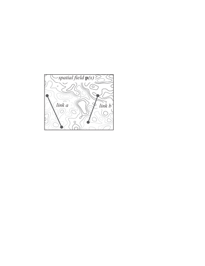
where is the Euclidian distance between and , is a space constant and is the standard deviation of the shadow fading. The contour plot of a realization of such a random process is shown in Figure 5.
Many mathematically valid spatial covariance functions are possible [22]. We justify the use the covariance function in (9) because of its basis in a Poisson spatial random process. Poisson processes are commonly used for modeling the distribution of randomly arranged points in space, and we suppose that attenuating obstructions might be modeled in such a fashion as well. Without detailing a specific model for the spatial extent or value of attenuation of each obstruction, we note that many Poisson processes (or derivatives of Poisson processes) have covariance functions with an exponential decay as a function of distance, as (9).
We propose to model the shadowing on all links as functions of the spatial loss field. We propose to model the shadowing on link , , as
| (10) |
Single-Link Properties
This model agrees with two important empirically-observed link shadowing properties:
- Prop-I
-
Prop-II
Shadow fading losses are Gaussian.
The model in (10) can be seen to have Prop-II, since is a scaled integral of a Gaussian random process.
Joint Link Properties
Next, consider two links and , as shown in Fig. 5 with shadowing and , respectively. Consider the covariance of and ,
| (14) |
where is the line between points and . Since , the correlation coefficient between and , , is
| (15) | ||||
The solution to (15) is tedious to analytically derive. We use numerical integration to compute the value of , and Matlab calculation code is available on the authors’ web site [23].
VI-B Total Fading Model
Since shadowing loss is only one part of the total fading loss , we must also consider the model for non-shadowing losses . It is worthwhile to note that shadow fading and non-shadow fading are caused by different physical phenomenon, and thus and can be considered as independent. The variance is thus
| (16) |
Non-shadow fading is predominantly composed of frequency-selective or small-scale fading, which can be well-approximated to have zero correlation over distances greater than a few wavelengths. Since multi-hop networks typically have sensors spaced more than a few wavelengths apart, are considered independent in this paper.
Thus the correlation coefficient between the total fading on links and , and , is
| (17) |
Equation (17) indicates a linear relationship between the correlation coefficient of total fading and correlation coefficient of shadow fading. The correlation coefficient, , is the measured computed in Table I. The total fading variance was determined by the regression analysis in Section V-A.
VI-C Estimation of model parameters from measurements
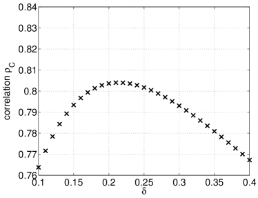
Both the space constant and the variance of shadowing must be determined experimentally from the data set. Specifically, we find the pair which best explains the correlations which exist in the link measurements. In other words, the goal is to find the value of that results in highest agreement between measured and model-based correlation values.
To accomplish this model fitting, we compute the model correlation, , for a range of using (15), for each of the 28 link geometries considered in Table I. At a particular value of , we compare the model correlation with the measured correlation using linear regression. This linear regression returns a correlation coefficient, , which quantifies how well the model (using ) agrees with the measurements. The highest value of uses , the optimum which matches the model to the measurements. Fig. 6 plots the correlation for . We can observe that the curve attains the maximum at . The value of is then determined from using (17), and we see that .
In summary, we have determined the two parameters of the correlation model, using the measurement data set.
VI-D Comparison with Gudmundson Model
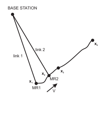
In this section, we compare the proposed model of shadow fading correlation with an application of an existing model [16]. Gudmundson’s model addresses cellular radio networks where a mobile receiver (low antenna) communicates with a base station (high antenna). As the mobile receiver changes position with respect to the base station as shown in Fig. 7, there can be significant correlation in shadowing on the links with the base station. For a mobile receiver moving with a velocity , and sampling signals at every seconds, the correlation in shadowing is given as
| (18) |
where is the reference distance, is the correlation in shadowing on links when the mobile receiver moves a distance , and is the variance of the shadowing on a link.
VI-D1 Application to Multi-hop Networks
Because the model of (18) was not designed for ad hoc networks, it can only be applied to pairs of links which share a common node. This is a major limitation of the Gudmundson model which requires development of a new shadowing correlation model for multi-hop networks. Regardless, we consider here the application of (18) to pairs of links which share a common node. The shadowing correlation between the two links from a common node to two nodes at and can be written as
| (19) |
Taking the logarithm of (19), we get a linear equation in ,
| (20) |
The constants and can be determined by running a linear regression between and measured correlation values (in Table I).
Another limitation of applying the Gudmunson model to multi-hop networks is that it ignores the location of the common node. For example, in the two examples in Fig. 8, the correlation predicted by Gudmundson’s model would be identical for both (a) and (b). Experimentally, the correlation varies significantly, from 0.21 in (a) to 0.05 in (b). Gudmundson’s model is based on the assumption that the distance between the base station and mobile station is large compared to distance moved by the mobile. This assumption is not generally applicable to multi-hop networks.
Table II compares the ability of the proposed and Gudmundson’s model to predict the measured correlation values. For the proposed model, we compare the value from the ‘Prop. Model’ column of Table I with the ‘Measured’ column, for all 28 link geometries tested. For Gudmunson’s model, we compare the ‘Gud. model’ with the ‘Measured’ for the 21 link geometries to which the model can be applied. We observe that the measurements have 80.4% agreement with the proposed model, compared to 64.4% with Gudmunson’s model. Note that while both models are ‘fit’ to the data, the comparison is valid since both models require fitting of two parameters ( and in proposed model and and in the Gudmundson model) to the data.
VII Application of Joint Model
In this section, we study the effects of shadow fading correlation in two fundamental multi-hop network examples, paths in three and four node ad-hoc networks. We show by analysis and simulation that the probability of a path failure can be significantly higher when links have correlated, as opposed to independent, link shadowing.
To simplify the analysis we assume
-
1.
Packets are received if and only if the received power is greater than a threshold , and
-
2.
No packets are lost due to interference.
These assumptions do not limit the results in this section. In fact, performance in interference is also affected by joint path losses, and is further impacted by correlated shadowing.
We denote the normalized received power above the threshold for a link , as ,
| (21) |
where is the threshold received power and is received power given in (2). Link , by assumption, is connected if and only if . An important system parameter is the expected value of ,
| (22) |
where is given in (1). Intuitively, is the number of standard deviations of link margin we have in link . If we design the multi-hop network with higher , we will have a higher robustness to the actual fading in the environment of deployment. For example, one could set the inter-node distance to ensure that , and then link would only be disconnected if total fading loss was two standard deviations more than its mean.
We define two events relating to the connectedness of links,
| (23) |
Then is the event that two nodes and can communicate, either directly or through an intermediate node . We call the probability that node and cannot not communicate as the probability of path failure,
| (24) |
VII-A A Three Node Multi-Hop Path
Consider the simple multi-hop path shown in Fig. 9(a), which represents a part of a typical multi-hop network. In this example, . For node to transmit information to node , the message packet can take two routes. One is the direct link and the other is a two hop path through a relay node i.e., through link and through link . If for our particular deployment, the link fails due to high shadowing, there is a chance that the message can still arrive via links and . This section shows that this ‘link diversity’ method is not as robust as would be predicted assuming independent link shadowing.
According to the definition (23), the probability of event is,
| (26) |
where is the complementary CDF of a standard Normal random variable.
VII-A1 Case of i.i.d. Shadowing
VII-A2 Case of Correlated Shadowing
VII-B A Four Node Multi-Hop Network
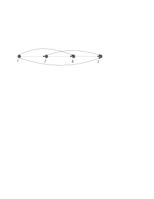
Next, consider the four node link shown in Fig. 9(b). For this linear deployment we assume . For node to communicate with node , the message packet can be routed in four ways as shown in Fig. 9(b). An analytical expression for the probability of path failure is tedious, so instead we simulate the network shown in Fig. 9(b) in both the correlated and i.i.d. link shadowing. We take samples of the normalized received powers under both correlated shadowing and i.i.d shadowing models. We then determine from the result the probability that there is no path from node to node .
VII-C Discussion
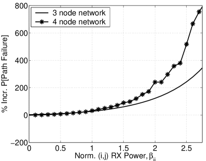
We compare the probability of path failure between node and node for both the cases of i.i.d. and correlated link shadowing in Fig. 10. The analysis shows that when a multi-hop network is designed for , then the probability of path failure is 120% greater in correlated shadowing as compared to i.i.d. shadowing. Increasing the reliability of the network by designing it for higher only increases the disconnect between the two models. It is only when we design the network for very unreliable links (e.g., , for which link is connected 1/2 the time) that the models have a similar result. Clearly, path connectivity is much more likely under the i.i.d. model than under the realistic correlated link shadowing model.
The four-node example shows that as paths become longer, it becomes increasingly important to consider correlated link shadowing. While the 3-node network had a 120% increase in probability of path failure, the 4-node network showed a 200% increase in the same probability. While Figure 10 show the results up to , higher values correspond to higher reliability links, and reliable networks will be designed with even higher link margins. When networks are designed for high reliability, the effects of ignoring link correlations are dramatic.
VIII Conclusion
A statistical joint path loss model for multi-hop (sensor, ad hoc, and mesh) networks is presented that relates the shadow fading on different links in a multi-hop network to the underlying shadowing field caused by an environment of deployment. A network channel measurement system is used to measure a multi-hop network deployed in an ensemble of environments. The data set is used to demonstrate and quantify statistically significant shadowing correlations among different geometries of links. The measured correlations agree with the proposed model, and can be applied to a greater variety of links than possible using an existing correlated shadowing model. Finally, this paper analyzes path connectivity in simple multi-hop networks to show the importance of the consideration of shadowing correlation when designing reliable networks. The probability of path failure is underestimated by a factor of two or higher by the current i.i.d. shadowing model.
Future work will test other ensembles of deployments, both indoors and outdoors. The effects of correlated shadowing will have impact on higher layer networking protocols and algorithms, and in interference and multiple-access control, and future work will quantify this intuition.
APPENDIX
Here we present the derivation of the probability in (29). From (21), we can note that , and are joint Gaussian random variables. Thus the conditional distributions, and , are Gaussian. The links and in Fig. 9 are observed to have very small or no correlation between them. Thus the joint distribution, , can be approximated as:
| (30) |
The joint distribution of , and is:
| (31) |
The probability can be written in terms of joint distributions as:
| (32) | |||||
where,
The square in the RHS of (32) comes from the fact that for the link geometry considered, .
References
- [1] H. Lee, A. Cerpa, and P. Levis, “Improving wireless simulation through noise modeling,” in Information Processing in Sensor Networks (IPSN’07), April 2007.
- [2] G. Marconi, “Wireless telegraphy,” Journal of the IEE, vol. 28, pp. 273–315, 1899.
- [3] H. Hashemi, “The indoor radio propagation channel,” Proccedings of the IEEE, vol. 81, no. 7, pp. 943–968, july 1993.
- [4] T. Rappaport, Wireless Communication : principles and Practice, 2nd ed. Printice Hall, 1996.
- [5] H. Bertoni, Radio Propagation for Modern Wireless Systems. Prentice Hall Professional Technical Reference, 1999.
- [6] C. Bettstetter and C. Hartmann, “Connectivity of wireless multihop networks in a shadow fading environment,” Wirel. Netw., vol. 11, no. 5, pp. 571–579, 2005.
- [7] R. Hekmat and P. V. Mieghem, “Connectivity in wireless ad-hoc networks with a log-normal radio model,” Mob. Netw. Appl., vol. 11, no. 3, pp. 351–360, 2006.
- [8] D. Kotz, C. Newport, and C. Elliott, “The mistaken axioms of wireless-network research,” Dept. of Computer Science, Dartmouth College, Tech. Rep. TR2003-467, July 2003. [Online]. Available: http://www.cs.dartmouth.edu/reports/abstracts/TR2002-467/
- [9] G. D. Durgin, Space-time Wireless Channel. Prentice Hall Communication Engineering and Emerging Technologies Series, 2004.
- [10] A. A. Saleh and R. A. Valenzuela, “A statistical model for indoor multipath propagation,” IEEE J. Sel. Areas in Communications, vol. 5, pp. 128–137, Feb. 1987.
- [11] G. Malmgren, “On the performance of single frequency networks in correlated shadow fading,” IEEE Trans. Broadcasting, vol. 43, no. 2, pp. 155–165, June 1997.
- [12] K. S. Butterworth, K. W. Sowerby, and A. G. Williamson, “Base station placement for in-building mobile communication systems to yield high capacity and efficiency,” IEEE Trans. Communications, vol. 48, no. 4, pp. 658–669, April 2000.
- [13] T. Klingenbrunn and P. Mogensen, “Modelling cross-correlated shadowing in network simulations,” in IEEE VTC 1999, vol. 3, Sept. 1999, pp. 1407–1411.
- [14] J. Zhang and V. Aalo, “Effect of macrodiversity on average-error probabilities in a Rician fading channel with correlated lognormal shadowing,” IEEE Trans. Communications, vol. 49, no. 1, pp. 14–18, Jan. 2001.
- [15] A. Safak and R. Prasad, “Effects of correlated shadowing signals on channel reuse in mobile radio systems,” IEEE Trans. Vehicular Technology, vol. 40, no. 4, pp. 708 – 713, Nov. 1991.
- [16] M. Gudmundson, “Correlation model for shadow fading in mobile radio systems,” IEEE Elecronics Letters, vol. 27, no. 23, pp. 2145–2146, November 1991.
- [17] Z. Wang, E. K. Tameh, and A. Nix, “Simulating correlated shadowing in mobile multihop relay/ad-hoc networks,” IEEE 802.16 Broadband Wireless Access Working Group, Tech. Rep. IEEE C802.16j-06/060, July 2006.
- [18] N. Patwari, Y. Wang, and R. O’Dea, “The importance of the multipoint-to-multipoint indoor radio channel in ad-hoc networks,” IEEE Wireless Communication and Networking Conference (WCNC), Orlando FL, March 2002.
- [19] “Mpr-mib users manual,” Crossbow Technology Inc, June 2006, revision B.
- [20] A. Coulson, A. G. Williamson, and R. G. Vaughan, “A statistical basis for lognormal shadowing effects in multipath fading channels,” IEEE Trans. on Veh. Tech., vol. 46, no. 4, pp. 494–502, April 1998.
- [21] W. W. Hines and et.al., Probability and statistics in Engineering, 4th ed., 2003.
- [22] K. Worsley, A. Evans, S. Strother, and J. Tyler, “A linear spatial correlation model, with applications to positron emission tomography,” Journal of the American Statistical Association, vol. 86, no. 413, pp. 55–67, March 1991.
- [23] P. Agrawal and N. Patwari. Matlab code for public download. [Online]. Available: http://span.ece.utah.edu
(a)  (b)
(b) 
| Correlation with Measured Data | |
|---|---|
| Proposed Model | 0.804 |
| Gudmundson’s Model | 0.644 |
(a) 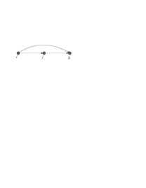 (b)
(b) 