Outliers from the Mass–Metallicity Relation I: A Sample of Metal-Rich Dwarf Galaxies from SDSS

Abstract

We have identified a sample of 41 low-mass high–oxygen abundance outliers from the mass–metallicity relation of star-forming galaxies measured by Tremonti et al. (2004). These galaxies, which have $8.6<12+\log(\mbox{O}/\mbox{H})<9.3$ over a range of $-14.4>M_{B}>-19.1$ and $7.4<\log(\mbox{M}_{\star}/\mbox{M}_{\odot})<10$, are surprisingly non-pathological. They have typical specific star formation rates, are fairly isolated and, with few exceptions, have no obvious companions. Morphologically, they are similar to dwarf spheroidal or dwarf elliptical galaxies. We predict that their observed high oxygen abundances are due to relatively low gas fractions, concluding that these are transitional dwarf galaxies nearing the end of their star formation activity.

1. Introduction

There is a well-known positive correlation between galaxy luminosity and metallicity (Lequeux et al., 1979; Garnett & Shields, 1987). Tremonti et al. (2004) measured this relation for 53400 star-forming galaxies from the Sloan Digital Sky Survey (SDSS) Data Release 4 (DR4, Adelman-McCarthy et al. 2006), estimating the gas phase oxygen abundance, $12+\log(\mbox{O}/\mbox{H})$, from H II region emission lines as the surrogate for “metallicity.” Using estimates of the galaxy stellar masses derived from the techniques of Kauffmann et al. (2003), Tremonti et al. showed that metallicity is better correlated with galaxy mass than with luminosity, which suggests that the observed relation arises from the fact that lower mass galaxies have lower escape velocities than higher mass galaxies and so lose metals more easily via, e.g., supernova winds (Larson, 1974). However, Dalcanton (2007) showed that even if a low-mass galaxy can selectively remove its metals via winds, subsequent star formation can essentially erase the effects on the gas-phase metallicity; both a low star formation rate and a large gas fraction are needed to retain low metal abundances. Other proposed origins for the mass–metallicity relation include lower star formation rates in less massive galaxies giving rise to fewer massive stars and therefore less metal production (Köppen et al., 2007).

Despite the locus of galaxies in the mass–metallicity plane having intrinsically high scatter (e.g., a 1-$\sigma$ spread of $\pm 0.15$ dex in $12+\log(\mbox{O}/\mbox{H})$ at $9.5<\log(\mbox{M}_{\star}/\mbox{M}_{\odot})<9.6$), in the absence of good quality spectra it has become an increasingly common practice to deduce or assign metallicities to galaxies based simply on their luminosities. In particular, the idea persists that dwarf galaxies are always “metal-poor,” certainly a fair assumption in the Local Group. In this study however, we will show that there is a significant population of low-mass galaxies with high gas-phase oxygen abundances relative to the mass–metallicity relation defined by Tremonti et al. (2004); high-mass low-metallicity outliers from the mass–metallicity relation will be the focus of an upcoming paper. As shown in Figure 1, we find 24 galaxies with $-17\gtrsim M_{B}\gtrsim-19$ mag and $12+\log(\mbox{O}/\mbox{H}\gtrsim 9$ and 17 high-metallicity outliers with $M_{B}>-17$ mag. We explain how we selected this sample in § 2 and verified the galaxies’ high oxygen abundances in § 2.3. In § 3 we discuss some of the possible explanations for the existence of such a population of galaxies and explain why we predict that these galaxies should have relatively low gas masses. Specifically, in § 3.4 we discuss the evidence for our galaxies being so-called “transition” dwarf galaxies. Finally, we summarize our results and conclusions in § 4.

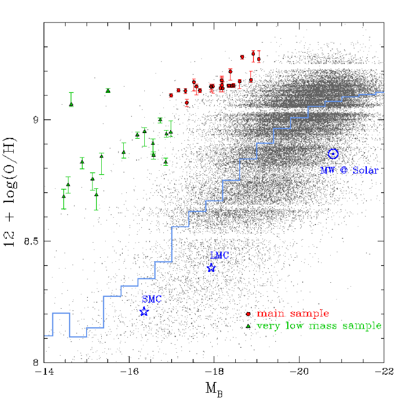
Figure 1.— $12+\log(\mbox{O}/\mbox{H})$ vs. $M_{B}$, with $\log(\mbox{O}/\mbox{H})$ taken from Tremonti et al. (2004) and $M_{B}$ measured using the methods of Assef et al. (2008). The small grey points are star-forming galaxies with SDSS magnitude errors $<0.1$ mag; the red circles are the 24 galaxies in our main sample, and the green triangles are the very low mass sample. The errorbars on $12+\log(\mbox{O}/\mbox{H})$ show the central 68% spread from Tremonti et al. (2004). The pale blue histogram denotes the median $12+\log(\mbox{O}/\mbox{H})$ in bins of $M_{B}$ with width $\Delta M_{B}=0.4$ mag; these medians are probably artificially high at low luminosities due to substantial contamination at high $12+\log(\mbox{O}/\mbox{H})$ as discussed in § 2.2. The Milky Way, SMC, and LMC are shown using $M_{B}$ from Karachentsev (2005), and the $12+\log(\mbox{O}/\mbox{H})$ measurements are as discussed in the § 2.

2. Finding Outliers from the Mass–Metallicity Relation

We began with the sample of $\sim 110000$ star-forming galaxies with measured gas-phase oxygen abundances and stellar masses from Tremonti et al. (2004). High-metallicity outliers from the mass–metallicity locus can be due to main three causes, and our cuts were taken with these in mind. First, some galaxies can spuriously appear to be underluminous for their mass. Examples include highly inclined galaxies subject to strong internal extinction and H II regions in larger galaxies that SDSS has mistakenly flagged as a galaxy. Among relatively nearby galaxies (e.g., those in the Virgo cluster) some have large peculiar velocities relative to the Hubble flow, leading to a misestimation of their distance modulus and thus absolute magnitude. Secondly, rogue outliers can have spuriously high estimated metallicities; the galaxy, for example, may not be at high enough redshift to have the strongly constraining [O II] $\lambda 3727,9\,$Å emission line in the SDSS bandpass. Also, the strengths of the [O II] and [O III] lines paradoxically decrease with oxygen abundance, so at low signal-to-noise, the metallicity can be overestimated due to underestimated line fluxes. Finally, the object can be an honest outlier; these are the objects we want in our final sample. We found that a large number of cuts in different parameter spaces is useful for automatically rejecting many objects which would otherwise have to be thrown out by visual inspection. We ran two searches on the full Tremonti et al. sample for high-metallicity outliers. For the first, we were very conservative with our cuts so as to be certain that the remaining galaxies are both statistically significant and not spurious. However, due to significant contamination at low luminosities, this “main” sample has no members with $\log\mbox{M}_{\star}<9.15$. We therefore did a separate, less stringent search for the lowest luminosity outliers; to distinguish it from the main sample, we refer to this sample of lower mass galaxies as the “very low mass” sample.

Figure 1 shows where our sample falls in the $12+\log(\mbox{O}/\mbox{H})$–$M_{B}$ plane; all galaxy images are shown in Figure 2 and summary information is presented in Table 1. For reference, in Figure 1 we plot the Small and Large Magellanic Clouds and Milky Way using $M_{B}$ from Karachentsev (2005). We recalculated $12+\log(\mbox{O}/\mbox{H})$ for the SMC and LMC using the line ratios reported by Russell & Dopita (1990) of six H II regions in the SMC and four H II regions in the LMC and the relation $12+\log(\mbox{O}/\mbox{H})=9.37+2.03\times\mbox{N}2+1.26\times\mbox{N}2^{2}+0.32\times\mbox{N}2^{3}$, where $\mbox{N}2\equiv\log([\mbox{{N~{}II}}]\lambda 6584/\mbox{H}\alpha)$ (Pettini & Pagel, 2004; Kewley & Ellison, 2008). We then transformed these abundances onto the Tremonti et al. (2004) scale using the formulae given by Kewley & Ellison (2008), resulting in average metallicities of 8.21 and 8.39 for the SMC and LMC, respectively. The Milky Way is plotted also plotted for reference at the Solar oxygen abundance of 8.86 (Delahaye & Pinsonneault, 2006).

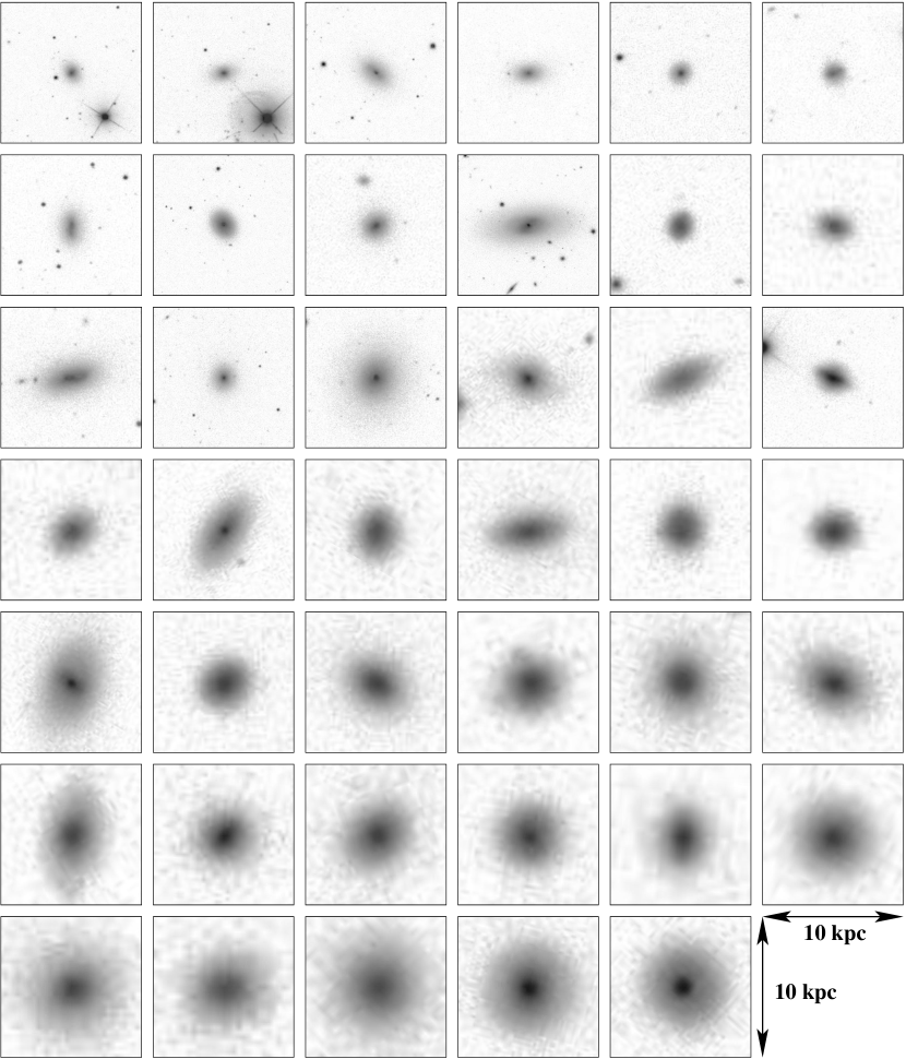
Figure 2.— SDSS images of high-metallicity dwarf galaxies scaled to $10\times 10$ kpc, with $M_{B}$ decreasing to the right and down from $-14.4$ to $-19.1$, so that the faintest galaxy is in the upper-left corner. The stellar masses for this sample range from $\log\mbox{M}_{\star}\approx 7.4$ to 9.9.

Table 1Full sample of low-luminosity mass–metallicity outliers

RA	dec	$12+\log(\mbox{O}/\mbox{H})$	$M_{B}$	$\log\mbox{M}_{\star}$	redshift	Notes
193.9056	$-1.32986$	8.68	$-14.46$	7.65	0.0029	blue core, IC 225
180.4589	$55.14507$	8.73	$-14.56$	7.73	0.0035
190.2097	$4.52583$	9.06	$-14.64$	7.39	0.0025	blue core, VCC 1855
179.0295	$64.35073$	8.83	$-14.89$	8.06	0.0047
228.0340	$1.58571$	8.76	$-15.14$	8.21	0.0065
126.6407	$25.49979$	8.69	$-15.23$	8.07	0.0072
227.2679	$0.82197$	8.85	$-15.35$	8.17	0.0055
193.6735	$2.10447$	9.12	$-15.50$	8.40	0.0029	bright core
126.6633	$25.59821$	8.86	$-15.87$	8.59	0.0078
208.3607	$5.20778$	8.94	$-16.19$	8.64	0.0027	blue core
128.5841	$50.45248$	8.95	$-16.36$	8.69	0.0114
40.3408	$0.05813$	8.90	$-16.56$	8.70	0.0227
212.9768	$53.93956$	8.85	$-16.57$	8.81	0.0064	blue core
190.5886	$2.06662$	9.00	$-16.73$	8.40	0.0044	bright core
36.6179	$1.16053$	8.82	$-16.86$	7.92	0.0051	blue core
117.1775	$26.53979$	8.94	$-16.88$	9.08	0.0155
182.7831	$0.95682$	8.95	$-16.98$	9.13	0.0206
133.8883	$31.21168$	9.10	$-16.99$	9.29	0.0068
25.7673	$14.52434$	9.12	$-17.16$	9.25	0.0284
225.5670	$38.80631$	9.12	$-17.32$	9.45	0.0147	bright core
142.9797	$39.27156$	9.07	$-17.36$	9.35	0.0275
139.3797	$33.47552$	9.15	$-17.52$	9.46	0.0221
202.2088	$-0.90846$	9.14	$-17.58$	9.26	0.0217
39.0487	$-7.73400$	9.12	$-17.66$	9.16	0.0314
143.4695	$41.07965$	9.14	$-17.92$	9.54	0.0145	bright core
187.1760	$44.09813$	9.13	$-17.93$	9.35	0.0239
182.8574	$44.43604$	9.14	$-17.97$	9.52	0.0231
211.3199	$54.20347$	9.13	$-18.15$	9.54	0.0417
258.4301	$57.18840$	9.16	$-18.18$	9.61	0.0290
208.9341	$4.24367$	9.14	$-18.19$	9.68	0.0295
227.6711	$41.16220$	9.13	$-18.20$	9.61	0.0316
352.8635	$13.90885$	9.14	$-18.34$	9.74	0.0324
206.4402	$63.85402$	9.14	$-18.36$	9.58	0.0313
153.2177	$12.34451$	9.20	$-18.39$	9.57	0.0315
177.7870	$49.69415$	9.14	$-18.41$	9.41	0.0482
144.1848	$33.91996$	9.14	$-18.45$	9.71	0.0426
162.6325	$0.36061$	9.16	$-18.60$	9.68	0.0384
195.6390	$-3.33894$	9.26	$-18.66$	9.55	0.0471
235.5660	$51.73211$	9.16	$-18.87$	9.83	0.0425
163.2191	$43.42840$	9.27	$-18.92$	9.90	0.0242
245.3673	$40.20360$	9.25	$-19.05$	9.91	0.0285	blue core

Note. — Sample of metal-rich dwarf galaxies, sorted by $M_{B}$. First sixteen lines (above the horizontal line) are the very low mass ($\log[\mbox{M}_{\star}/\mbox{M}_{\odot}]<9.1$) sample. RA and dec are in degrees, $12+\log(\mbox{O}/\mbox{H})$ and stellar mass from Tremonti et al. (2004), and $M_{B}$ is measured using the low-resolution templates of Assef et al. (2008) and corrected where necessary for peculiar velocities, as discussed in § 2; redshifts are spectroscopic redshifts and have not been corrected for peculiar velocities.

2.1. Main Sample Selection

Table 2 summarizes our selection of the main sample of 24 metal-rich low-mass galaxies. Spiral galaxies are known to have radial metallicity gradients such that the nuclear abundances are higher than averages over whole galaxies. Thus, if only a small fraction of the galaxy is within the SDSS spectroscopic $3\arcsec$ diameter fibers, the measured metallicity can appear to be artificially high relative to other galaxies. Following Tremonti et al. (2004), we make an initial cut by requiring that the fraction of the galaxy covered by the fiber to be greater than 10%. (In our final cut, we follow Michel-Dansac et al. (2008) and change this lower bound to 20%, which only eliminates two of the galaxies contained in the penultimate sample listed in Table 2.) We wanted the sample to be statistically significant, so outliers were then determined via a series of cuts in the $12+\log(\mbox{O}/\mbox{H})$ versus absolute $B$-band magnitude ($M_{B}$), $g$-band ($M_{g}$), and stellar mass (M_⋆) planes, as demonstrated with M_⋆ in Figure 3. For example, we divided the 52477 objects with SDSS magnitude errors $<0.1$ mag in all bands into bins of $M_{B}$ of width $\Delta M_{B}=0.4$ mag; in each bin we kept the 2.5% with the highest $12+\log(\mbox{O}/\mbox{H})$. We likewise took bins of $12+\log(\mbox{O}/\mbox{H})$ of width 0.1 dex and kept 2.5% of the objects with the faintest $M_{B}$. Similar cuts were made with $M_{g}$ (binsize $\Delta M_{g}=0.4$ mag) and $\log\mbox{M}_{\star}$ (binsize of $\Delta\log\mbox{M}_{\star}=0.1$ dex). $M_{g}$ was calculated from the SDSS $g$-band magnitude and the spectroscopic redshift, $M_{B}$ was calculated using the low-resolution spectral templates of Assef et al. 2008, and the stellar masses from the Tremonti et al. sample were measured using a combination of SDSS colors and spectra as described by Kauffmann et al. (2003). Only 58 objects survived this series of cuts.

At this point, we made a redshift cut: galaxies must have $z>0.024$ in order to have the [O II] $\lambda\lambda 3727,9$Å emission line pair in their SDSS spectrum, and as this is a highly constraining line for the metallicity, we determined that it should be in the spectrum in order to remove a possible source of systematics and so that we can measure the metallicity with a diagnostic that uses this line. Seven $z<0.024$ galaxies pass our subsequent $12+\log(\mbox{O}/\mbox{H})$ error and visual inspection cuts; after studying their spectra, as discussed below, we chose to keep these galaxies in our main sample. We also forced the cited $\pm 1\,\sigma$ error in $12+\log(\mbox{O}/\mbox{H})$ to be less than 0.05 dex; metallicities with large uncertainties are obviously more likely to be spurious than ones with small uncertainties. Unsurprisingly, the $z>0.024$ redshift cut (after all of the other cuts) also removed any galaxies with fiber fractions $<0.1$ which would have survived to that stage. We find, however, that this large number of cuts in various parameter spaces dramatically reduced the number of objects that had to be removed “by eye.” The final visual-inspection cut removed only two objects with nearby potential photometric contaminations. Finally, we re-examined the fiber fraction cut; following Michel-Dansac et al. (2008) we allowed the lower-limit fiber fraction to be 20% (excluding two objects from the sample). The final exclusion was a barred galaxy with a diameter of $\sim 10$″; the SDSS fiber size is $3\arcsec$, but this galaxy is labeled as having a fiber fraction of $\sim 60$%. This galaxy probably has spuriously low SDSS Petrosian magnitudes. The 24 galaxies in this main sample have a range of fiber fractions between 25% and 60% and a redshift range of $0.007<z<0.048$.

Table 2Cuts for Main Sample Selection

Cut	Number Surviving
Fiber fraction $>0.1$	107992
$k$-corrected SDSS magnitude errors $<0.1$ mag	48327
97.5% large (O/H) and small $M_{B}$	227
97.5% large (O/H) and small $M_{g}$	202
99% large (O/H) w.r.t. $M_{B}$	87
99% large (O/H) w.r.t. M⋆	66
97.5% small M⋆ w.r.t. (O/H)	51
redshift $>0.024$ for [O II]	34
$12+\log(\mbox{O}/\mbox{H})$ error $<0.05$ dex	22
Visual inspection	20
Fiber fraction $>0.2$ and photometry	17
redshift $z<0.024$ but surviving subsequent cuts	$7$

Note. — See § 2.1 and Figure 3 for a more detailed explanation.

Figure 3.— Zoomed in portion of the $12+\log(\mbox{O}/\mbox{H})$ vs. $\log\mbox{M}_{\star}$ plane with 97.5% (solid blue line and short dashed cyan line) and 99% (long dashed light blue line) cuts shown; see § 2.1 and Table 2. The black points have SDSS magnitude errors $<0.1$ mag and the red points are the 24 galaxies in our main sample, which are similar in luminosity to the Large Magellanic Cloud (which has a $12+\log(\mbox{O}/\mbox{H})$ of 8.39). The errorbars on $12+\log(\mbox{O}/\mbox{H})$ show the central 68% spread from Tremonti et al. (2004).

2.2. Very Low Mass Sample Selection

It is obvious from Figure 1 that the selection of our main sample artificially imposes a lower mass cutoff. This does not mean that there is not a statistically significant sample of interesting galaxies with $M_{B}>-17$; it just means that there are more contaminating objects with measured high metallicities in the low-luminosity regime than at brighter magnitudes. That is, the most extreme outliers with $M_{B}<-17$ in one parameter space (e.g., the $12+\log(\mbox{O}/\mbox{H})$ vs. $M_{B}$ plane) are not also outliers in one of the others (e.g., the $12+\log(\mbox{O}/\mbox{H})$ vs. $\log\mbox{M}_{\star}$ plane). The true very low luminosity mass–metallicity outliers therefore have lower abundances than these spurious outliers. We therefore did a separate search for high-metallicity galaxies at extremely low luminosities and masses, as summarized in Table 3. We chose to not apply a fiber fraction cut for this sample because lower luminosity galaxies are preferentially closer and therefore subtend a larger angle on the sky, making it more difficult for a substantial fraction of the galaxy to be within the 3″ SDSS fiber diameter. We therefore began the selection with a magnitude error cut, like the one for the main sample. We also removed objects with fiber fractions $>0.2$ occupying the parameter space already excluded by the main sample: any objects with $M_{B}$ brighter than $-17$ mag, $\log\mbox{M}_{\star}>9.15$, and a high $\log(\mbox{O}/\mbox{H})$ at the 95% level with respect to M_⋆ were excluded. The cuts in $12+\log(\mbox{O}/\mbox{H})$ relative to $M_{B}$, $M_{g}$ and M_⋆ are all less stringent than for the main sample, but because for this sample we are interested in the very low mass objects, we took a strong (99% level) cut in M_⋆ relative to $12+\log(\mbox{O}/\mbox{H})$. Six galaxies were excluded due to metallicity re-estimation considerations (as discussed below). Three of the remaining galaxies are potentially members of the Virgo cluster; of these, only two remain clear outliers from the $M_{B}$–metallicity locus when their distance moduli are shifted to the Virgo value of $30.74$ magnitudes (Ebeling et al., 1998). (We do not attempt to correct the stellar mass estimates due to the effects of peculiar velocity.) Finally, the 95% high (O/H) with respect to $M_{g}$ cut excludes the galaxy IC 225 from the sample, which is pointed out by Gu et al. (2006) to have a relatively high metallicity and a compact blue core. As this galaxy passes all of the other cuts and is clearly interesting, we added it back to the sample, raising the total number of galaxies in the very low mass sample to 17 and the full sample to 41. The very low mass sample has fiber fractions ranging from 0.04 to 0.45; more than half of the 17 galaxies in this sample have fiber fractions below 0.1 and only 5 are above 0.2. Also, none of these galaxies would have survived the main sample redshift cut, as the very low mass galaxies occupy the redshift range $0.00249<z<0.0227$, with the most nearby objects being only $\sim 12$ Mpc away.

Table 3Cuts for Very Low Mass Sample Selection

Cut	Number Surviving
$k$-corrected SDSS magnitude errors $<0.1$ mag	52744
84% high (O/H) w.r.t. $M_{B}$	8405
$M_{B}>-17$ mag	217
$\log\mbox{M}_{\star}<9.15$	201
84% high (O/H) w.r.t. M⋆	192
$12+\log(\mbox{O}/\mbox{H})$ error $<0.05$ dex	139
99% low $\log\mbox{M}_{\star}$ w.r.t. (O/H)	105
exclude 95% high (O/H) w.r.t. M⋆, fiber fraction $>0.1$	78
95% high (O/H) w.r.t. $M_{g}$	32
Visual inspection	23
Metallicity comparison	17
Absolute magnitude correction	16

Note. — See § 2.2 and Figure 3 for a more detailed explanation. The 95% high (O/H) w.r.t. $M_{g}$ cut excludes IC 225, which passes subsequent cuts and is nonetheless included in plots and discussions. Note lack of fiber-fraction cut.

2.3. Measuring High Oxygen Abundances

Are these 41 galaxies true outliers from the mass–metallicity relation, or are they just the tail of the scatter of the Tremonti et al. (2004) measurements? As a first check, the galaxies fall where expected on the standard Baldwin, Phillips, & Terlevich (BPT) diagrams for $\log(\mbox{[{O~{}III}]}\,\lambda 5007/\mbox{H}\beta)$ vs. $\log(\mbox{[{N~{}II}]}\,\lambda 6548/\mbox{H}\alpha)$ and $\log(\mbox{([{S~{}II}]}\,\lambda\lambda 6717+31)/\mbox{H}\alpha)$ (Baldwin et al., 1981; Kewley et al., 2006). We note that there are several complications with measuring high metallicities using visible wavelength spectra (see Bresolin 2006 for a thorough review). The main problem is that cooling is more efficient at high metallicities, which translates into lower nebular temperatures and hence weaker [O II] and [O III] visible-wavelength lines, with the primary cooling load shifting to the far-infrared fine structure emission lines that cannot be readily observed. The result is that at high abundances the visible wavelength spectra become increasingly insensitive to changes in $\log(\mbox{O}/\mbox{H})$. In fact, some diagnostics, like the traditional R₂₃ line index, effectively saturate at high metallicity (Kewley & Ellison, 2008), making it rather difficult to accurately measure even relative abundances. Because we would like to verify the high estimated oxygen abundances and we cannot reproduce the Tremonti et al. abundance calculations, which are based on a Bayesian statistical method, we measured $\log(\mbox{O}/\mbox{H})$ in our galaxies using two recommended methods from Kewley & Ellison (2008).

Another possible source of systematic inaccuracy in the abundance estimates is the treatment of extinction corrections. The corrections traditionally applied use the H I Balmer decrement and assume a simple uniform foreground obscuring screen model like that used for stars to estimate $A_{V}$ and correct the other emission lines. It is expected, however, that extinction towards extended sources like H II regions is better described as a clumpy screen, for example the turbulent screen models of Fischera & Dopita (2005). In these, use of a simple screen tends to systematically overestimate the extinction correction for the O II $\lambda\lambda$3727,29Å emission line, leading to a systematic underestimate of the gas-phase oxygen abundance. In all of our galaxies the H I Balmer decrement measurements are consistent with low $A_{V}$ ($\lesssim 0.5$) for a simple screen extinction model, so this is not a big effect compared to other sources of measurement error given the attenuation curves in Fischera & Dopita (2005).

Kewley & Ellison have measured the gas-phase metallicities in star forming galaxies from SDSS using ten different methods, including that of Tremonti et al. (2004); they also provide average relations relating each pair of methods. While no one metallicity estimate is strictly believable—i.e., the true Oxygen-to-Hydrogen ratio—the relative measurements are generally robust (Kewley & Ellison, 2008). Using the Data Release 6 SDSS spectra (Adelman-McCarthy et al., 2008), we subtracted the underlying stellar continuum using the STARLIGHT program (Cid Fernandes et al., 2005). We then calculated $12+\log(\mbox{O}/\mbox{H})$ using the revised Kewley & Dopita (2002) method given in Equation (A3) of Kewley & Ellison (2008),

$$\log(\mbox{[{N~{}II}]}/\mbox{[{O~{}II}]}) = 1106.8660-532.1451Z+96.37326Z^{2}$$ (1)

$$-7.8106123Z^{3}+0.32928247Z^{4},$$

where $Z\equiv 12+\log(\mbox{O}/\mbox{H})$. Like Kewley & Ellison, we found the roots of this equation using the fz_roots program in IDL. We also measured the metallicity using the “O3N2” method of Pettini & Pagel (2004), as recommended by Kewley & Ellison, where

$$12+\log(\mbox{O}/\mbox{H})=8.73-0.32\times\log\left(\frac{[\mbox{{O~{}III}}]\lambda 5007/\mbox{H}\beta}{\mbox{[{N~{}II}]}\,\lambda 6584/\mbox{H}\alpha}\right).$$ (2)

We choose to not use the R₂₃ diagnostic for measuring $12+\log(\mbox{O}/\mbox{H})$ because it is known to be difficult to calibrate at these abundances (Kewley & Dopita, 2002). In particular, while the seventeen $z>0.024$ galaxies in our main sample span $\sim 0.2$ dex on the Tremonti et al. scale, they span $\sim 0.6$ dex when their metallicities are calculated using the R₂₃ methods of either McGaugh (1991) or Zaritsky et al. (1994), reflecting the fact that the R₂₃ parameter essentially saturates at high oxygen abundances (Bresolin, 2007).

The oxygen abundances for our 41 galaxies plotted against these adopted metallicities in Figure 4. The dotted line indicates equal measurements; the other two lines are the empirically determined relations from Kewley & Ellison. The galaxies in our sample fall preferentially above the relation for the Pettini & Pagel method, but surprisingly those galaxies for which it is measurable fall below the relation for the Kewley & Dopita method. One possible explanation for this discrepancy is that because [O II] and [N II] are widely separated in wavelength, a misestimation of the extinction or a poorly fitted continuum (especially for the weak [O II] emission line) can lead to underestimated abundances. Specifically, there is often a degeneracy when fitting the stellar continuum between the extinction and the stellar population. While the continuum fitting for our spectra are fairly good (i.e., they exhibit low residuals after the stellar template is subtracted), we tested the sensitivity to the continuum level at [O II] $\lambda 3727$Å by calculating the Kewley & Dopita metallicity when the continuum is over- and underestimated; the mean of these two extreme metallicities is still systematically larger than expected by the mean relation, implying that the shift is not due to continuum fitting error. We quantify the differences between the Pettini & Pagel and Kewley & Dopita methods by examining the product of the vertical displacement of each galaxy (for an optimally fit continuum) from the two Kewley & Ellison relations; only one galaxy in the main sample has a significantly high Tremonti et al. metallicity relative to both of the other indicators. However, this $12+\log(\mbox{O}/\mbox{H})$ was still high enough that even when the Tremonti et al. metallicity was replaced with the one expected from either relation, the galaxy still passes the cuts in both the $M_{g}$- and M_⋆-metallicity planes. While the $z<0.024$ galaxies do not have measurable [O II] (and hence we cannot use the Kewley & Dopita diagnostic for them), the low redshift sample occupies a similar part of the Tremonti et al. versus Pettini & Pagel parameter space as the galaxies in the main sample. For the very low-mass sample of galaxies, out of the 22 galaxies which passed our visual inspection test, we excluded 6 because they were more than $0.1$ dex above the Pettini & Pagel relation from Kewley & Ellison; this is actually a more stringent cut than used for the main sample because several of the galaxies in the main sample with $>0.1$ dex deviations from the Pettini & Pagel relation have compensating negative deviations relative to the Kewley & Dopita scale. We interpret these results to mean that the 41 galaxies we have identified are true high-metallicity low-mass outliers from the mass–metallicity relation.

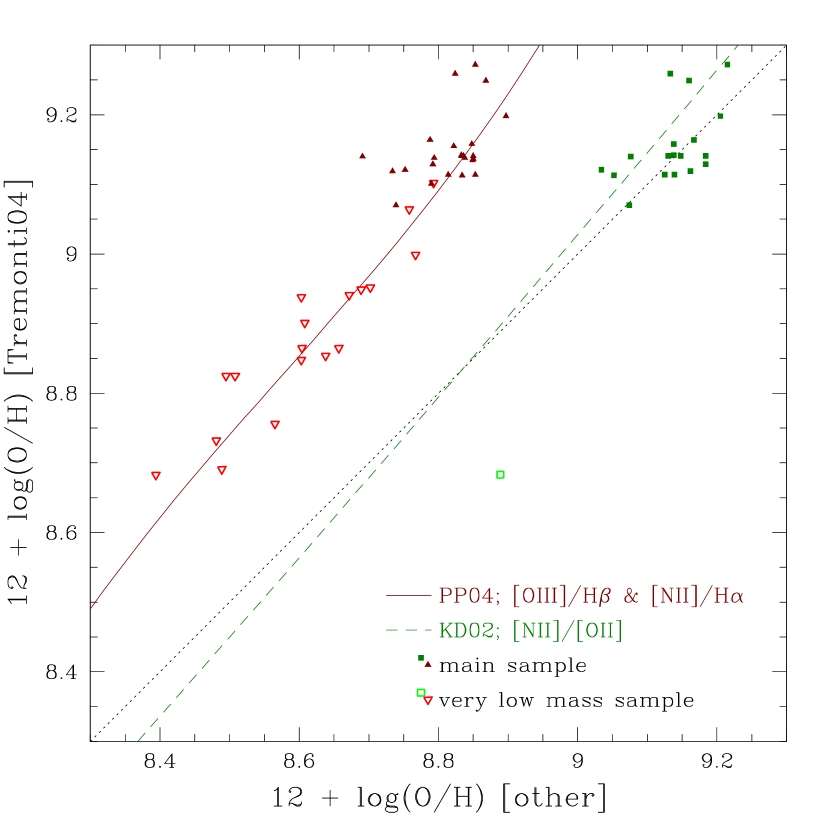
Figure 4.— Comparisons of oxygen abundances of low-luminosity mass–metallicity outliers measured with different methods as compared to mean relations. The red triangles denote abundances measured with the method of Pettini & Pagel (2004); the green squares are metallicities from revised Kewley & Dopita (2002) method from Kewley & Ellison (2008). The red solid line and green dashed lines are the conversion from the Pettini & Pagel (2004) method and the Kewley & Dopita (2002) method to the Tremonti et al. (2004) metallicity respectively; the black dotted line indicates equal measurements. Conversions are from Kewley & Ellison (2008); see § 2.3 for a more in depth discussion.

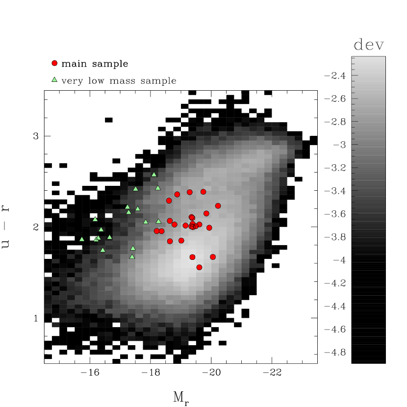
Figure 5.— High-metallicity low-mass galaxies on the color–magnitude diagram ($u-r$ vs. $M_{r}$) from the flux-limited $z<0.06$ sample of Unterborn & Ryden (2008). The color scale on the right shows the $\log f$ of each bin, where $f$ is the fraction of galaxies in that bin; bin sizes are $0.05$ mag in $u-r$ and $0.25$ in $M_{r}$. The red circles denote the 24 galaxies from the main sample and the green triangles denote the 17 galaxies in the very low mass sample.

3. Discussion

The 41 dwarf galaxies selected as described in § 2 are surprisingly non-pathological. They have undisturbed stellar morphologies (see Figure 2). Furthermore, given that by selection these galaxies have both low luminosities and high metallicities and that there is a trend for redder, brighter galaxies to have higher oxygen abundances (see, e.g., Cooper et al. 2008) these metal-rich dwarfs do not occupy unexpected region of the color–magnitude diagram (see Figure 5 and also § 3.4). How, then, did they come to have such high oxygen abundances? One obvious possibility is that these metallicities are due to an environmental effect, but as we describe in § 3.1, the galaxies in our sample are non-interacting and rather isolated. Though several models predict that these galaxies should have high specific star formation rates, we show in § 3.2, that these galaxies have normal star formation rates for their masses. We explain in § 3.3 why we predict that these metal-rich dwarf galaxies should have relatively low gas fractions, and we discuss the implications of this prediction in the broader context of transition-type dwarf galaxies in § 3.4.

3.1. Environment

While the origin of scatter in the mass–metallicity relation is unknown, one popular proposal is that environment affects metallicity. Recently, Michel-Dansac et al. (2008) studied close pairs of star-forming galaxies in SDSS with projected separations of $<100\,$kpc and radial velocity separations of $<350\,$km s^-1. Their results indicate that for minor mergers, the less massive galaxy is likely to be preferentially more metal rich than predicted by the mass–metallicity relation. Likewise, Cooper et al. (2008), after accounting for correlations within the color–magnitude diagram, find a strong positive correlation between metallicity and overdensity for $0.05<z<0.15$ SDSS-selected star-forming galaxies that can account for up to $\sim 15$% of the scatter in the mass–metallicity relation. In light of these results, we searched for nearby neighbors of the seventeen $z>0.024$ main sample metal-rich dwarf galaxies in a cylindrical volume of depth $\pm 1000$ km s^-1 and projected radius of 1 Mpc. We find that our galaxies are relatively isolated; none of them would have made it into the Michel-Dansac et al. (2008) sample. Seven out of these seventeen galaxies in our sample have no neighbors within this volume. Of the 10 remaining galaxies, four have no neighbors within 500 km s^-1 and 500 kpc, and only two have any neighbors within 500 km s^-1 and 100 kpc. One of these two seems to be on the outskirts of a nearby cluster, but it is unclear whether or not it is physically associated with the cluster (and there is only one small, faint, non-star-forming galaxy within the Michel-Dansac et al. volume). The other galaxy with a nearby neighbor is $\sim 400$ km s^-1 and 85 kpc from a less-massive relatively metal-poor ($12+\log[\mbox{O}/\mbox{H}]\approx 8.6$) star-forming galaxy. We therefore conclude that interactions with neighbors do not explain the observed high abundances of our main sample of $\log\mbox{M}_{\star}\sim 9.5$ galaxies.

The galaxies in the very low mass sample (as well the $z<0.024$ galaxies in the main sample), however, are generally at low enough redshift that an automated search for neighbors in velocity and projected distance space is difficult. Like the galaxies in the main sample, none of the lower-mass galaxies are in obviously interacting systems. Only one has an clear companion; it is a $\log\mbox{M}_{\star}=9.13$ galaxy which appears to be a satellite of a non-starforming companion 33 kpc and $\sim 120$ km s^-1 away. Also, while two of the seventeen galaxies in the very low mass sample may be in the Virgo cluster, clearly a rich environment cannot explain the high oxygen abundances observed in all of these galaxies.

3.2. Star Formation Rates

Dalcanton (2007) finds that for a galaxy to have a low metallicity, it must have both a low star formation rate and a high gas fraction; she argues that the observed low star formation efficiency in galaxies with circular velocities $\lesssim 120$ km s^-1 can explain the mass–metallicity relation. Köppen et al. (2007) similarly suggest that the mass–metallicity relation could be due to a mass–star formation rate relation: a galaxy with a lower rate of star formation will have relatively fewer massive stars, and therefore a lower oxygen abundance. In either of these scenarios, we might expect the mass–metallicity outliers to have high star formation rates for their masses. On the other hand, Ellison et al. (2008) find that at low stellar masses, galaxies with higher specific star formation rates tend to have lower oxygen abundances. As Figure 6 shows, the galaxies in the main sample do not have preferentially high or low instantaneous specific star formation rates, while typical star formation rates for the the very low mass sample galaxies are $\sim 0.3$ dex lower than expected given their masses.

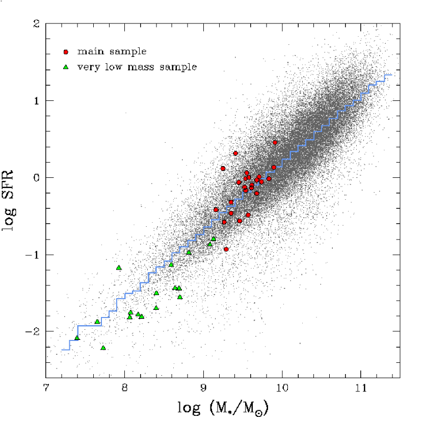
Figure 6.— Star formation rate vs. stellar mass. The grey points are galaxies from the Tremonti et al. (2004) sample with SDSS magnitude errors $<0.1$ mag, the galaxies in our main sample are denoted with red circles, and the galaxies in our very low mass sample are marked with green triangles. The blue histogram denotes the median star formation rate in bins of $\log\mbox{M}_{\star}$ of width 0.1 dex. The star formation rates estimates are from (Brinchmann et al., 2004) and the stellar mass estimates are from Tremonti et al. (2004) and Kauffmann et al. (2003).

3.3. Effective Yields and Gas Fractions

So why do these galaxies have such high oxygen abundances? Consider a closed box star forming system (i.e., a system with no gas inflow or outflow). The metallicity $Z\equiv\;$(mass of metals in gas phase)/(total gas mass) is

$$Z=y\ln\left(\frac{1}{f_{\mbox{\scriptsize gas}}}\right),$$ (3)

where $f_{\mbox{\scriptsize gas}}\equiv M_{\mbox{\scriptsize gas}}/(M_{\star}+M_{\mbox{\scriptsize gas}})$ is the gas fraction and $y\equiv\;$(mass of metals in gas)/(mass of metals in stellar remnants and main sequence stars) is the metal yield. An immediately striking aspect of Equation 3 is that there is no implicit dependence on the total galaxy mass; the deviations from a universal metallicity observed via the mass–metallicity relation are presumably then due to the fact that galaxies are not scaled closed box versions of one another: variations of the yield with mass, a dependence on the gas fraction with mass, or a combination of these effects plays a role. For a galaxy to have a higher metallicity than other galaxies of the same mass, Equation 3 tells us that it must have either a relatively high yield or a relatively low gas fraction. Observationally, the yield—which depends on both star formation physics as well as gas inflow and outflow—is a difficult quantity to measure; one popular way to address this problem is to define an effective yield,

$$y_{\mbox{\scriptsize eff}}\equiv\left[\frac{Z_{\mbox{\scriptsize gas}}}{\ln(1/f{\mbox{\scriptsize gas}})}\right],$$ (4)

as the yield the galaxy would have were it actually a closed system. Given the galaxy’s metallicity and gas fraction, one can then easily calculate $y_{\mbox{\scriptsize eff}}$. A common explanation for the mass–metallicity relation is that the effective yield is positively correlated with galaxy mass, so that lower mass galaxies are able to preferentially lose metals to the intergalactic medium via winds because of their relatively shallow potential wells (see e.g., Larson, 1974; Finlator & Davé, 2008, and references therein). In particular, Tremonti et al. (2004) tested this idea by comparing effective yields and baryonic masses. However, because when estimating the effective yield from Equation 4, Tremonti et al. use the measured $12+\log(\mbox{O}/\mbox{H})$ values, outliers in the mass–metallicity relation are practically guaranteed to be outliers in the effective yield–baryonic mass relation.

Regardless, it is obvious from Equation 3 that our metal-rich dwarfs must either have unusually high yields or unusually low gas fractions for their masses. Galaxy yields can be affected by three processes: star formation, metal-deficient gas inflows, and metal-rich gas outflows. As shown in Figure 6 and discussed in § 3.2, we find that the star formation rates for this population of galaxies are consistent with those of other galaxies of similar masses. Dalcanton (2007) has shown that metal-poor gas inflow is insufficient to explain the typically low metal abundances of low-mass galaxies; we therefore conclude that a lower inflow rate is insufficient to explain the higher abundances of our galaxies. It is possible that these galaxies are less effective at driving outflows than other dwarfs. For example, Ellison et al. (2008) find that, at fixed mass, galaxies with smaller half-light radii tend to have higher abundances; this picture is consistent with the idea that it is more difficult to drive winds from deeper potential wells. (Tremonti et al. 2004, on the other hand, find no correlation with how concentrated a galaxy’s light is and its oxygen abundance.) While the galaxies in our main sample do tend to have small radii for their masses (half-light radii of less than 2 kpc), the typical $12+\log(\mbox{O}/\mbox{H})$ for galaxies of similar masses and radii is still $\sim 0.3$ dex lower (about $2\sigma$) than that of our galaxies. Furthermore, the very low mass sample galaxies do not have preferentially small radii for their masses, leading us to conclude that while small radii may be a contributing factor to why some of these galaxies have been able to retain their metals, size alone does not tell the whole story.

Dalcanton (2007) calculated that enriched gas outflows can only severely decrease a galaxy’s effective yield if the gas fraction is sufficiently high; that is, for low gas fractions, even a very strong outflow cannot drastically decrease the effective yield—and thus measured abundance. Likewise, if a galaxy has a relatively low gas fraction, then only a small amount of pollution is needed to enrich the gas and cause the measured abundance to be high. We therefore predict that these mass–metallicity outliers have anomalously low gas masses relative to other isolated galaxies of similar luminosities and star-formation rates. There are unfortunately no H I data in the literature for our galaxies that we can call upon to lend observational support to this prediction. However, Lee et al. (2006) have found that, in a sample of 27 nearby dwarf irregular galaxies, the gas-phase oxygen abundance is negatively correlated with the H I-measured gas-to-stellar mass ratio, which lends observational credence to our expectation.

3.4. Transitional Dwarf Galaxies

If these high-metallicity dwarf galaxies really do have relatively little gas, then they should be rapidly approaching the end of their star formation. Specifically, these galaxies are likely to be transitioning from gas-rich dwarf irregulars (dIrr) to gas-deficient dwarf spheroidals (dSph) or the more massive dwarf ellipticals (dE). In general, so-called dIrr/dSph transitional dwarfs have similar star-formation histories as their currently non-starforming dSph cousins: both galaxy types typically have a mix of old and intermediate-age stellar populations (Grebel et al., 2003). In a study of five nearby star-forming transitional dwarfs, Dellenbusch et al. (2007) found that these relatively isolated galaxies seem to have unusually high oxygen abundances for their luminosities, much like our sample of mass–metallicity outliers. Grebel et al. (2003) stress that the only difference between dSph galaxies and the transitional dIrr/dSph galaxies is the absence of star formation and of gas in dSph galaxies. While much of this conclusion is based on galaxies in higher-density environments than ours are (i.e., the Grebel et al. (2003) dwarf galaxies are mostly in the Local Group), we find it likely that our galaxies are part of a similar transition population: morphologically, they have smooth, undisturbed profiles (see Figure 2), indicating a stronger relationship to dwarf spheroidals than to the dwarf irregulars. In particular, for all of our galaxies we note a lack of the irregular flocculent structures or spiral features often associated with dIrr galaxies.

In fact, the only remarkable morphology any of the galaxies in our sample displays are the bright—and often very blue—cores noticed in ten of the galaxies. These galaxies are shown in Figure 7 and noted in Table 1. Some of these cores appear to have merely much higher surface brightnesses than their surroundings, but some are decidedly blue: Gu et al. (2006) measure a difference of $\Delta(g-r)\gtrsim 0.3$ mag arcsec^-2 from the center of IC 225 relative to isophotes at $>5$″. These bright cores are almost certainly not a signature of active galactic nuclei; as mentioned in § 2.3, these galaxies fall squarely within the star-forming locus of the normal BPT line-ratio diagnostic diagrams (Baldwin et al., 1981; Kewley et al., 2006). Boselli et al. (2008) find that for similar transitional dwarf galaxies with blue centers in the Virgo cluster (including VCC 1855, the least massive galaxy in our sample with $\log[\mbox{M}_{\star}/\mbox{M}_{\odot}]\sim 7.4$), star formation is limited to these central blue nuclei. (Boselli et al. attribute this centralized star formation to the effects of ram pressure stripping preferentially removing gas from the outer regions of the galaxies. However, not all of the galaxies in our sample with bright nuclei are in the kinds of rich environments like the Virgo cluster where ram pressure stripping expected to play an important role.) Intriguingly (yet unsurprisingly), most of our galaxies which appear to be approaching or on the red sequence (see Figure 5) also have bright and/or blue cores, implying that their colors are already dominated by their non-starforming regions. Furthermore, having star formation limited to a relatively small region of the galaxy supports the idea that there is relatively little fuel available for forming stars, and thus that these galaxies are on their way to becoming standard dwarf spheroidal or dwarf elliptical galaxies.

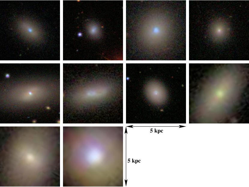
Figure 7.— SDSS images of high-metallicity low-mass galaxies with bright and/or blue cores, scaled to $5\times 5$ kpc, with $M_{B}$ decreasing to the right and down so that the faintest galaxy is in the upper-left corner.

4. Conclusions

We have identified a sample of 41 low-luminosity high–oxygen abundance outliers from the mass–metallicity relation.

1. These galaxies are fairly isolated and none show any signs of morphological disturbance. It is likely, however, that the handful of galaxies in this sample which are possible group or cluster members have disturbed gas morphologies, due to e.g., ram-pressure stripping. However, environmental effects cannot account for the large gas-phase oxygen abundances observed in all of these galaxies.

2. Based on the effective yield considerations of Dalcanton (2007) and various related observational results (Grebel et al., 2003; Dellenbusch et al., 2007; Lee et al., 2006; Boselli et al., 2008), we predict that these galaxies should have low gas fractions relative to other dwarf galaxies of similar stellar masses and star formation rates in similar environments but with more typical (i.e., lower) oxygen abundances. Furthermore, in this scenario, the stellar metallicities should be consistent with that of other dwarfs of similar luminosity, i.e., the stellar metallicities should be lower than the measured gas-phase abundances.

3. These mass–metallicity outliers appear to be “transitional” dwarf galaxies: because they are running out of star-forming fuel, they are nearing the end of their star formation and becoming typical isolated dwarf spheroidals. This conclusion is most sound for the $\mbox{M}_{\star}<9.1M_{\sun}$ galaxies which are observed to have low specific star formation rates. More data—specifically, gas fractions and stellar metallicities—are needed to help elucidate the situation for the higher mass galaxies.

References

- Adelman-McCarthy et al. (2008) Adelman-McCarthy, J. K., Agüeros, M. A., Allam, S. S., Allende Prieto, C., Anderson, K. S. J., Anderson, S. F., Annis, J., Bahcall, N. A., Bailer-Jones, C. A. L., Baldry, I. K., Barentine, J. C., Bassett, B. A., Becker, A. C., Beers, T. C., Bell, E. F., Berlind, A. A., Bernardi, M., Blanton, M. R., Bochanski, J. J., Boroski, W. N., Brinchmann, J., Brinkmann, J., Brunner, R. J., Budavári, T., Carliles, S., Carr, M. A., Castander, F. J., Cinabro, D., Cool, R. J., Covey, K. R., Csabai, I., Cunha, C. E., Davenport, J. R. A., Dilday, B., Doi, M., Eisenstein, D. J., Evans, M. L., Fan, X., Finkbeiner, D. P., Friedman, S. D., Frieman, J. A., Fukugita, M., Gänsicke, B. T., Gates, E., Gillespie, B., Glazebrook, K., Gray, J., Grebel, E. K., Gunn, J. E., Gurbani, V. K., Hall, P. B., Harding, P., Harvanek, M., Hawley, S. L., Hayes, J., Heckman, T. M., Hendry, J. S., Hindsley, R. B., Hirata, C. M., Hogan, C. J., Hogg, D. W., Hyde, J. B., Ichikawa, S.-i., Ivezić, Ž., Jester, S., Johnson, J. A., Jorgensen, A. M., Jurić, M., Kent, S. M., Kessler, R., Kleinman, S. J., Knapp, G. R., Kron, R. G., Krzesinski, J., Kuropatkin, N., Lamb, D. Q., Lampeitl, H., Lebedeva, S., Lee, Y. S., Leger, R. F., Lépine, S., Lima, M., Lin, H., Long, D. C., Loomis, C. P., Loveday, J., Lupton, R. H., Malanushenko, O., Malanushenko, V., Mandelbaum, R., Margon, B., Marriner, J. P., Martínez-Delgado, D., Matsubara, T., McGehee, P. M., McKay, T. A., Meiksin, A., Morrison, H. L., Munn, J. A., Nakajima, R., Neilsen, Jr., E. H., Newberg, H. J., Nichol, R. C., Nicinski, T., Nieto-Santisteban, M., Nitta, A., Okamura, S., Owen, R., Oyaizu, H., Padmanabhan, N., Pan, K., Park, C., Peoples, J. J., Pier, J. R., Pope, A. C., Purger, N., Raddick, M. J., Re Fiorentin, P., Richards, G. T., Richmond, M. W., Riess, A. G., Rix, H.-W., Rockosi, C. M., Sako, M., Schlegel, D. J., Schneider, D. P., Schreiber, M. R., Schwope, A. D., Seljak, U., Sesar, B., Sheldon, E., Shimasaku, K., Sivarani, T., Smith, J. A., Snedden, S. A., Steinmetz, M., Strauss, M. A., SubbaRao, M., Suto, Y., Szalay, A. S., Szapudi, I., Szkody, P., Tegmark, M., Thakar, A. R., Tremonti, C. A., Tucker, D. L., Uomoto, A., Vanden Berk, D. E., Vandenberg, J., Vidrih, S., Vogeley, M. S., Voges, W., Vogt, N. P., Wadadekar, Y., Weinberg, D. H., West, A. A., White, S. D. M., Wilhite, B. C., Yanny, B., Yocum, D. R., York, D. G., Zehavi, I., & Zucker, D. B. 2008, ApJS, 175, 297
- Adelman-McCarthy et al. (2006) Adelman-McCarthy, J. K., Agüeros, M. A., Allam, S. S., Anderson, K. S. J., Anderson, S. F., Annis, J., Bahcall, N. A., Baldry, I. K., Barentine, J. C., Berlind, A., Bernardi, M., Blanton, M. R., Boroski, W. N., Brewington, H. J., Brinchmann, J., Brinkmann, J., Brunner, R. J., Budavári, T., Carey, L. N., Carr, M. A., Castander, F. J., Connolly, A. J., Csabai, I., Czarapata, P. C., Dalcanton, J. J., Doi, M., Dong, F., Eisenstein, D. J., Evans, M. L., Fan, X., Finkbeiner, D. P., Friedman, S. D., Frieman, J. A., Fukugita, M., Gillespie, B., Glazebrook, K., Gray, J., Grebel, E. K., Gunn, J. E., Gurbani, V. K., de Haas, E., Hall, P. B., Harris, F. H., Harvanek, M., Hawley, S. L., Hayes, J., Hendry, J. S., Hennessy, G. S., Hindsley, R. B., Hirata, C. M., Hogan, C. J., Hogg, D. W., Holmgren, D. J., Holtzman, J. A., Ichikawa, S.-i., Ivezić, Ž., Jester, S., Johnston, D. E., Jorgensen, A. M., Jurić, M., Kent, S. M., Kleinman, S. J., Knapp, G. R., Kniazev, A. Y., Kron, R. G., Krzesinski, J., Kuropatkin, N., Lamb, D. Q., Lampeitl, H., Lee, B. C., Leger, R. F., Lin, H., Long, D. C., Loveday, J., Lupton, R. H., Margon, B., Martínez-Delgado, D., Mandelbaum, R., Matsubara, T., McGehee, P. M., McKay, T. A., Meiksin, A., Munn, J. A., Nakajima, R., Nash, T., Neilsen, Jr., E. H., Newberg, H. J., Newman, P. R., Nichol, R. C., Nicinski, T., Nieto-Santisteban, M., Nitta, A., O’Mullane, W., Okamura, S., Owen, R., Padmanabhan, N., Pauls, G., Peoples, J. J., Pier, J. R., Pope, A. C., Pourbaix, D., Quinn, T. R., Richards, G. T., Richmond, M. W., Rockosi, C. M., Schlegel, D. J., Schneider, D. P., Schroeder, J., Scranton, R., Seljak, U., Sheldon, E., Shimasaku, K., Smith, J. A., Smolčić, V., Snedden, S. A., Stoughton, C., Strauss, M. A., SubbaRao, M., Szalay, A. S., Szapudi, I., Szkody, P., Tegmark, M., Thakar, A. R., Tucker, D. L., Uomoto, A., Vanden Berk, D. E., Vandenberg, J., Vogeley, M. S., Voges, W., Vogt, N. P., Walkowicz, L. M., Weinberg, D. H., West, A. A., White, S. D. M., Xu, Y., Yanny, B., Yocum, D. R., York, D. G., Zehavi, I., Zibetti, S., & Zucker, D. B. 2006, ApJS, 162, 38
- Assef et al. (2008) Assef, R. J., Kochanek, C. S., Brodwin, M., Brown, M. J. I., Caldwell, N., Cool, R. J., Eisenhardt, P., Eisenstein, D., Gonzalez, A. H., Jannuzi, B. T., Jones, C., McKenzie, E., Murray, S. S., & Stern, D. 2008, ApJ, 676, 286
- Baldwin et al. (1981) Baldwin, J. A., Phillips, M. M., & Terlevich, R. 1981, PASP, 93, 5
- Boselli et al. (2008) Boselli, A., Boissier, S., Cortese, L., & Gavazzi, G. 2008, ApJ, 674, 742
- Bresolin (2006) Bresolin, F. 2006, astro-ph/0608410
- Bresolin (2007) —. 2007, ApJ, 656, 186
- Brinchmann et al. (2004) Brinchmann, J., Charlot, S., White, S. D. M., Tremonti, C., Kauffmann, G., Heckman, T., & Brinkmann, J. 2004, MNRAS, 351, 1151
- Cid Fernandes et al. (2005) Cid Fernandes, R., Mateus, A., Sodré, L., Stasińska, G., & Gomes, J. M. 2005, MNRAS, 358, 363
- Cooper et al. (2008) Cooper, M. C., Tremonti, C. A., Newman, J. A., & Zabludoff, A. I. 2008, arXiv:0805.0308
- Dalcanton (2007) Dalcanton, J. J. 2007, ApJ, 658, 941
- Delahaye & Pinsonneault (2006) Delahaye, F. & Pinsonneault, M. H. 2006, ApJ, 649, 529
- Dellenbusch et al. (2007) Dellenbusch, K. E., Gallagher, III, J. S., & Knezek, P. M. 2007, ApJ, 655, L29
- Ebeling et al. (1998) Ebeling, H., Edge, A. C., Bohringer, H., Allen, S. W., Crawford, C. S., Fabian, A. C., Voges, W., & Huchra, J. P. 1998, MNRAS, 301, 881
- Ellison et al. (2008) Ellison, S. L., Patton, D. R., Simard, L., & McConnachie, A. W. 2008, ApJ, 672, L107
- Fischera & Dopita (2005) Fischera, J., & Dopita, M. 2005, ApJ, 619, 340
- Finlator & Davé (2008) Finlator, K. & Davé, R. 2008, MNRAS, 385, 2181
- Garnett & Shields (1987) Garnett, D. R. & Shields, G. A. 1987, ApJ, 317, 82
- Grebel et al. (2003) Grebel, E. K., Gallagher, III, J. S., & Harbeck, D. 2003, AJ, 125, 1926
- Gu et al. (2006) Gu, Q., Zhao, Y., Shi, L., Peng, Z., & Luo, X. 2006, AJ, 131, 806
- Karachentsev (2005) Karachentsev, I. D. 2005, AJ, 129, 178
- Kauffmann et al. (2003) Kauffmann, G., Heckman, T. M., White, S. D. M., Charlot, S., Tremonti, C., Brinchmann, J., Bruzual, G., Peng, E. W., Seibert, M., Bernardi, M., Blanton, M., Brinkmann, J., Castander, F., Csábai, I., Fukugita, M., Ivezic, Z., Munn, J. A., Nichol, R. C., Padmanabhan, N., Thakar, A. R., Weinberg, D. H., & York, D. 2003, MNRAS, 341, 33
- Kennicutt (1998) Kennicutt, Jr., R. C. 1998, ApJ, 498, 541
- Kewley & Dopita (2002) Kewley, L. J. & Dopita, M. A. 2002, ApJS, 142, 35
- Kewley & Ellison (2008) Kewley, L. J. & Ellison, S. L. 2008, arXiv:0801.1849
- Kewley et al. (2006) Kewley, L. J., Groves, B., Kauffmann, G., & Heckman, T. 2006, MNRAS, 372, 961
- Köppen et al. (2007) Köppen, J., Weidner, C., & Kroupa, P. 2007, MNRAS, 375, 673
- Larson (1974) Larson, R. B. 1974, MNRAS, 169, 229
- Lee et al. (2006) Lee, H., Skillman, E. D., Cannon, J. M., Jackson, D. C., Gehrz, R. D., Polomski, E. F., & Woodward, C. E. 2006, ApJ, 647, 970
- Lequeux et al. (1979) Lequeux, J., Peimbert, M., Rayo, J. F., Serrano, A., & Torres-Peimbert, S. 1979, A&A, 80, 155
- McGaugh (1991) McGaugh, S. S. 1991, ApJ, 380, 140
- Michel-Dansac et al. (2008) Michel-Dansac, L., Lambas, D. G., Alonso, M. S., & Tissera, P. 2008, arXiv:0802.3904
- Pettini & Pagel (2004) Pettini, M. & Pagel, B. E. J. 2004, MNRAS, 348, L59
- Russell & Dopita (1990) Russell, S. C. & Dopita, M. A. 1990, ApJS, 74, 93
- Tremonti et al. (2004) Tremonti, C. A., Heckman, T. M., Kauffmann, G., Brinchmann, J., Charlot, S., White, S. D. M., Seibert, M., Peng, E. W., Schlegel, D. J., Uomoto, A., Fukugita, M., & Brinkmann, J. 2004, ApJ, 613, 898
- Unterborn & Ryden (2008) Unterborn, C. T. & Ryden, B. S. 2008, arXiv:0801.2400
- Zaritsky et al. (1994) Zaritsky, D., Kennicutt, Jr., R. C., & Huchra, J. P. 1994, ApJ, 420, 87