Landau-Zener transitions in a semiconductor quantum dot

Abstract

We study the transitions between neighboring energy levels in a quasi-one-dimensional semiconductor quantum dot with two interacting electrons in it, when it is subject to a linearly time-dependent electric field. We analyze the applicability of simple two-level Landau-Zener model to describe the evolution of the probability amplitudes in this realistic system. We show that the Landau-Zener model works very well when it is viewed in the adibatic basis, but it is not as robust in the diabatic basis.

I Introduction

The Landau-Zener (LZ) model describes in a simplified way the ubiquitous situation of avoided crossings of energy levels in quantum mechanics zen . This happens in numerous areas of physics such as quantum optics, atomic physics, nuclear physics, etc. In spite of its simplified nature, the LZ model often captures the essential features of avoided level crossings in realistic systems and the list of its applications continues to grow.

Recently, we have proposed a generic quantum control method based on the navigation of the energy spectrum. The navigation of the spectrum is done varying a control parameter diabatically and adiabatically. The possibility of traveling through a complex spectrum depends crucially on the nature of the energy level crossings. Our method requires that the system behave locally (at avoided crossings) like a LZ model, in the sense that complete diabatic and adiabatic transitions be possible. So, the first step in the application of this method to a realistic system must be a careful examination of the validity of this condition. Note that in a realistic system the interaction between levels is often intricate and the possibility that the LZ model worked has been discussed bul-dod-kus ; san-ver-wis . Recently, we successfully applied this control strategy to a quantum dot system and the isomerization of a LiCN molecule. In the present paper we analyse in detail the issue of the applicability of the LZ model to the avoided crossings of the two-electron quantum-dot system studied in Refs. mur-wis-tam ; wis-mur-tam .

Quantum dots are prime candidates to study the ideas and proposals of quantum control, given their flexible and tunable properties. In this paper, we continue the study of a quasi-one-dimensional double-dot system with two interacting electrons. Because of the one-dimensionality, this system is well suited to investigate new methods of quantum control, and at the same time it incorporates the important aspect of the interparticle interaction treated exactly. We remark that the presence of interactions between particles is crucial in the new science of quantum information processing.

The article is organized as follows: In order to make the work as self-contained as possible, in the next section we review the well-known Landau-Zener Model. In Section III we describe our system and in the following section we present the results concerning the applicability of the LZ model. We conclude with some final remarks.

II Landau-Zener Model

The LZ model zen attempts to describe the universal situation of two levels interacting at an avoided crossing when a parameter $\lambda$ in the Hamiltonian is varied. The model consists of a two-level system described by a parameter-dependent Hamiltonian, which expressed in the diabatic basis reads

$$H=\left[\begin{array}[]{cc}\varepsilon_{1}(\lambda)&\delta\\ \delta&\varepsilon_{2}(\lambda)\end{array}\right],$$ (1)

where $\delta$ is a constant while $\varepsilon_{1}$ and $\varepsilon_{2}$ are linear functions of $\lambda$: $\varepsilon_{1}=\overline{\varepsilon}+\alpha_{1}(\lambda-\overline{\lambda})$, $\varepsilon_{2}=\overline{\varepsilon}+\alpha_{2}(\lambda-\overline{\lambda})$. The center of the avoided crossing is located at $\overline{\lambda}$ and $\overline{\varepsilon}$ [see Fig. 1]. The diabatic basis, $|1\rangle$ and $|2\rangle$, are parameter-independent eigenstates of the Hamiltonian Eq. (1) with $\delta=0$.

The eigenenergies $E_{1}(\lambda)$ and $E_{2}(\lambda)$ of the Hamiltonian (1) are two hyperbolas (the adiabatic curves) as shown in Fig. 1. The eigenstates associated to those energies are the so-called adiabatic states, which we denote $|\phi_{1}(\lambda)\rangle$ and $|\phi_{2}(\lambda)\rangle$. The asymptotes to the energy hyperbolas are the diabatic straight lines $\varepsilon_{1}(\lambda)$ and $\varepsilon_{2}(\lambda)$. The shortest distance between the hyperbolas is $2\delta$.

In his seminal paper, Zener considered the parameter $\lambda$ as a linear function of time and obtained the asymptotic probabilities of transitions between the diabatic states in this time-dependent problem. Assuming that the state $|1\rangle$ is the initial state (at $t\rightarrow-\infty$) and $\lambda(t)=\beta\,t$, and calling $|\psi(t)\rangle$ the evolving wave function, the asymptotic probability to end up in the other diabatic state is

$$P_{2}(t\rightarrow\infty) = |\langle 2|\psi(t\rightarrow\infty)\rangle|^{2}=1-\exp{\left[\frac{-2\pi\delta^{2}}{\hbar|\dot{\varepsilon}_{1}-\dot{\varepsilon}_{2}|}\right]}$$ (2)

$$= 1-\exp{\left[\frac{-2\pi\delta^{2}}{\hbar\beta|\alpha_{1}-\alpha_{2}|}\right]}.$$

Figure 1: Schematic plot of an avoided crossing. The solid lines represent the adiabatic levels $E_{1}(\lambda)$ and $E_{2}(\lambda)$. The asymptotes to the energy hyperbolas are the diabatic straight lines $\varepsilon_{1}(\lambda)$ and $\varepsilon_{2}(\lambda)$ (dashed lines). The center of the avoided crossing at $\overline{\lambda}$ and $\overline{\varepsilon}$ is inidicated with dotted lines.

The two limiting cases in terms of $\beta$ (the rate of change of the parameter $\lambda$) are:
i) Slow transition: $\beta\ll\frac{2\pi\delta^{2}}{\hbar|\alpha_{1}-\alpha_{2}|}$. In this case the system follows the adiabatic curve going from the initial diabatic state to the other one.
ii) Rapid transition: $\beta\gg\frac{2\pi\delta^{2}}{\hbar|\alpha_{1}-\alpha_{2}|}$. The evolution takes place on the diabatic curve and the system remains in the initial diabatic state.
These limiting cases play a central role in our control method mur-wis-tam , as they give us quantitative criteria to choose either the diabatic or adiabatic paths in traversing an avoided crossing wis-mur-tam .

More recently, the complete time dependence of the occupation probabilities in both the diabatic ($|\langle 1|\psi(t)\rangle|^{2}$, $|\langle 2|\psi(t)\rangle|^{2}$) and adiabatic basis ($|\langle\phi_{1}(\lambda)|\psi(t)\rangle|^{2},|\langle\phi_{2}(\lambda)|\psi(t)\rangle|^{2}$) sets has been obtained vit ; dam-zur .

III The system: Quasi-one-dimensional doble quantum dot with two interacting electrons

Let us consider a quasi-one-dimensional double quantum dot with two interacting electrons in the presence of a uniform longitudinal electric field. This system is interesting for two reasons. First, this type of system is experimentally realizable nowadays, and second, the nonperturbative interparticle interaction is taken into account.

We have chosen a semiconductor system with realistic dimensions: it is an elongated quantum dot $100\,\mbox{nm}$ long and $50\,\mbox{\AA}$ wide. Due to the small thickness of the structure, the energies of the transverse modes are widely spaced and it is enough to consider only the lowest transverse state. Therefore, an effective Hamiltonian that depends only on the longitudinal coordinate $z$ describes the dynamics of the system tam-met

$$H \equiv -\frac{\hbar^{2}}{2m}(\frac{\partial^{2}}{\partial z_{1}^{2}}+\frac{\partial^{2}}{\partial z_{2}^{2}})+V(z_{1})+V(z_{2})$$ (3)

$$+V_{C}(|z_{1}-z_{2}|)-e(z_{1}+z_{2})E(t)\,,$$

where $m$ is the electron effective mass in the semiconductor material, $V_{C}$ is the Coulomb interaction between the electrons, $V$ is the confining potential, and $E(t)$ is a time-dependent external electric field. There is no restriction regarding the choice of the confining potential in the $z$-direction, but we have selected the double-well configuration shown in Fig. 2. Double-well potentials are interesting due to the interplay between tunneling and localization. Moreover, in our two-electron system these important phenomena can be related to the Coulomb interaction. In all of the time evolutions that we will analyze, we assume that the wave function is initially a singlet (antisymmetric spin wave function). Since the Hamiltonian is spin independent, the spin wave function remains a singlet and the orbital part of the wave function is symmetric at all times.

Figure 2: Confining double well potential in the longitudinal direction of the coupled quantum dot structure. The external electric field is $E=0$ (solid lines) and $E=12\,\mbox{kV/cm}$ (dashed lines).

We have used the time-dependent electric field $E(t)$ as the control parameter mur-wis-tam ; wis-mur-tam . The first step is to understand the behavior of our system when the electric field is taken as a constant. So, we have computed numerically the eigenergies and eigenfunctions of the system as a function of a constant electric field. We numerically diagonalize the Hamiltonian of Eq. (3) expanded in the basis set of Slater determinants constructed with the 12 bound single-particle states of the double-well potential. The two-particle basis set has then 12*(12+1)/2=78 states.

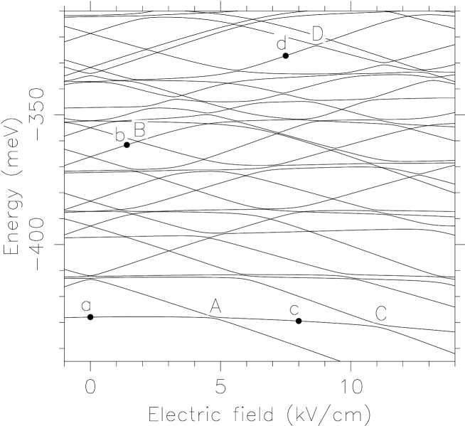
Figure 3: The energy spectrum of the two interacting electrons confined in a quasi-one-dimensional double-well semiconductor nanostructure as a function of an external uniform electric field. It is plotted the first 31 energy levels. See text for details.

The energy spectrum as a function of the external electric field is shown in Fig. 3. We can see that the spectrum is composed by fairly straight lines which never cross each other, resulting in frequent avoided crossings. For the low-lying states included in our spectrum, and far from the avoided crossings, the adiabatic states have clear localization properties connected with their slope (see Fig. 2 in Ref. mur-wis-tam ):
i) in the eigenstates corresponding to negative slope both electrons are in the left well,
ii) the states associated to the positive slope are localized on the right well, and
iii) the states with neutral slope have one electron in each well.
At avoided crossings, the eigenstates mix their localization characteristics reaching the maximal degree of mixing at the center of the avoided crossing.

IV Analysis of the applicability of the Landau-Zener model

In our previous works we introduced a method of quantum control via traveling in the energy spectrum of a quantum system mur-wis-tam ; wis-mur-tam . The building blocks of this method are, on the one hand, the adiabatic evolutions far from avoided crossings, and on the other, the slow and fast evolutions employed at avoided crossings in order to shift in a controlled way from one adiabatic path to a neighboring one. If the system behaves locally like a LZ this possibility will be guaranteed. For this reason, in this section we will analyze the range of validity or applicability of the Landau-Zener model to describe the transitions at the avoided crossings of our system.

We begin by studying the avoided crossing labelled “A” in Fig. 3, between the ground state and the first excited state near the value of the electric field $E=5\,\mbox{kV/cm}$. Initially the system is in the ground state with no electric field (state labelled “a” in Fig. 3) and we study the probability to remain in the ground state when the electric field is increased linearly with time at different velocities. This corresponds to the adiabatic probability $|\langle\phi_{1}(E)|\psi(t)\rangle|^{2}$ introduced at the end of Section II. These probabilities are shown in Fig. 4. We remark that in order to compare the results for different velocities, we plot in Fig. 4 the probabilities as functions of the electric field rather than as functions of time. In Fig. 4 we present the adiabatic probability for the following velocities, $\dot{E}=0.07,0.27,0.53,1.07,4.27\,\mbox{kV/cm ps}$.

We now compute the adiabatic probabilities in the LZ model. The first step is to fit the parameters $\delta$, the location of the avoided crossing, $\alpha_{1}$, and $\alpha_{2}$ footnote of the two-level Hamiltonian of Eq. (1) to the avoided crossing under study. As initial state we take the adiabatic LZ state for the value of $\lambda$ that corresponds to state “a” in Fig. 3. We compute the adiabatic probabilities in the LZ model for the previous set of rates of change of the electric field. These results are plotted with solid lines in Fig. 4. We can see that our system is well described by the LZ model for the whole range of velocities considered. Moreover, we see that the asymptotic probability obtained by Zener (horizontal dashed lines in Fig. 4) gives accurate results far from the avoided crossing. Note that far from the avoided crossing the diabatic and adiabatic states in the LZ model are essentially the same.

Figure 4: Adiabatic transition probabilities $|\langle\phi_{1}(E)|\psi(t)\rangle|^{2}$ at the lowest avoided crossing (labelled “A” in Fig. 3) for various rates of change of the control parameter. The velocities are: $\dot{E}=0.07(\triangle),0.27(\Box),0.53(\times),1.07(\circ),4.27\,(*)\,\mbox{kV/cm ps}$. The initial state in the exact evolution is the one labelled “a” in Fig. 3. The solid lines give the adiabatic probabilities in the LZ model and the dotted lines are the asymptotic LZ probabilities given in Eq. (2).

We have done similar analyses for other avoided crossings of the energy spectrum. Namely, we start with the states labelled “b”, “c”, and “d” in Fig. 3, and we study the transition probabilities in the adjacent avoided crossings “B”, “C”, and “D”, respectively. In Fig. 5 we show the results, which verify the previous conclusion, in the sense that in the adiabatic basis the two-level LZ model fits very well the exact results. It is worth noting here that in our previous work of Ref. mur-wis-tam ; wis-mur-tam we travel in the spectrum (that is, we attempt to go from a given adiabatic state to another one). In this sense, the above given results are the most relevant ones to judge the applicability of our control method.

Figure 5: Adiabatic transition probabilities at various avoided crossings (labeled ”B”, ”C” and ”D” in Fig. 3). The initial states in these evolutions are labelled in Fig. 3 as ”b” [panel (a)] , ”c” [panel (b)], and ”d” [panel (c)] . The velocities are: (a) $\dot{E}=0.0015(\triangle),0.0077(\Box),0.015(\times),0.07(\circ),4.27\,(*)\,\mbox{kV/cm ps}$, (b) $\dot{E}=0.07\,(\triangle),0.53\,(\Box),1.27\,(\times),4.27\,(\circ),40.0\,(*)\,\mbox{kV/cm ps}$, and (c) $\dot{E}=0.003\,(\triangle),0.07\,(\Box),0.27\,(\times),0.53\,(\circ),4.27\,(*)\,\mbox{kV/cm ps}$,

Since the LZ model is defined on the basis of diabatic states, it is perhaps more natural to perform the former analysis on that basis set. However, the question arises of what the diabatic states are in our realistic system. Indeed, in a multilevel system like ours the two states involved in the avoided crossing become mixed with other states and therefore acquire a dependence on the control parameter (which is not allowed for in the usual LZ model). It is thus an interesting question to ask whether it is possible to find a “fixed” basis set which could play the role of the diabatic basis in the LZ model. For example, we now calculate the probability $|\langle\phi_{1}(E_{0})|\psi(t)\rangle|^{2}$, where $|\phi_{1}(E_{0})\rangle$ is the the initial state in the dynamic passage of an avoided crossing. That is, we are considering $|\phi_{1}(E_{0})\rangle$ as being one of the diabatic basis states. We now do this for the lowest crossing taking $E_{0}=0$, and compare with the results of using the two-level LZ model in Fig. 6. One can clearly see that the agreement between the two calculations is not very good. This can be understood with the help of the inset of Fig. 6, which shows the overlaps $|\langle\phi_{1}(E=0)|\phi_{1}(E)\rangle|^{2}$ and $|\langle\phi_{1}(E=0)|\phi_{2}(E)\rangle|^{2}$ as functions of the electric field $E$. It is clear from the inset, especially from $|\langle\phi_{1}(E=0)|\phi_{2}(E)\rangle|^{2}$ (dashed line), that the hypothesis of a parameter-independent diabatic state is not satisfied (that the overlap is not equal to one far from the avoided crossing), and therefore the LZ model tends to fail. However, in other avoided crossings we have observed that it is possible to find good diabatic states (which are fairly parameter-independent around the avoided crossing). For example, we repeated the previous analysis for the avoided crossing labelled “B” in Fig. 3, choosing $|\phi_{16}(E=1.4\,\mbox{kV/cm})\rangle$ as one of the diabatic states. In Fig. 7, we plot the probability $|\langle\phi_{16}(E=1.4\,\mbox{kV/cm})|\psi(t)\rangle|^{2}$, which shows a better agreement than the one in Fig.  6. We remark that, as can be seen in the inset of Fig. 7, the state $|\phi_{16}(E=1.4\,\mbox{kV/cm})\rangle$ is a good choice of diabatic state, since the overlap $|\langle\phi_{16}(E=1.4\,\mbox{kV/cm})|\phi_{17}(E)\rangle|^{2}$ is close to one at the right of the crossing and close to zero to the left (see dashed line). The behavior seen in the inset is exactly what one obtains in the LZ model for the overlaps between the diabatic and adiabatic bases.

Figure 6: Diabatic transition probabilities $|\langle\phi_{1}(E_{0}=0)|\psi(t)\rangle|^{2}$ (dotted lines) at the lowest avoided crossing, labelled “A” in Fig. 3. The rates of change of the control parameter, the electric field $E$, are the same as Fig. 4. In solid lines, the corresponding probabilities in the LZ model. Inset: overlaps $|\langle\phi_{1}(E=0)|\phi_{1}(E)\rangle|^{2}$ (solid line) and $|\langle\phi_{1}(E=0)|\phi_{2}(E)\rangle|^{2}$ (dashed line).

Figure 7: Diabatic transition probabilities $|\langle\phi_{16}(E=1.4\,\mbox{kV/cm)}|\psi(t)\rangle|^{2}$ (dotted lines) at the avoided crossing, labelled “B” in Fig. 3. The rates of change of the control parameter, the electric field $E$, are the same as in Fig.  5(a). In solid lines, the corresponding probabilities in the LZ model. Inset: overlaps $|\langle\phi_{16}(E=1.4\,\mbox{kV/cm})|\phi_{16}(E)\rangle|^{2}$ (solid line) and $|\langle\phi_{16}(E=1.4\,\mbox{kV/cm})|\phi_{17}(E)\rangle|^{2}$ (dashed line).

V Final Remarks

We have studied the applicability of the LZ model in a realistic system: a quasi-one-dimensional double quantum dot with two interacting electrons. We showed that the LZ model works very well when it is viewed in the adiabatic basis. This result is the cornerstone for the quantum controlability using the method of control introduced in mur-wis-tam .

However, when seen in the diabatic basis the results are not so robust as in the case of the adiabatic basis. This is due to the fact that, for multilevel systems, a proper diabatic basis does not exist. Rather, the pair of interacting levels at an avoided crossing become mixed with other states and acquire a dependence with the control parameter even far from the avoided crossings.

References

- (1) C. Zener, Proc. R. Soc. London, Ser. A 137, 696 (1932).
- (2) A. Bulgac, G. Do Dang, and D. Kusnezov, Ann. Phys. (Leipzig) 242, 1 (1995); Phys. Rep. 264, 67 (1996).
- (3) M. J. Sánchez, E. Vergini, and D. A. Wisniacki, Phys. Rev. E 54, 4812 (1996).
- (4) G. E. Murgida, D. A. Wisniacki, and P. I. Tamborenea, Phys. Rev. Lett. 99, 036806 (2007).
- (5) D. A. Wisniacki, G. E. Murgida, and P. I. Tamborenea, AIP Proc. 963, 840 (2007).
- (6) N. V. Vitanov, Phys. Rev. A 59, 988 (1999).
- (7) B. Damski and W. H. Zurek, Phys. Rev. A 73, 063405 (2006).
- (8) P. I. Tamborenea and H. Metiu, Phys. Rev. Lett. 83, 3912 (1999).
- (9) Actually only the difference enters in the evolution of the two-level LZ system. The location of the avoided crossing is irrelevant in terms of the probabilities, but is is necessary to compare the results of the two calculations.