Confinement Effects on Phase Behavior of Soft Matter Systems

When systems that can undergo phase separation between two coexisting phases in the bulk are confined in thin film geometry between parallel walls, the phase behavior can be profoundly modified. These phenomena shall be described and exemplified by computer simulations of the Asakura-Oosawa model for colloid-polymer mixtures, but applications to other soft matter systems (e.g. confined polymer blends) will also be mentioned. Typically a wall will prefer one of the phases, and hence the composition of the system in the direction perpendicular to the walls will not be homogeneous. If both walls are of the same kind, this effect leads to a distortion of the phase diagram of the system in thin film geometry, in comparison with the bulk, analogous to the phenomenon of “capillary condensation” of simple fluids in thin capillaries. In the case of “competing walls”, where both walls prefer different phases of the two phases coexisting in the bulk, a state with an interface parallel to the walls gets stabilized. The transition from the disordered phase to this “soft mode phase” is rounded by the finite thickness of the film and not a sharp phase transition. However, a sharp transition can occur where this interface gets localized at (one of) the walls. The relation of this interface localization transition to wetting phenomena is discussed. Finally, an outlook to related phenomena is given, such as the effects of confinement in cylindrical pores on the phase behavior, and more complicated ordering phenomena (lamellar mesophases of block copolymers or nematic phases of liquid crystals under confinement).

1 Introduction

The current interest in the construction of nanoscopic devices [1, 2, 3, 4, 5] demands a better understanding of the phase behavior of fluids confined in pores or slits of nanoscopic linear dimensions [6, 7, 8, 9, 10, 11, 12]. Knowledge on the phase behavior of confined fluids is a prerequisite to understand their dynamics [13, 14, 15], as well as for the analysis of flow through very thin capillaries [16, 17], nanoscale capillary imbibition [18, 19], and related microfluidic or nanofluidic devices.

Obviously, an interplay must be expected between surface effects on the fluid due to the confining walls, such as adsorption [20, 21, 22, 23], formation of wetting (or drying) layers [24, 25, 26, 27], and finite size effects [28, 29, 30] due to the finite width of the capillary. However, understanding the nanoscopic confinement of real fluids consisting of small molecules is very difficult due to additional effects, resulting from the lateral variation of the wall potential caused by wall roughness or even the atomistic corrugation [31, 32] of the wall.

While there has been an enormous activity to study theoretically and by computer simulation confinement effects on simple fluid models such as the Ising lattice gas model [11] or simple Lennard-Jones systems [10, 12] and rich predictions from phenomenological theories are available as well [7, 8, 9, 10, 11, 12, 33, 34, 35, 36, 37, 38, 39], it is difficult to find pertinent experiments to which such work could be compared. However, it is much more promising to study confinement effects on soft matter systems: due to the mesoscopic length scales of the particles that one encounters when one studies mixtures of polymers and colloids [40] or polymer blends [41, 42], effects due to the atomistic corrugation of the walls are much less important; also the large size of colloidal particles enables more detailed experimental observations; e.g. individual particles can be tracked though real space in real time using confocal microscopy [43] and interface fluctuations in mixtures of colloids and polymers can be directly observed [44, 45]. Moreover, colloids are model systems for the study of phase behavior, since by changing suitable parameters the strength and range of effective interactions can be varied over a wide range [46, 47, 48]. Also the interaction of colloidal particles with the confining walls can be tuned, e.g. by coating the wall with a polymer brush [49, 50, 51, 52] and controlling the polymer-wall interaction via variation of the grafting density and/or chain length of the anchoring flexible polymer [52, 53]. In particular, for colloid-polymer mixtures both the radius of the (spherical) colloidal particles and the size ratio between colloids and polymer coils controls the location of the critical point where the phase separation in a colloid-rich and a polymer-rich phase sets in [40].

Similarly, also blends of long flexible polymers are a very suitable model system to study the effect of confinement in a thin film geometry on phase separation experimentally as well [41, 42, 54]. Again, already the location of the critical temperature of phase separation in the bulk can be varied over a wide range, by suitable choices of the polymeric species, and their chain lengths [55, 56, 57]. In addition, characteristic lengths of the problem such as the correlation length of composition fluctuations [57], the (intrinsic) interfacial width between coexisting phases [57], etc., are much larger than interatomic distances, and hence also for these systems experimental probes are available which would lack sensitivity for small molecule systems. E.g., for the study of the anomalous broadening of interfaces depending on the film thickness [41, 42], which is one of the characteristic signatures of the “soft mode phase” [36, 37] in a system with “competing walls” [38], a nuclear-reaction based depth profiling method [54] was used. This method can resolve the very wide interfaces in such soft matter systems, while it would be unsuitable for the much narrower interfaces in mixtures of small molecules.

As is evident from this introductory discussion, and the extensive literature that has already been quoted, the subject is extremely rich, and comprehensive coverage could fill a whole book. Therefore the scope of the present review necessarily must be more narrow. We shall focus in this review almost exclusively on confinement effects of colloid-polymer mixtures [58, 59, 60, 61, 62, 63]. Only spherical colloidal particles shall be discussed, although related phenomena can be studied also for mixtures of polymers with rod-like colloids [64]. Although extensive work has been done for models of polymer blends, both using the self-consistent field theory [65, 66, 67] and simulations [65, 68, 69, 70], we shall not consider this work here, but draw attention to recent reviews [71, 72]. Also, we shall not attempt to review the theory of wetting phenomena [24, 25, 26, 27] and scaling theories of capillary condensation [11, 33] and interface localization transitions [36, 37, 38, 70] but rather refer the reader to another thorough review [11].

In Sec. 2, we shall briefly recall work on phase behavior of the model of Asakura and Oosawa (AO) [73] and Vrij [74], where colloids simply are described as hard spheres which may neither overlap with each other nor overlap with polymers, while the latter may overlap with each other with no energy cost, in the bulk [75, 76, 77, 78, 79, 80, 81, 82, 83]. In Sec. 3 we shall discuss the phase behavior of this AO model when it is confined [58, 59, 60, 61, 62] between symmetrical walls a distance $D$ apart, paying attention to the shift of the critical point as a function of film thickness $D$, and to the change of the critical behavior. Sec. 4 then describes the behavior encountered for asymmetric walls [63], where it is also shown that by variation of the conditions at the walls one can gradually crossover from this interface localization transition to a transition which is of capillary condensation type. Sec. 5 then presents a summary of the results reviewed here, and gives an outlook on related findings in other systems, as well as to more complicated phenomena where the order parameter characterizing the transition is not a simple scalar quantity (as it is for gas-liquid or liquid-liquid type phase separation).

2 Liquid-liquid demixing for the Asakura-Oosawa (AO) model in the bulk

In the AO model [73, 74] colloids are described as hard spheres of radius $R_{\rm c}$, and hence the potential between two colloidal particles at distance $r$ from each other is

$$U_{\rm cc}(r)=\infty\;(r<2R_{\rm c}),\ U_{\rm cc}(r)=0\;({\rm else})\quad.$$ (1)

Similarly, polymers are described as soft spheres of radius $R_{\rm p}$. Remembering that long polymer chains with $N$ subunits have a radius $R_{\rm p}\propto N^{\nu}$ with $\nu\approx 0.59$ in good solvent conditions [56] or $R_{\rm p}\propto N^{1/2}$ in Theta solvents [56], the density $\rho_{\rm p}=N/R^{3}_{p}$ of monomers of a chain inside its own volume is very small, and hence polymer coils can interpenetrate each other with a free energy cost of a few $k_{B}T$ (with $k_{B}$ the Boltzmann constant and $T$ the temperature) [84]. In the AO model, this free energy cost is neglected, and the polymers are treated like particles in an ideal gas, $U_{\rm pp}(r)=0$ irrespective of distance. But, of course, polymers cannot penetrate into the colloidal particles, and hence

$$U_{\rm pc}(r)=\infty\;(r<R_{\rm c}+R_{\rm p}),\,\,U_{\rm pc}(r)=0\;({\rm else}).$$ (2)

As is well-known [40], the polymers cause an (entropic) depletion attraction between the colloidal particles, and as a result, an entropy-driven phase separation occurs, if the volume fractions $\eta_{\rm c}$, $\eta_{\rm p}$ of colloids and polymers are sufficiently high (Fig. 1). Here $\eta_{\rm c}$, $\eta_{\rm p}$ are defined in terms of the volume $V$ of the system and the numbers of colloids and polymer, $N_{\rm c}$ and $N_{\rm p}$, respectively, by

$$\eta_{\rm c}=\frac{4\pi}{3}R^{3}_{\rm c}N_{\rm c}/V\quad,\quad n_{p}=\frac{4\pi}{3}R^{3}_{\rm p}N_{\rm p}/V\,,$$ (3)

and $R_{\rm c}=1$ will henceforth be chosen as unit of length. Since both $\eta_{\rm c}$, $\eta_{\rm p}$ are densities of extensive thermodynamic variables, it is useful to carry out a Legendre transform to an intensive thermodynamic variable, where the chemical potential $\mu_{\rm p}$ of the polymers [or their fugacity $z_{\rm p}=\exp(\mu_{\rm p}/k_{B}T)$] is used. It is customary to use instead of $\mu_{\rm p}$ or $z_{\rm p}$ the so-called “polymer reservoir packing fraction” $\eta^{\rm r}_{\rm p}$,

$$\eta^{\rm r}_{\rm p}=z_{\rm p}\Big{(}\frac{4\pi}{3}\Big{)}R^{3}_{\rm p}\,\;$$ (4)

Eq. (4) would be just the volume fraction of polymers in the absence of any colloids, since such a system simply is an ideal gas of polymers.

It is clear that the model defined by Eqs. (1), (2) is a drastic simplification of reality, but in qualitative respects it is remarkably accurate [40]. While various more realistic extensions of the AO model have been considered [79, 84, 85, 86, 87, 88, 89, 90, 91, 92], and sometimes better agreement with experiments [44, 93] is obtained, we disregard such extensions here because in practice there are many additional effects (such as charges on the colloidal particles [94, 95], adsorption of polymers on the colloids [96], etc.) that make a quantitative comparison with experiment elusive.

In early simulation work on the AO model [77, 78] a wider range of volume fractions $\eta_{\rm c}$, $n_{\rm p}$ (and a much wider range of $\eta^{\rm r}_{\rm p}$) was studied, but only a much more limited accuracy than shown in Fig. 1 was obtained. On the basis of this work [77, 78], it was concluded that the agreement between simulations and the mean-field theory of Lekkerkerker et al. [75] is excellent. Fig. 1 demonstrates, however, that the relative deviation between the actual value for $\eta^{\rm r}_{\rm p}$ at the critical point, $\eta^{\rm r}_{\rm p,cr}=0.766\pm 0.002$, deviates from its mean-field prediction [75] by about 30%. This deviation, in fact, is relatively larger than corresponding deviations between mean field theory and accurate simulation results for lattice gas models [97], Lennard-Jones fluids [98], etc. In retrospect, this large deviation between mean-field theory [75] and accurate simulation results for colloid-polymer mixtures [80, 81, 82] is not surprising, since on the length scale of a colloidal particle the depletion attraction has a very short range, and the large absolute size of colloidal particles in this context is not relevant: it would be wrong to infer that colloids should behave mean-field like.

Being interested in the changes in phase behavior due to confinement between walls that are a distance $D\gg R_{\rm c}(=1)$ apart, relatively small changes must be expected, of course. For an analysis of these changes, and in particular for a study how bulk behavior in the limit $D\rightarrow\infty$ is approached, a very good accuracy of the simulation data is absolutely crucial. Thus, it is worthwhile to briefly recall how results such as those shown in Fig. 1 can be obtained, since the methods for the study of the confined systems [61, 62, 63] are closely related to those used in the bulk [80, 81, 82].

We start this recollection by emphasizing that for studying liquid-vapor type phase equilibria the grand-canonical $(\mu VT)$ ensemble of statistical mechanics is the best choice [98], since it avoids problems due to slow relaxation of liquid-vapor interfaces that hamper the use of the canonical ensemble [99, 100]. Also near the critical point the problem of critical slowing down [101] is somewhat less severe in the grand-canonical ensemble [98, 99, 100], and the inevitable finite size effects are relatively easy to handle by finite size scaling methods [28, 29, 30, 102, 103], unlike the popular Gibbs ensemble [104, 105]. So the task of the simulation is to vary the chemical potential $\mu$ of the colloids at fixed $\eta^{\rm r}_{\rm p}$ (as the phase diagram, Fig. 1, suggests, $\eta^{\rm r}_{\rm p}$ is analogous to inverse temperature for ordinary vapor-liquid type transitions [98], where vapor-liquid phase separation is driven by enthalpic rather than entropic forces. Of course, in thermal equilibrium the average colloid fraction $\langle\eta_{\rm c}\rangle$, which is the variable thermodynamically conjugate to $\mu$ (apart from a normalization factor, see Eq. 3), increases monotonously with $\mu$ even when the two-phase coexistence region is crossed, and in the $\langle\eta_{\rm c}\rangle$ vs. $\mu$ curve hence no singularity shows up for any finite linear dimension $L$: only in the thermodynamic limit (where $L\rightarrow\infty$) this “isotherm” develops at $\mu=\mu_{\rm coex}$ a perpendicular part, where $\langle\eta_{\rm c}\rangle$ jumps discontinuously from $\eta_{\rm c}^{\rm V}$ (vapor) to $\eta^{\rm L}_{\rm c}$ (liquid). However, nevertheless phase coexistence is easily recognizable also in a finite volume simulation, when the colloid volume fraction distribution $P(\eta_{\rm c})$ is sampled [98, 99, 100]. In the regime $\eta^{\rm V}_{\rm c}\leq\langle\eta\rangle\leq\eta^{\rm L}_{\rm c}$, $P(\eta_{\rm c})$ has a double peak structure, and for $\mu=\mu_{\rm coex}$ both peaks have equal weight (“equal area rule” [106, 107]).

In order to carry out this program, two obstacles need to be overcome: (i) in order to sample the relative weights of the two peaks of $P(\eta_{\rm c})$, the peak near $\eta^{\rm V}_{\rm c}$ representing the vapor-like phase of the colloid-polymer mixture and the peak near $\eta^{\rm L}_{\rm c}$, the liquid-like phase, the system needs to cross many times a region of very low probability near $\eta_{\rm d}=(\eta^{\rm V}_{\rm c}+\eta^{\rm L}_{\rm c})/2$. This problem, however, can be very efficiently solved by successive umbrella sampling [108]. Fig. 2 shows, as a typical example, distributions $P(\eta_{\rm c})$ that span almost 30 decades. (ii) The second obstacle is the fact that the polymer volume fraction, in the polymer-rich phase, can be very high (exceeding unity, since the polymers are allowed to overlap with no energy cost). Insertion of a colloid particle at a randomly chosen position, which is one of the Monte Carlo (MC) moves that one needs to carry out in grand-canonical Monte Carlo simulations, almost always will be rejected: so a naive implementation of a grand-canonical MC simulation for unfavorable parameters is bound to fail utterly. However, this problem also could be overcome, by the invention of a composite MC move, where in a spherical region with some properly chosen radius $r_{\rm c}$ a randomly selected chosen number $n_{\rm r}$ of polymers is taken out and only then insertion of a colloid is attempted (the reverse move also exists and is constructed such that the detailed balance principle [99, 100] is fulfilled) [81, 82].

We now return to the observation of Fig. 2, that a high free energy barrier $\Delta F$ (choosing units where $k_{B}T=1$) exists, which is independent of $\eta_{\rm c}$ in a broad regime of $\eta_{\rm c}$ around the composition of the rectilinear diameter $\eta_{\rm d}$. The interpretation of this fact is that the system in this region is in a state with two domains, separated by two domain walls, oriented perpendicular to the $z$-direction, and connected into itself by the periodic boundary conditions. This is also confirmed by direct inspection of the configurations of the system. Hence [109]

$$\Delta F=2L^{2}\gamma_{\rm LV},\quad L\rightarrow\infty\,,$$ (5)

where $\gamma_{\rm LV}$ is the interfacial tension between liquid- and gas-like phases, and $L^{2}$ the interfacial area. Thus, estimating $\Delta F$ for a series of cross-sectional areas $L^{2}$ of the simulation box and extrapolating the result for $\gamma_{\rm LV}$ to the thermodynamic limit has become a standard method for the MC estimation of interfacial free energies [99, 100]. Fig. 3 shows typical results for the reduced interfacial tension plotted vs. the order parameter $\eta^{\rm L}_{\rm c}-\eta^{\rm V}_{\rm c}$ and compares them to density functional theory predictions [110]. These simulation results for $\gamma_{\rm LV}$ are also consistent with a capillary wave analysis [83]. Note that the coexistence densities $\eta^{\rm V}_{\rm c}$, $\eta^{\rm L}_{\rm c}$ do approach the predictions from mean field theory rather fast (Fig. 1), for $\eta^{\rm r}_{\rm p}\geq 1.0$ the differences are practically invisible, however, no such convergence is seen for the interfacial tension (Fig. 3). The reason for the strong discrepancies in Fig. 3 is not clear.

We now comment on the treatment of finite size effects. If one naively would take the values of $\eta_{\rm c}$ where $P(\eta_{\rm c)}$ has its two peaks as estimates for $\eta^{\rm V}_{\rm c}$ and $\eta^{\rm L}_{\rm c}$ also in the critical region, one obtains results as shown in Fig. 4: For $\eta_{\rm p}^{\rm r}\geq 0.79$ these estimates are independent of the linear dimension of the simulation box, but for $\eta^{\rm r}_{\rm p}<0.79$ systematic finite size effects appear. E.g., for $\eta^{\rm r}_{\rm p}=0.76$ the difference $\eta^{\rm L}_{\rm c}-\eta^{\rm V}_{\rm c}$ decreases systematically with increasing $L$. While for $\eta^{\rm r}_{\rm p}>\eta^{\rm r}_{\rm p,cr}$ this difference for $L\rightarrow\infty$ converges to a nonzero result, for $\eta^{\rm r}_{\rm p}\leq\eta^{r}_{\rm p,cr}$ it ultimately vanishes. While a naive inspection of Fig. 4 does not allow to estimate $\eta^{\rm r}_{\rm p,cr}$, such an estimate can be obtained reliably from finite size scaling methods [28, 29, 30, 87, 88, 89, 90, 100, 102, 103]. Choosing $\mu=\mu_{\rm coex}(\eta^{\rm r}_{\rm p})$ from the equal area rule, as is done in Figs. 1, 4, we define an order parameter $m$ as $m=\eta_{\rm c}-\langle\eta_{\rm c}\rangle$ and define moments $\langle|m|^{k}\rangle$ ($k$ being integer) from the distribution $P(\eta_{\rm c})$,

$$\langle|m|^{k}\rangle=\int\limits^{1}_{0}d\eta_{\rm c}\;|m|^{k}P(\eta_{\rm c})\,.$$ (6)

Defining then the fourth order cumulant $U_{4}$ as [97, 103].

$$U_{4}=\langle m^{2}\rangle^{2}/\langle m^{4}\rangle$$ (7)

we can invoke the result that $U_{4}$ tends towards unity for $\eta^{\rm r}_{\rm p}>\eta^{\rm r}_{\rm r,cr}$ as $L\rightarrow\infty$, while $U_{4}$ tends to 1/3 for $\eta^{\rm r}_{\rm p}<\eta^{\rm r}_{\rm p,cr}$, since ultimately the distribution $P(\eta_{\rm c})$ in the one-phase region must become a single Gaussian centered at $\langle\eta_{\rm c}\rangle$ [103]. For $\eta^{\rm r}_{\rm p}=\eta_{\rm p,cr}$,however, $U_{4}$ tends to a nontrivial but universal value $U_{4}^{*}$ ($U^{*}_{4}\approx 0.629$ in $d=3$ dimensions while $U^{*}_{4}\approx 0.856$ in $d=2$ dimensions [111]). Consequently, plotting $U_{4}$ versus $\eta^{\rm r}_{\rm p}$ for different $L$ one expects a family of curves that intersect at $\eta^{\rm r}_{\rm p}=\eta_{\rm p,cr}$ in a common intersection point, if $L$ is large enough so that corrections to finite size scaling are negligible, and using this method (or an analogous reasoning [112] for the moment ratio $M=\langle m^{2}\rangle/\langle|m|\rangle^{2}$ [80, 81] which should yield a universal intersection in $d=3$ at $M^{*}=1.239$ [113]) one finds the estimate of $\eta^{\rm r}_{\rm p,cr}$ included in Figs. 1, 4.

A further consequence of finite size scaling [28, 29, 30, 97, 98, 99, 100, 102, 103] is the fact that the moments $\langle|m|^{k}\rangle$ are homogeneous functions of the two variables $L$ and $t=\eta^{\rm r}_{\rm p}/\eta^{\rm r}_{\rm p,cr}-1$,

$$\langle|m|^{k}\rangle=L^{-k\beta/\nu}\mathcal{M}_{k}(x),\quad x=tL^{1/\nu}\,,$$ (8)

where $\beta$ and $\nu$ are the critical exponents of the order parameter $M_{c}$ and correlation length $\xi$, respectively,

$$M_{\rm c}=Bt^{\beta},\quad\xi=\hat{\xi}t^{-\nu}\;.$$ (9)

In Eq. (8), $\mathcal{M}_{k}(x)$ is a scaling function, and $B$ and $\hat{\xi}$ are critical amplitudes. For the universality class of the $d=3$ Ising model [114], the exponents are [97, 115, 116]

$$\beta\approx 0.326,\quad\nu\approx 0.630,$$ (10)

which differ from the corresponding mean-field results [114]

$$\beta_{\rm MF}=1/2,\quad\nu_{\rm MF}=1/2\quad.$$ (11)

Taking the estimates for the exponents [Eq. (10)] and using $\eta^{\rm r}_{\rm p,cr}=0.765$ we can replot the data of Fig. 4 in scaled form (Fig. 5), and indeed the data collapse rather well on a master curve, as implied by Eq. (8). If we use Eq. (11) instead, no such data collapsing is obtained. This result shows that finite size scaling holds, and the AO model also falls in the $d=3$ Ising universality class, as one might have expected. Moreover, the straight line behavior seen on the log-log plot for large $x$ not only implies that the data indeed are compatible with the power law, $M_{\rm c}=Bt^{\beta}$, but also the critical amplitude $B$ can be estimated with reasonable accuracy, $B=0.27\pm 0.02$ [83]. This power law actually has been included in Fig. 4 for $\eta^{\rm r}_{\rm p}$ near $\eta^{\rm r}_{\rm p,cr}$. It results from Eq. (8) as the asymptotic behavior for $L\rightarrow\infty$.

As is evident from the insert of Fig. 1, the fluctuations that are ignored by mean-field theory [75] have two effects: one effect is that the critical point $\eta^{\rm r}_{\rm p,cr}$ is shifted upward (the compatibility of the colloid-polymer mixture is enhanced), and the coexistence curve is flattened near the critical point [according to mean-field theory, Eq. (11), it is a simple quadratic parabola].

A similar discussion can be given for the interfacial tension, $\gamma_{\rm LV}$ (Fig. 3), which is found to vary as [83]

$$\gamma_{\rm LV}=\hat{\gamma}\,t^{\mu},\quad\mu=1.26,\quad\hat{\gamma}\approx 0.26\pm 0.02,$$ (12)

while mean-field theory would imply $\mu=3/2$ [114]. Vink et al. [83] have also analyzed the critical behavior of susceptibilities at both sides of the transition and studied the rectilinear diameter $\eta_{\rm d}$, as well as a few critical amplitude ratios. All these analyses did confirm the Ising character of the transition, indicating that the Ising critical region in fact is remarkably wide. Mean-field theory [75] is only reliable very far away from criticality.

3 Confinement by Symmetric Walls: Evidence for Capillary-Condensation-Like Behavior

In this section we consider colloid-polymer mixtures in a $L\times L\times D$ geometry, where confinement is effected by two identical walls a distance $D$ apart. In the simulations, we apply periodic boundary condition in the $x$ and $y$-directions parallel to the walls, and again the strategy will be to carry out an extrapolation to the thermodynamic limit via a finite size scaling analysis.

If one simply uses hard walls for both colloids and polymers, as done in [61], one encounters a very pronounced depletion attraction between the colloids and the walls, giving rise to a very strong “capillary condensation”-like shift [10, 11] of the coexistence chemical potential $\mu_{\rm coex}(\eta^{\rm r}_{\rm p})$ of the colloids. It is hence convenient to apply in addition a square-well repulsive potential

$$U_{\rm cw}(h)=\varepsilon,\;R_{\rm c}<h<2R_{\rm c},\;U_{\rm cw}(h>2R_{\rm c})=0,$$ (13)

with $h$ the distance of a colloidal particle from the (closest) wall. Of course, $U_{\rm cw}(h\leq R_{\rm c})=\infty$ and $U_{\rm pw}(h\leq R_{\rm p})=\infty$, since neither colloids nor polymers are allowed to penetrate into the wall.

If one considers very large $\varepsilon$, colloids are excluded from the close vicinity of the walls, and an effective attraction of the polymers to the walls would result. As a consequence, “capillary evaporation” is expected rather than “capillary condensation” (i.e., close to phase coexistence in the bulk the capillary prefers the vapor-like phase rather than the liquid-like phase of the colloid-polymer mixture). Schmidt et al. [59] presented a (somewhat qualitative) evidence for this phenomenon.

Since the finite size thickness $D$ limits growth of the correlation length $\xi$ of volume fraction fluctuations near the critical point in the $z$-direction perpendicular to the confining wall, a divergence of $\xi$ as described in Eq. (9) is only possible along the $x$- and $y$-directions parallel to the walls. Therefore, the phase transition which can take place is a phase separation in lateral directions ($x,y$) only, between colloid-rich and colloid pure phases. As a consequence, ultimately this transition should belong to the universality class of the two-dimensional Ising model [114], and the critical exponents are

$$\beta=1/8,\quad\nu=1,\quad\mu=1,$$ (14)

instead of those quoted in Eqs. (10), (12). However, this two-dimensional critical behavior prevails only when $\xi$ has grown to a size much larger than $D$: if $\xi\ll D$ the behavior is still close to three-dimensional, and when $\xi$ and $D$ are of the same order a gradual crossover between the two types of critical behavior occurs.

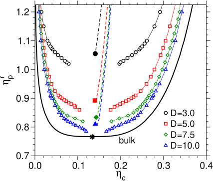
Figure 6: Coexistence curves of the AO model with $q=0.8$ in the bulk (full curve without data points, representing an extrapolation to the thermodynamic limit) and for thin films confined by symmetric walls, choosing Eq. (13) with $\varepsilon=0.5$ as a wall potential. Open circles denote data for $D=3$, $L=18$ (all lengths here are measured in units of the colloid diameter, $\sigma_{\rm c}=2R_{\rm c}$). Open squares denote data for $D=5$, $L=20$; open diamonds are for $D=7.5$, $L=30$ , and open triangles for $D=10$, $L=30$. The broken curves denote the corresponding coexistence diameters, $\eta_{\rm d}=(\eta^{\rm L}_{\rm c}+\eta^{\rm V}_{\rm c})/2$ and the full symbols denote estimates of the corresponding critical points for the various choices of $D$. From Vink et al. [62].

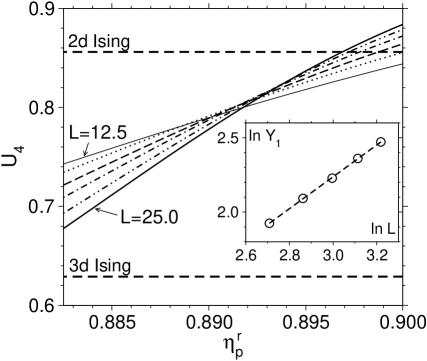
Figure 7: Moment ratio $U_{4}$ for a film of thickness $D=5$ plotted versus the polymer reservoir packing fraction $\eta^{\rm r}_{\rm p}$ and several choices of the lateral linear dimension, $L=12.5$, 15, 17.5, 20, 22.5, and 25. The intersection points allow to estimate the critical point as $\eta^{\rm r}_{\rm p,cr}=0.892\pm 0.002$. The inset shows a log-log plot of the slope $Y_{1}=dU_{4}/d\eta^{\rm r}_{\rm p}$ at $\eta^{\rm r}_{\rm p,cr}$ versus $L$, testing the prediction that $Y_{1}\propto L^{1/\nu}$. The straight line in the inset corresponds to an (effective) exponent $\nu_{\rm eff}=0.933$. The broken horizontal straight lines in the main part indicates the theoretical values for the universal value $U^{*}$ of $U_{4}$ at the intersection point, for both the $d=2$ and the $d=3$ Ising model, respectively. From Vink et al. [62].

These crossover phenomena make the analysis of the simulations somewhat more difficult. For any finite value of $L$ the “raw data” estimates for $\eta^{\rm V}_{\rm c}$, $\eta^{\rm L}_{\rm c}$ are qualitatively similar, irrespective of $D$ (Fig. 6). Again pronounced “finite size tails” occur for these estimates in the vicinity of $\eta^{\rm r}_{\rm p,cr}$, i.e., for any finite $L$ one finds that $\eta^{\rm V}_{\rm c}$ and $\eta^{\rm L}_{\rm c}$ as estimated from the peak positions of $P(\eta_{\rm c})$ fail to merge at $\eta^{\rm r}_{\rm p,cr}$, but rather continue further into the one-phase region, as in the bulk (Fig. 4). When one then plots $U_{4}$ vs. $\eta^{\rm r}_{\rm p}$ for different choices of $L$, searching for a universal intersection point, one rather finds that the intersection points are somewhat scattered over a region of values for $\eta^{\rm r}_{\rm p}$ (Fig. 7). In addition, this intersection does occur neither at the theoretical value for $U^{*}$ for the $d=2$ universality class nor at the $U^{*}$ for $d=3$, but rather somewhere in between. These findings are a consequence of the gradual crossover in critical behavior alluded to above. While for $D=3$ both $\nu$ and $U^{*}$ are rather close to the theoretical $d=2$ values, for $D=10$ both $\nu$ and $U^{*}$ are about half way between the $d=2$ and $d=3$ values. However, these numerical results do not have any fundamental significance; they only mean that the larger $D$ the closer $\eta^{\rm r}_{\rm p,cr}$ needs to be approached, to be in the region where ultimately $\xi\gg D$ and hence the correct asymptotic critical behavior (which is always two-dimensional, for any finite value of $D$) can be seen.

For the case $D=5$, $\varepsilon=0$ a very careful analysis has been performed [61], applying a novel variant of finite scaling which does not imply any bias on the type of critical exponents [117, 118, 119]. Fig. 8 shows that the resulting order parameter can be fitted over some range indeed by an effective exponent $\beta_{\rm eff}=0.17$, which is in between the $d=2$ and $d=3$ values (0.125 $<\beta_{\rm eff}<0.326)$, but a correct interpretation of this finding is that a log-log plot of the order parameter vs. $t$ exhibits a slight curvature, spread out over several decades. Only for $t\rightarrow 0$ can the $d=2$ value ($\beta=0.125)$ be expected to be seen; for larger $t$ the slope $\beta_{\rm eff}$ on the log-log plot increases systematically (but it does not reach the $d=3$ value, since for $t\geq 0.1$ noncritical saturation effects come into play).

While the critical behavior of thin films is controlled by the $d=2$ critical exponents, a different answer results when one considers the shift of the critical point relative to the bulk [33, 34]: this shift is controlled by three-dimensional exponents only, namely

$$\Delta\eta^{\rm r}_{\rm p,cr}(D) \equiv \eta^{\rm r}_{\rm p,cr}(D)-\eta^{\rm r}_{\rm p,cr}(\infty)$$ (15)

$$\propto D^{-1/\nu},\;D\to\infty$$

$$\Delta\mu^{\rm coex}_{cr}(D) \equiv \mu^{\rm coex}_{\rm cr}(D)-\mu^{\rm coex}_{\rm cr}(\infty)$$ (16)

$$\propto D^{(\Delta_{1}-\Delta)/\nu},\;D\to\infty.$$

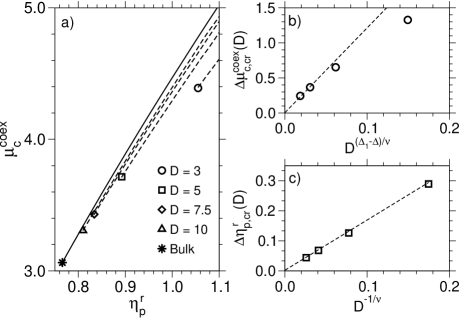
Figure 9: a) Coexistence curves of the AO model with $q=0.8$ in the grand-canonical representation where the chemical potential $\mu^{\rm coex}$ of the colloids at the coexistence curve is plotted vs. the polymer reservoir packing fraction $\eta^{\rm r}_{\rm p}$. The bulk result $(D=\infty)$ is shown as a full curve, while the broken curves show the coexistence curves for confined films for several thicknesses $D$, as indicated. The symbols mark the corresponding critical points. b) Shift of the critical coexistence colloid chemical potential plotted vs. $D^{(\Delta_{1}-\Delta)/\nu}$. Equation (16) implies a straight line, as indicated by the dashed curve. c) Shift of the critical polymer reservoir packing fraction, $\Delta\eta^{\rm r}_{\rm p,cr}(D)$, plotted vs. $D^{-1/\nu}$. The dashed lines indicate that Eq. (15) holds. From Vink et al. [62].

Here $\Delta\approx 1.56$ [97, 115, 116] is the so-called “gap exponent” which characterizes the bulk equation of state near criticality, and $\Delta_{1}\approx 0.47$ [120, 121, 122, 123] its surface analog. Figure 9 shows that the AO model is compatible with these predictions, even though only rather small film thicknesses were accessible to the simulation (the largest film thickness included in Fig. 9 is only for $D=10$ colloid diameters).

Note that for $\eta^{\rm r}_{\rm p}>\eta^{\rm r}_{\rm p,cr}$ the asymptotic behavior of the shift of the colloid chemical potential at phase coexistence is not given by Eq. (16), but by the simpler “Kelvin equation” [10, 35]

$$\Delta\mu^{\rm coex}(D) = \mu^{\rm coex}(D)-\mu^{\rm coex}(\infty)$$ (17)

$$\propto 1/D,\,D\rightarrow\infty,\,\eta^{\rm r}_{\rm p}>\eta^{\rm r}_{\rm p,cr}.$$

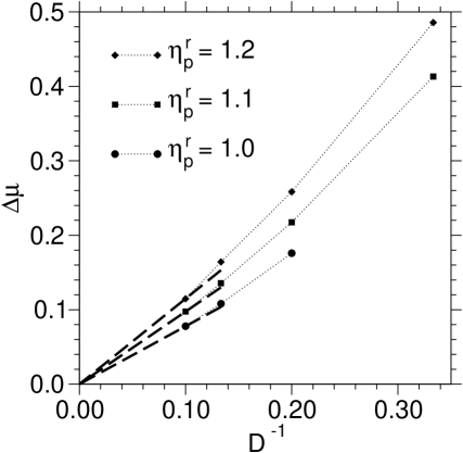
Figure 10: Test of the Kelvin equation. The chemical potential difference $\Delta\mu^{\rm coex}(D)$ {Eq. (17)} is plotted vs. $D^{-1}$ for three values of $\eta^{\rm r}_{\rm p}$, chosen well above the critical values $\eta^{\rm r}_{\rm p,cr}(D)$. Broken straight lines show that the data are compatible with the Kelvin equation. From Vink et al. [62].

Fig. 10 shows that the data of Vink et al. [62] are compatible with this equation as expected.

We emphasize that in mean field theory one could not discuss the crossover between two- and three-dimensional critical behavior, since $\beta_{\rm MF}=1$ irrespective of dimensionality [114], and also the mean-field predictions for the shift of the critical point [Eqs. (15), (16)] would be different from what was observed [62], since $1/\nu_{\rm MF}=2$ instead of $1/\nu\approx 1.59$, and ($\Delta^{\rm MF}_{1}-\Delta^{\rm MF})/\nu_{\rm MF}=-2$ instead of $(\Delta_{1}-\Delta)/\nu\approx-1.73$. However, mean-field theory does reproduce the Kelvin equation, Eq. (17), and in any case mean-field results for our confined films would be desirable. We note that some mean-field results as well as Monte Carlo results are available for $q=1$ [58, 59]; however, the accuracy of these Monte Carlo data was too limited to allow for a comprehensive test of theoretical predictions, as reviewed above, and hence these studies [58, 59] are not discussed further here.

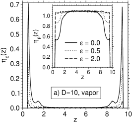
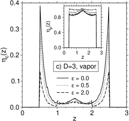
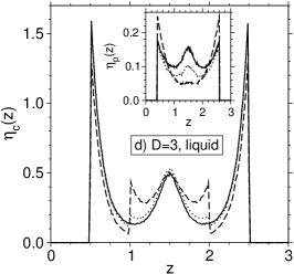
Figure 12: Colloid density profiles obtained in thin films at $\eta^{\rm r}_{\rm p}=1.1$, for two values of the film thickness $D$, and several values of the colloid-wall parameter $\varepsilon$ as indicated. Frames a) and b) show profiles obtained for $D=10$, on the vapor and liquid branch of the coexistence curve, respectively. Frames c) and d) show the corresponding profiles for thickness $D=3$. Note the jumps in the colloid density at $z=0.5,1.0,2.0,2.5$ caused through the jumps of the potential at $z=R_{\rm c}$ and $z=2R_{\rm c}$, respectively. The insets represent density profiles of the polymers. From Vink et al. [62].

We conclude this section by discussing the structure of the coexisting phases in the thin film in more detail. Already snapshot pictures [Fig. 11] show that in the $z$-direction the composition can be inhomogeneous. For $\varepsilon=0$ colloidal particles are enriched at the walls in the vapor-like phase, while for $\varepsilon=2$ polymers are enriched at the walls in the liquid-like phase. However, it would be wrong to consider these enrichment layers as wetting layers [24, 25, 26, 27]: wetting layers are macroscopically thick, and cannot occur in a thin film geometry [11]. One should also recall that wetting at the surface of a semi-infinite system occurs at bulk coexistence, while coexistence in the thin film deviates from bulk coexistence {cf. Eqs. (16), (17), and Figs. 9a, 10}. Fig. 12 shows density profiles across the thin film for several typical choices of parameters. One recognizes that the colloid density in the liquid -like phase near the walls shows a pronounced layering effect, while the polymer density in the vapor-like phase lacks a corresponding effect. This finding is expected, since layering is a consequence of the repulsive interactions among the particles. While for $D=10$ the films do reach homogeneous bulk-like states in their center, for $D=3$ and $D=5$ (not shown) the behavior stays inhomogeneous throughout the film.

4 Confinement by Asymmetric Walls: Evidence for an Interface Localization Transition

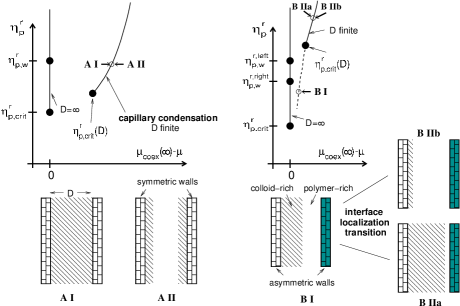
Figure 13: Schematic phase diagram of a colloid-polymer mixture confined between two parallel walls a distance $D$ apart, in the grand-canonical ensemble where the polymer reservoir packing fraction $\eta^{\rm r}_{\rm p}$ is used as ordinate and the difference between the chemical potential of the colloids at bulk phase coexistence $\mu_{\rm coex}(D=\infty)$ and the actual colloid chemical potential is used as abscissa. Thus, phase coexistence in the bulk occurs along a vertical straight line at $\mu_{\rm coex}(\infty)-\mu=0$. The left part shows the case of symmetric walls, the right part asymmetric walls. States AI and AII coexist along the capillary condensation transition line, states BIIa and BIIb coexist along the interface localization line, while state BI exists along the broken curve (which represents a line of rounded transitions). In the limit $D\rightarrow\infty$, which corresponds to an infinite system but bounded by walls both on the left and the right side, wetting transitions occur, that are rounded off for finite $D$. In the symmetric situation, the wetting transitions of both walls coincide at $\eta^{\rm r}_{\rm p,w}$, while in the asymmetric situation $\eta^{\rm r,right}_{\rm p,w}\neq\eta^{\rm r,left}_{\rm p,w}$. From De Virgiliis et al. [63].

By asymmetric walls one can realize a situation that one wall attracts predominantly colloids and the other wall attracts polymers. As discussed in the previous section, hard walls attract colloids via a depletion mechanism; but coating the wall by a polymer brush under semidilute conditions, one may cancel this depletion attraction partially or completely, and also reach a situation where polymers get attracted to the wall. This situation is qualitatively modelled by a step potential of height $\varepsilon$, acting on the colloids only {Eq. (13)}. An asymmetric situation occurs e.g. if the left wall is a hard wall but on the right wall the additional potential described by Eq. (13) acts, see Fig. (13). In drawing the schematic phase diagrams, we have assumed that for a semi-infinite system colloid-polymer mixtures exhibit complete wetting [11, 24, 25, 26, 27] over a wide range near the critical point, namely for $\eta^{\rm r}_{\rm p,cr}\leq\eta^{\rm r}_{\rm p}\leq\eta^{\rm r}_{\rm p,w}$, while for $\eta^{\rm r}_{\rm p}>\eta^{\rm r}_{\rm p,w}$ “incomplete wetting” (i.e., a nonzero contact angle of a droplet) would occur. This assumption is corroborated by density functional calculations [124] and Monte Carlo simulations [105, 125]. Since no “prewetting transition” [11, 24, 25, 26, 27] was found, the wetting transition presumably is of second order, and this was assumed drawing the phase diagrams of Fig. 13, since this greatly simplifies the theoretical analysis. For the case of symmetrical mixtures of long flexible macromolecules, the influence of prewetting phenomena on the phase diagram of thin confined films has been thoroughly investigated [11, 39, 65, 66, 67, 68, 69, 70, 71, 72], and it has been shown that typically a phase diagram with two critical points and a triple point can be expected.

For asymmetric walls an interface localization transition may occur, and this situation is explained qualitatively in the right part of Fig. 13. If the strength of the attraction of the colloids of the left wall is of the same order as the strength of the attraction of the polymers to the right wall, $\eta^{\rm r,right}_{\rm p,w}$ and $\eta^{\rm r,left}_{\rm p,w}$ will be rather close to each other and both exceed $\eta^{\rm r}_{\rm p,cr}$ distinctly. Then for $\eta^{\rm r}_{\rm p}>\eta^{\rm r}_{\rm p,cr}$ the left wall will always be coated with colloids, the right wall will always be coated with polymers. In other words, we expect an interface between the colloid-rich phase on the left and the polymer-rich phase on the right. When $\mu$ is small enough {i.e, $\mu_{\rm coex}(\infty)-\mu$ is large enough} most of the system is in the polymer-rich phase (shown schematically as BIIb in Fig. 13) but when $\mu$ increases a transition takes place to a state where most of the film is in the colloid-rich phase (state BIIa). For $\eta^{\rm r}_{\rm p}>\eta^{\rm r}_{\rm p,cr}(D)$ this transition is a sharp (first-order) phase transition, i.e. the interface jumps from a state localized at the left wall to a state localized at the right wall. For $\eta_{\rm p}^{\rm r}=\eta^{\rm r}_{\rm p,cr}(D)$ this transition is of first order, while for $\eta^{\rm r}_{\rm p}<\eta^{\rm r}_{\rm p,cr}(D)$ the transition is a smooth gradual transition (near the broken line in Fig. 13). Note, however, that this transition becomes sharper and sharper as $D$ increases, but a true phase transition appears only in a discontinuous manner in the limit $D\rightarrow\infty$ [11]: then the broken line in Fig. 13 coincides with the line $\mu=\mu_{\rm coex}(\infty)$ ending at $\eta^{\rm r}_{\rm p,cr}$ , and $\eta^{\rm r}_{\rm p,cr}(D)$ does not converge to $\eta^{\rm r}_{\rm p,cr}$ but rather we have $\eta^{\rm r}_{\rm p,cr}(D\rightarrow\infty)=\eta^{\rm r,left}_{\rm p,w}$ (for the situation drawn in Fig. 13).

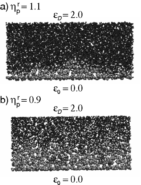
Figure 14: a) Snapshot picture of the polymer-rich phase, for $D=10$, $q=0.8$, $\eta^{\rm r}_{\rm p}=1.1$. The lower wall (at $z=0$) has a wall potential parameter energy $\varepsilon_{0}=0$ and hence attracts colloidal particles (shown in green), while the upper wall (at $z=D$) has a wall potential energy parameter $\varepsilon_{D}=2$, attracting polymers (shown in blue). b) Snapshot picture of the same system as in a), but for $\eta^{\rm r}_{\rm p}=0.9$ showing a state with a delocalized interface.

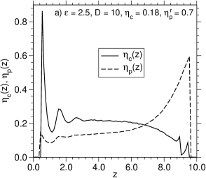
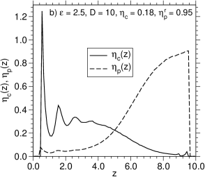
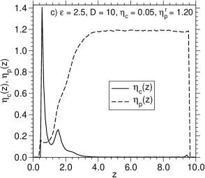
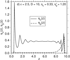
Figure 15: Colloid concentration profiles $\eta_{\rm c}(z)$ and polymer concentration profiles $\eta_{\rm p}(z)$ as a function of $z$ for a thin film with asymmetric walls (hard wall at $z=0$, while for the other wall at $z=D=10$ the potential $U_{\rm cw}(h)$ acts see Eq. (13), with $\varepsilon=2.5$). Profiles were obtained at $\eta_{\rm c}=0.18$, $\eta^{\rm r}_{\rm p}=0.70$ (a) , $\eta_{\rm c}=0.18$, $\eta^{\rm r}_{\rm p}=0.95$ (b), $\eta_{\rm c}=0.05$, $\eta^{\rm r}_{\rm p}=1.20$ (c), and $\eta_{\rm c}=0.33$, $\eta^{\rm r}_{\rm p}=1.20$ (d). For profiles (c) and (d), the choices $\eta_{\rm c}=0.05$, $0.33$ roughly correspond to the two branches of the coexistence curve, see Fig. 16. From De Virgiliis et al. [63].

For the states along the broken curve in Fig. 13 the system is essentially inhomogeneous, there exists a thick domain of colloid-rich phase in the left part of the film, and a thick domain of polymer-rich phase in the right part, separated by a “delocalized” interface in the center of the film [11, 36, 37, 38, 39]. Snapshot pictures of the system indeed readily confirm such a scenario (Fig. 14), as well as the density profiles across the thin film (Fig. 15). Fig. 15a shows the profile for $\eta^{\rm r}_{\rm p}=0.7<\eta^{\rm r}_{\rm p,cr}$, i.e. a state in the one phase region of the bulk. One recognizes that the colloid concentration is enhanced near the hard wall, as expected from the depletion attraction. Near the other wall at $z=D=10$, the colloid concentration is somewhat depressed, but the polymer concentration is clearly enhanced. But in the center of the thin film both profiles are roughly constant, as expected for bulk-like behavior. In fact, for large $D$ we expect that the surface enhancement (or reduction, respectively) decays with $z$ according to an exponential relation, $\exp(-h/\xi)$, where $h$ is the distance from the closest wall and $\xi$ the bulk correlation length [120]. Figure 15b shows the profiles at $\eta^{\rm r}_{\rm p}=0.95$, which exceeds the bulk critical value $\eta^{\rm r}_{\rm p,cr}$, but still is smaller than the critical value $\eta^{\rm r}_{\rm p,cr}(D)$ of the confined system. Now, the profiles are very different from those of Fig. 15a: phase separation in a colloid-rich and a polymer-rich phase has occurred, with the interface position (estimated from the inflection point of the polymer volume fraction profile $\eta_{\rm p}(z)$, for instance) being located in the center of the film. This situation corresponds to the snapshot in Fig. 14b. The interfacial profile resembles that of an interface between bulk coexisting phases, broadened by capillary waves [68, 83]. Finally, the cases $\eta^{\rm r}_{\rm p}=1.2$ (Fig. 15c,d) refer to the two-phase region of the film. The interface either is located near the hard wall, corresponding to the polymer-rich phase of the film (Fig. 15c: this case corresponds to the snapshot shown in Fig. 14a), or near the wall that attracts the polymers (Fig. 15d). Note that along the transition line drawn schematically in Fig. 13 (right part), there occurs lateral phase separation between the states corresponding to these two types of profiles, Fig. 15c and Fig. 15d, which hence can coexist with each other in a thin film (and then are separated by an interface running from the right wall towards the left wall).

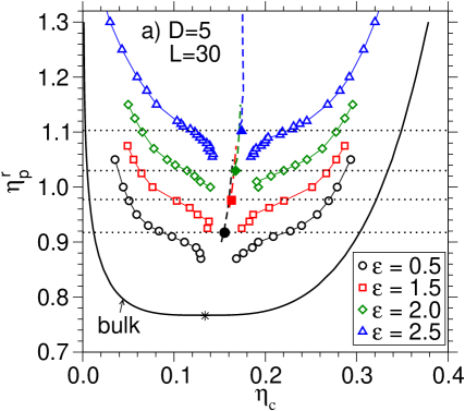
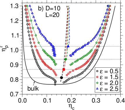
Figure 16: Coexistence curves for $D=5$, $L=30$ (a) and $D=10$, $L=20$ (b), using four values of $\varepsilon$, as indicated. Also the bulk coexistence curve is shown (full curves). Full symbols mark critical points, the broken lines ending at these critical points are the coexistence diameters. The dotted horizontal straight lines mark the values of $\eta^{\rm r}_{\rm p,cr}(D)$. From De Virgiliis et al. [63].

Figure 16 shows the corresponding phase diagrams for two film thicknesses, $D=5$ and $D=10$, varying the strength $\varepsilon$ of the potential [Eq. (13)] at the right wall. One sees that with increasing $\varepsilon$ the critical points and the whole coexistence curves are shifted upwards, to rather large values of $\eta^{\rm r}_{\rm p}$. This shift is consistent with the qualitative phase diagram of Fig. 13 (right part). Of course, one must again recall that in Fig. 16 we show “raw Monte Carlo data” for one choice of $L$ only, and hence pronounced finite size tails near $\eta^{\rm r}_{\rm p,cr}(D)$ are apparent, as discussed for the case of capillary condensation already (Fig. 6). The critical points were again estimated from the cumulant intersection method. Although strong corrections to scaling are present, the conclusion can be drawn [63] that the critical behavior of the interface localization belongs to the $d=2$ Ising universality class, as expected [36, 37, 38].

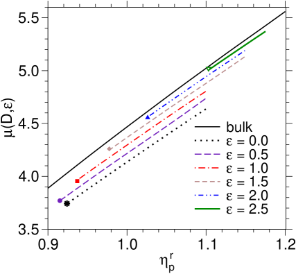
Figure 17: Phase diagram of a thin film of colloid-polymer mixtures with asymmetric walls in the grand-canonical ensemble, choosing $q=0.8$, $D=5$, with $\eta^{\rm r}_{\rm p}$ as abscissa and $\mu$ as ordinate. Curves show the coexistence potential $\mu_{\rm coex}(D,\varepsilon)$ of the colloids. Full curve denotes the result for the bulk (note that the bulk critical point, $\eta^{\rm r}_{\rm p,cr}=0.766$ is off the scale of this figure). Full symbols mark the critical points of the films. From De Virgiliis et al. [63]

Figure 17 shows the phase diagram for $D=5$ and various choices of $\varepsilon$ in the grand-canonical representation (this is the counterpart of Fig. 9a for capillary condensation, where $D$ was varied for $\varepsilon=0$, while here we study the variation with $\varepsilon$ at fixed $D$). One can see that by increasing $\varepsilon$ the coexistence curves of the thin film move closer towards the bulk coexistence curves, and for $\varepsilon=2.5$ the deviation from the bulk indeed is very small, but the critical point is strongly shifted (from $\eta^{\rm r}_{\rm p,cr}=0.766$ in the bulk to $\eta^{\rm r}_{\rm p,cr}=1.106$ in the thin film).

This behavior is qualitatively similar to what has been found for the Ising ferromagnet with competing surface magnetic fields [11, 38], the generic model for which the interface localization transition was studied for the first time.

Note that the curve for $\varepsilon=0$ in Fig. 17 represents capillary condensation (and a similar conclusion applies to the case $\varepsilon=0.5$ as well). Figure 17 implies that varying $\varepsilon$ one can completely smoothly cross over from capillary condensation-like behavior to interface localization-like behavior, when $\varepsilon$ is increased. In view of the qualitative description of Fig. 13 this is somewhat surprising: in the capillary condensation transition, the two liquid-vapor interfaces bound to the walls annihilate each other, the slit pore gets almost uniformly filled with liquid. In the interface localization transition, one has an interface on both sides of the transition, it just has jumped at the transition from one wall to the other.

How can one then reconcile Figs. 13 and 17 with each other? The clue to the problem is, of course, that the picture of the states in Fig. 13 is far too simplified, it ignores the variations of the densities close to the wall. Therefore the states with “interfaces bound to walls” are a simplification, which lose its meaning when the “phase” in between the interface and the wall can no longer be clearly identified with bulk-like properties (as is actually the case, see Fig. 15). While one can clearly imagine to transform the left phase diagram of Fig. 13 into the right one by smooth changes, one should not take the sketches that illustrate the character of the phases too literally. The failure of these sketches, however, also means that one must be careful with all approaches where wetting phenomena and interface localization transitions [24, 25, 26, 27, 36, 37, 38] are simply described in terms of the “interface hamiltonian” picture, since according to this description the distance $\ell$ of the interface from the wall is the single degree of freedom (on a mean-field level) left to analyze the problem.

5 Summary and Outlook

In this brief review we have emphasized that confinement has very interesting effects on soft matter systems, both with respect to the structure and the phase behavior of these systems. Of course, confinement also has very interesting consequences on the dynamics of soft matter systems (see e.g. [13, 14, 15, 16, 17, 18, 19] for recent discussions), but this aspect has been completely outside of the focus of our review.

We also have focused on the case which we consider to be the simplest case, confinement between two flat and ideally parallel walls a finite distance $D$ apart. Practically more important, of course, is the confinement in random porous media [10, 12, 20, 21, 22, 23]. However, in this case the random irregularity of the confining geometry is a serious obstacle for a detailed understanding. There is ample evidence (both from experiment [126, 127] and simulations [128, 129, 130]) that the liquid-vapor type phase separation or demixing of binary fluid mixtures under such confinement is seriously modified, but the character of this modification has been under discussion since a long time [126, 127, 128, 129, 130, 131, 132]. De Gennes [131] argued that due to the random arrangement of the pore walls (which prefer one of the coexisting phases over the other) the problem can be mapped to the random field Ising model [133, 134]. While for a long time the existing evidence [126, 127, 128, 129, 130] was inconsistent with this suggestion, in recent work on colloid-polymer mixtures confined by a fraction of colloids that are frozen in their positions and do not take part in the phase separation, evidence for the random field Ising behavior was obtained [132]. Note that then it is necessary to reach a regime where the correlation length has grown to a large enough distance, much larger than the characteristic linear dimension of the confining particles.

Another case, that has received ample consideration in the literature (see [12] for further references) but was disregarded here, is the confinement in a quasi-one-dimensional cylindrical geometry. In this case again the structure is typically inhomogeneous in the radial direction perpendicular to the walls of the cylinder. The correlation length can grow indefinitely only in one direction, along the cylinder axis, however. Therefore the phase transition to this laterally segregated state is a gradual (rounded) transition only, and even for conditions where in the bulk the system is strongly segregated (with an interfacial tension $\gamma$ between the coexisting phases which is not small in comparison with $k_{B}T$), there is no macroscopic phase separation possible: rather one predicts that only phase separation into domains of finite size can occur (cross sectional area $A$ of the cylinder and length $\ell_{\rm d}$ of the domains), where [135, 136] $\ln\ell_{d}\propto A\gamma/k_{B}T$. This happens because thermal fluctuations prevent the establishment of true long range order by the spontaneous generation of transverse interfaces (across the cylinder). This has the consequence that also, in principle, the capillary condensation or evaporation transitions in cylindrical geometry are, in full thermal equilibrium, not perfectly sharp but rounded. In practice, this effect often is masked by nonequilibrium phenomena (pronounced hysteresis occurs!) and hence we are not aware of careful studies where this rounding has been demonstrated. Note that mean-field treatments [12] miss such fluctuations effects, of course. Also, when one considers cylindrical geometries with “‘competing walls” (e.g. a cylinder with a square cross section, where the upper walls prefer one phase and the lower walls prefer the other phase [137, 138]) the interface localization transition in such a “double wedge”-geometry is rounded and not sharp, as simulations show where one considers the limit that the length of the cylinder gets macroscopic while its cross section stays finite [138]. Since recently it has become possible to create artificial cylindrical nanochannels with diameters between 35 and 150 nm [139], it would be interesting to study phase separation in such nanochannels experimentally as well.

Using the AO model of colloid-polymer mixtures as an example that is well suited for simulation studies [61, 62, 63], we have discussed simulation evidence for the theoretical concepts on capillary condensation and interface localization transitions [11, 33, 34, 35, 36, 37, 38]. In particular, the predictions for the shift of the critical point have been found to be compatible with the simulation results, and it was also argued that the critical behavior of the lateral phase separation in the thin film has the character of the two-dimensional Ising model (although in practice one is mostly in a crossover region where “effective exponents” in between the $d=2$ and $d=3$ limits apply, which do not have a deep theoretical significance). Clearly, it would be nice to have also experiments that confirm the findings of theory and simulation on the phase behavior of confined fluid mixtures.

One crucial assumption of the work reviewed here was that the wetting transitions (that occur in the limit when the film thickness $D$ diverges to infinity) are of second order [11]. If first-order wetting occurs, much more complicated phase diagrams under confinement result [11]. To some extent, this problem has been worked out for symmetrical polymer blends under confinement [65, 66, 67, 68, 69, 70, 71, 72], and we refer the reader to these papers for details. In particular, it also should be possible to realize situations in between capillary condensation and interface localization transitions [67].

Finally, we draw attention to more complicated ordering phenomena under confinement. A problem that has found a lot of attention is the effect of confinement in thin films on the blockcopolymer mesophase ordering [140, 141, 142, 143]. For more or less symmetric composition of a diblock copolymer, the mesophase observed in the bulk is a lamellar ordering [57]. The question that is then discussed in the literature (both experimentally and theoretically, see [140, 141, 142] for further references), is whether the lamellae are oriented parallel or perpendicular to the confining walls, and transitions in the number of lamellae that fit into the thin film, etc. (remember that the lamella thickness depends on temperature, chain length of the polymers, and other control parameters [57]). For asymmetric compositions $A_{f}B_{1-f}$ of a diblock copolymer, however, already in the bulk melts other mesophases appear, such as hexagonal patterns of A-rich cylinders in B-rich background, or cubic structures, where A-rich cores of micelles form a periodic lattice in the B-rich background, or vice versa [57]. For triblock copolymers, many much more complex mesophases occur, and the question how all this self-assembly of block copolymers is affected by confinement due to walls is still under both theoretical and experimental investigation (see e.g. [143]).

Other very interesting confinement effects in soft matter occur when orientational order is involved, e.g. when a colloidal dispersion undergoing a transition from isotropic to nematic phases is confined by walls (see e.g. [144, 145, 146, 147]). Confinement may enhance the nematic ordering tendency (“capillary nematization” [144] is the analog phenomenon of capillary condensation), but one needs also to take into account the tensor character of the order parameter of liquid crystals. Thus near a wall a biaxial character of the ordering occurs even when in the bulk the ordering is uniaxial. Also the boundary conditions at the walls can be envisaged such that one wall prefers parallel and the other wall perpendicular alignment, leading to a tilted structure of the ordering across the film [145]. These remarks are by no means intended as an exhaustive discussion, but just want to draw the attention of the reader to this wealth of interesting problems.

Acknowledgments: Support from the Deutsche Forschungsgemeinschaft (DFG) via SFB TR6/A5 is gratefully acknowledged. We are indebted to S. Dietrich, R. Evans, H. Lekkerkerker, H. Löwen, M. Müller, M. Schmidt and P. Virnau for many stimulating discussions.

Figure 1: Phase diagram of the AO model with a size ratio $q=R_{\rm p}/R_{\rm c}=0.8$ plotted in the $(\eta_{\rm p},\eta_{\rm c})$ plane, showing the coexistence curve for phase separation into a polymer-rich phase (left) and a colloid-rich phase (right), according to Monte Carlo (circles) and the free volume mean-field theory of Lekkerkerker et al. (full line) [75]. The Monte Carlo data were obtained using a simulation box with linear dimensions $L_{x}=L_{y}=16.7$, $L_{z}=33.4$ (some data for a smaller box with $L_{x}=L_{y}=13.3$, $L_{z}=26.5$ are also included as crosses). The solid square shows the estimate for the critical point as obtained from a finite size scaling analysis of the Monte Carlo data, cf. text. The insert shows the same data, in the so-called “reservoir representation” where $\eta^{\rm r}_{\rm p}$ rather than $\eta_{\rm p}$ is used as a variable. The one-phase region where colloids and polymers are fully miscible is always shown in the lower parts of these diagrams, below the coexistence curves. From Vink and Horbach [81].

Figure 2: Logarithm of the probability $P(\eta_{\rm c})$ of observing a colloid packing fraction $\eta_{\rm c}$ for an AO mixture with $q=0.8$ at coexistence for several values of $\eta^{\rm r}_{\rm p}$ as indicated. The simulations were performed in a box with linear dimensions $L_{x}=L_{y}=16.7$ and $L_{z}=33.4$ using periodic boundary conditions. Note that the distributions are not normalized, and that for $\eta$ near $\eta_{\rm d}=(\eta^{\rm V}_{\rm c}+\eta^{\rm L}_{\rm c})/2$ the distribution is essentially flat, almost independent from $\eta_{\rm c}$, so that a free energy barrier $\Delta F$ is well-defined. From Vink and Horbach [81].

Figure 3: Reduced interfacial tension $\gamma^{*}=4R^{2}_{\rm c}\gamma_{\rm LV}/k_{B}T$ for an AO mixture with $q=0.8$ as a function of the difference in packing fraction between the coexisting phase, $\eta^{\rm L}_{\rm c}-\eta^{\rm V}_{\rm c}$. The inset shows $\gamma^{*}$ vs. $\eta^{\rm r}_{\rm p}$. Open circles are the simulation results, while the full curves are density functional theory predictions. From Vink and Horbach [81]

Figure 4: Close-up of the phase diagram of the AO model for $q=0.8$ in the critical region, showing only the range $0.75\leq\eta^{\rm r}_{\rm p}\leq=0.80$ for the polymer reservoir packing fraction. Results for four different choices of the linear dimension $L$ of $L\times L\times L$ simulation boxes are shown as broken and dotted lines. The extrapolation towards the thermodynamic limit, $L=\infty$, also is included, and the estimate for the critical point $\eta^{\rm r}_{\rm p,cr}=0.766\pm 0.002$ is shown by the error bar. From Vink et al. [82]

Figure 5: Scaling plot for the order parameter $M_{\rm c}=\langle|m|\rangle$ of the colloid-polymer mixture in the bulk, for the AO model with $q=0.8$, using only data for $t>0$. The quantity $L^{\beta/\nu}M_{\rm c}$ is plotted vs. $tL^{1/\nu}$, choosing logarithmic scales. The straight line is a power law $y=0.27x^{\beta}$, with $\beta=0.326$. From Vink et al. [83].

Figure 8: Order parameter $\Delta(=M_{\rm c})$ of the confined AO model with $q=0.8$ plotted vs. $\eta^{\rm r}_{\rm p}$, choosing $D=5$ and $\varepsilon=0$. The curve through the simulation data in the main frame is a fit to $\Delta=B_{\rm eff}t^{\beta_{\rm eff}}$, choosing $\eta^{\rm r}_{\rm p,cr}=0.9223$. The inset shows the same data as a function of the relative distance from the critical point, $t=\eta^{\rm r}_{\rm p}/\eta^{\rm r}_{\rm p,cr}-1$, on double logarithmic scales; broken straight lines illustrate the two-dimensional and three dimensional Ising exponents. From Vink et al. [61].

Figure 11: Snapshot pictures of coexisting phases for the colloid-polymer mixture with $q=0.8$, $D=10$, $\eta^{\rm r}_{\rm p}=1.1$, for $\varepsilon=0$ (a) and $\varepsilon=2.0$ (b) Colloidal particles are in green, polymers in blue (the size of the polymers is rescaled to allow a clearer view).

References

- [1] G. Decker and J.B. Schlenoff (eds.) Multilayer Thin Films: Sequential Assembly of Nanocomposite Materials, 2002, Wiley-VCH, Weinheim.
- [2] E.L. Wolf Nanophysics and Nanotechnology, 2004, Wiley-VCH, Weinheim.
- [3] Y. Champion and H.J. Fecht (eds.) Nano-Architectured and Nano-Structured Materials, 2004, Wiley-VCH, Weinheim.
- [4] C.N.R. Rao, A. Müller, and A.K. Cheetham (eds.) The Chemistry of Nanomaterials, 2004, Wiley-VCH, Weinheim.
- [5] R. Kelsall, I.W. Hamley and M. Geohegan (eds.) Nanoscale Science and Technology, 2005, Wiley-VCH, Weinheim.
- [6] J.S. Rowlinson and B. Widom, Molecular Theory of Capillarity, 1982, Oxford University Press, Oxford.
- [7] C.A. Croxton (ed.) Fluid Interfacial Phenomena, 1985, Wiley, New York.
- [8] I. Charvolin, J.-F. Joanny, and J. Zinn-Justin (eds.) Liquids at Interfaces, 1990, North Holland, Amsterdam.
- [9] D. Henderson (ed.) Fundamentals of Inhomogeneous Fluids, 1992, M. Dekker, New York.
- [10] L.D. Gelb, K.E. Gubbins, R. Radhakrishnan, and M. Sliwinska-Bartkowiak. Rep. Prog. Phys., 1999, 62, 1573-1659.
- [11] K. Binder, D.P. Landau, and M. Müller, J. Stat. Phys., 2003, 110, 1411-1514.
- [12] M. Schön and S. Klapp, Rev. Comp. Chem., Vol. 24, 2007, Wiley-VCH, Hoboken.
- [13] B. Frick, R. Zorn, and H. Büttner (eds.) International Workshop on Dynamics in Confinement. J. Phys. IV, 2000, 10.
- [14] B. Frick, M. Koza, and R. Zorn (eds.) 2nd International Workshop on Dynamics in Confinement, 2003, Eur. Phys. J. E 12, Nr. 1.
- [15] M. Koza, B. Frick, and R. Zorn (eds.) 3rd International Workshop on Dynamics in Confinement, 2007, Eur. Phys. J. ST, 141.
- [16] A. Meller, J. Phys.: Condens. Matter, 2003, 15, R581.
- [17] T.M. Squires and S.R. Quake, Rev. Mod. Phys., 2005, 77, 977.
- [18] D.I. Dimitrov, A. Milchev, and K. Binder, Phys. Rev. Lett., 2007, 99, 054501, 1-4.
- [19] D.I. Dimitrov, A. Milchev, and K. Binder, Langmuir, 2008.
- [20] S.J. Gregg and K.S.W. Sing, Adsorption, Surface Area, and Porosity, 2nd, ed. 1982, Academic Press, New York.
- [21] A.J. Liapis (ed.) Fundamentals of Adsorption, Engineering Foundation. 1987, New York.
- [22] J. Fraissard (ed.) Physical Adsorption: Experiment, Theory and Applications, 1997, Kluwer Acad. Publ., Dordrecht.
- [23] F. Rouquerol, J. Rouquerol, and K.S.W. Sing, Adsorption by Powders and Porous Solids: Principles, Methodology and Applications, 1999, Academic Press, San Diego.
- [24] P.G. de Gennes, Rev. Mod. Phys., 1985, 57, 825.
- [25] D.E. Sullivan and M.M. Telo da Gama, in Ref. [7], 45.
- [26] S. Dietrich, in Phase Transitions and Critical Phenomena, Vol 12, ed. by C. Domb and J.L. Lebowitz. 1988, New York, Academic, 1-218.
- [27] M. Schick, in Ref. [8], 415.
- [28] V.P. Privman (ed.) Finite Size Scaling and the Numerical Simulation of Statistical Systems, 1990, World Scientific, Singapore.
- [29] K. Binder, Ann. Rev. Phys. Chem., 1992, 42, 33-59.
- [30] K. Binder, in Computational Methods in Field Theory, ed. by C.B. Lang and H. Gausterer. 1992, Springer, Berlin, 59-125.
- [31] A. Patrykiejew, S. Sokolowski, and K. Binder, Surf. Sci. Rep., 2000, 37, 207-344.
- [32] J.L. Salamacha, A. Patrykiejew, S. Sokolowski, and K. Binder, J. Chem. Phys., 2005, 122, 074703.
- [33] M.E. Fisher and H. Nakanishi, J. Chem. Phys., 1981, 75, 5857-5863.
- [34] H. Nakanishi and M.E. Fisher, J. Chem. Phys., 1983, 78, 3279.
- [35] R. Evans, J. Phys.: Condens. Matter, 1990, 2, 8989.
- [36] A.O. Parry and R. Evans, Phys. Rev. Lett., 1990, 64, 439-442.
- [37] A.O. Parry and R. Evans, Physica A, 1992, 181, 250-296.
- [38] K. Binder, R. Evans, D.P. Landau, and A.M. Ferrenberg, Phys. Rev. E, 1996, 53, 5023-5034.
- [39] M. Müller, K. Binder, and E.V. Albano, Physica A, 2000, 279, 188-194.
- [40] W. Poon, J. Phys.: Condens. Matter, 2002, 14, R859-R880.
- [41] T. Kerle, J. Klein, and K. Binder, Phys. Rev. Lett., 1996, 77, 1318-1321.
- [42] T. Kerle, J. Klein, and K. Binder, Eur. Phys. J. B, 1999, 7, 401-410.
- [43] A.v. Blaaderen, Prog. Colloid Polymer Sci., 1997, 104, 59.
- [44] D.G.A.L. Aarts, J.H. van der Wiel, and H.N.W. Lekkerkerker, J. Phys.: Condens. Matter, 2003, 15, S245.
- [45] D.G.A.L. Aarts, M. Schmidt, and H.N.W. Lekkerkerker, Science, 2004, 847.
- [46] W.C. Poon and P.N. Pusey, in Observation, Prediction and Simulation of Phase Transitions in Complex Fluids, edited by M. Baus, L.F. Rull, and J.P. Ryckaert, Kluwer Acad. Publ., 1995, Dordrecht.
- [47] A.K. Arora and B.V.R. Tata Adv. Colloid Int. Sc., 1998, 78, 49.
- [48] H. Löwen, J. Phys.: Condens. Matter, 2001, 13, R415.
- [49] A. Halperin, M. Tirrell, and T.P. Lodge, Adv. Polym. Sci., 1991, 100, 31.
- [50] G.S. Grest and M. Murat, in Monte Carlo and Molecular Dynamics Simulations in Polymer Science, ed. by K. Binder., 1995, Oxford Univ. Press, 476.
- [51] S. Granick (Eds.) Polymers in Confined Geometries. Adv. Polym. Sci., 1999, 138.
- [52] R.C. Advincula, W.J. Brittain, R.C. Caster and J. Rühe (eds.) Polymer Brushes, 2004, Wiley-VCH, Weinheim.
- [53] D.H. Napper, Polymeric Stabilization of Colloidal Dispersions, 1983, Academic Press, London.
- [54] A. Budkowski, Adv. Polymer Sc., 1999, 148, 1-112.
- [55] P.J. Flory, Principles of Polymer Chemistry, 1993, Cornell Univ. Press, Ithaca, N.Y.
- [56] P.G. de Gennes, Scaling Concepts in Polymer Physics, 1979, Cornell Univ. Press, Ithaca.
- [57] K. Binder, Adv. Polym. Sc., 1994, 112, 181-299.
- [58] M. Schmidt, A. Fortini, and M. Dijkstra, J. Phys.: Condens. Matter, 2003, 15, S3411-S3420.
- [59] M. Schmidt, A. Fortini, and M. Dijkstra, J. Phys.: Condens. Matter, 2004, S4159-S4168.
- [60] A. Fortini, M. Schmidt, and M. Dijkstra, Phys. Rev. E, 2006, 73,051502, 1.
- [61] R.L.C. Vink, K. Binder, and J. Horbach, Phys. Rev. E, 2006, 73, 056118, 1-11.
- [62] R.L.C. Vink, A. De Virgiliis, J. Horbach, and K. Binder, Phys. Rev. E, 2006, 74, 031601, 1-72, Erratum, ibid.
- [63] A. De Virgiliis, R.L.C. Vink, J. Horbach, and K. Binder, Europhys. Lett., 2007, 77, 60002, 1-6.
- [64] S. Jungblut, T. Tuinier, K. Binder, and T. Schillng, J. Chem. Phys., 2007, 127, 24909, 1-9.
- [65] M. Müller and K. Binder, Macromolecules, 1998, 31, 8326-8346.
- [66] M. Müller, E.V. Albano, and K. Binder, Phys. Rev. E, 2000, 62, 5218-5296.
- [67] M. Müller, K. Binder, and E.V. Albano, Europhys. Lett., 2000, 50, 724-730.
- [68] A. Werner, F. Schmid, M. Müller, and K. Binder, J. Chem. Phys., 1997, 107, 8175-8188.
- [69] A. Werner, M. Müller, F. Schmid, and K. Binder, J. Chem. Phys., 1999, 110, 1221-1229.
- [70] M. Müller and K. Binder, Phys. Rev. E, 2001, 63, 021602, 1-16.
- [71] M. Müller and K. Binder, J. Phys.: Condens. Matter, 2005, 17, S333-S361.
- [72] M. Müller and K. Binder, Int. J. Thermophys., 2006, 27, 448-466.
- [73] S. Asakura and F. Oosawa, J. Chem. Phys., 1954, 22, 1255-1256.
- [74] A. Vrij, Pure App. Chem., 1976, 48, 471.
- [75] H.N.W. Lekkerkerker, W. Poon, P. Pusey, A. Stroobants, and P. Warren, Europhys. Lett., 1992, 20, 559.
- [76] A.A. Louis, R. Finken, and J.-P. Hansen, Europhys. Lett., 1999, 46, 741.
- [77] M. Dijkstra, J.M. Brader, and R. Evans, J. Phys.: Condens. Matter, 1999, 11, 10079.
- [78] M. Schmidt, H. Löwen, J. Brader, and R. Evans, Phys. Rev. Lett., 2000, 85, 1934-1937.
- [79] R.G. Bolhuis, A.A. Louis, and J.-P. Hansen, Phys. Rev. Lett., 2002, 89, 128302, 1-4.
- [80] R.L.C. Vink and J. Horbach, J. Chem. Phys., 2004, 121, 3253-3258; see also http://xxx.lanl.gov/abs/cond-mat/0402585.
- [81] R.L.C. Vink and J. Horbach, J. Phys.: Condens. Matter, 2004, 16, S3807-S3820.
- [82] R.L.C. Vink, J. Horbach, and K. Binder, Phys. Rev. E, 2005, 71, 011401, 1-10.
- [83] R.L.C. Vink, J. Horbach, and K. Binder, J. Chem. Phys., 2005, 122, 134905, 1-11.
- [84] P.G. Bolhuis and A.A. Louis, Macromolecules, 2002, 35, 1860.
- [85] E.J. Meijer and D. Frenkel, J. Chem. Phys., 1994, 100, 6873.
- [86] M. Fuchs and K.S. Schweizer, J. Phys.: Condens. Matter, 2002, 14, R239.
- [87] S. Ramakrishnan, M. Fuchs, K.S. Schweizer, and C.F. Zukoski, J. Chem. Phys., 2002, 116, 2201.
- [88] M. Schmidt, A.R. Denton, and J.M. Brader, J. Chem. Phys., 2003, 118, 1541.
- [89] R.L.C. Vink and M. Schmidt, Phys. Rev. E, 2005, 71, 051406, 1.
- [90] A. Jusufi, J. Dzubiella, C.N. Likos, C. von Ferber, and H. Löwen, J. Phys.: Condens. Matter, 2001, 13, 6177.
- [91] J. Dzubiella, C.N. Likos, and H. Löwen, J. Chem. Phys., 2002, 116, 9518.
- [92] R. Rotenberg, J. Dzubiella,, A.A. Louis, and J.-P. Hansen, Mol. Phys., 2004, 102, 1.
- [93] E.H.A. de Hoog and H.N.W. Lekkerkerker, J. Phys. Chem. B, 1999, 103, 5274.
- [94] A.R. Denton and M. Schmidt, J. Chem. Phys., 2005, 122, 244911, 1.
- [95] A. Fortini, M. Dijkstra, and R. Tuinier, J. Phys.: Condens. Matter, 2005, 17, 7783.
- [96] W.K. Wijting, W. Knoben, N.A.M. Besseling, F.A.M. Leermakers, and M.A.C. Stuart, Phys. Chem. Chem. Phys., 2004, 6, 4432.
- [97] K. Binder and E. Luijten, Phys. Rep., 2001, 344, 179-253.
- [98] N.B. Wilding, in Ann. Rev. Comp. Phys., Vol IV, edited by D. Stauffer. 1996, World Scientific, Singapore, 37.
- [99] K. Binder, Rep. Prog. Phys., 1997, 60, 487-559.
- [100] D.P. Landau and K. Binder, A Guide to Monte Carlo Simulations in Statistical Physics, 2000, Cambridge Univ. Press, Cambridge.
- [101] P.C. Hohenberg and B.I. Halperin, Rev. Mod. Phys., 1977, 49, 435.
- [102] M.E. Fisher, in Critical Phenomena, edited by M.S. Green, 1971, New York, 1.
- [103] K. Binder, Z. Phys. B: Condens. Matter, 1981, 43, 119-140.
- [104] A.Z. Panagiotopoulos, Mol. Phys., 1987, 61, 813.
- [105] M. Dijkstra and R. van Roi, Phys. Rev. Lett., 2002, 89, 208303, 1-4.
- [106] K. Binder and D. P. Landau, Phys. Rev. B, 1984, 30, 1477-1485.
- [107] C. Borgs and R. Kotecky, J. Stat. Phys., 1990, 61, 79.
- [108] P. Virnau and M. Müller, J. Chem. Phys., 2004, 120, 10925.
- [109] K. Binder, Phys. Rev. A, 1982, 25, 1699-1709.
- [110] M. Schmidt, private communication.
- [111] G. Kamieniarz and H.W.J. Blöte, J. Phys. A, 1993, 26, 201.
- [112] H.-P. Deutsch, J. Stat. Phys., 1992, 67, 1039.
- [113] E. Luijten, M.E. Fisher, and A.Z. Panagiotopoulos, Phys. Rev. Lett., 2002, 88, 185701, 1-4.
- [114] M.E. Fisher, Rev. Mod. Phys., 1974, 46, 587.
- [115] M.E. Fisher and S.-Y. Zinn, J. Phys. A, 1998, 26, 201.
- [116] J. Zinn-Justin, Phys. Rep. 2001, 344, 159-178.
- [117] Y.C. Kim, M.E. Fisher, and E. Luijten, Phys. Rev. Lett., 2001, 91, 065701, 1-4.
- [118] Y.C. Kim and M.E. Fisher, Comp. Phys. Comm., 2005, 169, 295.
- [119] Y.C. Kim, Phys. Rev. E, 2005, 71, 051501, 1.
- [120] K. Binder, in Phase Transition and Critical Phenomena Vol 8, edited by C. Domb and J.L. Lebowitz, 1983, Academic Press, London, 1-144.
- [121] K. Binder and D.P. Landau, Phys. Rev. Lett., 1984, 52, 318-321.
- [122] C. Ruge and F. Wagner, Phys. Rev. B, 1995, 52, 4209.
- [123] H.W. Diehl and M. Shpot, Nucl. Phys. B, 1998, 528, 595.
- [124] J. Brader, R. Evans, M. Schmidt, and H. Löwen, J. Phys.: Condens. Matter, 2003, 14, L1.
- [125] M. Dijkstra, R. van Roij, R. Roth and A. Fortini, Phys. Rev. E, 2006, 73, 041404.
- [126] A.P.Y. Wong and M.H.W. Chan, Phys. Rev. Lett., 1990, 65, 2567-2570.
- [127] A.P.Y. Wong, S.B. Kim, W.I. Goldburg, and M.H.W. Chan, Phys. Rev. Lett., 1993, 70, 954-957.
- [128] M. Álvarez, D. Levesque, and J.J. Weis, Phys. Rev. E, 1999, 60, 5495.
- [129] L. Sarkisov and P.A. Monson, Phys. Rev. E, 2000, 61, 7231.
- [130] V. De Grandis, P. Gallo, and M. Rovere, Phys. Rev. E, 2004, 70, 061505.
- [131] P.G. de Gennes, J. Phys. Chem., 1988, 88, 6469.
- [132] R.L.C. Vink, K. Binder, and H. Löwen, Phys. Rev. Lett., 2006, 97, 230603, 1-4.
- [133] Y. Imry and S.K. Ma, Phys. Rev. Lett., 1984, 35, 1399-1402.
- [134] T. Nattermann, in Spin Glasses and Random Fields, edited by A.P. Young (World Scientific, Singapore, 1998), 277.
- [135] M.E. Fisher, J. Phys. Soc. Japan Suppl., 1969, 26, 87.
- [136] V. Privman and M.E. Fisher, J. Stat. Phys., 1983, 33, 385.
- [137] A. Milchev, M. Müller, K. Binder and D.P. Landau, Phys. Rev. Lett., 2003, 90, 136101, 1-4.
- [138] A. Milchev, M. Müller, K. Binder and D.P. Landau, Phys. Rev. E, 2003, 68, 031601, 1.
- [139] Z.N. Yu, H. Gao, W. Wu, H.X. Ge, and S.Y. Chou, J. Vac. Sc. Technol. B, 2003, 21, 2874.
- [140] K. Binder, Adv. Polymer Sc., 1999, 138, 1-89.
- [141] T. Geisinger, M. Müller, and K. Binder, J. Chem. Phys., 1999, 111, 5241.
- [142] Y. Tsori and D. Andelman, Eur. Phys. J. E, 2001, 5, 605-614.
- [143] A. Knoll, A. Horvat, K.S. Lyakhova, G. Krausch, G.J.A. Sevink, A.V. Zvelindovsky, and R. Magerle, Phys. Rev. Lett., 2002, 89, 035501, 1-4.
- [144] R. van Roij, M. Dijkstra , and R. Evans, Europhys. Lett., 2000, 49, 350-356.
- [145] I. Rodriguez-Ponce, J.M. Romero-Enrique, and L.F. Rull, Phys. Rev. E, 2001, 64, 051704, 1-8.
- [146] L. Harnau and S. Dietrich, Phys. Rev. E, 2002, 66, 051702, 1-10.
- [147] R. Roth, J.M. Brader and M. Schmidt, Europhys. Lett., 2003, 63, 549-555.