Low and high frequency approximations to eigenvibrations of string with double contrasts

Abstract

We study eigenvibrations for inhomogeneous string consisting of two parts with strongly contrasting stiffness and mass density. In this work we treat a critical case for the high frequency approximations, namely the case when the order of mass density inhomogeneity is the same as the order of stiffness inhomogeneity, with heavier part being softer. The limit problem for high frequency approximations depends nonlinearly on the spectral parameter. The quantization of the spectral semiaxies is applied in order to get a close approximations of eigenvalues as well as eigenfunctions for the prime problem under perturbation.

1 Introduction and problem statement

Models with high contrasts are widely studied since their unusual properties give insight into the behaviour of new meta- and nanomaterials, including those which already exist or are reachable nowadays via modern technologies. The corresponding mathematical problems often cause computational difficulties and require new methods of numerical approximation. A system under consideration possessing two components with double high contrasts, both in stiffness and mass density, expresses two distinguishing cases of the limit eigenvibration behaviour for each of low and high frequency levels. The description of such systems should not be restricted to the construction of classical number-by-number eigenfunction asymptotics, which are called low frequency approximations. They only ensure close approximations to several eigenfunctions corresponding to the bottom of the spectrum. For more precise eigenfunction description in the upper part of the spectrum the classical approach sets the requirement for $\varepsilon$ to be negligibly small. Nevertheless, in actual physical models the parameter $\varepsilon$, denoting the ratio of inhomogeneity for a certain physical characteristic, is often small but fixed. Then describing actual vibrating systems, a problem of adequate approximation to eigenfunctions with large numbers arises. In order to solve the problem we propose a new asymptotics, being called high frequency approximations, and compare them with the classical ones. The high frequency approximations quite precisely describe eigenvibrations for which low frequency approximations are not precise enough.

Methods and results. Starting from an operator with a discrete spectrum a classical spectral analysis provides the discreteness of low frequency limits for eigenelements of the system with high contrasts. Nevertheless, the standard approach misses a certain important characteristic, because the completeness of eigenfunction system is lost in the limit. Accomplishing the investigation and filling up the gaps in the limit behaviour description we construct and justify high frequency approximations to the eigenfunctions. The quantization conditions play a vital part in the asymptotics providing an $\varepsilon$–network on the spectral axis in the range of approximation. Therefore even the leading terms in the spectral approximations change along with $\varepsilon$. Thus we obtain a quite precise approximations to eigenelements of the prime problem with a fixed small $\varepsilon$. Comparing to the previous study of the stiff problems [5], where the leading terms of high frequency approximations are independent of $\varepsilon$ and the quantization provides a right choice of the correctors, in the present problem the quantization conditions, arising in particular from matching WKB and power series expansions, come along with the choice of the leading terms.

The preliminary results on the limit behaviour of the system under consideration have been discussed in [1]. The question of asymptotic description of low and high frequency eigenvibrations originates in work [2] arising again in [3–6] for problems with perturbations of the stiffness only. Elastic problems with perturbations of stiffness and mass density, either with other geometries or at different perturbation rates, have been studied in [6–12].

Problem statement. Let a stiff and relatively light part of the string, which occupies an interval $(a,0)$, be complemented by a flexible and heavy body part occupying $(0,b)$ with $a<0<b$. We consider a stiffness coefficient being $k(x)$ on $(a,0)$ and $\varepsilon\varkappa(x)$ on $(0,b)$, and mass density being $\varepsilon r(x)$ on $(a,0)$ and $\rho(x)$ on $(0,b)$, with all functions being positive and smooth in $[a,0]$ and $[0,b]$ respectively. We assume that eigenvibrations of the string are described by the self-adjoint eigenvalue problem

$$(k(x)u_{\varepsilon}^{\prime})^{\prime}+\varepsilon\lambda^{\varepsilon}r(x)u_{\varepsilon}=0,\quad x\in(a,0),\qquad u_{\varepsilon}(a)=0,$$ (1)

$$\varepsilon (\varkappa(x)u_{\varepsilon}^{\prime})^{\prime}+\phantom{\varepsilon}\lambda^{\varepsilon}\rho(x)u_{\varepsilon}=0,\quad x\in(0,b),\qquad u_{\varepsilon}(b)=0,$$ (2)

$$u_{\varepsilon}(-0)=u_{\varepsilon}(+0),\quad k(0)u_{\varepsilon}^{\prime}(-0)=\varepsilon\varkappa(0)u_{\varepsilon}^{\prime}(+0).$$ (3)

We investigate the question how the eigenvibrations of the media, namely eigenvalues $\lambda^{\varepsilon}$ and eigenfunctions $u_{\varepsilon}$, change if the parameter $\varepsilon$ tends to $0$. More precisely, we look for the good approximations of $\lambda^{\varepsilon}$ and $u_{\varepsilon}$ as $\varepsilon\to 0$.

2 Low frequency approximations

It is well-known that for each fixed $\varepsilon>0$ the spectrum of problem (1)–(3) is real and discrete, consisting of simple eigenvalues that form a sequence $0<\lambda^{\varepsilon}_{1}<\lambda^{\varepsilon}_{2}<\dots<\lambda^{\varepsilon}_{n}<\dots\to\infty$ as $n\to\infty$. The corresponding eigenfunctions $\{u_{\varepsilon,n}\}_{n=1}^{\infty}$ form a basis in $L^{2}(a,b)$. Moreover, for each number $n$ the eigenvalue branch $\lambda^{\varepsilon}_{n}$ is a continuous function of $\varepsilon\in(0,1)$ such that $\lambda^{\varepsilon}_{n}\leq c_{n}\varepsilon$ with positive constant $c_{n}$ independent of $\varepsilon$, which follows from the mini-max principle since quadratic forms are continuously depending on $\varepsilon$ [13].

Studying the asymptotic behaviour as $\varepsilon\to 0$ of each eigenvalue branch $\lambda^{\varepsilon}_{n}$ with fixed number $n$ and corresponding eigenfunctions $u_{\varepsilon,n}$, we immediately have the convergence $\varepsilon^{-1}\lambda^{\varepsilon}_{n}\to\lambda_{n}$ and $u_{\varepsilon,n}\to U_{n}$, where $U_{n}=0$ in $(a,0)$ and $U_{n}$ in $(0,b)$ coincides with an eigenfunction $u^{+}_{n}$ of the limit problem (6) for the eigenvalue $\lambda_{n}$.

We look for the approximations of eigenvalues and eigenfunctions in the form

$$\lambda^{\varepsilon}_{n}\sim\varepsilon\mu_{n}+\varepsilon^{2}\nu_{n}+\dots,\quad u_{\varepsilon,n}\sim u_{n}(x)+\varepsilon w_{n}(x)+\dots,\ \ x\in(a,b).$$ (4)

Constructing standardly the asymptotic expansions we first define the leading terms, which satisfy the problem

$$\text{ for \ }x\in(a,0):\ \ \ (k(x)u_{n}^{\prime})^{\prime}=0,\ \ u_{n}(a)=0,\ \ u_{n}^{\prime}(-0)=0.$$ (5)

Hence $u_{n}\equiv 0$ on $(a,0)$ and therefore

$$\text{ for \ }x\in(0,b):\ \ (\varkappa(x)u_{n}^{\prime})^{\prime}=-\mu_{n}\rho(x)u_{n},\quad u_{n}(+0)=u_{n}(b)=0.$$ (6)

Since we are looking for the eigenfunction approximations, which are supposed to be different from zero, the limit $\mu_{n}$ has to be an eigenvalue with corresponding eigenfunction $u_{n}$ of problem (6).

Let us fix an eigenvalue $\mu_{n}$ of (6), and corresponding eigenfunction $u_{n}$ such that $\int_{0}^{b}\rho u_{n}^{2}dx=1.$ Then the next terms of (4) satisfy the problem

$$\text{ for \ }x\in(a,0):\ \ (k(x)w_{n}^{\prime})^{\prime}=0,\ \ w_{n}(a)=0,\ \ (kw_{n}^{\prime})(-0)=(\varkappa u_{n}^{\prime})(+0).$$ (7)

Therefore on $(a,0)$ we have $w_{n}=(\varkappa u_{n}^{\prime})(+0)\int_{a}^{x}k^{-1}(t)dt$, and

$$\text{ for \ }x\in(0,b):\ \ (\varkappa(x)w_{n}^{\prime})^{\prime}+\mu_{n}\rho(x)w_{n}=-\nu_{n}\rho(x)u_{n},$$ (8)

$$w_{n}(b)=0,\quad w_{n}(+0)=v_{n}(-0).$$ (9)

The solvability of (8), (9) along with (7) and the normalization of $u_{n}$ implies

$$\nu_{n}=-(kw_{n}w_{n}^{\prime})(-0)=-\int_{a}^{0}k(w_{n}^{\prime})^{2}dx.$$ (10)

Then on the interval $(0,b)$ we fix a unique $w_{n}$ such that $\int_{0}^{b}\rho u_{n}w_{n}dx=0$.

Justification of low frequency approximations. We use the same letter $f$ both for a function defined on the interval $(a,b)$ and a vector $(f_{-},f_{+})$, where $f_{-}$, $f_{+}$ are the restrictions of $f$ to $(a,0)$ and $(0,b)$ respectively. Let $\mathcal{L}$ be the Hilbert space $L^{2}_{r}(a,0)\times L^{2}_{\rho}(0,b)$ with the scalar product $(u,v)_{\mathcal{L}}=\int_{a}^{0}ru_{-}v_{-}dx+\int_{0}^{b}\rho u_{+}v_{+}dx$ and norm $\|u\|=(u,u)_{\mathcal{L}}^{1/2}$, where $u=(u_{-},u_{+})$. Let us introduce the matrix operator $\mathcal{A}_{\varepsilon}$ in $\mathcal{L}$

$$\mathcal{A}_{\varepsilon}=\begin{pmatrix}-\frac{1}{\varepsilon r}\frac{d}{dx}(k\frac{d}{dx})&0\\ 0&-\frac{\varepsilon}{\rho}\frac{d}{dx}(\varkappa\frac{d}{dx})\end{pmatrix}.$$

with the domain

$$\begin{split}\mathcal{D}(\mathcal{A}_{\varepsilon})=\left\{u\in\mathcal{L}:\right.\ &u_{-}\in W^{2}_{2}(a,0),\ \ u_{-}(a)=0,\ \ u_{+}\in W^{2}_{2}(0,b),\ \ u_{+}(b)=0,\\ &\left.u_{-}(0)=u_{+}(0),\ \ k(0)u^{\prime}_{-}(0)=\varepsilon\varkappa(0)u^{\prime}_{+}(0)\right\}.\end{split}$$

The $\mathcal{A}_{\varepsilon}$ is a self-adjoint operator with a compact resolvent. The spectrum $\sigma(\mathcal{A}_{\varepsilon})$ is the set of all eigenvalues of (1)–(3).

Let $B$ be a self-adjoint operator in Hilbert space $H$ with a domain $\mathcal{D}(B)$. Recall that a pair $(\mu,u)\in\mathbb{R}\times\mathcal{D}(B)$ with $\|u\|_{H}=1$ is a quasimode of the operator $B$ with an accuracy up to $\sigma>0$ if $\|(B-\mu I)u\|_{H}\leq\sigma$.

Lemma 1

Suppose that the spectrum of $B$ is discrete. If $(\mu,u)$ is a quasimode of $B$ with accuracy to $\sigma$, then interval $[\mu-\sigma,\mu+\sigma]$ contains an eigenvalue of $B$. Furthermore, if segment $[\mu-\tau,\mu+\tau]$, $\tau>0$, contains one and only one eigenvalue $\lambda$ of $B$, then $\|u-v\|_{H}\leq 2\tau^{-1}\sigma$, where $v$ is an eigenfunction of $B$ for the eigenvalue $\lambda$, $\|v\|_{H}=1$. [14]

Theorem 2

For each $n\in\mathbb{N}$ there exists $C_{n}>0$ such that the $C_{n}\varepsilon^{2}$–vicinity of $\varepsilon\mu_{n}$ contains exactly one eigenvalue $\lambda^{\varepsilon}_{n}$ of problem (1)–(3):

$$|\lambda^{\varepsilon}_{n}-\varepsilon\mu_{n}|\leq C_{n}\varepsilon^{2}.$$ (11)

The corresponding normalized eigenfunction $u_{\varepsilon,n}$ satisfies the estimate
$\|u_{\varepsilon,n}-u_{n}-\varepsilon w_{n}\|_{L_{2}(a,b)}\leq\tilde{C}_{n}\varepsilon^{2},$ with a certain $\tilde{C}_{n}>0$ independent of $\varepsilon$.

Proof. We introduce a corrector $\phi_{n}(x)=a^{-1}w_{n}^{\prime}(+0)x(x-a)$ on $(a,0)$ and $\phi_{n}(x)=0$ $(0,b)$ such that $U^{\varepsilon}_{n}=u_{n}+\varepsilon(w_{n}+\phi_{n})$ belongs to $\mathcal{D}(\mathcal{A}_{\varepsilon})$. Let $\Lambda^{\varepsilon}_{n}=\varepsilon\mu_{n}+\varepsilon^{2}\nu_{n}$ and $\tilde{U}^{\varepsilon}_{n}=\tau^{\varepsilon}_{n}U^{\varepsilon}_{n}$ with $\tau^{\varepsilon}_{n}=\|U^{\varepsilon}_{n}\|_{\mathcal{L}}^{-1}$. By the construction

$$\|\mathcal{A}_{\varepsilon}\tilde{U}^{\varepsilon}_{n}-\Lambda^{\varepsilon}_{n}\tilde{U}^{\varepsilon}_{n}\|_{\mathcal{L}}^{2}\leq$$

$$K_{1}\varepsilon^{4}(\tau^{\varepsilon}_{n})^{2}|\mu_{n}+\varepsilon\nu_{n}|^{2}(u_{n}^{\prime}(+0)^{2}+w_{n}^{\prime}(+0)^{2})+K_{2}\varepsilon^{6}(\tau^{\varepsilon}_{n})^{2}\nu_{n}^{2}\|w_{n}\|^{2}_{L^{2}_{\rho}(0,b)},$$ (12)

with positive constants $K_{j}$ independent of $\varepsilon$ and $n$, and also

$$|\tau^{\varepsilon}_{n}|\leq(1-\varepsilon\|w_{n}+\phi_{n}\|_{\mathcal{L}})^{-1}\leq 1+\hat{C}_{n}\varepsilon$$ (13)

for $\varepsilon$ small enough. Therefore a pair $\Lambda^{\varepsilon}_{n}$ and $\tilde{U}^{\varepsilon}_{n}$ is a quasimode of $\mathcal{A}_{\varepsilon}$ with the accuracy up to $C_{n}\varepsilon^{2}$. By Lemma 1, in $C_{n}\varepsilon^{2}$–vicinity of $\Lambda^{\varepsilon}_{n}$ there exists a certain eigenvalue $\lambda^{\varepsilon}_{j}$ of (1)–(3). Additionally, it can be easily shown that the eigenvalues converge saving multiplicity, $\varepsilon^{-1}\lambda^{\varepsilon}_{n}\to\mu_{n}$. Since the limit problem has only simple eigenvalues, in a certain $\hat{C}_{n}\varepsilon$–vicinity of $\mu_{n}$ there is no other eigenvalues of (1)–(3) that provides (11). Applying again Lemma 1 finishes the proof. $\Box$

Note that low frequency vibrations vanish in $(a,0)$ as $\varepsilon\to 0$. This naturally raises the question on the possibility of constructing other non-trivial on $(a,0)$ approximations of eigenvibrations addressed next.

3 High frequency approximations

Considering sufficiently large eigenvalues $\lambda^{\varepsilon}_{n}\sim\varepsilon^{-1}(\omega+\varepsilon\omega_{1})^{2}$ with $\omega>0$, we look for the asymptotic expansions of eigenfunctions $u_{\varepsilon,n}(x)\sim Y(\varepsilon,x)$ with

$$Y(\varepsilon,x)=\left\{\begin{array}[]{ll}v_{0}(x)+\varepsilon v_{1}(x)+\varepsilon^{2}v_{2}(x),&\ x\in(a,0),\\ \left(c_{0}(x)+\varepsilon c_{1}(x)\right)\sin\gamma_{\varepsilon}S(x)+\varepsilon c_{2}(x)\cos\gamma_{\varepsilon}S(x),&\ x\in(0,b),\end{array}\right.$$ (16)

where $v_{0}$ is different from zero and $\gamma_{\varepsilon}=\frac{\omega}{\varepsilon}+\omega_{1}.$ The expansion in form (16) consists of power series on the interval $(a,0)$ and two-term short-wave (WKB) approximation [15] on $(0,b)$ since equation (2) contains a small parameter near the highest derivative. Substituting these expressions into equation and boundary condition (1) gives

$$(kv_{0}^{\prime})^{\prime}+\omega^{2}rv_{0}=0,\qquad v_{0}(a)=0,$$ (17)

$$(kv_{1}^{\prime})^{\prime}+\omega^{2}rv_{1}=-2\omega\omega_{1}rv_{0},\qquad v_{1}(a)=0,$$ (18)

$$(kv_{2}^{\prime})^{\prime}+\omega^{2}rv_{2}=-\omega_{1}^{2}rv_{0}-2\omega\omega_{1}rv_{1},\qquad v_{1}(a)=0.$$ (19)

Next, we substitute $Y(\varepsilon,x)$ into (2):

$$\varepsilon\gamma_{\varepsilon}^{2} \left(-\varkappa{S^{\prime}}^{2}+\rho\right)Y(\varepsilon,\cdot)+\varepsilon\gamma_{\varepsilon}\Bigl{(}2\varkappa S^{\prime}c_{0}^{\prime}+(\varkappa S^{\prime})^{\prime}c_{0}\Bigr{)}\cos\gamma_{\varepsilon}S$$

$$+\varepsilon\omega\Bigl{(}2\varkappa S^{\prime}c_{1}^{\prime}+(\varkappa S^{\prime})^{\prime}c_{1}\Bigr{)}\cos\gamma_{\varepsilon}S$$

$$-\varepsilon\Bigl{(}2\omega\varkappa S^{\prime}c_{2}^{\prime}+\omega(\varkappa S^{\prime})^{\prime}c_{2}-(\varkappa c_{0}^{\prime})^{\prime}\Bigr{)}\cos\gamma_{\varepsilon}S=O(\varepsilon^{2}),$$ (20)

Equating the expressions in the large parentheses to zero we minimize the discrepancy in (20). The eikonal equation $\varkappa{S^{\prime 2}}=\rho$ has a solution

$$S(x)=\int^{b}_{x}\varkappa^{-1/2}(\tau)\rho^{1/2}(\tau)\,d\tau,\quad x\in(0,b).$$

Consequently, the transport equation $2\varkappa S^{\prime}c^{\prime}+(\varkappa S^{\prime})^{\prime}c=0$ admits a solution $c(x)=\varkappa^{-1/4}(x)\rho^{-1/4}(x)$ up to a constant multiplier. Therefore $c_{0}(x)=\beta_{0}c(x)$ and $c_{1}(x)=\beta_{1}c(x)$. Introducing $h$ as a unique solution of the problem

$$2\varkappa S^{\prime}h^{\prime}+(\varkappa S^{\prime})^{\prime}h=(\varkappa c^{\prime})^{\prime}\ \text{for}\ x<b,\quad h(b)=0,$$

we set $c_{2}(x)=\beta_{0}\omega^{-1}h(x)$ providing the boundary condition $Y(\varepsilon,b)=0$ is satisfied. By construction $Y(\varepsilon,\cdot)$ formally solves equation (1) up to the terms of order $\varepsilon^{3}$ and equation (2) up to the terms of order $\varepsilon^{2}$.

We now apply interface conditions (3) in order to define parameters $\omega$, $\omega_{1}$, $\beta_{0}$ and $\beta_{1}$. Before that, regularizing the $\varepsilon$-dependence of $Y(\varepsilon,+0)$ we apply the restriction

$$\left(\frac{\omega}{\varepsilon}+\omega_{1}\right)S(0)=\delta+\pi l,\qquad\delta\in(-\pi/2,\pi/2],\quad l\in\mathbb{Z}.$$ (21)

Satisfying the interface conditions up to the terms of order $\varepsilon^{2}$, we set

$$\begin{cases}\phantom{k(0)}v_{0}(0)=(-1)^{l}\beta_{0}c(0)\sin\delta\\ k(0)v^{\prime}_{0}(0)=(-1)^{l}\beta_{0}\omega S^{\prime}(0)\varkappa(0)c(0)\cos\delta,\end{cases}$$ (22)

$$\begin{cases}\phantom{k(0)}v_{1}(0)=(-1)^{l}(\beta_{1}c(0)\sin\delta+g_{1})\\ k(0)v^{\prime}_{1}(0)=(-1)^{l}(\beta_{1}\omega S^{\prime}(0)\varkappa(0)c(0)\cos\delta+\beta_{0}\varkappa(0)g_{2}),\end{cases}$$ (23)

where $g_{1}=\beta_{0}\omega^{-1}h(0)\cos\delta$, $g_{2}=\omega_{1}S^{\prime}(0)c(0)\cos\delta+(c^{\prime}(0)-S^{\prime}(0)h(0))\sin\delta$.

Combining (17) and (22) we obtain that $v_{0}$ is a solution to the problem

$$\begin{array}[]{c}(kv^{\prime})^{\prime}+\omega^{2}rv=0\ \ \text{in}\ \ (a,0),\\ v(a)=0,\quad k(0)v^{\prime}(0)\sin\delta-\omega\varkappa(0)S^{\prime}(0)v(0)\cos\delta=0.\end{array}$$ (26)

Proposition 3

For every $\omega>0$ there exists a unique $\delta(\omega)\in(-\pi/2,\pi/2]$ such that problem (26) has a nontrivial solution $v$.

Proof. If $\omega^{2}$ is an eigenvalue of the problem $(kv^{\prime})^{\prime}+\omega^{2}rv=0$, $v(a)=0$, $v(0)=0$, we put $\delta(\omega)=0$. Otherwise we consider the eigenvalue problem

$$(kv^{\prime})^{\prime}+\omega^{2}rv=0\ \ \text{in}\ \ (a,0),\quad v(a)=0,\quad k(0)v^{\prime}(0)+\mu v(0)=0$$ (27)

with respect to the spectral parameter $\mu$. For each $\omega$ under consideration the problem has a unique eigenvalue $\mu(\omega)$, which is due to the fact that the spectral parameter is missed in equation. Therefore $\delta(\omega)$ can be found as a unique root in $(-\pi/2,\pi/2]$ of the equation

$$\omega\varkappa(0)|S^{\prime}(0)|\operatorname{cotan}\delta=\mu(\omega).$$ (28)

Recall that $S^{\prime}(0)<0$. $\Box$

Fixing an arbitrary $\omega>0$ we also fix $v_{0}=v(\omega,x)$ being corresponding eigenfunction of non-linear pencil (26) with $\delta=\delta(\omega)$ defined by Proposition 3. Let additionally $v_{0}$ be unity normalized in $L^{2}_{r}(a,0)$. Consequently, (22) provides

$$\beta_{0}=\left\{\begin{array}[]{ll}\frac{(-1)^{l}v_{0}(0)}{c(0)\sin\delta(\omega)}&\text{if}\ \ \delta(\omega)\neq 0,\\ \frac{(-1)^{l}k(0)v^{\prime}_{0}(0)}{\omega\varkappa(0)S^{\prime}(0)c(0)}&\text{if}\ \ \delta(\omega)=0.\end{array}\right.$$

We conclude from condition (26) that the function $\beta_{0}(\omega)$ is continuous at every point $\omega_{*}$ for which $\delta(\omega_{*})=0$. From (23) and (28) we obtain

$$\begin{array}[]{ll}(kv_{1}^{\prime})^{\prime}+\omega^{2}rv_{1}=-2\omega\omega_{1}rv_{0}\ \ \text{in}\ \ (a,0),\\ v_{1}(a)=0,\quad k(0)v^{\prime}_{1}(0)+\mu(\omega)v_{1}(0)=\varkappa(0)f,\end{array}$$ (31)

where $f=g_{2}\sin\delta(\omega)-\omega S^{\prime}(0)g_{1}\cos\delta(\omega)$ and $\delta(\omega)\neq 0$. The problem admits a solution if and only if $v_{0}(0)\varkappa(0)f=-2\omega\omega_{1}$, since $\mu(\omega)$ is an eigenvalue of (27). This solvability condition can be derived multiplying the equation by $v_{0}$ and integrating twice by parts. It may be written in the form

$$\omega_{1}=\frac{\left(h(0)S^{\prime}(0)-c^{\prime}(0)\sin^{2}\delta(\omega)\right)v^{2}(\omega,0)}{\left(2\omega+\varkappa(0)S^{\prime}(0)\cos\delta(\omega)\right)c(0)\sin\delta(\omega)}\ \ \ \text{if}\ \ \ \delta(\omega)\neq 0.$$

Thus we get $\omega_{1}$ as a function of $\omega$. Additionally, we obtain

$$\omega_{1}=-k(0)v_{0}^{\prime}(0)c_{2}(0)(2\omega)^{-1}\ \ \ \text{if}\ \ \ \delta(\omega)=0.$$

We now can find $v_{1}$, which is ambiguously determined. Subordinating it to the condition $\int_{a}^{0}rv_{0}v_{1}\,dx=0$ we fix it uniquely. Then $\beta_{1}$ is given by (23). We fix an arbitrary $v_{2}$ being solution of (19).

Let us return to condition (21). Now it may be considered as the countable set of equations for $\omega$:

$$\left(\frac{\omega}{\varepsilon}+\omega_{1}(\omega)\right)S(0)-\delta(\omega)=\pi l,\qquad l\in\mathbb{Z}.$$ (32)

Since $\omega_{1}(\omega)$ can have a vertical asymptote in the interval $I=[0,\frac{1}{2}\varkappa(0)|S^{\prime}(0)|)$, equation (32) can have roots in $I$. More subtle analysis shows that for each $l$ there always exists a unique root of (32) in the set $[\frac{1}{2}\varkappa(0)|S^{\prime}(0)|,\infty)$ because $\omega_{1}(\omega)\to 0$ as $\omega\to+\infty$ and quantity $\delta(\omega)$ is bounded. We consider the roots that increase along with $l$.

Definition 4

We say that $\omega(l)$ is an admissible limit frequency for given $\varepsilon>0$ and $l\in\mathbb{Z}$ if it is the largest root of (32).

Let us establish connection between the exact eigenfrequencies $\sqrt{\lambda^{\varepsilon}_{l}}$ and addmissible limit frequencies $\omega(l)$ in case of constant coefficients. Indeed, for $k=\varkappa=r=\varrho=1$ we have $\sqrt{\lambda^{\varepsilon}_{n}}=\sqrt{\varepsilon}\pi n(b-\varepsilon a)^{-1}$, $n\in\mathbb{N}$. Counting the admissible frequencies in this case we note that $S(x)=b-x$ and $v_{0}(x)=C_{0}\sin\omega(x-a)$ providing, via the proof of Proposition 3, $\delta(\omega)=0$ if $\omega=\pi na^{-1}$ for natural $n$ and $\operatorname{cotan}\delta(\omega)=\omega^{-1}\mu(\omega)$ for all other $\omega$. Moreover, (27) yields $\mu(\omega)=-v_{0}^{\prime}(0)v_{0}(0)^{-1}=\omega\operatorname{cotan}(\omega a)$ gaining $\delta(\omega)=\arctan(\tan(\omega a))\in(-\pi/2,\pi/2)$ or $\delta=\pi/2$. Observe that $c_{0}(x)=\beta_{0}$, $h(x)=0$ and $c_{2}(x)=0$ providing $\omega_{1}=0$. Then (32) becomes ${\omega}b{\varepsilon}^{-1}=\arctan(\tan(\omega a))+\pi l$. Therefore, ${\omega}b{\varepsilon}^{-1}\in(-\pi/2+\pi l,\pi/2+\pi l]$ and $\tan({\omega}b{\varepsilon}^{-1})=\tan(\omega a)$ providing $\omega=\varepsilon\pi k(l)(b-\varepsilon a)^{-1}$ for $k(l)\in\mathbb{N}\cap K^{\varepsilon}_{l}$ with $K^{\varepsilon}_{l}=(z_{\varepsilon}(l-1/2),z_{\varepsilon}(l+1/2)]$, where $z_{\varepsilon}=(1+\varepsilon a(b-\varepsilon a)^{-1})^{-1}$. Since $z_{\varepsilon}>1$ and therefore the length $|K^{\varepsilon}_{l}|$ is also larger then $1$, we have at least one natural $k(l)\in K^{\varepsilon}_{l}$. Picking up the maximal value $k^{max}_{l}(\varepsilon)\in K^{\varepsilon}_{l}\cap\mathbb{N}$ we fix the admissible frequency $\omega(l)=\varepsilon\pi k^{max}_{l}(\varepsilon)(b-\varepsilon a)^{-1}$. Note that $k^{max}_{l}(\varepsilon)=l$ for the range of numbers $l<\frac{b+\varepsilon a}{2\varepsilon|a|}$. Therefore, $\sqrt{\lambda^{\varepsilon}_{l}}=\frac{\omega(l)}{\sqrt{\varepsilon}}$ for $l<\frac{b+\varepsilon a}{2\varepsilon|a|}$.

Having exact correspondence for the range of eigenfrequencies and admissible frequencies in case of constant coefficients, in general case we further use the set of admissible frequencies as the first approximation for the eigenfrequencies. Let $\Phi_{\varepsilon}$ denote the set of all admissible limit frequencies. The subset $\Phi_{\varepsilon}$ of $\mathbb{R}_{+}$ is thick enough, the distance between neighboring roots is comparable with $\varepsilon$. In some sense (32) could be regarded as a kind of WKB quantization condition. The positive spectral ray $\omega>0$ is covered by the $\varepsilon$-net $\Phi_{\varepsilon}$, for each point of which we can construct the asymptotics (16). For each admissible frequency $\omega\in\Phi_{\varepsilon}$ we will denote by $Y_{\omega}(\varepsilon,x)$ the corresponding asymptotic solution (16).

4 Justification of high frequency approximations

The function $Y_{\omega}(\varepsilon,x)$ can be used to construct a quasimode of the operator $\mathcal{A}_{\varepsilon}$. Clearly, $Y_{\omega}\in\mathcal{L}$, but $Y_{\omega}\not\in\mathcal{D}(\mathcal{A}_{\varepsilon})$ because of discontinuity at $x=0$. Let us introduce functions $\zeta_{0},\,\zeta_{1}\in C^{1}(a,0)$ such that $\zeta_{0}(a)=0$, $\zeta_{0}(0)=1$ and $\zeta_{1}(a)=0$, $\zeta_{1}(0)=0$, $\zeta^{\prime}_{1}(0)=1$. Both functions are extended by zero into $(0,b)$. Introducing

$$\tau_{0}(\varepsilon)=\left(Y_{\omega}(\varepsilon,+0)-Y_{\omega}(\varepsilon,-0)\right)\varepsilon^{-2},\ \ \tau_{1}(\varepsilon)=\left(\varepsilon Y^{\prime}_{\omega}(\varepsilon,+0)-Y^{\prime}_{\omega}(\varepsilon,-0)\right)\varepsilon^{-2},$$

which are bounded in $\varepsilon$ by construction, we obtain that the function

$$\tilde{Y}_{\omega}(\varepsilon,\cdot)=Y_{\omega}(\varepsilon,\cdot)+\varepsilon^{2}(\tau_{0}(\varepsilon)\zeta_{0}+\tau_{1}(\varepsilon)\zeta_{1})$$

belongs to $\mathcal{D}(\mathcal{A}_{\varepsilon})$. Setting $\Upsilon_{\omega}(\varepsilon,\cdot)=\|\tilde{Y}_{\omega}\|_{\mathcal{L}}^{-1}\cdot\tilde{Y}_{\omega}(\varepsilon,\cdot)$ we prove the following estimate $\left\|(\mathcal{A}_{\varepsilon}-\varepsilon\gamma^{2}_{\varepsilon}I)\Upsilon_{\omega}(\varepsilon,\cdot)\right\|_{\mathcal{L}}\leq C\varepsilon^{2}$ by recalling $\varepsilon^{-1}(\omega+\varepsilon\omega_{1})^{2}=\varepsilon\gamma^{2}_{\varepsilon}$.

Proposition 5

The pair $(\varepsilon\gamma^{2}_{\varepsilon},\Upsilon_{\omega}(\varepsilon,\cdot))$ is a quasimode of $\mathcal{A}_{\varepsilon}$ with accuracy to $O(\varepsilon^{2})$ for every admissible frequency $\omega\in\Phi_{\varepsilon}$.

Proposition 6

For the range of numbers $n\leq\theta\varepsilon^{\sigma-1/2}$ with arbitrary $\theta>0$ and $0<\sigma<1/2$, the eigenvalues satisfy the estimate $|\lambda^{\varepsilon}_{n}-\varepsilon\mu_{n}|\leq K_{*}\varepsilon^{1+2\sigma}$.

Proof. In order to improve (11) we calibrate (12). Eigenfrequencis $\eta_{n}=\mu_{n}^{1/2}$ and normalized eigenfunctions $u_{n}$ of problem (6) cam be represented as [15]

$$\eta_{n} ={\textstyle\frac{\pi n}{S(0)}+\frac{\pi S(0)}{n}+O(\frac{1}{n^{3}})}\text{ \ \ \ as \ \ }n\to+\infty,$$ (33)

$$u_{n} =\sqrt{2/S(0)}(\varkappa\rho)^{-1/4}(\sin\eta_{n}S)(1+O(\eta_{n}^{-1}))\text{ \ \ on \ }(0,b),$$ (34)

where (34) is uniform on $[0,b]$ and admits differentiation in $x$. Then we have the approximation of the right-hand side in (8), (9)

$$v_{n}(-0)=\eta_{n}\beta_{1}\beta_{2}(1+O(\eta_{n}^{-1})),\quad\nu_{n}=-\eta_{n}^{2}\beta_{1}^{2}\beta_{2}(1+O(\eta_{n}^{-1})),\quad n\to\infty,$$ (35)

with $\beta_{1}=\sqrt{2/S(0)}(\varkappa\rho)^{-1/4}(0)$ and $\beta_{2}=\int_{a}^{0}k(t)^{-1}dt$. Since there exists the fundamental set of solutions corresponding (8) in the form [15]

$$y_{n}=(1+O(\eta_{n}^{-1}))(\varkappa\rho)^{-1/4}\sin\eta_{n}S\text{ \ \ and \ \ }g_{n}=(1+O(\eta_{n}^{-1}))(\varkappa\rho)^{-1/4}\cos\eta_{n}S,$$

$w_{n}$ admits representation $w_{n}=p_{n}(x)y_{n}(x)+q_{n}(x)g_{n}(x)$ for certain functions $p_{n}$ and $q_{n}$. Exploring this structure of solution in problem (8), (9) we obtain

$$w_{n}(x)=(1+O(\eta_{n}^{-1}))\eta_{n}K(\varkappa\rho)^{-1/4}(x)\cos\eta_{n}S(x),\ \ \ n\to\infty,$$ (36)

with constant $K=\beta_{1}\beta_{2}(\varkappa\rho)^{1/4}(0)S(0)^{-1}$. Then (36) and (33) provide

$$\|w_{n}\|_{L^{2}_{\rho}(0,b)}\leq K_{1}n,\ \ \ |w_{n}^{\prime}(+0)|\leq K_{2}n.$$ (37)

Finally, counting (33)–(37) in (12) we obtain

$$\|\mathcal{A}_{\varepsilon}\tilde{U}^{\varepsilon}_{n}-\Lambda^{\varepsilon}_{n}\tilde{U}^{\varepsilon}_{n}\|_{\mathcal{L}}^{2}\leq K_{3}|\tau^{\varepsilon}_{n}|\varepsilon^{2}n^{2}\sqrt{1+\varepsilon^{6}n^{6}}\leq K_{4}\varepsilon^{1+2\sigma},$$ (38)

for $n\leq\theta\varepsilon^{\sigma-1/2}$ and $|\tau^{\varepsilon}_{n}|\leq 1-K_{5}\varepsilon^{\sigma+1/2}$, which follows from (13). Then application of Lemma 1 finishes the proof. $\Box$

Theorem 7

Let $\theta\geq 1$, $0<\sigma<1/2$, $0<\gamma<1/2-\sigma$. If $\omega=\omega(n)$ is an admissible limit frequency from the number range $n\in[\theta^{-1}\varepsilon^{-\gamma},\theta\varepsilon^{\sigma-1/2}]$ and $\delta(\omega)\not=\pi/2$ then the eigenvalue $\lambda_{n}^{\varepsilon}$ and eigenfunction $y_{\varepsilon,n}$ satisfy the estimates

$$|\lambda_{n}^{\varepsilon}-\varepsilon^{-1}(\omega+\varepsilon\omega_{1}(\omega))^{2}|\leq\alpha_{1}\varepsilon^{2},\qquad\|y_{\varepsilon,n}-\Upsilon_{\omega}(\varepsilon,\cdot)\|_{L_{2}(a,b)}\leq\alpha_{2}\theta\varepsilon^{1+\gamma},$$

with positive constants $\alpha_{1}$, $\alpha_{2}$ being independent of $\varepsilon$.

Proof. Let $\omega_{n}^{\varepsilon}=\sqrt{\lambda_{n}^{\varepsilon}}$. Proposition 6 and (33) for the given number range yield

$$\textstyle\omega_{n}^{\varepsilon}=\varepsilon^{1/2}\pi\left(\frac{n}{S(0)}+\frac{S(0)}{n}\right)+O(\varepsilon^{\frac{1}{2}+2\sigma+\gamma})\text{ \ \ and \ \ }\lambda_{n}^{\varepsilon}=\frac{\varepsilon\pi^{2}n^{2}}{S^{2}(0)}+O(\varepsilon).$$ (39)

We now estimate the distance between neighboring eigenvalues of $\mathcal{A}_{\varepsilon}$. From (39) we have $\lambda_{n+1}^{\varepsilon}-\lambda_{n}^{\varepsilon}=\varepsilon\pi^{2}(2n+1)S^{-2}(0)+O(\varepsilon)$. If $n\geq\theta^{-1}\varepsilon^{-\gamma}$ then

$$|\lambda_{n+1}^{\varepsilon}-\lambda_{n}^{\varepsilon}|\geq 2\pi^{2}S^{-2}(0)n\varepsilon+O(\varepsilon)\geq g_{0}\theta^{-1}\varepsilon^{1-\gamma},$$ (40)

with constant $g_{0}$ being positive and independent of $n$. By the similar argument,

$$\textstyle|\omega_{n+1}^{\varepsilon}-\omega_{n}^{\varepsilon}|\geq\sqrt{\varepsilon}(\frac{\pi}{S(0)}-c(n^{-2}+\varepsilon^{2\sigma+\gamma}))\geq\sqrt{\varepsilon}\left(\frac{\pi}{S(0)}-\theta_{1}\varepsilon^{\gamma}\right).$$ (41)

Let for a certain number $l$ the admissible frequency $\omega_{*}=\omega(l)$ minimize the difference $\left|\sqrt{\varepsilon}\omega_{n}^{\varepsilon}-(\omega_{*}+\varepsilon\omega_{1}(\omega_{*}))\right|$, which equals $|\varepsilon\pi(n-l-\frac{\delta}{\pi})+O(\varepsilon^{1+\gamma})|$ by (32) and (39). Note that if $|\delta|<\frac{\pi}{2}$ the latter is minimized only for $l=n$ (for sufficiently small $\varepsilon$) and then we have

$$\left|\sqrt{\varepsilon}\omega_{n}^{\varepsilon}-(\omega_{*}+\varepsilon\omega_{1}(\omega_{*}))\right|\leq|\delta(\omega_{*})|S^{-1}(0)\varepsilon+\theta_{2}\varepsilon^{1+\gamma}.$$ (42)

Suppose that frequency $\omega_{n+1}^{\varepsilon}$ (the same for $\omega_{n-1}^{\varepsilon}$) also satisfies the last inequality. Then we obtain the estimate

$$|\omega_{n+1}^{\varepsilon}-\omega_{n}^{\varepsilon}|\leq 2|\delta(\omega)|S^{-1}(0)\sqrt{\varepsilon}+2\theta_{2}\varepsilon^{1+\gamma}$$

that contradicts (41) for $\varepsilon<\varepsilon_{0}$ because $2|\delta(\omega)|<\pi$. The number $\varepsilon_{0}$ can be found from the equation $S(0)\varepsilon^{\gamma}(2\theta_{2}\varepsilon^{1/2}+\theta_{1})=\pi-2|\delta(\omega)|$. Hence, $\omega_{n}^{\varepsilon}$ is a unique eigenfrequency that satisfies (42) with $\omega(n)$ being the root of (32).

In view of Lemma 1 and Proposition 5, we can improve inequality (42) to $|\lambda_{n}^{\varepsilon}-\varepsilon^{-1}(\omega+\varepsilon\omega_{1}(\omega))^{2}|\leq\alpha_{1}\varepsilon^{2}.$ Repeated application of Lemma 1 enables us to write $\|u_{\varepsilon,n}-\Upsilon_{\omega}(\varepsilon,\cdot)\|_{\mathcal{L}}\leq\alpha_{2}\theta\varepsilon^{1+\gamma},$ because the spectral gap is of order $\theta^{-1}\varepsilon^{1-\gamma}$ due to (40). $\Box$

Note that the case $\delta=\pi/2$ is not a typical situation. Indeed, in this case the admissible frequency $\omega$ coincides with the eigenfrequency of problem (26) with Neumann condition $v^{\prime}(0)=0$. In this case we can not establish the vicinity of $\omega$ that would contain one and only one eigenfrequency $\sqrt{\lambda^{\varepsilon}_{n}}$. The arguments of the last proof show only that there exist not more then two eigenfrequencies satisfying (42). If $\omega_{n}^{\varepsilon}$ and $\omega_{n+1}^{\varepsilon}$ satisfy (42) then $\Upsilon_{\omega}(\varepsilon,\cdot)$ is not yet a good approximation to any of $u_{\varepsilon,n}$ or $u_{\varepsilon,n+1}$. The situation could be improved by the next terms of asymptotics but that is out of scope of this paper.

Numerical example. Let us consider coefficients $k=1$ and $r=1+x^{2}$ on the interval $(-1,0)$, $\varkappa=1$ and $\rho=1+x$ on $(0,1)$. For the value of small parameter $\varepsilon=0.05$, in Fig. 1 we have plotted the eigenfunctions of (1)-(3) and the leading terms of the low and high frequency approximations given by (4) and (16). Let us emphasize that the purpose of high frequency approach is in a good approximation of eigenfunctions. In the example only the first few eigenfunctions could be well approximated by the low frequency approach. Already $u_{\varepsilon,5}$ is quite far away from its low frequency limit (see Fig. 1), and that can not be improved by the next terms of low frequency asymptotics, because the absolute error is large enough. Note that the eigenvalue $\lambda^{\varepsilon}_{5}$ is still far from zero and thus $\sqrt{\lambda^{\varepsilon}_{5}}$ can not be treated as a low frequency. In the right-hand side plots we observe that the high frequency approximations work well for the range of numbers between $5$ and $15$. We have to mention that the proof of Theorem 7 is done by asymptotic methods, so it would be challenge to tell in particular examples the exact range of numbers $n$, for which high frequency approximations are valid in case of fixed $\varepsilon$.

We refer to the values of $\sqrt{\lambda_{n}^{\varepsilon}}$ that are calculated with high accuracy as to “exact”. The numerical values under discussion are represented in the Table

$n$	5	10	15
exact   $\sqrt{\lambda_{n}^{\varepsilon}}$	2.76675	5.52678	8.27450
low freq. approximation   $\sqrt{\varepsilon\mu_{n}}$	2.88055	5.76252	8.64418
$\omega$	0.6270	1.260	1.860
$\omega_{1}$	-0.22224	-0.53779	-0.02669
$\delta$	-0.63509	-1.3217	-0.03770
high freq. approximation   $\frac{\omega}{\sqrt{\varepsilon}}+\sqrt{\varepsilon}\omega_{1}$	2.75433	5.51464	8.3122

As for numerical example we present the low and high frequency approximations to eigenfunctions by the leading terms of the expansions only. Thus the low frequency approximations $\sqrt{\varepsilon\mu_{n}}$ to eigenfrequencies $\sqrt{\lambda_{n}^{\varepsilon}}$ are given in the Table and are accomplished by visualization of eigenfunctions $u_{n}$ of problem (6) in the left columns of Fig. 1 ($u_{n}$ is extended by zero to $(-1,0)$). In order to find the admissible frequency $\omega$ we need also $\delta$ and $\omega_{1}$. In the vicinity of expected $\omega$ we create network over $\omega$ and for each of this $\omega$ we find $\delta(\omega)$ satisfying (26) (up to $10^{-7}$) and then find $\omega_{1}(\omega)$ such that (31) has a solution. Finally, we find the admissible frequency $\omega=\omega(n)$ giving the best approach to (32) over tabulated $\omega$. The high frequency approximations to the eigenfunctions we depict from $u_{\varepsilon,l}\sim v(\omega,x)$ for $x\in(-1,0)$ and $u_{\varepsilon,l}\sim c_{0}(x)\sin(\frac{\omega}{\varepsilon}+\omega_{1})S(x)$ for $x\in(0,1)$ with $v(\omega,x)$ from (26), $c_{0}(x)=\frac{v(\omega,0)}{\sin\delta(\omega)\sqrt[4]{1+x}}$ and $S(x)=\frac{2}{3}(2\sqrt{2}-\sqrt{(1+x)^{3}})$. All depicted eigenfunctions $u_{\varepsilon,n}$ are normalized in $L^{2}(-1,1)$.

Low frequency approximations                     High frequency approximations
            

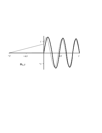
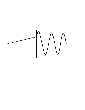
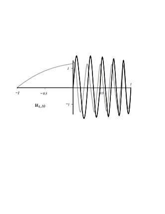
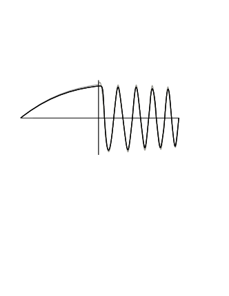
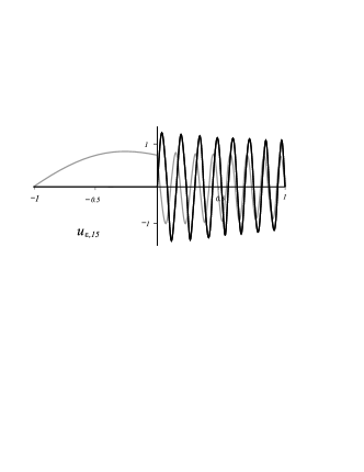
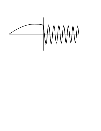
Figure 1: A comparison of the low and high frequency approximations (black plots) with the eigenfunctions (grey plots) for $u_{\varepsilon,5}$, $u_{\varepsilon,10}$ and $u_{\varepsilon,15}$ (from top to bottom).

Note that the method that is applied for the approximations in $1$–dimensional case is also applicable in a multidimensional situation. Nevertheless, the justification of it requires another technique, which is out of scope of this paper.

References

• [1] N. Babych, Yu. Golovaty, Quantized asymptotics of high frequency oscillations in high contrast media, Proc. of Waves 2007, (23-27 July 2007, University of Reading) p. 35–37.
• [2] G. P. Panasenko, Asymptotic behavior of the eigenvalues of elliptic equations with strongly varying coefficients, Trudy Sem. Petrovsk.,1987, vol.Β 12, 201–217.
• [3] M. Lobo-Hidalgo, E. SΓ‘nchez-Palencia, Low and high frequency vibration in stiff problems. Partial differential equations and the calculus of variations, Vol.Β II, 729–742, Progr. Nonlinear Differential Equations Appl., 2, Birkh user Boston, Boston, MA, 1989.
• [4] M. Lobo, E. M. PΓ©rez, High frequency vibrations in a stiff problem. Math. Models Methods Appl. Sci. 7 (1997), no. 2, 291–311.
• [5] Yu. Golovaty , N. Babych, On WKB asymptotic expansions of high frequency vibrations in stiff problems, in Proceedings of the Conference Equadiff ’99, Berlin 1999. Singapore: World Scientific. Vol. 1: 103–105, 2000.
• [6] J. Sanchez Hubert , E. Sanchez Palencia, Vibration and coupling of continuous systems. Asymptotic methods, Berlin etc.: Springer-Verlag. xv, 1989.
• [7] N. Babych, Yu. Golovaty, Asymptotic analysis of vibrating system containing stiff-heavy and flexible-light parts. Preprint of Bath Institute For Complex Systems, Bath 2007. On-line: www.bath.ac.uk/math-sci/bics/preprints
• [8] Yu. D. Golovaty, D. Gomez, M. Lobo and E. Perez, Asymptotics for the eigenelements of vibrating membranes with very heavy thin inclusions. C.R. Mecanique, 330 (11) 2002, 777–782.
• [9] Yu. D. Golovaty, D. Gomez, M. Lobo and E. Perez, On vibrating membranes with very heavy thin inclusions, Mathematical Models & Methods in Applied Sciences, Vol. 14, No.7 (2004) 987–1034.
• [10] D. Gomez, M. Lobo, S. Nazarov, E. Perez, Spectral stiff problems in domains surrounded by thin bands: Asymptotic and uniform estimates for eigenvalues, J. Math. Pures Appl. 85 (2006), 598–632.
• [11] E. PΓ©rez, On the whispering gallery modes on the interfaces of membranes composed of two materials with very different densities, Math. Mod. Meth. Appl. Sci. 13 (2003), 75–98.
• [12] N. Babych, I. Kamotski, V. Smyshlyaev, Homogenization in periodic media with doubly high contrasts, arXiv:0711.2405v1.
• [13] T. Kato, Perturbation theory for linear operators. Die Grundlehren der mathematischen Wissenschaften, Band 132. Springer-Verlag New York, Inc., New York, 1966.
• [14] M. I. Vishik, L. A. Lyusternik, Regular degeneration and boundary layer for linear differential equations with small parameter, Uspehi Mat. Nauk (N.S.), Vol. 12, no. 5(77), 1957, 3–122.
• [15] M.Β V.Β Fedoryuk, Asymptotic analysis. Linear ordinary differential equations, Berlin: Springer-Verlag, 1993.