SLE local martingales in logarithmic representations

Abstract

A space of local martingales of SLE type growth processes forms a representation of Virasoro algebra, but apart from a few simplest cases not much is known about this representation. The purpose of this article is to exhibit examples of representations where $L_{0}$ is not diagonalizable — a phenomenon characteristic of logarithmic conformal field theory. Furthermore, we observe that the local martingales bear a close relation with the fusion product of the boundary changing fields.

Our examples reproduce first of all many familiar logarithmic representations at certain rational values of the central charge. In particular we discuss the case of SLE_κ=6 describing the exploration path in critical percolation, and its relation with the question of operator content of the appropriate conformal field theory of zero central charge. In this case one encounters logarithms in a probabilistically transparent way, through conditioning on a crossing event. But we also observe that some quite natural SLE variants exhibit logarithmic behavior at all values of $\kappa$, thus at all central charges and not only at specific rational values.

Kalle Kytölä

kalle.kytola@math.unige.ch

Section de math matiques, Universit de Gen ve

2-4 Rue du Li vre, CP 64, 1211 Gen ve 4, Switzerland.

1 Introduction

Conformal invariance is without a doubt one of the most powerful concepts in the research of two dimensional critical phenomena. When the microscopic lengthscale provided by a lattice is taken to zero in a model of statistical mechanics at its critical point, the scaling limit is expected to be conformally invariant in a suitable sense. If the scaling limit is understood in terms of a quantum field theory, one speaks of conformal field theory (CFT) [BPZ84, DFMS97]. Applying conformal field theory to statistical mechanics has lead to numerous great successes since 1980’s — some of the most fundamental and best established results concern exact values of critical exponents, correlation functions and partition functions (in particular modular invariant ones on the torus).

The way the conformal invariance assumption is exploited in conformal field theories is through the effect that infinitesimal local conformal transformations have on correlation functions of local fields. The (central extension of the) Lie algebra of these infinitesimal transformations is the Virasoro algebra, and it seems fair to say that the representation theory of Virasoro algebra forms the basis of all conformal field theory. In particular, conformal field theories built from a finite number of irreducible highest weight representations, the so called minimal models, were able to explain critical exponents in many of the most important two dimensional models of statistical physics.

It is nevertheless worth noting that in some applications of conformal field theory, minimal models were found insufficient. Among notable examples were percolation and polymers of different kinds [Sal87, SR93, Car99]. These cases often required something called logarithmic conformal field theory (LCFT) — the assumption that had to be relaxed from representation theory point of view was that of diagonalizability of $L_{0}$, the Virasoro generator corresponding physically to energy [Gur93].

Since almost a decade now, the conformal invariance assumption has been exploited also in another, rather different way. The introduction of Schramm-Loewner evolutions (SLE) [Sch00] marked the starting point in the study of random curves whose probability distribution was postulated to be conformally invariant. Supplemented with another natural assumption from statistical physics, the requirement of conformal invariance of the probability distribution is powerful enough to identify the possible random curves up to one free parameter $\kappa>0$ — resulting in what is known as SLE_κ. More accurately, this is true when one chooses boundary conditions conveniently, whereas more general boundary conditions require introducing variants of SLEs. The approach has been very fruitful for making rigorous connection with lattice models of statistical mechanics. It has been proven in several cases that the law of an interface in a critical lattice model converges to SLE as the lattice spacing is taken to zero.

When it comes to the necessary mathematical techniques, these new methods differ significantly from conformal field theories. The very definition of SLEs does use a complex analysis technique of Loewner chains [Loe23] essentially composing infinitesimal conformal maps to describe the curve as a growth process. But to answer questions about the random curves, calculations mostly involve Itô’s stochastic analysis: a crucial step in solving an SLE problem is often that of finding an appropriate martingale.

Despite the differences of the paradigms of conformal field theory and Schramm-Loewner evolutions, there is an increasing amount of overlap. The purpose of the present article is to continue building a bridge between the two. The particular example of an interplay of SLE and CFT concepts relevant to us is the observation that local martingales of the SLE growth processes carry a representation of the Virasoro algebra [Kyt07]. We will study this representation in some detail, and in doing so show the relevance to SLEs of yet other conformal field theory concepts: the above mentioned logarithmic conformal field theories, and fusion products. Concretely, in Sections 3 and 4 we will examine explicitly for several variants of SLE the structure of the Virasoro representation consisting of local martingales. We will in particular find examples where $L_{0}$ is not diagonalizable. The results suggest a very close relationship between the local martingales and the fusion product of the boundary condition changing fields of the variant. More precisely, in all the examples we observe that the contragredient of the fusion product can be realized as local martingales.

In parallel with finding the structure of the Virasoro module of local martingales and comparing it with fusion products from CFT literature, we attempt to interpret clearly in probabilistic terms the different SLE variants used. Particularly the case of critical percolation is well suited for both purposes, so we devote the whole Section 4 to this. On one hand SLE is known rigorously to describe the scaling limit of the exploration path in percolation [Smi01, CN07], while on the other hand the question of the precise nature of the CFT of percolation has attracted a lot of attention recently [MR07, RP07, RS07, EF06]. Despite definite successes such as the Cardy’s crossing probability formula [Car92], fundamental questions about the conformal field theory appropriate for percolation have remained unsettled, notably that of the operator content of the theory. In rough terms the operator content of a CFT should be a class of representations (the fields of the theory) closed under the fusion product. We will reproduce as local martingales a few of the most fundamental fusions starting from the Cardy’s boundary changing field. Furthermore, we observe that the simplest fusion that produces logarithmic representation appears in an SLE variant that has a transparent probabilistic meaning: it is obtained by conditioning on a crossing event. After such confirmations of the emerging picture of the operator content of percolation [MR07], we speculate in Section 4.5 whether SLEs can be used to test another recent argument: the claimed inconsistency of adding certain other operators to the theory [MR08].

The present exercise has a few byproducts perhaps of direct interest to logarithmic conformal field theory. Most obviously, contrary to the common situation in LCFT literature where logarithms appear at specific rational values of the central charge, our logarithmic representations for SLEs cover the entire range $\infty<c\leq 1$. Section 3.4 also shows how extremely easy calculations give the values of logarithmic couplings, and these results agree with and extend a particular case of a recent proposal [MR08] made in the context of logarithmic minimal models. It is also possible that our rather straighforward setup may lend to development of alternative computational methods to study fusion in CFTs.

We finish this introduction by briefly mentioning other works relating SLEs and logarithmic conformal field theory. While a coherent theory of such a relation is yet to be discovered, the question has already been investigated with a few different approaches. The first articles discussing SLE and LCFT in parallel seem to be [Ras04, MARR04]. More recently [SAPR09] studied geometric questions in lattice loop models that bear a relation to both logarithmic minimal models and SLEs, and [CS08] used correlation functions of LCFT among other things to provide a formula for the probability of an SLE event involving a global geometric configuration of curves. A study of closed operator algebras [MR08] of LCFTs also exhibits a duality somewhat suggestive of SLEs. Despite the fact that these few attempts start from very different points of view, they all seem to point towards the conclusion that the approapriate conformal field theory description of SLEs is logarithmic. In hindsight we may observe that many of the statistical models that originally required abandoning minimal models in favor of logarithmic conformal field theory were of geometric nature [Sal87, Car99]: polymers themselves or percolation clusters are objects whose global spatial configuration is the natural object of interest. In fact [SAPR09] seems to suggest as some sort of rule of thumb that treating questions of global geometric kind, rather that just correlations of local degrees of freedom at a distance, typically requires logarithms in the CFT description [SAPR09].

2 Preliminaries

The aim is to make this paper readable for different audiences, in particular knowledge of either SLE or CFT alone should suffice. For this reason it is necessary to cover briefly a variety of topics in this background section. Below are some suggestions about accessible literature for each of the topics covered. This section also serves to fix notations.

Section 2.1 is devoted to a brief account on Schramm-Loewner evolutions (SLE), in particular variants known as SLE${}_{\kappa}(\rho)$. The books and reviews [Wer04, Law05, BB06, KN04] serve as comprehensive treatments of the topic and contain references to research articles. The Virasoro algebra and the kinds of representations that will be needed later on are discussed in Section 2.2. Classical results stated there can be found in e.g. [Ast97], whereas the more exotic staggered Virasoro modules are treated in detail in [KR09]. Finally, Section 2.3 reminds in which sense local martingales of the SLE growth process form a representation of Virasoro algebra, a result taken from [Kyt07].

2.1 Schramm-Loewner evolutions in the upper half plane

The random curves described by the SLE growth processes are characterized by two properties that make them suitable to describe curves in statistical mechanics at criticality. One, the domain Markov property, is a statement about the conditional probability law of the curve given an initial segment of it, and it is often very easy to verify for curves in statistical mechanics models. The other, conformal invariance, is a property that is argued to emerge in the scaling limit taken at the critical point. Roughly speaking these properties imply that the local behavior of the curve is characterized by one parameter, $\kappa>0$, while precise global statistics still depend on boundary conditions imposed. Since any two simply connected open domains (with at least two distinct boundary points) of the Riemann sphere are conformally equivalent, the conformal invariance property in particular allows us to work in a reference domain, which we take to be the upper half plane $\mathbb{H}=\{z\in\mathbb{C}:\Im\textrm{m }z>0\}$.

2.1.1 Chordal SLE_κ in the upper half plane

The simplest choice of boundary conditions is such that it merely ensures the existence of a curve from one boundary point of the domain to another. The corresponding SLE is known as the chordal SLE. To define the chordal SLE_κ in $\mathbb{H}$ from $0$ to $\infty$ consider the ordinary differential equation (Loewner’s equation)

$$\frac{\mathrm{d}}{\mathrm{d}t}g_{t}(z)\;=\; \frac{2}{g_{t}(z)-X_{t}}\textrm{ ,}$$ (1)

with initial condition $g_{0}(z)=z\in\mathbb{H}$. The driving process $(X_{t})_{t\in[0,\infty)}$ is taken to be $X_{t}=\sqrt{\kappa}\;B_{t}$, where $(B_{t})_{t\in[0,\infty)}$ is a standard normalized Brownian motion and $\kappa>0$. For each $z\in\mathbb{H}$, let $\tau_{z}$ be the maximal time up to which the solution to (1) exists with the initial condition $z$. The set $\mathbb{H}_{t}=\{z\in\mathbb{H}:\tau_{z}>t\}$, $t\geq 0$, is a simply connected open set and $g_{t}$ is the unique conformal map $\mathbb{H}_{t}\rightarrow\mathbb{H}$ with $g_{t}(z)=z+\mathcal{O}(z^{-1})$ as $z\rightarrow\infty$. We denote the Laurent expansion at infinity of $g_{t}$ by

$$g_{t}(z)=z+\sum_{m=2}^{\infty}a_{m}(t)\,z^{1-m}\textrm{ .}$$ (2)

It can be shown that in this setup the Loewner’s equation (1) specifies a non self-crossing curve $\gamma:[0,\infty)\rightarrow\overline{\mathbb{H}}$ such that $\mathbb{H}_{t}$ is the unbounded component of $\mathbb{H}\setminus\gamma[0,t]$, see [RS05]. The curve $\gamma$ is called the trace of the chordal SLE_κ (in $\mathbb{H}$ from $0$ to $\infty$). For $\kappa\leq 4$ it is a simple curve (non-self intersecting), for $\kappa>4$ it has self-intersections, and for $\kappa\geq 8$ it visits every point of the domain [RS05].

For several lattice models of statistical physics, with appropriate boundary conditions to account for a chordal curve, the continuum limit of the law of a curve has been shown to be chordal SLE_κ — the value of $\kappa$ depends on the particular model. For yet many others, similar results are conjectured. In Section 4 we will make the most explicit comparisons with the CFT literature on percolation, which corresponds to $\kappa=6$. The precise description of the continuum limit result in this case will be given in Section 4.1.

2.1.2 SLE${}_{\kappa}(\rho)$ in the upper half plane

While for many lattice models it is possible to find boundary conditions such that the chordal SLE is the correct scaling limit, this is by no means the general case. To account for somewhat more general boundary conditions, we take the driving process $(X_{t})$ to be a solution to the Itô stochastic differential equation

$$\mathrm{d}X_{t}\;=\; \sqrt{\kappa}\;\mathrm{d}B_{t}+\kappa\big{(}\frac{\partial}{\partial x}\log Z(X_{t},g_{t}(Y_{0}))\big{)}\;\mathrm{d}t\textrm{ ,}$$ (3)

where $(B_{t})_{t\geq 0}$ is standard Brownian motion and $Z(x,y)=(x-y)^{\rho/\kappa}$ is what we call the partition function. The processes are defined on a random time interval $t\in[0,\tau)$, where $\tau$ is a stopping time. The resulting process is known as SLE${}_{\kappa}(\rho)$, and it is a variant of SLE in the sense that the probability measure is absolutely continuous with respect to the chordal SLE_κ when restricted to the curve up to times smaller than $\tau$. One could allow more general variants by letting the partition function $Z$ depend on more points, e.g. [Kyt07]. Although mostly SLE${}_{\kappa}(\rho)$ is enough for us, we will once in Section 4.5 replace the $Z$ above by $Z(x,y_{1},y_{2})=(x-y_{1})^{\rho_{1}/\kappa}(x-y_{2})^{\rho_{2}/\kappa}(y_{1}-y_{2})^{\rho_{1}\rho_{2}/2\kappa}$, and get a variant which we call SLE${}_{\kappa}(\rho_{1},\rho_{2})$. In the rest of the article we denote briefly $g_{t}(Y_{0})=:Y_{t}$.

2.1.3 Examples of SLE${}_{\kappa}(\rho)$

Without even considering lattice models, it is easy to see that the generalization SLE${}_{\kappa}(\rho)$ is useful. As an obvious remark we note that with $\rho=0$ the partition function is constant $Z(x,y)=1$, thus $\frac{\partial}{\partial x}\log Z=0$, and SLE${}_{\kappa}(\rho=0)$ is nothing but the chordal SLE. Below we will give two more interesting examples of SLE${}_{\kappa}(\rho)$, which will also facilitate giving probabilistic interpretations in later sections.

First, take the chordal SLE_κ, for $\kappa>4$, and imagine conditioning it on the event that the curve doesn’t touch the interval $[Y_{0},\infty)$, a situation that has been considered e.g. in [Dub05]. Equivalently, the difference of the $X$ and $Y$ processes, $D_{t}=Y_{t}-X_{t}$, shouldn’t hit zero. The process $D_{t}$ is a linear time change of Bessell process of dimension $d=\frac{4+\kappa}{\kappa}$. One easily computes by Itô’s formula that starting from $D_{0}$, the probability that $|D_{t}|>0$ for all $t\in[0,T]$ is $\mathsf{P}\big{[}|D_{t}|>0\textrm{ for }0\leq t\leq T\big{]}\,=\,G(|D_{0}|/\sqrt{T})$, where

$$G(r)\;=\;\frac{\int_{0}^{r}s^{1-d}e^{-\frac{1}{2\kappa}s^{2}}\;\mathrm{d}s}{\int_{0}^{\infty}s^{1-d}e^{-\frac{1}{2\kappa}s^{2}}\;\mathrm{d}s}\textrm{ .}$$

Under the conditioned probability measure $\mathsf{P}\big{[}\;\cdot\;\big{|}|D_{t}|>0\textrm{ for }t\in[0,T]\big{]}$, the driving process $X_{t}$ satisfies by Girsanov’s formula

$$\mathrm{d}X_{t}\;=\;\sqrt{\kappa}\;\mathrm{d}B^{\prime}_{t}+\kappa\;\Big{(}\frac{\partial}{\partial D}\;\log G\big{(}\frac{|D_{t}|}{\sqrt{T}}\big{)}\Big{)}\;\mathrm{d}t$$

where $B^{\prime}$ is a standard Brownian motion under the conditioned measure. Taking $T\rightarrow\infty$, this tends to

$$\mathrm{d}X_{t}\;=\;\sqrt{\kappa}\;\mathrm{d}B^{\prime}_{t}+\frac{\kappa-4}{X_{t}-Y_{t}}\;\mathrm{d}t$$

which is the driving process of SLE${}_{\kappa}(\rho)$ with $\rho=\kappa-4$. Thus indeed a simple conditioning of the chordal SLE_κ leads to an SLE${}_{\kappa}(\rho)$.

As the second example, we will consider coordinate changes. Suppose we take an SLE${}_{\kappa}(\rho^{\prime})$ in $\mathbb{H}$ (in particular $\rho^{\prime}=0$ corresponds to the chordal SLE) and consider a Möbius image of the curve. More precisely, take $\mu:\mathbb{H}\rightarrow\mathbb{H}$ a Möbius transformation of the half plane such that $\mu(X_{0})=\tilde{X}_{0}\in\mathbb{R}$, $\mu(Y_{0})=\infty$ and $\mu(\infty)=\tilde{Y}_{0}\in\mathbb{R}$. Then consider the curve $\tilde{\gamma}=\mu(\gamma)$ as an unparametrized but oriented curve starting from $\tilde{X}_{0}$. A standard computation (see e.g. [SW05]) shows that the law of $\tilde{\gamma}$ is SLE${}_{\kappa}(\rho=\kappa-6-\rho^{\prime})$. For example the chordal SLE_κ in $\mathbb{H}$ whose target point is $Y_{0}$ instead of $\infty$ is obtained as the above Möbius image (because of the conformal invariance property), therefore it is an SLE${}_{\kappa}(\rho=\kappa-6)$. We could also coordinate change the first example $\rho^{\prime}=\kappa-4$. A chordal SLE_κ from $X_{0}$ to $Y_{0}$ conditioned not to touch $(Y_{0},\infty]$ is then seen to be an SLE${}_{\kappa}(\rho=-2)$. Interestingly for the purpose of the present paper, this last example will always exhibit logarithms as will be shown in Section 3.3.

2.2 Virasoro algebra and its representations

The Virasoro algebra $\mathfrak{vir}$ is the complex Lie algebra spanned by $L_{n}$, $n\in\mathbb{Z}$ and $C$ with commutation relations

$$[L_{n},L_{m}]\;=\;(n-m)\;L_{n+m}+\frac{n^{3}-n}{12}\delta_{n+m,0}\;C\quad,\qquad[C,L_{n}]\;=\;0\textrm{ .}$$

In a conformal field theory the central charge $c$ is a number characteristic of the theory such that $C$ acts as $c\,\mathbf{1}$ in all the representations. We will only consider such representations and the value of $c$ is determined by $\kappa$ via $c(\kappa)=13-6\,\frac{\kappa}{4}-6\,\frac{4}{\kappa}$. Let $\mathcal{U}$ denote the universal enveloping algebra of $\mathfrak{vir}$ modulo the identification of $C=c\mathbf{1}$ and $\mathcal{U}^{\pm}$ the universal enveloping algebras of the Lie subalgebras $\mathfrak{vir}^{\pm}$ generated by $L_{n}$ with $\pm n>0$. These are graded by $\mathcal{U}=\oplus_{m\in\mathbb{Z}}\;\mathcal{U}_{m}$, where the homogeneous component $\mathcal{U}_{m}$ is has a Poincaré-Birkhoff-Witt basis consisting of $\cdots L_{-2}^{k_{-2}}\,L_{-1}^{k_{-1}}\,L_{0}^{k_{0}}\,L_{1}^{k_{1}}\,L_{2}^{k_{2}}\cdots$ with $\sum_{n\in\mathbb{Z}}nk_{n}=-m$, and similarly for $\mathcal{U}^{\pm}$.

We fix some notation and discuss the class of representations we will consider. For a $\mathfrak{vir}$ module $\mathcal{M}$, let $\mathcal{M}_{[\eta]}$ be the subspace consisting of those $u\in\mathcal{M}$ for which $(L_{0}-\eta)^{N}u=0$ for $N$ large enough. We call $\mathcal{M}_{[\eta]}$ the generalized eigenspace of eigenvalue $\eta$.

The representations we will study can be written as direct sums of finite dimensional generalized $L_{0}$ eigenspaces, with eigenvalues bounded from below. In indecomposable representations the generalized eigenvalues can only differ by integers, so denoting by $h$ the lowest $L_{0}$ eigenvalue and by $\mathcal{M}_{m}=\mathcal{M}_{[h+m]}$ we have $\mathcal{M}=\oplus_{m=0}^{\infty}\,\mathcal{M}_{m}$. We call $\mathcal{M}_{m}$ the grade $m$ of $\mathcal{M}$. Note that $L_{n}$, or indeed any $U\in\mathcal{U}_{-n}$, maps $\mathcal{M}_{m}$ to $\mathcal{M}_{m-n}$. To any such module $\mathcal{M}$ we can associate the contragredient module $\mathcal{M}^{*}$ as follows. Let $\mathcal{M}_{n}^{*}$ be the vector space dual of the finite dimensional space $\mathcal{M}_{n}$ and define $\mathcal{M}^{*}=\oplus_{n=0}^{\infty}\mathcal{M}_{n}^{*}$, with Virasoro action given by $\big{<}L_{n}\,v^{*},v\big{>}=\big{<}v^{*},L_{-n}\,v\big{>}$. To facilitate a similar formula with the universal enveloping algebra the anti-involution $\dagger$ is defined by linear extension of $(L_{n_{1}}\cdots L_{n_{k}})^{\dagger}\,=\,L_{-n_{k}}\cdots L_{-n_{1}}$, so that $\big{<}U^{\dagger}\,v^{*},v\big{>}=\big{<}v^{*},U\,v\big{>}$ for all $U\in\mathcal{U}$, $v\in\mathcal{M}$, $v^{*}\in\mathcal{M}^{*}$.

2.2.1 Highest weight representations

The most important representations for conformal field theory are highest weight representations. A $\mathfrak{vir}$ module $\mathcal{H}$ is called a highest weight representation of highest weight $h\in\mathbb{C}$ if there exists a non-zero $w\in\mathcal{H}$, called a highest weight vector, such that $L_{0}\,w=h\,w$, $L_{n}\,w=0$ for all $n>0$ and $\mathcal{H}=\mathcal{U}\,w$. There is a universally repelling object in the category of highest weight modules of fixed $c$ and $h$, the Verma module with highest weight vector $v_{c,h}$

$$\mathcal{V}_{c,h}\;=\;\bigoplus_{\begin{subarray}{c}k\in\mathbb{N}\\ 0<n_{1}\leq n_{2}\leq\cdots\leq n_{k}\end{subarray}}\mathbb{C}\;L_{-n_{k}}\cdots L_{-n_{1}}\;v_{c,h}\textrm{ .}$$

The universal property guarantees that for any highest weight module $\mathcal{H}$ with a highest weight vector $w$ there exists a unique surjective $\mathfrak{vir}$-homomorphism $\mathcal{V}_{c,h}\rightarrow\mathcal{H}$ such that $v_{c,h}\mapsto w$. Therefore any highest weight module is a quotient of the Verma module by a submodule.

The submodule structure of Verma modules was resolved by Feigin and Fuchs [FF83, FF84], see also [FF90, Ast97]. We will state the result below, emphasizing the differences in the cases when $\kappa$ is rational or not. Recall first that $c$ is parametrized as $c=c(\kappa)=13-6\frac{\kappa}{4}-6\frac{4}{\kappa}$. In addition we define $h_{r,s}(\kappa)=\frac{\kappa/4}{4}(r^{2}-1)-\frac{1}{2}(rs-1)+\frac{4/\kappa}{4}(s^{2}-1)$. We point out that this parametrization has the symmetries $h_{-r,-s}=h_{r,s}$ and $h_{r+a,s+a\kappa/4}=h_{r,s}$ for any $a$, and also note that $h_{r,s}+rs=h_{r,-s}$.

The most important thing about the submodules of the Verma module $\mathcal{V}_{c(\kappa),h}$ is that any submodule is generated by singular vectors, eigenvectors $w^{\prime}$ of $L_{0}$ which are annihilated by the positive generators, $L_{n}w^{\prime}=0$ for $n>0$ (such a vector generates a highest weight submodule). Furthermore, up to multiplicative scalar there is never more than one singular vector at a given grade. It can be shown that there are no other singular vectors than those proportional to the highest weight vector $v_{c,h}$ in the Verma module $\mathcal{V}_{c(\kappa),h}$ unless $h=h_{r,s}(\kappa)$ for some $r,s\in\mathbb{Z}_{+}$. In other words, $\mathcal{V}_{c(\kappa),h}$ can only be reducible if $h=h_{r,s}(\kappa)$. We will describe these reducible cases below and in and the Figure 1, where the dots represent singular vectors and an arrow from one dot to another signifies the fact that the latter is contained in the submodule generated by the former.

Irrational $\kappa$: Suppose $\kappa\notin\mathbb{Q}$ and $h=h_{r,s}(\kappa)$ for some $r,s\in\mathbb{Z}_{+}$. The choice of such $r,s$ is unique when $\kappa$ is not rational. Then there is a singular vector $w^{\prime}$ in $\mathcal{V}_{c(\kappa),h}$ at grade $rs$. The submodule generated by $w^{\prime}$ is the maximal proper submodule of $\mathcal{V}_{c(\kappa),h}$ and is itself an irreducible Verma module, $\mathcal{U}w^{\prime}\cong\mathcal{V}_{c(\kappa),h+rs}$.

Rational $\kappa$: Suppose $\kappa=4\frac{p}{q}$ with $p,q\in\mathbb{Z}_{+}$ relatively prime. Suppose furthermore that $h=h_{r,s}(\kappa)$ for some $r,s\in\mathbb{Z}_{+}$. It is convenient to to take $r^{\prime},s^{\prime}$ such that $h=h_{r^{\prime},s^{\prime}}(\kappa)=h_{r,s}(\kappa)$ and the product $r^{\prime}s^{\prime}>0$ is minimal. There are still two structural possibilities that we name "braid" and "chain" following the terminology introduced in [KR09].

Assume that $q\nmid r$ and $p\nmid s$, a case that we will call braid. Then we choose also $r^{\prime\prime},s^{\prime\prime}\in\mathbb{Z}_{+}$ such that $h=h_{r,s}(\kappa)=h_{r^{\prime\prime},s^{\prime\prime}}(\kappa)$ and $r^{\prime\prime}s^{\prime\prime}>r^{\prime}s^{\prime}$ is minimal among the remaining choices. The Verma module $\mathcal{V}_{c(\kappa),h}$ contains singular vectors $w^{\prime}$ at grade $r^{\prime}s^{\prime}$ and $w^{\prime\prime}$ at grade $r^{\prime\prime}s^{\prime\prime}$ and the maximal proper submodule is generated by these. The highest weight submodules generated by these singular vectors are themselves braid type Verma modules $\mathcal{U}w^{\prime}\cong\mathcal{V}_{c(\kappa),h+r^{\prime}s^{\prime}}$ and $\mathcal{U}w^{\prime\prime}\cong\mathcal{V}_{c(\kappa),h+r^{\prime\prime}s^{\prime\prime}}$. The intersection $\mathcal{U}w^{\prime}\cap\mathcal{U}w^{\prime\prime}$ is the maximal proper submodule in both $\mathcal{U}w^{\prime}$and $\mathcal{U}w^{\prime\prime}$.

The other possibility, $q\mid r$ or $p\mid s$, will be called chain. There is a singular vector $w^{\prime}$ at grade $r^{\prime}s^{\prime}$ and $\mathcal{U}w^{\prime}$ is the maximal proper submodule of $\mathcal{V}_{c(\kappa),h}$. This submodule is itself a chain type Verma module, $\mathcal{U}w^{\prime}\cong\mathcal{V}_{c(\kappa),h+r^{\prime}s^{\prime}}$.

Figure 1: Submodule structure of Verma modules.

We adopt a few notational conventions for highest weight modules. Verma modules $\mathcal{V}_{c,h}$ were already considered above. Other highest weight modules are quotients of the Verma modules. In pictures we use the convention that a black (filled) dot represents a non-zero singular vector whereas a white (empty) dot represents a singular vector that is quotiented away from the Verma module (we sometimes refer to this as a null vector). Arrows still represent inclusions between the submodules generated by the singular vectors. We denote by $\mathcal{Q}_{\kappa;r,s}$ the highest weight module that is the quotient of $\mathcal{V}_{c(\kappa),h_{r,s}(\kappa)}$ by the submodule generated by singular vector at level $rs$, and by $w_{\kappa;r,s}$ the highest weight vector in $\mathcal{Q}_{\kappa;r,s}$. In general $\mathcal{Q}_{\kappa;r,s}$ need not be irreducible (it is only if $\kappa\notin\mathbb{Q}$ or if in the chain case $rs>0$ is minimal). We denote the irreducible highest weight module obtained as the quotient of $\mathcal{V}_{c,h}$ by its maximal proper submodule by $\mathcal{L}_{c,h}$. For notational simplicity we also often omit explicit references to $\kappa$ and $c$.

2.2.2 Staggered modules

In logarithmic conformal field theories one encounters indecomposable representations more complicated than just highest weight representations. In particular, the property that is responsible for the logarithms in correlation functions is the non-diagonalizability of $L_{0}$ [Gur93]. For our purposes, staggered modules [Roh96, KR09] of the kind that we describe below will be enough. We remark that in Sections 3 – 4 we will study concretely constructed $\mathfrak{vir}$-modules, so it is not important for us to know beforehand when a module of certain structure exists. Instead it is important to know which information is sufficient to uniquely characterize the module. The results stated below can be found in [KR09], see also [Roh96].

Suppose $\mathcal{H}^{\mathrm{L}},\mathcal{H}^{\mathrm{R}}$ are two highest weight modules of the same central charge $c$ and highest weights $h^{\mathrm{L}},h^{\mathrm{R}}$ and highest weight vectors $w^{\mathrm{L}},w^{\mathrm{R}}$ respectively. We call $\mathcal{S}$ a staggered module with left module $\mathcal{H}^{\mathrm{L}}$ and right module $\mathcal{H}^{\mathrm{R}}$ if it contains the former as a submodule $\mathcal{H}^{\mathrm{L}}\subset\mathcal{S}$, its quotient by this submodule is the latter $\mathcal{S}/\mathcal{H}^{\mathrm{L}}\cong\mathcal{H}^{\mathrm{R}}$, and $L_{0}$ is not diagonalizable on $\mathcal{S}$. This may be summarized in the short exact sequence

$$0\longrightarrow\mathcal{H}^{\mathrm{L}}\overset{\iota}{\longrightarrow}\mathcal{S}\overset{\pi}{\longrightarrow}\mathcal{H}^{\mathrm{R}}\longrightarrow 0$$

in addition to which we have the requirement of non-diagonalizability of $L_{0}$.

The simplest case is when $h^{\mathrm{R}}=h^{\mathrm{L}}$. Then we set $\xi=\iota(w^{\mathrm{L}})$ and pick a representative $\eta\in\pi^{-1}(\mathbb{C}w^{\mathrm{R}})$ such that $(L_{0}-h^{\mathrm{R}})\eta=\xi$ (possible by non-diagonalizability of $L_{0}$). The structure of such a staggered module is determined by the mere knowledge of $\mathcal{H}^{\mathrm{L}}$ and $\mathcal{H}^{\mathrm{R}}$.

A more interesting case is if $h^{\mathrm{R}}=h^{\mathrm{L}}+\ell$ with $\ell\in\mathbb{Z}_{+}$. We can then choose $\xi=\iota(w^{\mathrm{L}})$ and $0\neq\eta\in\pi^{-1}(\mathbb{C}w^{\mathrm{R}})$ in the generalized $L_{0}$ eigenspace of eigenvalue $h^{\mathrm{R}}$. Denote $(L_{0}-h^{\mathrm{R}})\eta=\omega_{0}\in\iota(\mathcal{H}^{\mathrm{L}})$ and assume without loss of generality $\omega_{0}\neq 0$ (were this not possible, $L_{0}$ would have to be diagonalizable). For $n>0$ we have $L_{n}\omega_{0}=L_{n}(L_{0}-h^{\mathrm{R}})\eta=(L_{0}-h^{\mathrm{R}}+\eta)L_{n}\eta=0$, since $L_{n}\eta\in\mathcal{H}^{\mathrm{L}}_{\ell-n}$. What this means is that $\omega_{0}$ is a non-zero singular vector in $\iota(\mathcal{H}^{\mathrm{L}})$, and in particular $\ell$ must be a grade of a singular vector in the Verma module of highest weight $h^{\mathrm{L}}$. We can assume a choice of $\eta$ such that $\omega_{0}=\chi\xi$ where

$$\chi=L_{-1}^{\ell}+\sum_{\begin{subarray}{c}n_{1}\geq n_{2}\geq\cdots\geq n_{k}\geq 1\\ n_{1}>1\;,\;\sum_{j}n_{j}=\ell\end{subarray}}d_{n_{1},\ldots,n_{k}}\;L_{-n_{1}}\cdots L_{-n_{k}}\;\in\;\mathcal{U}^{-}_{\ell}\textrm{ .}$$

Unlike the case $h^{\mathrm{R}}=h^{\mathrm{L}}$, here the structure of the module is in general not yet determined by the knowledge of left and right modules $\mathcal{H}^{\mathrm{L}},\mathcal{H}^{\mathrm{R}}$. It can be shown that depending on the particular $\mathcal{H}^{\mathrm{L}},\mathcal{H}^{\mathrm{R}}$ the set of isomorphism classes of such staggered modules is an affine subspace (possibly empty) of a vector space of dimension at most two [KR09]. Below we will content ourselves to state what is enough to identify the modules in a case that suffices for the needs of this paper.

Suppose the highest weight of $\mathcal{H}^{\mathrm{L}}$ is $h^{\mathrm{L}}=h_{r,s}$ with $r,s\in\mathbb{Z}_{+}$ such that the grade $\ell=rs>0$ the minimal at which $\mathcal{H}^{\mathrm{L}}$ contains a nonzero singular vector. With the notation and normalizations as above, note that $\chi^{\dagger}\eta$ must be proportional to the highest weight vector of $\iota(\mathcal{H}^{\mathrm{L}})$, that is $\chi^{\dagger}\eta=\beta\xi$ for some $\beta\in\mathbb{C}$. This $\beta$ is invariant (independent of the choices made), and given $\mathcal{H}^{\mathrm{L}},\mathcal{H}^{\mathrm{R}}$ its value is enough to determine the structure of the staggered module $\mathcal{S}$. The value of $\beta$ is known also as logarithmic coupling.

2.3 The Virasoro module of SLE local martingales

We now briefly recall the result of [Kyt07] by which local martingales of the SLE growth process form a Virasoro module.

Let $c,h_{x},h_{y}\in\mathbb{C}$ be parameters. Consider independent formal variables $a_{2},a_{3},\ldots$. The differential operators on $\mathcal{F}=C^{\infty}(\{(x,y)\in\mathbb{R}^{2}:x\neq y\})[a_{2},a_{3},a_{4},\ldots]$ given below satisfy the commutation relations of the Virasoro algebra

$$L_{2}\;=\; -\frac{\partial}{\partial a_{2}}+\sum_{l\geq 4}\big{(}(l-3)a_{l-n}\big{)}\frac{\partial}{\partial a_{l}}$$

$$L_{1}\;=\; \sum_{l\geq 3}\big{(}(l-2)a_{l-1}\big{)}\frac{\partial}{\partial a_{l}}+\frac{\partial}{\partial x}+\frac{\partial}{\partial y}$$

$$L_{n}\;=\; \frac{1}{(n-2)!}\Big{[}\big{[}[\cdot\!\cdot\!\cdot[L_{2},\underbrace{L_{1}],\ldots],L_{1}\big{]},L_{1}}_{\textrm{$n-2$ times}}\Big{]}\quad\textrm{ for $n>2$}$$

$$L_{0}\;=\; \sum_{l\geq 2}la_{l}\frac{\partial}{\partial a_{l}}+x\frac{\partial}{\partial x}+y\frac{\partial}{\partial y}+h_{x}+h_{y}$$

$$L_{-1}\;=\; \sum_{l\geq 2}\Big{(}(l+2)a_{l+1}+\sum_{\begin{subarray}{c}m_{1},m_{2}\geq 2\\ m_{1}+m_{2}=l+1\end{subarray}}a_{m_{1}}a_{m_{2}}\Big{)}\frac{\partial}{\partial a_{l}}$$

$$\qquad+\big{(}x^{2}-3a_{2}\big{)}\frac{\partial}{\partial x}+\big{(}y^{2}-3a_{2}\big{)}\frac{\partial}{\partial y}+2xh_{x}+2yh_{y}$$

$$L_{-2}\;=\; \sum_{l\geq 2}\Big{(}(l+4)a_{l+2}-4a_{2}a_{l}+\sum_{\begin{subarray}{c}m_{1},m_{2}\geq 2\\ m_{1}+m_{2}=l+2\end{subarray}}3a_{m_{1}}a_{m_{2}}$$

$$\qquad\qquad\qquad+\sum_{\begin{subarray}{c}m_{1},m_{2},m_{3}\geq 2\\ m_{1}+m_{2}+m_{3}=l+2\end{subarray}}a_{m_{1}}a_{m_{2}}a_{m_{3}}\Big{)}\frac{\partial}{\partial a_{l}}$$

$$\qquad+\big{(}x^{3}-4xa_{2}-5a_{3}\big{)}\frac{\partial}{\partial x}+\big{(}y^{3}-4ya_{2}-5a_{3}\big{)}\frac{\partial}{\partial y}$$

$$\qquad+(3x^{2}-4a_{2})h_{x}+(3y^{2}-4a_{2})h_{y}-\frac{c}{2}a_{2}$$

$$L_{-n}\;=\; \frac{1}{(n-2)!}\Big{[}\underbrace{L_{-1},\big{[}L_{-1},[\ldots,[L_{-1}}_{\textrm{$n-2$ times}},L_{-2}]\cdot\!\cdot\cdot]\big{]}\Big{]}\quad\textrm{ for $n>2$.}$$

We remark that as Virasoro modules are graded by their $L_{0}$ eigenvalues, it is reasonable in view of the explicit expression above to consider the variables $x$ and $y$ having degree $1$ and the variable $a_{l}$ having degree $l\geq 2$. The homogeneity degree of a function $\varphi\in\mathcal{F}$ then simply differs from its $L_{0}$ eigenvalue by $h_{x}+h_{y}$.

Let $\varphi\in\mathcal{F}$ and consider the stochastic process $\varphi_{t}=\varphi(X_{t},Y_{t},a_{2}(t),a_{3}(t),\ldots)$ where $X_{t},Y_{t},a_{2}(t),a_{3}(t),\ldots$ are the processes for SLE${}_{\kappa}(\rho)$ as defined in Section 2.1. Then Itô’s formula says that

$$Z(X_{t},Y_{t})\;\mathrm{d}\big{(}\frac{\varphi_{t}}{Z(X_{t},Y_{t})}\big{)}=(\cdots)\;\mathrm{d}B_{t}+(A_{\kappa;\rho}\;\varphi)(X_{t},Y_{t},a_{2}(t),\ldots)\;\mathrm{d}t\textrm{ ,}$$

where $A_{\kappa;\rho}$ is the differential operator

$$A_{\kappa;\rho}\;=\; \frac{\kappa}{2}\;\frac{\partial^{2}}{\partial x^{2}}+\frac{2}{y-x}\;\frac{\partial}{\partial y}-\frac{\rho(\rho+4-\kappa)/(2\kappa)}{(y-x)^{2}}$$

$$\qquad+2\sum_{l\geq 2}\Big{(}\sum_{\begin{subarray}{c}0\leq m\leq l-2\\ 0\leq r\leq\lfloor\frac{l-2-m}{2}\rfloor\end{subarray}}x^{m}(-1)^{r}\frac{(m+r)!}{m!\;r!}\sum_{\begin{subarray}{c}k_{1},\ldots k_{r}\geq 2\\ \sum k_{j}=l-m-2\end{subarray}}a_{k_{1}}\cdots a_{k_{r}}\Big{)}\;\frac{\partial}{\partial a_{l}}$$

and $Z(x,y)=(x-y)^{\rho/\kappa}$. We call $\mathrm{Ker}\;A_{\kappa;\rho}\subset C^{\infty}(\{(x,y):x\neq y\})[a_{2},a_{3},a_{4},\ldots]$ the space of local martingales of SLE${}_{\kappa}(\rho)$, because for any $\varphi\in\mathrm{Ker}\;A_{\kappa;\rho}$, the process $\frac{\varphi_{t}}{Z(X_{t},Y_{t})}$ is a local martingale.

If $c=c(\kappa)=13-6\frac{\kappa}{4}-6\frac{4}{\kappa}$, $h_{x}=h_{1,2}(\kappa)=\frac{6-\kappa}{2\kappa}$ and $h_{y}=\frac{\rho(\rho+4-\kappa)}{4\kappa}$, then $[L_{n},A_{\kappa;\rho}]=q_{n}(x,a_{2},a_{3},\ldots)\;A_{\kappa;\rho}$, where $q_{n}$ is a polynomial multiplication operator. In particular the space of local martingales, $\mathrm{Ker}\;A_{\kappa;\rho}$, is a Virasoro module. From now on assume that $c,h_{x},h_{y}$ are fixed in this way.

The physical interpretation of the above representation is the action of local conformal transformations on the boundary changing field located at infinity. The key idea in finding the representation was the idea of an “SLE state” built by composing intertwining operators corresponding to all the boundary changes on the real axis, followed by an implementation of the conformal transformation [BB04, Kyt07]. One may therefore expect the representation to be closely related to the fusion product of the boundary condition changing fields, which is indeed what we will see in the examples.

In the rest of the paper we will study the structure of this Virasoro module of local martingales for different SLE variants. In all cases, the modules $\mathrm{Ker}\;A_{\kappa;\rho}$ turn out to be essentially contragredient to the fusion products of the boundary changing fields. In addition to giving the results about the module $\mathrm{Ker}\;A_{\kappa;\rho}$, we always attempt both to discuss what is known about the corresponding fusion, and to give a probabilistic interpretation of the SLE variant used.

Once the question is posed this way and the SLE variant in question fixed, the study of the representations has become a very concretely posed problem. Keeping in mind generalities from representation theory, one typically needs to answer explicit questions such as computing graded dimensions (characters), checking whether certain descendants of vectors vanish or belong to subrepresentations etc. Of course even these checks may soon become laborous. We have performed them with the help of a computer by implementing computations with Virasoro algebra and the explicit differential operators $L_{n}$ and $A_{\kappa;\rho}$ given above.

3 Example modules and appearance of logarithms

3.1 The module for chordal SLE_κ

Before starting to analyze the more complicated cases, it is worth taking a look at the simplest and already well understood case, the chordal SLE_κ. This doesn’t yet involve fusions because the only boundary changing field on real axis is at the starting point of the curve. However even this simple case is quite interesting: for example in the case $\kappa=6$ discussed in Section 4, we will find a representation contragredient to the conformal family of the field $\psi$ Cardy used in deriving his famous crossing probability formula.

In the case of chordal SLE_κ, the partition function should be thought of as a constant $Z=1$. The space of local martingales, that is the kernel of

$$A_{\kappa}\;=\;\frac{\kappa}{2}\;\frac{\partial^{2}}{\partial x^{2}}+2\sum_{l\geq 2}\Big{(}\sum_{\begin{subarray}{c}0\leq m\leq l-2\\ 0\leq r\leq\lfloor\frac{l-2-m}{2}\rfloor\end{subarray}}\frac{x^{m}(-1)^{r}(m+r)!}{m!\;r!}\sum_{\begin{subarray}{c}k_{1},\ldots k_{r}\geq 2\\ \sum k_{j}=l-m-2\end{subarray}}a_{k_{1}}\cdots a_{k_{r}}\Big{)}\;\frac{\partial}{\partial a_{l}}\textrm{ ,}$$

has been studied in [BB03]. The differential operator $A_{\kappa}$ preserves the space $\mathcal{F}^{\mathrm{polyn.}}=\mathbb{C}[x,a_{2},a_{3},a_{4},\ldots]$ of polynomials. A clever argument allowed Bauer and Bernard to show that $A_{\kappa}$ maps $\mathcal{F}^{\mathrm{polyn.}}_{m}$ surjectively to $\mathcal{F}^{\mathrm{polyn.}}_{m-2}$, where the homogeneous subspaces are defined as before by $L_{0}$ eigenvalues. Combined with the observation

$$\mathrm{dim}\;\mathcal{F}^{\mathrm{polyn.}}_{m}\;=p(m)\;:=\; \#\{(k_{1},\ldots,k_{m})\in\mathbb{N}^{m}\;:\;\sum_{j}jk_{j}=m\}\textrm{ ,}$$

the surjectivity shows that the graded dimension of $\mathrm{Ker}\;A_{\kappa}\subset\mathcal{F}^{\mathrm{polyn.}}$ coincides with that of $\mathcal{Q}_{\kappa;1,2}$, namely $\mathrm{dim}\;(\mathrm{Ker}\;A_{\kappa})_{m}=p(m)-p(m-2)$. Better yet, a concrete construction [BB04] shows for any chordal SLE_κ that $\mathrm{Ker}\;A_{\kappa}$ is contragredient to the highest weight representation $\mathcal{Q}_{\kappa;1,2}$. The vectors of the lowest $L_{0}$ eigenvalue $h_{1,2}(\kappa)$ are constants, corresponding to the partition function of chordal SLE, $Z(x)=1$. This last remark relates to the trivial observation that $Z\in\mathrm{Ker}\;A_{\kappa;\rho}$, or the fact that constant processes are (local) martingales.

We will start by discussing the case of irrational $\kappa$ as it is the simplest in terms of representation theory. In this case $\mathcal{Q}_{\kappa;1,2}$ is the irreducible highest weight representation of highest weight $h=h_{1,2}(\kappa)=\frac{6-\kappa}{2\kappa}$. Now $\mathrm{Ker}\;A_{\kappa}\subset\mathcal{F}^{\mathrm{polyn.}}$ is also the irreducible $\mathcal{Q}_{\kappa;1,2}=\mathcal{L}_{h_{1,2}}$ with the partition function $Z=1$ as its highest weight vector, as can be seen directly from the graded dimension as in [BB03] or as follows from the fact that an irreducible highest weight representation is contragredient to itself. We emphasize that the situation will be different in the case of rational $\kappa$: when $\mathcal{Q}_{1,2}$ is a reducible highest weight representation, the contragredient $\mathcal{Q}_{1,2}^{*}$ is no longer a highest weight representation. The particular case of $\kappa=6$ will be made explicit in Section 4.2.

3.2 Naive fusions and the appearance of logarithms

The purpose of this paper is to exhibit logarithmic representations in the context of SLEs. The characteristic property of these representations is a nontrivial Jordan block structure of $L_{0}$. This is a degeneracy that can result from coincidence of conformal weights of several primary fields. This section is a discussion of how such coincidences appear in fusions.

While a proper definition of fusion product of representations is quite delicate [Gab94], there is also a somewhat naive, but very straightforward way of understanding fusion in CFT. This consists of saying that a primary field of conformal weight $h$ occurs in the fusion product of primary fields of weights $h^{\prime}$ and $h^{\prime\prime}$ if the three point function of these three fields is non-vanishing. Since three point functions are up to a multiplicative constant fixed by conformal invariance, the question boils down seeing whether a nonzero three point function satisfies all other requirements — notably the null field equations (differential equations that one gets via Ward identities [DFMS97]) if either of the fused fields has a vanishing descendant.

For concreteness, motivated by the physical understanding of the boundary changing fields for SLE let us consider naively the fusion of a field of weight $h_{1,2}=\frac{6-\kappa}{2\kappa}$ with a vanishing descendant at level two, and a field of weight $h(\rho)=\frac{1}{4\kappa}\rho(\rho+4-\kappa)$. The three point function of these two located at $x$ and $y$ with a field of weight $h$ at infinity would be proportional to $(x-y)^{h-h_{1,2}-h(\rho)}$. The appropriate null field equation relates immediately to SLE local martingales: it in fact reads $A_{\kappa;\rho}\,\big{(}(x-y)^{h-h_{1,2}-h(\rho)}\big{)}=0$. This boils down to the following equation for the conformal weights

$$\big{(}h-h_{1,2}-h(\rho)\big{)}\big{(}h-h_{1,2}-h(\rho)-1\big{)}+\frac{4}{\kappa}\big{(}h-h_{1,2}-h(\rho)\big{)}-\frac{4}{\kappa}h(\rho)\;=\;0\textrm{ .}$$ (4)

The two roots correspond naively to the two conformal weights that appear in the fusion

$$h^{+}\;=\; \frac{\rho^{2}+8\rho-\rho\kappa+12-2\kappa}{4\kappa}$$

$$h^{-}\;=\; \frac{\rho^{2}-\rho\kappa-4+2\kappa}{4\kappa}\textrm{.}$$

As a degenerate candidate for producing logarithmic representations, we might require the above two values to coincide, $h^{+}=h^{-}$. For any $\kappa$ we have a unique way of satisfying this, the choice $\rho=\frac{\kappa-4}{2}$. In Section 3.3 we will see that indeed the local martingales then form a simple staggered module, and later we’ll see that at $\kappa=8$ the representation becomes one very familiar from the physics literature.

But in fact the requirement of coincidence of $h^{\pm}$ is not the only way of getting coinciding weights for primary fields that arise in the fusion: a coincidence might happen also with some descendant field. In such a case we should have $h^{+}=h_{r,s}$ for some $r,s\in\mathbb{Z}_{+}$ and $h^{-}=h^{+}+\ell$ where $\ell\geq 0$ is the grade at which the $h^{+}$ module has a singular vector (or vice versa, the roles of $h^{\pm}$ exchanged). For $\kappa\notin\mathbb{Q}$, the only possibility is $\ell=rs$ and the desired values of $h^{\pm}$ can each be obtained by a choice of $\rho$

$$h^{+}=h_{r,s}\quad\Leftrightarrow\quad \rho\in\{\frac{\kappa r-4s+\kappa-8}{2},\frac{-\kappa r+4s+\kappa-8}{2}\}$$

$$h^{-}=h_{r,s}+rs\quad\Leftrightarrow\quad \rho\in\{\frac{\kappa r+4s+\kappa}{2},\frac{-\kappa r-4s+\kappa}{2}\}\textrm{ .}$$

For general $\kappa$ and $r,s$ the two requirements are in conflict with each other. But for $s=1$ and any $r$ we do obtain solutions at any $\kappa$, namely $\rho=-2+\frac{\kappa}{2}(1-r)$ (at specific values of $\kappa$ there may be also other solutions). We remark that requiring $h^{-}=h_{r,s}$, $h^{+}=h_{r,s}+rs$ instead merely correspods to changing $\rho$ to $\kappa-4-\rho$.

Apart from the above mentioned case $h^{+}=h^{-}$ we will consider two of the simplest examples of logarithmic representations that occur at generic values of $\kappa$. These are the cases $s=1$, $r=1,2$ above. In both cases there is a logarithmic coupling $\beta$ to be computed. In the first case of Section 3.4 the obtained value of $\beta$ will generalize a proposed infinite series of logarithmic couplings [MR08] to a continuum of representations here parametrized by $\kappa$. In the second case, Section 3.4.2, we obtain another formula very similar to such proposals and related conjectures (although no conjecture about this case had been presented). At rational values of $\kappa$ further computations are in principle needed to identify the precise structure of the representations we encounter. We will exemplify the phenomenon in Sections 3.6 and 4.4, and find again staggered modules familiar from the LCFT literature.

3.3 A simple calculation for the first staggered module

As discussed above, $\rho=\frac{\kappa-4}{2}$ might be a good place to start looking for logarithms. It is worth mentioning that this variant was used in the first globally precise formulation of a duality conjecture for SLEs [Dub05].

The partition function $Z\in\mathrm{Ker}\;A_{\kappa;\rho=(\kappa-4)/2}$ is explicitly

$$Z(x,y)\;=\;(x-y)^{\frac{\kappa-4}{2\kappa}}\textrm{ ,}$$

and corresponds to the constant (local) martingale. It is straightforward to verify with the formulas of Section 2.3 that

$$L_{n}Z=0\qquad\textrm{ for $n>0$, and }\qquad(L_{0}-\frac{8-\kappa}{16})Z=0\textrm{ ,}$$

so $Z$ generates a highest weight representation $\mathcal{U}Z\subset\mathrm{Ker}\;A_{\kappa;\rho=(\kappa-4)/2}$ of highest weight $h_{Z}=\frac{8-\kappa}{16}$. This weight coincides with $h_{Z}=h_{0,1}(\kappa)$. If $\kappa$ is rational the corresponding Verma module is reducible (chain type), but for $\kappa\notin\mathbb{Q}$ the Verma module is irreducible and we readily conclude that $\mathcal{U}Z\cong\mathcal{V}_{c(\kappa);h_{0,1}(\kappa)}$.

The naive fusion gave the weight $h_{Z}$ twice denenerate. This suggests we look not for another singular vector with $L_{0}$ eigenvalue $h_{Z}$, but instead for a “logarithmic partner to $Z$”, that is a function $\Lambda=\Lambda(x,y;a_{2},a_{3},\ldots)$ that forms an $L_{0}$ Jordan block with $Z$

$$(L_{0}-h_{Z})\Lambda=Z\textrm{ .}$$

Furthermore the requirement of it being annihilated by positive modes is in general expected to hold modulo the representation generated by $Z$. In this case homogeneity leaves us no other possibility but $L_{n}\Lambda=0$ for $n>0$ which in view of the explicit formulas for $L_{n}$ (Section 2.3) means that $\Lambda$ should not depend on $a_{k}$, $k\geq 2$, and should only be a function of the difference $x-y$. The obvious candidate

$$\Lambda(x,y)=(x-y)^{\frac{\kappa-4}{2\kappa}}\,\log(x-y)$$

satisfies not only the above properties, but most importantly $A_{\kappa;\rho}\Lambda=0$. In the language of stochastic processes, this is the property that

$$\frac{\Lambda(X_{t},Y_{t})}{Z(X_{t},Y_{t})}=\log(X_{t}-Y_{t})$$

is a local martingale for the growth process of $SLE_{\kappa}(\rho=\frac{\kappa-4}{2})$.

In view of the explicit properties above, we have the following observations about the structure of the representation $\mathcal{U}\Lambda\subset\mathrm{Ker}\;A_{\kappa;\rho=(\kappa-4)/2}$ generated by $\Lambda$. It is indecomposable and contains the highest weight module $\mathcal{U}Z$, because $(L_{0}-h_{Z})\,\Lambda=Z$. The quotient by $\mathcal{U}Z$ of this module is a highest weight module of highest weight $h_{Z}$, as follows from the facts that $(L_{0}-h_{Z})\Lambda,L_{1}\Lambda,L_{2}\Lambda\in\mathcal{U}Z$. Therefore $\mathcal{U}\Lambda$ is in any case a staggered module, with left and right modules having the same highest weight $h^{\mathrm{L}}=h^{\mathrm{R}}=h_{Z}$. At irrational $\kappa$ we readily conclude that the staggered module $\mathcal{U}\Lambda$ fits into the exact sequence

$$0\longrightarrow\mathcal{V}_{c(\kappa),h_{0,1}(\kappa)}\longrightarrow\mathcal{U}\Lambda\longrightarrow\mathcal{V}_{c(\kappa),h_{0,1}(\kappa)}\longrightarrow 0\textrm{ .}$$

From the general theory summarized in Section 2.2.2 we know that this is enough to identify the staggered module $\mathcal{U}\Lambda$.

3.4 Calculations for staggered modules with $h^{\mathrm{L}}\neq h^{\mathrm{R}}$

3.4.1 The simplest case

If the highest weights of the left and right module of a staggered module are different, the exact sequence alone is not enough to characterize the module (in general). The simplest such case is perhaps when the left module has weight $h_{1,1}=0$ and there is a logarithmic partner to a nonvanishing singular vector at grade one. In the discussion we identified $\rho=-2$ as the choice for which the naive fusion gives highest weights $h^{+}=0$ and $h^{-}=1$.

Indeed, the partition function

$$Z(x,y)=(x-y)^{-\frac{2}{\kappa}}$$

generates a highest weight representation $\mathcal{U}Z$ of highest weight $h_{Z}=0=h_{1,1}(\kappa)$ as follows once we check

$$L_{n}Z=0\qquad\textrm{ for $n>0$, and }\qquad(L_{0}-0)Z=0\textrm{ .}$$

Typically, a highest weight representation with $h=h_{1,1}=0$ in conformal field theory would only arise as the vacuum representation. While the Verma module has a singular vector at grade one, there are several arguments saying that there is none in the vacuum module: requirement of unitarity alone would suffice, but even relaxing that the translation invariance of the vacuum should imply the impossibility of grade one singular vector. But in logarithmic conformal field theory, the left modules of staggered modules must sometimes contain nonzero singular vectors, and indeed in the present case we compute that

$$L_{-1}Z\;=\;\frac{4-\kappa}{\kappa}\;(x-y)^{1-\frac{2}{\kappa}}$$

is such a nonzero (if $\kappa\neq 4$) singular vector, at grade one in $\mathcal{U}Z$. The $L_{0}$ eigenvalue of this singular vector, $h_{Z}+1=1$ was the other highest weight $h^{-}$ we got from the naive computation of fusion in Section 3.2. This again suggests looking for a logarithmic partner, now for $L_{-1}Z$. Let $\Lambda(x,y;a_{2},a_{3},\ldots)$ denote the function we are looking for. It should form a $L_{0}$ Jordan block with $L_{-1}Z$,

$$(L_{0}-1)\Lambda=L_{-1}Z$$

and positive modes acting on it should give something in the highest weight submodule $\mathcal{U}Z$. By considerations of grades, $L_{1}\Lambda\sim Z$ and $L_{n}\Lambda=0$ for $n\geq 2$. The latter implies no dependence on $a_{2},a_{3},\ldots$ again. A possible solution to all the equations so far would be

$$\frac{4-\kappa}{\kappa}\;(x-y)^{1-\frac{2}{\kappa}}\;\log(x-y)+b\;(x-y)^{-\frac{2}{\kappa}}\,(x+y)+a\;(x-y)^{1-\frac{2}{\kappa}}$$

although the last term, being already in $\mathcal{U}\,Z$ will affect none of our computations and can be omitted immediately. Now in general, dividing this by $Z$ will not give a local martingale of SLE${}_{\kappa}(\rho=-2)$ — we see that $A_{\kappa;\rho}\Lambda$ vanishes only if $b=\frac{4-\kappa}{8}$, so we define

$$\Lambda(x,y)=\frac{4-\kappa}{\kappa}(x-y)^{1-\frac{2}{\kappa}}\;\log(x-y)+\frac{4-\kappa}{8}\;(x-y)^{-\frac{2}{\kappa}}\,(x+y)\textrm{ .}$$

For irrational $\kappa$ the highest weight modules $\mathcal{U}Z$ and $\mathcal{U}\Lambda/\mathcal{U}Z$ of respective highest weights $0=h_{1,1}$ and $1=h_{1,-1}$ must both be Verma modules, so the staggered module $\mathcal{U}\Lambda\subset\mathrm{Ker}\;A_{\kappa;\rho=-2}$ has the exact sequence

$$0\longrightarrow\mathcal{V}_{c(\kappa),0}\longrightarrow\mathcal{U}\Lambda\longrightarrow\mathcal{V}_{c(\kappa),1}\longrightarrow 0\textrm{ .}$$

The invariant, logarithmic coupling, is then determined by computing $L_{1}\Lambda=(1-\frac{\kappa}{4})\,Z$, which gives $\beta=1-\frac{\kappa}{4}$.

It is interesting to compare with the study of a consistent operator algebra for logarithmic CFTs at central charges corresponding to $\kappa/4=\frac{p}{2}$, $p=3,5,7,\ldots$, [MR08]. In that article the authors propose an operator content of CFT, that would be closed under fusion products. Based on several computations of fusion products, the authors obtained that a staggered module with $h^{\mathrm{L}}=0$, $h^{\mathrm{R}}=1$ and our value $\beta=-\frac{p-2}{2}$ of the logarithmic coupling should be present for all $p$. Admittedly, at these rational values of $\kappa$ we haven’t yet determined the precise left and right modules, but the value of our invariant $\beta$ here provides both an interpolation and extrapolation of the proposal. Here it is moreover obtained by just a few lines of calculations instead of the use of a complicated algorithm [Gab94] needed to compute the structure of fusion product representations.

3.4.2 The next example in order of difficulty

Among the examples proposed in Section 3.2, $h^{+}=h_{r,1}$, the case $r=1$ considered above is a lot easier than the others. In order to show briefly that other cases are by no means untractable, we record the results of the next one here.

We take $\rho=\frac{-\kappa-4}{2}$, corresponding to $r=2$. The partition function $Z(x,y)=(x-y)^{-\frac{1}{2}-\frac{2}{\kappa}}$ generates a highest weight representation of weight $h_{Z}=h_{2,1}$

$$L_{n}Z=0\qquad\textrm{ for $n>0$, and }\qquad(L_{0}-\frac{3\kappa-8}{16})Z=0\textrm{ .}$$

The representation has a non-zero singular vector of conformal weight $h_{2,1}+2$,

$$(L_{-1}^{2}-\frac{\kappa}{4}L_{-2})Z=\frac{(\kappa-4)(\kappa-2)(\kappa+4)}{2\kappa^{2}}\;(x-y)^{\frac{3}{2}-\frac{2}{\kappa}}\textrm{ .}$$

The logarithmic partner that is annihilated by $A_{\kappa;\rho=-(\kappa+4)/2}$ can be chosen as

$$\Lambda(x,y)\;=\; \frac{(\kappa-4)(\kappa-2)(\kappa+4)}{2\kappa^{2}}\Big{(}(x-y)^{\frac{3\kappa-4}{2\kappa}}\log(x-y)$$

$$\qquad+(x-y)^{\frac{-\kappa-4}{2\kappa}}\;\frac{4\kappa\,x^{2}-(4\kappa+\kappa^{2})\,y^{2}}{16}\Big{)}$$

and with this normalization we have

$$(L_{0}-\frac{3\kappa+24}{16})\Lambda=(L_{-1}^{2}-\frac{\kappa}{4}L_{-2})Z\quad, \quad L_{n}\Lambda\in\mathcal{U}Z\;\textrm{ for $n>0$.}$$

Finally we compute $(L_{1}^{2}-\frac{\kappa}{4}L_{2})\Lambda=\beta Z$ with $\beta=-\frac{1}{16}(\kappa-4)(\kappa-2)(\kappa+4)$, which is a formula very similar to the conjectured and proposed values of logarithmic couplings in [MR08].

3.5 A remark on contragredients

Before going on to other examples, which we will compare with fusion product representations denoted in what follows by $\boxtimes$, we pause briefly to comment on what we believe in general to be the relation between local martingales and fusions. We will often find that local martingales fall into representations that coincide with the fusion product representation. This is not quite the exact statement that we’d like to make, though. Already the example of chordal SLE_κ in Sections 3.1 and 4.2, as well as the one of Section 4.3, indicate that local martingales form not the fusion product module of all boundary changing fields, but rather its contragredient.

In this light, any observed coincidence of certain fusion product and the space of local martingales should be supplemented by the fact that the module in question is contragredient to itself. Here we will check that this is the case with the examples above at irrational $\kappa$, and in later examples we will content ourselves to remark what needs to be changed in the arguments.

For the case of Section 3.3, we choose from the dual of $(\mathcal{U}\Lambda)_{[h_{Z}]}=\mathbb{C}Z\oplus\mathbb{C}\Lambda$ two elements $\xi^{*},\eta^{*}$ such that $\big{<}\xi^{*},\Lambda\big{>}=1=\big{<}\eta^{*},Z\big{>}$ and $\big{<}\xi^{*},Z\big{>}=0=\big{<}\eta^{*},\Lambda\big{>}$. Now by the formula defining contragredients, $\big{<}(L_{0}-h_{Z})\eta^{*},\Lambda\big{>}=\big{<}\eta^{*},(L_{0}-h_{Z})\Lambda\big{>}=\big{<}\eta^{*},Z\big{>}=1$ whereas all other pairings of $(L_{0}-h_{Z})\eta^{*}$ and $(L_{0}-h_{Z})\xi^{*}$ with $Z$ and $\Lambda$ vanish. Therefore $(L_{0}-h_{Z})\eta^{*}=\xi^{*}$ and $(L_{0}-h_{Z})\xi^{*}=0$. By an obvious consideration of grades, positive generators must annihilate both vectors, $L_{n}\xi^{*}=0=L_{n}\eta^{*}$ for $n>0$. Thus $\mathcal{U}\xi^{*}$ is a highest weight module of highest weight $h_{Z}=h_{0,1}(\kappa)$, at irrational $\kappa$ therefore the Verma module. The same applies to $\mathcal{U}\eta^{*}/\mathcal{U}\xi^{*}$. By observing that the graded dimensions of $\mathcal{U}\Lambda$ and $\mathcal{U}\eta^{*}$ must now be equal, the full contragredient module $(\mathcal{U}\Lambda)^{*}$ is seen to be a staggered module with the exact sequence

$$0\longrightarrow\mathcal{V}_{c(\kappa),h_{0,1}(\kappa)}\longrightarrow(\mathcal{U}\Lambda)^{*}\longrightarrow\mathcal{V}_{c(\kappa),h_{0,1}(\kappa)}\longrightarrow 0\textrm{ ,}$$

which in this case identifies the module, and proves that $\mathcal{U}\Lambda\cong(\mathcal{U}\Lambda)^{*}$.

For the case of Section 3.4 one proceeds very similarly. Choose $\xi^{*}$ in the one-dimensional space $(\mathcal{U}\Lambda)^{*}_{[0]}$ such that $\big{<}\xi^{*},Z\big{>}=1$. This $\xi^{*}$ then generates a highest weight submodule $\mathcal{U}\xi^{*}$ of the contragredient $(\mathcal{U}\Lambda)^{*}$, with highest weight $0$. Now $L_{-1}\xi^{*}$ doesn’t couple to the singular vector $L_{-1}Z$, but still it is nonzero because $\big{<}L_{-1}\xi^{*},\Lambda\big{>}=\big{<}\xi^{*},L_{1}\Lambda\big{>}=\beta\neq 0$ (when $\kappa\neq 4$). We can therefore choose a vector $\eta^{*}\in(\mathcal{U}\Lambda)^{*}_{[1]}$ that together with $L_{-1}\xi^{*}$ spans the grade $1$ of the contragredient, for example normalized by $\big{<}\eta^{*},a\Lambda+bL_{-1}Z\big{>}=b\beta$. With $\big{<}(L_{0}-1)\eta^{*},a\Lambda+bL_{-1}Z\big{>}=\big{<}\eta^{*},aL_{-1}Z\big{>}=a\beta$ we see that $(L_{0}-1)\eta^{*}=L_{-1}\xi^{*}$. A final reference to the graded dimension shows that for $\kappa\notin\mathbb{Q}$ the contragredient $(\mathcal{U}\Lambda)^{*}$ is a staggered module with the same exact sequence

$$0\longrightarrow\mathcal{V}_{c(\kappa),0}\longrightarrow(\mathcal{U}\Lambda)^{*}\longrightarrow\mathcal{V}_{c(\kappa),1}\longrightarrow 0$$

and its invariant $\big{<}L_{1}\eta^{*},Z\big{>}=\big{<}\eta^{*},L_{-1}Z\big{>}=\beta$ is the same, so $(\mathcal{U}\Lambda)^{*}\cong\mathcal{U}\Lambda$ again.

Since our main concern is local martingales we will mostly omit detailed discussions about contragredients in what follows.

3.6 Specializations to $c=-2$

The conformal field theories of central charge $c=-2$ are perhaps the most studied examples of logarithmic conformal field theory, indeed already discussed in the article that introduced the concept of logarithmic operators [Gur93]. The merits of $c=-2$ are at least partly explained by the fact that all reducible Verma modules are of the chain type, but also the existence of free fermionic theories (symplectic fermions [Kau00]) has helped to explore this case.

We will therefore compare the results of the previous sections to the CFT literature, by choosing appropriate values of $\kappa$ of course. Below we specialize the first two examples to $\kappa=8$ and observe coincidence with known results from fusion products.

We also mention that the chordal SLE_κ=8 has been shown to be the continuum limit of uniform spanning tree Peano curve [LSW04], which is a discrete curve passing through all lattice points while surrounding the (uniformly chosen random spanning) tree. It could have a physical interpretation as a single space filling polymer.

3.6.1 The module of Section 3.3 at $\kappa=8$

From the literature of fusion products in CFT, the simplest way to produce a logarithmic representation through fusions seems to be to consider $c=-2$ and the fusion of two $\mathcal{Q}_{\kappa=8;1,2}=\mathcal{L}_{c=-2;h=-\frac{1}{8}}$ representations [GK96, Gur93]. Fortunately for us, the field at the tip of the SLE_κ=8 trace has weight $h_{1,2}(\kappa=8)=-\frac{1}{8}$, and if we take $\rho=2=\frac{\kappa-4}{2}$ as in Section 3.3, the field at the marked point has the same weight.

We have already seen that $\Lambda$ generates a staggered module $\mathcal{U}\,\Lambda\subset\mathrm{Ker}\;A_{\kappa=8;\rho=(\kappa-4)/2}$ of local martingales, with the left module generated by the partition function $Z$

$$0\longrightarrow\mathcal{U}\,Z\longrightarrow\mathcal{U}\,\Lambda\longrightarrow(\mathcal{U}\,\Lambda)/(\mathcal{U}\,Z)\longrightarrow 0\textrm{ .}$$

To decide the structures of the left and right modules, it suffices to compute the following graded dimensions merely up to grade three (with the help of a computer the task is easy so we checked it up to grade six)

$$\chi_{\mathcal{U}\,\Lambda}(q)\; =\;\sum_{m\geq 0}\big{(}\mathrm{dim}\;(\mathcal{U}\Lambda)_{[m]}\big{)}q^{m}$$

$$=\; 2+1q+3q^{2}+3q^{3}+6q^{4}+7q^{5}+12q^{6}+\cdots\quad\textrm{ and }$$

$$\chi_{\mathcal{U}\,Z}(q)\; =\;\sum_{m\geq 0}\big{(}\mathrm{dim}\;(\mathcal{U}Z)_{[m]}\big{)}q^{m}$$

$$=\; 1+q^{2}+q^{3}+2q^{4}+2q^{5}+4q^{6}+\cdots=\chi_{\mathcal{Q}_{1,1}}(q)\textrm{ .}$$

These imply that the left module is irreducible $\mathcal{U}\,Z\cong\mathcal{L}_{h=0}=\mathcal{Q}_{1,1}$, and that the quotient $\mathcal{U}\,\Lambda/\mathcal{U}\,Z$, which is a highest weight module, has graded dimension $\chi_{\mathcal{U}\,\Lambda}(q)-\chi_{\mathcal{U}\,Z}(q)=\chi_{\mathcal{Q}_{1,3}}(q)$. In another words the structure of $\mathcal{U}\,\Lambda$ can be read from the exact sequence

$$0\longrightarrow\mathcal{Q}_{\kappa=8;1,1}\longrightarrow\mathcal{U}\,\Lambda\longrightarrow\mathcal{Q}_{\kappa=8;1,3}\longrightarrow 0$$

or pictorially from Figure 2(a). Therefore, the module $\mathcal{U}\Lambda\subset\mathrm{Ker}\;A_{\kappa=8;\rho=2}$ is indeed isomorphic to the fusion $\mathcal{Q}_{\kappa=8;1,2}\boxtimes\mathcal{Q}_{\kappa=8;1,2}$ computed in [GK96].

As in Section 3.5, it is easy to show that this module is contragredient to itself: indeed the only thing that has to be added to the argument is the observation that now $L_{-1}\xi^{*}=0$ but $L_{-1}\eta^{*}\neq 0$, after which graded dimensions imply $\mathcal{U}\xi^{*}\cong\mathcal{Q}_{1,1}\cong\mathcal{U}Z$ and $\mathcal{U}\eta^{*}/\mathcal{U}\xi^{*}\cong\mathcal{Q}_{1,3}\cong\mathcal{U}\Lambda/\mathcal{U}Z$. In conclusion, we have

$$(\mathcal{Q}_{\kappa=8;1,2}\boxtimes\mathcal{Q}_{\kappa=8;1,2})^{*}\cong\mathcal{U}\Lambda$$

so we have found local martingales that form a module contragredient to the appropriate fusion product.

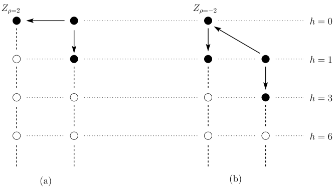
Figure 2: (a) Local martingales of SLE${}_{\kappa=8}(\rho=2)$ form a simple staggered module which coincides with the fusion $\mathcal{Q}_{1,2}\boxtimes\mathcal{Q}_{1,2}$. (b) For SLE${}_{\kappa=8}(\rho=-2)$ we have another staggered module. It now coincides with the fusion $\mathcal{Q}_{1,2}\boxtimes\mathcal{Q}_{2,2}$. We point out that to identify the module in this picture, we had to determine also the value of an invariant $\beta$.

A probabilistic interpretation of the SLE variant used here is also readily available. Indeed, it has been proved that chordal SLE_κ=8 is the the scaling limit of uniform spanning tree Peano curve [LSW04]. But the chordal SLE in $\mathbb{H}$ from $X_{0}$ to $Y_{0}$ (obtained by a Möbius coordinate change from the one towards infinity, Section 2.1.2) is an SLE${}_{\kappa}(\rho=\kappa-6)$. Therefore the variant considered above is nothing but the scaling limit of a uniform spanning tree Peano curve, in $\mathbb{H}$ from $X_{0}$ to $Y_{0}$. The fact that $Y_{0}$ now is the endpoint of the curve also explains the coincidence of weights of the two fields, $h_{x}=h_{y}=h_{1,2}$.

3.6.2 Module of Section 3.4 at $\kappa=8$

A fusion that is almost as simple as the above is $\mathcal{Q}_{\kappa=8;1,2}\boxtimes\mathcal{Q}_{\kappa=8;2,2}$ [GK96]. The weights of the fields to be fused are those of Section 3.4, $h_{x}=h_{1,2}=\frac{-1}{8}$ and $h_{y}=h_{2,2}=\frac{3}{8}$, so we already know that there’s a staggered module of local martingales of SLE${}_{\kappa=8}(\rho=-2)$. Because the Verma modules of weights $h^{+}=0=h_{1,1}$ and $h^{-}=1=h_{2,1}$ are of chain type, we still need to identify the left and right modules, which is easiest done by calculations of graded dimensions

$$\chi_{\mathcal{U}\Lambda}(q)\;=\; \sum_{m\geq 0}\big{(}\mathrm{dim}\;(\mathcal{U}\Lambda)_{[m]}\big{)}q^{m}$$

$$=\; 1+2q+3q^{2}+4q^{3}+7q^{4}+10q^{5}+14q^{6}+\cdots$$

$$\chi_{\mathcal{U}Z}(q)\;=\; \sum_{m\geq 0}\big{(}\mathrm{dim}\;(\mathcal{U}Z)_{[m]}\big{)}q^{m}$$

$$=\; 1+1q+2q^{2}+2q^{3}+4q^{4}+5q^{5}+8q^{6}+\cdots$$

from which we conclude that $\mathcal{U}\Lambda\subset\mathrm{Ker}\;A_{\kappa=8;\rho=-2}$ has the exact sequence

$$0\longrightarrow\mathcal{Q}_{\kappa=8;1,3}\longrightarrow\mathcal{U}\,\Lambda\longrightarrow\mathcal{Q}_{\kappa=8;1,5}\longrightarrow 0\textrm{ .}$$

Both the left and right modules and the invariant $\beta=-1$ (computed in Section 3.4) again agree with results of the fusion products [GK96], and the module is contragredient to itself. Figure 2(b) illustrates the structure.

4 Fusions in percolation with SLE₆ variants

In this section we consider in some more detail the case $\kappa=6$, which is related to critical percolation. When explicit reference to $\kappa$ is omitted in the rest of the section, this is the value meant.

Before turning to our concrete examples in this case, we recall a few particular features of the conformal field theory approaches to percolation. First, it has been accepted for a long time that critical percolation should be described by a conformal field theory of central charge $c=0$. Indeed, one definite success of conformal field theories was Cardy’s exact formula for the crossing probability of a conformal quadrilateral, derived originally from CFT [Car92], immediately supported by numerical evidence [LPPSA92] and later proved rigorously for triangular lattice site percolation [Smi01]. On the other hand, the $c=0$ minimal model would be a trivial theory containing nothing but the identity operator, and as such clearly inadequate. There are no obvious alternative candidates, and for this reason the question of operator content of percolation has received quite a lot of attention recently [MR07, RP07, EF06, RS07]. We will keep these recent studies in mind while exploring the modules of local martingales and their relation to fusion products.

First, to make precise in which sense SLE_κ=6 describes percolation, the discrete site percolation model and result about the scaling limit is recalled in Section 4.1. Having the discrete case in mind allows to interpret the SLE variants in terms of percolation events, which also facilitates comparisons to CFT literature.

We will argue that the module $\mathrm{Ker}\;A$ for ordinary chordal SLE reflects the boundary field of Cardy’s crossing probability argument, in Section 4.2, and for that we exhibit more carefully the degeneracies that even this simplest variant has at rational values. A very simple fusion without logarithms is considered in Section 4.3, again in some detail. There the lesson to take home is that in the space of local martingales, not all null field conditions have yet been taken into account, only the one corresponding to the field at the tip of the curve. Section 4.4 exhibits the simplest way to produce logarithms in percolation CFT. The variant used admits a crossing event interpretation, and the module of local martingales is once again in agreement with CFT fusion prediction. The final example of Section 4.5 is of somewhat speculative nature: we consider a variant of SLE_κ=6 whose local martingales form a module that has been argued to be inconsistent with the percolation CFT, and discuss whether the variant could be made appear in a natural probabilistic setting in percolation.

4.1 The percolation exploration path

A configuration of site percolation on the infinite triangular lattice $T$ is $\sigma\in\{-1,+1\}^{T}$ which is interpreted as a coloring of sites $z\in T$ as black ($\sigma_{z}=-1$) or white ($\sigma_{z}=+1$). It is convenient to think of the sites of the triangular lattice as the faces of the dual, hexagonal lattice $H$, see Figure 3(a). For $p\in[0,1]$ the percolation measure with parameter $p$ is the Bernoulli probability measure with parameter $p$ on the space of configurations $\{-1,+1\}^{T}$, that is we choose the color of each site (hexagon) independently to be white with probability $p$ and black with probability $1-p$. We consider the model at its critical point $p=p_{c}=1/2$.

Figure 3: (a) The sites of triangular lattice are the centers of the faces of hexagonal lattice. (b) The exploration path of percolation separates a “black” cluster from a “white” one. Boundary conditions are “black” on the left and “white” on the right.

The continuum limit corresponds to taking the lattice spacing to zero. Consider therefore the triangular lattice with lattice spacing $\delta$, denoted by $\delta T$. Let $D^{\delta}\subset\delta T$ be a lattice domain, simply connected in the lattice sense and such that the lattice boundary $\partial D^{\delta}$, consisting of sites adjacent to those of the the domain, is a simple lattice path. We imagine splitting the boundary $\partial D^{\delta}$ to two complementary subarcs $\overline{b^{\delta}a^{\delta}}$ and $\overline{a^{\delta}b^{\delta}}$, where $a^{\delta}$ and $b^{\delta}$ are lattice edges ($b^{\delta}$ can be allowed to be at infinity). Consider the percolation configuration restricted to $D^{\delta}$ and extended by black on $\overline{b^{\delta}a^{\delta}}$ and white on $\overline{a^{\delta}b^{\delta}}$. The exploration path of percolation in $D^{\delta}$ from $a^{\delta}$ to $b^{\delta}$ is the maximal dual lattice path $\hat{\gamma}^{\delta}$ starting from $a^{\delta}$ such that each edge of $\hat{\gamma}^{\delta}$ is adjacent to one black and one white site of the above configuration. Figure 3(b) portrays a percolation configuration and the beginning of the corresponding exploration path in $D^{\delta}=\mathbb{H}\cap\delta T$ with $b^{\delta}$ at infinity.

At the critical point, these random paths have a limit for example in the sense of weak convergence of the probability laws on the space of unparametrized paths with the metric

$$d(\gamma^{1},\gamma^{2})\;=\;\underset{\begin{subarray}{c}\textrm{parametrizations}\\ \gamma^{j}=\tilde{\gamma}^{j}[0,1]\end{subarray}}{\inf}\;\sup_{s\in[0,1]}|\tilde{\gamma}^{1}(s)-\tilde{\gamma}^{2}(s)|\textrm{ .}$$

Let $D$ be a Jordan domain (simply connected bounded open set of the plane whose boundary is a simple closed curve) with two distinct boundary points $a,b\in\partial D$. In [Smi01, CN07] it is shown that if one approximates $(D,a,b)$ in a suitable sense by lattice domains $(D^{\delta},a^{\delta},b^{\delta})$, then the laws of the exploration paths $\hat{\gamma}^{\delta}$ of critical percolation in $D^{\delta}$ from $a^{\delta}$ to $b^{\delta}$ converge to the image $f_{D}(\gamma)$ of chordal SLE₆ trace $\gamma$ in $\mathbb{H}$ under any conformal map $f_{D}:\mathbb{H}\rightarrow D$ such that $f_{D}(0)=a$, $f_{D}(\infty)=b$.

The convergence results for exploration path have proved powerful. They have so far been used at least to the mathematical treatments of critical exponents [SW01], one-arm exponent [LSW02], Watts’ crossing formula [Dub06] and surrounding probabilities [Sch01].

4.2 Chordal SLE₆ and Cardy’s boundary field

The result described above allows us to interpret the chordal SLE_κ=6 as the scaling limit of the exploration path as in Figure 3(b).

We have already considered the module of local martingales in the case of chordal SLE_κ, which for irrational $\kappa$ was an irreducible highest weight module with highest weight vector $Z=1$. As mentioned in Section 3.1, in general we have $\mathrm{Ker}\;A_{\kappa}\cong\mathcal{Q}_{1,2}^{*}$. Below we take a closer look at $\kappa=6$ to illustrate the degeneracies that occur at rational values of $\kappa$. There is another important reason to discuss this case: this simple variant which doesn’t yet involve fusions will still teach us something, it will exhibit a representation contragredient to the conformal family of the boundary condition changing field $\psi$ used by Cardy in the derivation of the crossing probability formula.

In our case $\kappa=6$, $h_{1,2}=0=h_{1,1}$ and $\mathcal{Q}_{1,2}$ contains a non-zero singular vector at level $1$, $L_{-1}\,w_{1,2}\neq 0$. At level $2$ there is a null vector, $(L_{-1}^{2}-\frac{2}{3}\,L_{-2})\,w_{1,2}=0$. These properties correspond exactly to what one has to assume of Cardy’s boundary changing field $\psi$ (see [MR07]). It should be a primary field with weight $h=0$ and have a null descendant at level two (leading to a second order differential equation for correlation functions), but it should not be the identity, $L_{-1}\,w_{1,2}\neq 0$ so that $\psi$ is not translation invariant (Cardy’s crossing probability formula is non-constant!).

As $\mathcal{Q}_{1,2}$ is reducible at $\kappa=6$, its contragredient $\mathcal{Q}_{1,2}^{*}$ is not a highest weight representation. The contragredient contains a subrepresentation isomorphic to the irreducible module $\mathcal{L}_{h=0}=\mathcal{U}\,w_{1,2}^{*}\,\subset\,\mathcal{Q}_{1,2}^{*}$ generated by $w^{*}_{1,2}\in(\mathcal{Q}^{*}_{1,2})_{0}$ such that $\big{<}w_{1,2}^{*},w_{1,2}\big{>}=1$ (in this case $\mathcal{L}_{h=0}$ happens to be one dimensional). The full contragredient module is generated by a sub-singular vector $\xi^{*}\in(\mathcal{Q}_{1,2}^{*})_{1}$ that has a nonzero value on the singular vector, $\big{<}\xi^{*},L_{-1}\,w_{1,2}\big{>}=1$. We have $\mathcal{Q}_{1,2}^{*}/\mathcal{L}_{h=0}\cong\mathcal{L}_{h=1}$, or in other words

$$0\longrightarrow\mathcal{L}_{h=0}\longrightarrow\mathcal{Q}_{1,2}^{*}\longrightarrow\mathcal{L}_{h=1}\longrightarrow 0\textrm{ ,}$$

but of course $\mathcal{Q}_{1,2}^{*}$ is not a staggered module: $L_{0}$ is still diagonalizable!

To see $\mathcal{Q}_{1,2}^{*}$ arise as module of SLE local martingales is very easy: the one dimensional module $\mathcal{L}_{h=0}$ is generated by the partition function $Z=1$. To verify that $\mathcal{U}\,Z$ is the irreducible highest weight module we only check

$$L_{2}\;Z=L_{1}\;Z=L_{0}\;Z=L_{-1}\;Z=L_{-2}\;Z\;=\;0\textrm{ .}$$

The function representing $\xi^{*}$ is $\Xi(x,a_{2},a_{3},\ldots)=x$, and the fact that $\Xi\in\mathrm{Ker}\;A$ is just the observation that $X_{t}=\sqrt{6}\;B_{t}$ is a (local) martingale. By the above general arguments we expect that $(\mathcal{U}\,\Xi)/(\mathcal{U}\,Z)\cong\mathcal{L}_{h=1}$. After verifying that $L_{1}\,\Xi=1=Z$, $L_{2}\,\Xi=0$ and $(L_{0}-1)\,\Xi=0$, i.e. that $\Xi$ becomes singular in the quotient, there are several ways to determine the explicit structure of the quotient $(\mathcal{U}\,\Xi)$ by $(\mathcal{U}\,Z)$, which must now be a highest weight module. The result is expected, $(\mathcal{U}\,\Xi)/(\mathcal{U}\,Z)\cong\mathcal{L}_{h=1}$, which is most concretely verified by showing (with the help of a computer) that there are null vectors at the levels $4$ and $6$ (note that $h=1=h_{1,4}=h_{3,2}$)

$$\chi_{1,4}\,\Xi\;=\;0\quad\textrm{ and }\quad\chi_{3,2}\,\Xi\;=\;0\quad\textrm{ , where}$$

$$\chi_{1,4}\;=\; L_{-1}^{4}-\frac{20}{3}\,L_{-2}L_{-1}^{2}+4\,L_{-2}^{2}+4\,L_{-3}L_{-1}-4\,L_{-4}$$

$$\chi_{3,2}\;=\; L_{-1}^{6}-14\,L_{-2}L_{-1}^{4}+\frac{112}{3}\,L_{-2}^{2}L_{-1}^{2}-\frac{512}{27}\,L_{-2}^{3}$$

$$+14\,L_{-3}L_{-1}^{3}-\frac{40}{3}\,L_{-3}L_{-2}L_{-1}-\frac{208}{9}\,L_{-3}^{2}-48\,L_{-4}L_{-1}^{2}$$

$$+\frac{688}{9}\,L_{-4}L_{-2}+\frac{88}{9}\,L_{-5}L_{-1}+\frac{80}{3}\,L_{-6}\textrm{ .}$$

The same conclusion is obtained slightly less explicitly by computing the number of linearly independent functions among $L_{-n_{1}}\cdots L_{-n_{m}}\,\Xi$, with $n_{1}\geq n_{2}\geq\cdots\geq n_{m}>0$ and $\sum_{j}n_{j}=k\geq 0$. Since $\mathcal{U}_{k+1}\,Z=\{0\}$, this gives the graded dimension of $(\mathcal{U}\,\Xi)/(\mathcal{U}\,Z)$

$$\chi_{\mathcal{U}^{-}\,\Xi}(q)\;=\; \sum_{k\geq 0}\big{(}\mathrm{dim}\;(\mathcal{U}\Xi)_{[1+k]}\big{)}\;q^{k}$$

$$\;=\; 1+q+2q^{2}+3q^{3}+4q^{4}+6q^{5}+8q^{6}+\cdots$$

$$\;=\; p(0)+p(1)q+p(2)q^{2}+p(3)q^{3}+(p(4)-p(0))q^{4}$$

$$\qquad+(p(5)-p(1))q^{5}+(p(6)-p(2)-p(0))q^{6}+\cdots\textrm{ .}$$

Yet an alternative argument for which no further calculations are needed relies on the character identity $\chi_{\mathcal{L}_{h=0}}(q)+q\;\chi_{\mathcal{L}_{h=1}}(q)=(1-q^{2})\;\prod_{j=0}^{\infty}(1-q^{j})^{-1}=\chi_{\mathcal{Q}_{1,2}}(q)$. From it we read that if $(\mathcal{U}\,\Xi)/(\mathcal{U}\,Z)$ is irreducible, the graded dimension of $\mathcal{U}\,\Xi$ is that of $\mathrm{Ker}\;A\subset\mathcal{F}^{\mathrm{polyn.}}$ (for which we use the result of [BB03]). If $\chi_{1,4}\,\Xi$ or $\chi_{3,2}\,\Xi$ would not belong to $\mathcal{U}\,Z$ so that the quotient would be reducible, the dimensions would be too large. The structure of the modules is visualized in Figure 4.

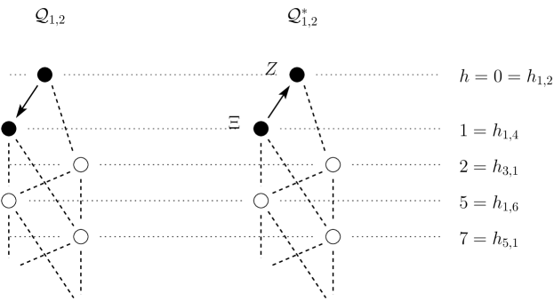
Figure 4: Cardy’s boundary changing field $\psi$ generates a conformal family isomorphic to $\mathcal{Q}_{1,2}$. The chordal SLE_κ=6 local martingales form the contragredient module $\mathcal{Q}_{1,2}^{*}$.

This case of chordal SLE_κ is well understood and not new. But at $\kappa=6$ we’ve seen that it is related to Cardy’s field $\psi$ and can be thought of a concrete verification that the representation $\mathcal{Q}_{1,2}$ appears in percolation. It has been understood already before that Cardy’s field $\psi$ is the boundary condition changing field that changes between fixed black and fixed white boundary conditions, as Figure 3(b) also illustrates.

4.3 SLE${}_{6}(0)$ and fusion of two Cardy’s fields

After arguing the existence of $\mathcal{Q}_{1,2}$, if the CFT is to be closed under fusion, a natural thing to do is to proceed by taking fusion products of this representation as in [MR07]. As a first step one considers $\mathcal{Q}_{1,2}\,\boxtimes\,\mathcal{Q}_{1,2}$, the result of which is $\mathcal{Q}_{1,1}\oplus\mathcal{L}_{h=1/3}$, [MR07, EF06, RS07, RP07].

To study this fusion, we will find an SLE variant where another boundary changing field $\psi$ is present in addition to that at $X_{0}$. In fact, the endpoint (above chosen to be $\infty$) of the curve plays the same role in boundary conditions as the starting point $X_{0}$ and thus in a chordal SLE from $X_{0}=0$ to $Y_{0}\neq 0$ the boundary changing fields on the real axis should provide the two modules we want to fuse. The chordal SLE towards $Y_{0}$ is obtained by a coordinate change as discussed in Section 2.1.2, and is in general an SLE${}_{\kappa}(\rho)$ with $\rho=\kappa-6$. In our case $\kappa=6$ and $\rho=0$ so again the partition function is $Z=1$ and statistics of the driving process are not affected (up to times until which the variant SLE${}_{6}(0)$ is defined). Actually, this curiosity is easily interpreted probabilistically: it is a special case of a property known as the locality of SLE₆. Notice that whether the exploration path takes a left or right turn is determined by the color of hexagon in front of the path, which is chosen independently of other colors. Thus the statistics of the path (up to the time it reaches the changed part of the boundary) is not affected by whether the boundary colors change at $\infty$ or $Y_{0}$.

4.3.1 Local martingales for SLE${}_{6}(0)$

We now consider the process SLE${}_{6}(0)$ and the functions $\varphi(x,y,a_{2},a_{3},\ldots)$ such that $\frac{1}{Z}\,\varphi(X_{t},g_{t}(Y_{0}),a_{2}(t),\ldots)$ are local martingales. If $\varphi$ doesn’t depend on $y$ the question reduces to the one in Section 3.1. In particular the representations found there are contained in $\mathrm{Ker}\;A_{\rho=0}$.

Since the fusion $\mathcal{Q}_{1,2}\,\boxtimes\,\mathcal{Q}_{1,2}$ splits into a direct sum of representations where $L_{0}$ eigenvalues are in $0+\mathbb{N}$ and $\frac{1}{3}+\mathbb{N}$, the contragredient splits accordingly. We start by discussing the former part, $\mathcal{Q}_{1,1}^{*}$. In Section 3.1 we have already found $Z$ and $\Xi$ such that $\mathcal{L}_{h=0}\cong\mathcal{U}\,Z\subset\mathcal{U}\,\Xi\subset\mathrm{Ker}\;A$. In $\mathcal{Q}_{1,1}$ there’s a non-zero singular vector at level $2$ and in $\mathcal{Q}_{1,1}^{*}$ one correspondingly has a sub-singular vector $\theta^{*}\in(\mathcal{Q}_{1,1}^{*})_{2}$. This generates the full representation $\mathcal{U}\,\theta^{*}=\mathcal{Q}_{1,1}^{*}$ and the quotient is $(\mathcal{U}\,\theta^{*})/(\mathcal{U}\,w_{1,1}^{*})\cong\mathcal{L}_{h=2}$. With a little imagination or familiarity with Bessel processes, one finds the corresponding local martingale for SLE, $\frac{1}{5}(X_{t}-Y_{t})^{2}-a_{2}(t)$. Denote $\Theta(x,y,a_{2},a_{3},\ldots)=\frac{1}{5}(x-y)^{2}-a_{2}\in\mathcal{F}$. One explicitly checks that

$$L_{1}\,\Theta=0\qquad L_{2}\;\Theta=1=Z\qquad (L_{0}-2)\,\Theta=0$$

so that $(\mathcal{U}\;\Theta)/(\mathcal{U}\;Z)$ is a highest weight module of weight $h=2=h_{3,1}=h_{1,5}$ and

$$\big{(}L_{-1}^{3}-6\;L_{-2}L_{-1}+6\;L_{-3}\big{)}\;\Theta \;=\;0$$

$$\big{(}L_{-1}^{5}-\frac{40}{3}L_{-2}L_{-1}^{3}+\frac{256}{9}L_{-2}^{2}L_{-1}+\frac{52}{3}L_{-3}L_{-1}^{2}\qquad\qquad$$

$$-\frac{256}{9}L_{-3}L_{-2}-\frac{104}{3}L_{-4}L_{-1}+\frac{208}{9}L_{-5}\big{)}\;\Theta \;=\;0$$

so that there are null vectors at levels $3$ and $5$. We conclude that the module $\mathcal{U}\;\Theta$ is indeed isomorphic to $\mathcal{Q}_{1,1}^{*}$.

The other summand in the $\mathcal{Q}_{1,2}\,\boxtimes\,\mathcal{Q}_{1,2}$ should have $L_{0}$ eigenvalues in $\frac{1}{3}+\mathbb{N}$. It is known in general [BBK05, Kyt07] that the partition function of another double SLE, $\widetilde{Z}=(x-y)^{h_{1,3}-2h_{1,2}}=Z_{\rho=2}$, provides a local martingale $\widetilde{Z}/Z$ for SLE${}_{\kappa}(\kappa-6)$. In our case $\kappa=6$ this means $\widetilde{Z}=(x-y)^{1/3}$. Indeed $A_{\rho=0}\,\widetilde{Z}=0$ and we compute

$$L_{1}\,\widetilde{Z}=0\qquad L_{2}\,\widetilde{Z}=0\qquad (L_{0}-\frac{1}{3})\,\widetilde{Z}=0$$

to see that $\mathcal{U}\,\widetilde{Z}\subset\mathrm{Ker}\;A_{\rho=0}$ is a highest weight module of weight $h=\frac{1}{3}=h_{1,3}$. To check its irreducibility one verifies

$$\big{(}L_{-1}^{3}-\frac{8}{3}L_{-2}L_{-1}+\frac{4}{9}L_{-3}\big{)}\;\widetilde{Z}\;=\; 0\textrm{ .}$$

This is enough since weight $h_{1,3}$ corresponds to a chain type Verma module, whose maximal proper submodule is generated by the grade $3$ singular vector.

4.3.2 Comparison of the fusion and local martingales

We may conclude that $\Theta$ and $\widetilde{Z}$ generate the local martingales that one expects from the fusion $\mathcal{Q}_{1,2}\,\boxtimes\,\mathcal{Q}_{1,2}$

$$\mathrm{Ker}\;A_{\rho=0}\;\supset\;\mathcal{U}\;\Theta\,+\,\mathcal{U}\;\widetilde{Z}\,\cong\,\mathcal{Q}_{1,1}^{*}\,\oplus\,\mathcal{L}_{h=1/3}^{*}\,=\,(\mathcal{Q}_{1,2}\,\boxtimes\,\mathcal{Q}_{1,2})^{*}\textrm{ .}$$

However, it seems fair to ask why the leftmost inclusion is not an equality. For example the local martingale $\Xi$ (and much of the module $\mathcal{U}\,\Xi$ generated by it) does not appear in the contragredient of the fusion product. So in fact $\mathcal{U}\,\Theta$ is naturally included in a larger module $\mathcal{U}\,\Theta+\mathcal{U}\,\Xi\,\subset\,\mathrm{Ker}\;A$. An analogous phenomenon happens with the other part of the direct sum. One may check that $\Upsilon(x,y,a_{2},a_{3},\ldots)=(x-y)^{1/3}(\frac{2}{21}x^{3}+\frac{1}{7}x^{2}y+\frac{3}{7}xy^{2}-a_{3})$ is in $\mathrm{Ker}\;A_{\rho=0}$. Furthermore,

$$L_{1}\,\Upsilon=\big{(}-\frac{45}{7}\,L_{-1}^{2}+\frac{39}{7}\,L_{-2}\big{)}\,\widetilde{Z}\;\in\;\mathcal{U}\,\widetilde{Z}\quad\textrm{ ,}\quad L_{2}\,\Upsilon=0$$

$$(L_{0}-\frac{10}{3})\,\Upsilon=0$$

and $L_{3}\,\Upsilon=\widetilde{Z}$, so we have $\mathcal{L}_{h=1/3}\cong\mathcal{U}\,\widetilde{Z}\subset\mathcal{U}\,\Upsilon$. Since $\Upsilon\notin\mathcal{U}\,\widetilde{Z}$ (one checks that $\mathrm{dim}\;(\mathbb{C}\,\Upsilon+\mathcal{U}_{3}\,\widetilde{Z})=3>2=\mathrm{dim}\;\mathcal{U}_{3}\,\widetilde{Z}$) and $L_{n}\,\Upsilon\in\mathcal{U}\,\widetilde{Z}$ for $n>0$, the quotient $(\mathcal{U}\,\Upsilon)/(\mathcal{U}\,\widetilde{Z})$ is a highest weight module of weight $h=\frac{10}{3}=h_{1,3}+3=h_{1,6}$. Thus also $\mathcal{U}\,\widetilde{Z}$ is naturally contained in a larger module.

To understand why the space of local martingales, $\mathrm{Ker}\;A_{\rho=0}$, is larger than the fusion that we attempted to study, we should take a look back at the constructions [Kyt07] which showed that $\mathrm{Ker}\;A_{\rho=0}$ is a Virasoro module. One notices that there is no need to make any assumptions of the field located at $y$ except that it is a primary field of the correct weight. In particular the null field condition that would be satisfied if the field was $\psi$, corresponding to $\mathcal{Q}_{1,2}$, is not used. We thus expect $\mathrm{Ker}\;A_{\rho=0}$ to rather reflect the fusion $\mathcal{Q}_{1,2}\,\boxtimes\,\mathcal{V}_{h=0}$ than $\mathcal{Q}_{1,2}\,\boxtimes\,\mathcal{Q}_{1,2}$.

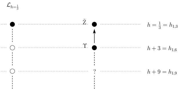
Figure 5: The function $\widetilde{Z}$ generates the irreducible highest weight module $\mathcal{L}_{h=1/3}^{*}\cong\mathcal{L}_{h=1/3}$, the structure of which is portrayed on the left. It is however also contained in a larger module generated by $\Upsilon$ (portrayed on the right). The larger module is not contained in the fusion $\mathcal{Q}_{1,2}\,\boxtimes\,\mathcal{Q}_{1,2}$ (see main text), so we haven’t examined the precise structure of it.

The constructions [Kyt07] do also provide a probabilistic interpretation of guaranteeing the desired null vector condition for the field at $y$. This consists of studying a double SLE (a particular case of multiple SLEs [BBK05]) with the same partition function $Z=(x-y)^{-2h_{1,2}}=1$. The local martingales for this process form a smaller module $\mathrm{Ker}\;A_{\rho=0}\,\cap\,\mathrm{Ker}\;{A^{\downarrow}}_{\rho=0}$, where ${A^{\downarrow}}$ is in fact the generator of the chordal SLE in the reverse direction, from $y$ to $x$

$${A^{\downarrow}}_{\kappa;\rho=\kappa-6} \;=\;\frac{\kappa}{2}\;\frac{\partial^{2}}{\partial y^{2}}+\frac{2}{x-y}\;\frac{\partial}{\partial x}-\frac{2\,h_{1,2}(\kappa)}{(x-y)^{2}}$$

$$+2\sum_{l\geq 2}\Big{(}\sum_{\begin{subarray}{c}0\leq m\leq l-2\\ 0\leq r\leq\lfloor\frac{l-2-m}{2}\rfloor\end{subarray}}y^{m}(-1)^{r}\frac{(m+r)!}{m!\;r!}\sum_{\begin{subarray}{c}k_{1},\ldots k_{r}\geq 2\\ \sum k_{j}=l-m-2\end{subarray}}a_{k_{1}}\cdots a_{k_{r}}\Big{)}\;\frac{\partial}{\partial a_{l}}\textrm{ .}$$

Indeed, ${A^{\downarrow}}\,Z={A^{\downarrow}}\,\Theta=0$ but ${A^{\downarrow}}\,\Xi=2\,(x-y)^{-1}\neq 0$ and ${A^{\downarrow}}\,\Upsilon=\frac{20}{7}\,(x-y)^{4/3}\neq 0$. The unexpected local martingales don’t appear in the double SLE. We conjecture that in general

$$\mathrm{Ker}\;A_{\kappa;\rho=\kappa-6}\,\cap\,\mathrm{Ker}\;{A^{\downarrow}}_{\kappa;\rho=\kappa-6}\;\overset{?}{=}\;(\mathcal{Q}_{\kappa;1,2}\,\boxtimes\,\mathcal{Q}_{\kappa;1,2})^{*}\textrm{ ,}$$

since null field conditions of both fused parts are taken into account in the double SLE local martingales.

4.4 SLE${}_{6}(-2)$ and logarithms through fusion

4.4.1 The simplest fusion to produce logarithms in percolation

The space of local martingales for a correctly chosen SLE variant turned out to be appropriate for the fusion of two Cardy’s fields $\psi$. Of course requiring the fields to form a space that is closed under fusion one should take that result, and further fuse it with the other fields we have already found. The next step in this direction is important as it will show that the CFT of percolation necessarily contains logarithmic operators. As in [MR07] we next address the fusion $\mathcal{Q}_{1,2}\,\boxtimes\,\mathcal{L}_{h=1/3}$, the result of which is a staggered module $\mathcal{S}$ with left and right highest weight modules $\mathcal{Q}_{1,2}$ and $\mathcal{Q}_{1,4}$ respectively, i.e.

$$0\longrightarrow\mathcal{Q}_{1,2}\longrightarrow\mathcal{S}\longrightarrow\mathcal{Q}_{1,4}\longrightarrow 0\textrm{ .}$$

The representation is characterized by giving the invariant $\beta$ defined in Section 2.2. From [MR07] we quote the value $\beta=-\frac{1}{2}$. For later comparison, the graded dimension is

$$\chi_{\mathcal{S}}(q)\;=\; \sum_{k\geq 0}(\mathrm{dim}\;\mathcal{S}_{[k]})\;q^{k}\;=\;\sum_{k\geq 0}\big{(}\mathrm{dim}\;(\mathcal{Q}_{1,2})_{k}+\mathrm{dim}\;(\mathcal{Q}_{1,4})_{k-1}\big{)}\;q^{k}$$

$$=\; 1+2q+2q^{2}+4q^{3}+6q^{4}+8q^{5}+12q^{6}+17q^{7}+23q^{8}+\cdots\textrm{ .}$$

4.4.2 An SLE variant that describes a crossing event

We’d again like to find a probabilistic setup for studying the fusion $\mathcal{Q}_{1,2}\,\boxtimes\,\mathcal{L}_{h=1/3}$. The starting point of the SLE curve (or exploration path) provides the field $\psi$ corresponding to $\mathcal{Q}_{1,2}$ and at another point we should have a primary field of conformal weight $h=1/3$. In SLE${}_{\kappa}(\rho)$ the boundary change at $Y_{0}$ is a primary with weight $h(\rho)=\frac{\rho(\rho+4-\kappa)}{4\kappa}$, so we should choose $\rho=-2$ or $\rho=4$. Luckily, the case $\rho=-2$ has already been studied in Section 3.4 and even the probabilistic interpretation has been discussed in Section 2.1.2: we know that it describes an ordinary chordal SLE_κ from $X_{0}$ to $Y_{0}$ in $\mathbb{H}$, conditioned to reach the endpoint $Y_{0}$ without touching the interval $(Y_{0},\infty)$.

In view of the discrete definition of the percolation exploration process, the event on which we condition can be made more transparent. The complementary event that the exploration path would reach $(Y_{0},\infty)$ before $Y_{0}$ means the existence of a connected white cluster that joins $(X_{0},Y_{0})$ to $(Y_{0},\infty)$ — indeed the hexagons that are immediately on the right of the exploration path belong to such a cluster (compare with Figure 3(b)). The event on which we condition should prevent the above kind of white cluster, by having a black cluster from exactly $Y_{0}$ (a single hexagon, say) to the interval $(-\infty,X_{0})$.

In fact the discrete lattice introduced a microscopic length scale $\delta$, the size of the single hexagon. This suggests that a naive equivalent in the continuum description is to require crossing from $(-\infty,X_{0})$ to $(Y_{0}^{-},Y_{0}^{+})$, where $Y_{0}^{\pm}\approx Y_{0}$ with $Y_{0}^{+}-Y_{0}^{-}=\delta$. This is a crossing event à la Cardy, and in the limit $\delta\rightarrow 0$ one brings two of the “corners” of the conformal quadrilateral together. Conditioning SLE₆ on Cardy’s crossing event is in fact easily done: the SLE variant will have partition function given by Cardy’s formula, $Z(x,y_{-},y_{+})\,=\,\mathsf{P}[\textrm{crossing}]\,=\,F(\frac{y_{-}-x}{y_{+}-x})$, where

$$F(r)\;=\;\frac{\Gamma(\frac{2}{3})}{\Gamma(\frac{1}{3})^{2}}\;\int_{r}^{1}s^{-2/3}(1-s)^{-2/3}\;\mathrm{d}s\textrm{ .}$$

Girsanov’s formula gives the drift of the driving process under the conditioned measure, $\kappa\;\frac{\partial}{\partial x}\log Z(x,y_{-},y_{+})$ and in the limit $y_{-},y_{+}\rightarrow y$ it tends to $\frac{-2}{x-y}$, i.e. the conditioned process indeed tends to SLE${}_{6}(-2)$.

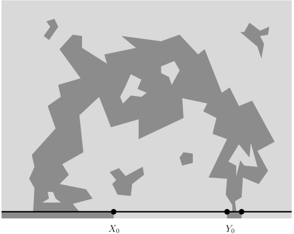
Figure 6: The variant SLE${}_{6}(-2)$ can be obtained by conditioning on a crossing event from a tiny interval around $Y_{0}$ to $(-\infty,X_{0})$. The picture clearly suggests that we’re bringing two Cardy’s color changing boundary fields $\psi$ together at this point. The conditioning picks the component $h=1/3$ instead of $h=0$ from the fusion of two $\psi$ fields at $Y_{0}$.

4.4.3 Local martingales for SLE${}_{6}(-2)$

For the module of local martingales $\mathrm{Ker}\;A_{\kappa=6;\rho=-2}$ we can already quote many results from Section 3.4. The partition function $Z_{\rho=-2}=(x-y)^{-1/3}$ generates a highest weight module with $h=0$ and it has a nonzero singular vector at grade $1$. The singular is in fact the partition function for the choice $\rho=4$, $L_{-1}Z_{\rho=-2}=-\frac{1}{3}Z_{\rho=4}$, where $Z_{\rho=4}=(x-y)^{2/3}$. The operator $A_{\rho=-2}\,=\,A_{\rho=4}$ is the same for the two processes, while the local martingales of the two differ by a factor $Z_{\rho=4}/Z_{\rho=-2}=(x-y)$ (recall that what we abusively called the space of local martingales consists of functions that should still be divided by the partition function to obtain actual local martingales). It is now immediate that $A_{\rho=-2}\;Z_{\rho=-2}\,=\,A_{\rho=-2}\;Z_{\rho=4}\,=\,0$. Observe also that the formulas for $L_{n}$ are the same for these two SLE${}_{6}(\rho)$ processes.

We complete the analysis of Section 3.4 in this degenerate case at $\kappa=6$. To determine completely the structure of the highest weight representation $\mathcal{U}\,Z_{\rho=-2}$ we compute

$$\big{(}L_{-1}^{2}-\frac{2}{3}L_{-2}\big{)}\,Z_{\rho=-2}=0$$

which confirms that $\mathcal{U}\,Z_{\rho=-2}\,\cong\,\mathcal{Q}_{1,2}$. Without further computations one concludes the irreducibility of $\mathcal{U}\,Z_{\rho=4}\,\cong\,\mathcal{L}_{h=1}$, although one can also check directly the existence of null vectors at levels $4$ and $6$.

The logarithmic partner to $L_{-1}Z_{\rho=-2}$ is $\Lambda$, and we have computed

$$(L_{0}-1)\;\Lambda\,=\,L_{-1}\;Z_{\rho=-2}\quad\textrm{ and }\quad L_{1}\;\Lambda\,=\,-\frac{1}{2}Z_{\rho=-2}\textrm{ .}$$

The latter already says that the invariant takes the same value as in the corresponding fusion, $\beta=-1/2$, although we still haven’t got enough information to decide the structure of the right module. By a computer assisted computation one obtains the numbers of linearly independent local martingales by grade,

$$\chi_{\mathcal{U}\,\Lambda}(q)\;=\; \sum_{k\geq 0}\Big{(}\mathrm{dim}\;\big{(}\mathcal{U}^{-}_{k-1}\,\Lambda+\mathcal{U}^{-}_{k}\,Z_{\rho=-2}\big{)}\Big{)}\;q^{k}$$

$$=\; 1+2q+2q^{2}+4q^{3}+6q^{4}+8q^{5}+12q^{6}+17q^{7}+\cdots\textrm{ ,}$$

in agreement with the character of the module $\mathcal{S}$. Noting the graded dimensions of the left highest weight module $\mathcal{U}\,Z_{\rho=-2}$ (which can be computed directly, but also follows from the earlier verification of $\mathcal{U}Z_{\rho=-2}=\mathcal{Q}_{1,2}$)

$$\chi_{\mathcal{U}\,Z_{\rho=-2}}(q)\;=\; \sum_{k\geq 0}\mathrm{dim}\;\big{(}\mathcal{U}^{-}_{k}\,Z_{\rho=-2}\big{)}\;q^{k}$$

$$=\; 1+1q+1q^{2}+2q^{3}+3q^{4}+4q^{5}+6q^{6}+8q^{7}+\cdots$$

we deduce the graded dimension of the quotient $(\mathcal{U}\,\Lambda)/(\mathcal{U}\,Z_{\rho=-2})$

$$\sum_{k\geq 0}\Big{(}\mathrm{dim}\;\big{(}\mathcal{U}^{-}_{k}\,\Lambda+\mathcal{U}^{-}_{k+1}\,Z_{\rho=-2}\big{)}\;-\;\mathrm{dim}\;\mathcal{U}^{-}_{k+1}\,Z_{\rho=-2}\Big{)}\;q^{k}$$

$$=\; 1+q+2q^{2}+3q^{3}+4q^{4}+6q^{5}+9q^{6}+\cdots$$

$$=\; p(0)+p(1)q+p(2)q^{2}+p(3)q^{3}+(p(4)-p(0))q^{4}$$

$$\qquad+(p(5)-p(1))q^{5}+(p(6)-p(2))q^{6}+\cdots\textrm{ .}$$

This confirms that the quotient is isomorphic to $\mathcal{Q}_{1,4}$: at grade $4$ there is a null vector whereas at grade $6$ there is a non-zero singular vector (corresponding to a sub-singular vector at grade $7$ of the staggered module $\mathcal{U}\,\Lambda$).

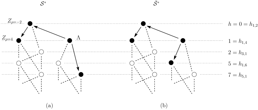
Figure 7: (a) The local martingales for SLE${}_{6}(-2)$ contain a staggered module $\mathcal{S}^{*}$ contragredient to the fusion $\mathcal{Q}_{1,2}\,\boxtimes\,\mathcal{L}_{h=1/3}\;=\;\mathcal{S}$. (b) A very similar staggered module of local martingales is found for the SLE variants of Section 4.5. The existence of such a module in the conformal field theory of percolation has been argued to be impossible.

Above, we have effectively shown that $\mathcal{U}\Lambda\subset\mathrm{Ker}\;A_{\kappa=6;\rho=-2}$ is isomorphic to the result of the fusion $\mathcal{Q}_{1,2}\,\boxtimes\,\mathcal{L}_{h=1/3}$. This is not exactly what we claimed, as we have not yet taken contragredients. But just like in Section 3.5, elementary means allow to check that the module is contragredient to itself. A small difference is that we must now show that $\mathcal{U}\xi^{*}$ has a null vector at grade $2$, which however follows rather directly from graded dimensions. Indeed, we know that $\mathcal{U}\xi^{*}$ and $\mathcal{U}\eta^{*}/\mathcal{U}\xi^{*}$ are highest weight modules of highest weights $0$ and $1$ respectively, so the inequality $2=\mathrm{dim}\;(\mathcal{U}\Lambda)_{[2]}\geq\mathrm{dim}\;(\mathcal{U}\eta^{*}/\mathcal{U}\xi^{*})_{[2]}+\mathrm{dim}\;(\mathcal{U}\xi^{*})_{[2]}=1+\mathrm{dim}\;(\mathcal{U}\xi^{*})_{[2]}$ leaves no other possibility but to have a null vector $(L_{-1}^{2}-\frac{2}{3}L_{-2})\xi^{*}=0$ (the grade one singular $L_{-1}\xi^{*}$ is non-zero by earlier analysis). Similarly, graded dimensions also imply that $\mathcal{U}\eta^{*}/\mathcal{U}\xi^{*}$ must have a null vector at grade $4$. The last remaining check of non-zero singular vector at grade $6$ can be done mechanically We then conclude that the contragredient to the appropriate fusion product has been realized as local martingales again,

$$(\mathcal{Q}_{1,2}\,\boxtimes\,\mathcal{L}_{h=1/3})^{*}\cong\mathcal{U}\,\Lambda\,\subset\,\mathrm{Ker}\;A_{\rho=-2}\textrm{ .}$$

4.5 On the question of existence of $\mathcal{Q}_{2,1}$

In [MR07] it is argued that a consistent chiral CFT with $c=0$ can’t contain both $\mathcal{Q}_{1,2}$ (the Cardy’s field) and $\mathcal{Q}_{2,1}$. The question of whether $\mathcal{Q}_{2,1}$ is present in percolation CFT has nevertheless been subject to some discussion, as for example building modular invariant partition function seems to require the character of $\mathcal{Q}_{2,1}$ [Flo]. The percolation literature also contains some references to fields of dimension $h=h_{2,1}=\frac{5}{8}$, e.g. [CZ92]. In the SLE context a natural way for $\mathcal{Q}_{2,1}$ to appear would be through Duplantier duality $\kappa\leftrightarrow\frac{16}{\kappa}=\kappa^{*}$, see [Dup00, Zha08a, Zha08b, Dub07b], although this doesn’t directly give an interpretation of it as a boundary condition changing field for percolation, either. Below we will outline a possible way to gain some understanding of this question from the point of view of the local martingales of SLE variants involving both $\kappa=6$ and the dual value $\kappa^{*}=\frac{8}{3}$.

4.5.1 The conflicting module

The inconsistency of adding $\mathcal{Q}_{2,1}$ to the theory ultimately boils down to the observation that it would lead, through fusions, to the existence of staggered modules with logarithmic couplings different from what is produced by the fusions generated by $\mathcal{Q}_{1,2}$ alone. This is argued to contradict requirements of chiral conformal field theory [MR08]. From SLE point of view perhaps the simplest such conflicting module arises in the fusion $\mathcal{Q}_{1,2}\;\boxtimes\;\mathcal{Q}_{2,1}\;\boxtimes\;\mathcal{Q}_{2,1}$. From the computations in [MR08] and associativity of fusion product one finds that this fusion contains a staggered module $\widetilde{\mathcal{S}}$ characterized by the exact sequence $0\rightarrow\mathcal{Q}_{1,2}\rightarrow\widetilde{\mathcal{S}}\rightarrow\mathcal{Q}_{3,2}\rightarrow 0$ and logarithic coupling $\widetilde{\beta}=1/3$, i.e. $L_{1}\,\eta=\frac{1}{3}\,\xi$. The structure of this staggered module is very similar to that of $\mathcal{S}$ in Section 4.4, see Figure 7, but the logarithmic couplings are different $\beta\neq\widetilde{\beta}$.

There are several possibile SLE₆ variants that reflect the fusion $\mathcal{Q}_{1,2}\,\boxtimes\,\mathcal{Q}_{2,1}\,\boxtimes\,\mathcal{Q}_{2,1}$, for example SLE${}_{\kappa=6}(\rho_{1}=-3,\rho_{2}=-3)$ with partition function

$$Z_{\underline{\rho}=(-3,-3)}\;=\;\frac{(y_{1}-y_{2})^{3/4}}{(x-y_{1})^{1/2}\;(x-y_{2})^{1/2}}\textrm{ .}$$

This is a highest weight vector of $L_{0}$ eigenvalue $1=h_{3,2}=h_{1,4}$.

In $\mathrm{Ker}\;A_{\kappa=6;\underline{\rho}=(-3,-3)}$ we find also another highest weight vector

$$F\;=\;\frac{y_{1}+y_{2}-2x}{(x-y_{1})^{1/2}\;(x-y_{2})^{1/2}\;(y_{1}-y_{2})^{5/4}}\textrm{ ,}$$

which could serve as a partition function of an SLE variant as well. The highest weight is $0=h_{1,1}=h_{1,2}$ and the level $1$ singular vector is non-vanishing and in fact proportional to the above partition function $L_{-1}\,F=\frac{1}{2}\,Z_{\underline{\rho}=(-3,-3)}$. We have $(L_{-1}^{2}-\frac{2}{3}L_{-2})\,F=0$ so that $\mathcal{U}\,F\cong\mathcal{Q}_{1,2}$. Since we’re looking for $\widetilde{\mathcal{S}}^{*}$, the task now is to find the logarithmic partner $\Lambda$ of $Z_{\underline{\rho}=(-3,-3)}$.

We note that $F$ and $Z_{\underline{\rho}=(-3,-3)}$ are annihilated by $A_{\kappa=6;\underline{\rho}=(-3,-3)}$, as they should. But moreover they satisfy constraints of the null vectors in $\mathcal{Q}_{2,1}$: they are annihilated also by the generators $A^{(y_{j})}_{\kappa=8/3;\underline{\rho}=(2,-4/3)}$ ($j=1,2$) of SLE_8/3 variants started from $y_{1}$ and $y_{2}$ with the same partition function. Also the logarithmic partner becomes determined (up to the usual freedom in the choice of $\eta$) if we require that it is in $\mathrm{Ker}\;A_{\kappa=6;\underline{\rho}=(-3,-3)}\;\cap\;\mathrm{Ker}\;A^{(y_{j})}_{\kappa=8/3;\underline{\rho}=(2,-4/3)}$ (either one of $j$ equals $1$ or $2$ is enough, the other then follows). We can choose

$$\Lambda\;=\;\frac{2\,x\,(y_{1}+y_{2}-2x)\;+\;3(y_{1}-y_{2})^{2}\,\log(y_{1}-y_{2})}{6\,(x-y_{1})^{1/2}\;(x-y_{2})^{1/2}\;(y_{1}-y_{2})^{5/4}}\textrm{ .}$$

This choice satisfies the normalization $(L_{0}-1)\,\Lambda=L_{-1}\,F$ and the logarithmic coupling is $\widetilde{\beta}=\frac{1}{3}$ as follows from $L_{1}\,\Lambda=\frac{1}{3}F$.

It turned out to be computationally slightly too demanding to verify that the quotient $(\mathcal{U}\,\Lambda)/(\mathcal{U}\,F)$ possesses a non zero singular vector at level $4$ and a null vector at level $6$. But accepting that, one would conclude that $\mathcal{U}\,\Lambda$ is isomorphic to the contragredient of the staggered module $\widetilde{\mathcal{S}}$ which appears in the fusion $\mathcal{Q}_{1,2}\,\boxtimes\,\mathcal{Q}_{2,1}\,\boxtimes\,\mathcal{Q}_{2,1}$.

4.5.2 Interpreting the variants in percolation

Some experts of the conformal field theory approach to percolation have found the above discussion of the conflicting module through multiple SLEs confusing. What we have shown so far is that there are multiple SLE variants involving SLE type curves with both $\kappa=6$ and $\kappa=\frac{8}{3}$ whose local martingales contain the staggered module $\widetilde{\mathcal{S}}$ (one can choose as partition function any linear combination of $F$ and $Z_{\kappa=6;\underline{\rho}=(-3,-3)}$) — and nothing yet about its relation to percolation. Now in order to be specific, we will present a definite conjecture that would relate the above multiple SLE variant with partition function $F$ to a reasonable question about triangular lattice site percolation. Of course in doing so we risk being incorrect at several places — more careful research may then either clarify and correct the claims made, or show them altogether wrong.

We start with comments on the roles on boundary conditions of $\mathcal{Q}_{1,2}$ and $\mathcal{Q}_{2,1}$. The interpretation of $\mathcal{Q}_{1,2}$ (Cardy’s field) has become quite clear by now: it corresponds to the starting of an exploration path from boundary point at which the boundary colors change. If we were to choose the variant with partition function $F$, the field at infinity would also have this weight $h=h_{1,2}=0$. To interpret $\mathcal{Q}_{2,1}$ we turn to a duality for conformally invariant random fractals that was observed by Duplantier [Dup00]. Precise proofs in the SLE context have been given in [Zha08a, Zha08b, Dub07b], and they relate SLE_κ to SLE${}_{\kappa^{*}}$, where $\kappa^{*}=\frac{16}{\kappa}$. Roughly speaking the relation is that for $\kappa>4$, the boundary of the region surrounded by SLE_κ trace looks locally like SLE${}_{\kappa^{*}}$. Therefore, since $h_{2,1}(\kappa)=h_{1,2}(\kappa^{*})$ is the conformal weight of the operator at the starting point of SLE${}_{\kappa^{*}}$, the boundary changing fields $\mathcal{Q}_{2,1}$ may correspond to points at which an external perimeter (this should be the correct percolation analogue of the boundary of the region surrounded by the exploration path [ADA99]) of a percolation cluster reaches the boundary.

Guided by the above discussion let us imagine the following situation in triangular lattice site percolation in $D^{\delta}=\mathbb{H}\cap\delta T$. The boundary hexagons are chosen black on $(-\infty,x^{\delta})\cup(y_{1}^{\delta},y_{2}^{\delta})$, and white on $(x^{\delta},y_{1}^{\delta})\cup(y_{2}^{\delta},\infty)$, where $x^{\delta}<y_{1}^{\delta}<y_{2}^{\delta}$. We can define the external perimeter of the white cluster (for example) as the simple lattice path on white hexagons that starts from $(x^{\delta},y_{1}^{\delta})$ and ends on $(y_{2}^{\delta},\infty)$ and surrounds the minimal number of hexagons (so it follows as closely as possible the finite black cluster, but due to the requirements that it is simple and uses only white sites, it can’t enter the fjords). Now condition on the event that this external perimeter starts precisely at the hexagon on the left of $y_{1}^{\delta}$ and ends precisely at the hexagon on the right of $y_{2}^{\delta}$.

In the above situation one can start tracing three random curves from the boundary: the exploration path from $x^{\delta}$, or the external perimeter from either of its two ends $y_{1}^{\delta}$ or $y_{2}^{\delta}$. Now there are two important questions: does the joint law of these curves have a scaling limit as $\delta\searrow 0$ and $(x^{\delta},y_{1}^{\delta},y_{2}^{\delta})\rightarrow(x,y_{1},y_{2})$, and if it does, is it conformally invariant. Supposing the answer to both is affirmative, one would expect the exploration path still to look locally like an SLE_κ=6, while a segment from either end of the external perimeter should look like SLE_κ=8/3. Furthermore, the curves are to be built on the same probability space, so multiple SLEs [BBK05, Gra07] (or a commuting SLE in the terminology of [Dub07a]) seem like plausible candidates for the joint law. There are two linearly independent possibilities for partition functions of such variants of multiple SLEs: $Z_{\kappa=6;\underline{\rho}=(-3,-3)}$ and $F$. The asymptotics of these as $|y_{2}-y_{1}|\rightarrow 0$ are different. By methods similar to [BBK05] one can then argue that only $F$ corresponds to a growth process in which the $\kappa^{*}=\frac{8}{3}$ curves from $y_{1}$ and $y_{2}$ will meet, as they should if they are the two ends of the external perimeter of a black cluster that doesn’t reach to infinity.

To summarize, the conjecture is that if we condition percolation on the event that the external perimeter of a black cluster attached to $(y_{1},y_{2})$ extends precisely from $y_{1}$ to $y_{2}$, then the scaling limit of the three curves is the multiple SLE with partition function $F$. Although there are situations where discrete interfaces have been proved to have scaling limit described by SLE curves, the present conjecture (even if correct) is probably too complicated for rigorous methods. It would nevertheless be very interesting to gain any probabilistic understanding of the case, and to better understand the relation to the inconsistency argument that would ban $\widetilde{\mathcal{S}}$ from the conformal field theory of percolation.

4.6 On the operator content of percolation

Above we considered the simplest but arguably the most fundamental fusions in the conformal field theory of percolation along the lines of the recent study [MR07]. For each of these cases, an SLE variant with a clear interpretation in terms of percolation was found, and local martingales of that variant coincided with the contragredient of the fusion product. This can be thought of as a confirmation of the results, and as a direct link from the discrete percolation model to the operator content question. However, we also presented a conjecture that some situations in percolation are described by the multiple SLEs whose module of local martingales has a structure conflicting consistent chiral CFT.

We remark that in the quest for better understanding the conformal field theory of percolation there are still issues to be solved, notably modular invariance poses a challenge in logarithmic conformal field theories [FGST06, FG06, Flo]. Whether the present approach will be useful to resolve these or other questions remains to be seen, but the present note nevertheless seems to provide a new perspective to the topic.

5 Discussion and conclusions

In this note we studied the local martingales of the SLE_κ growth processes. The space of local martingales forms a Virasoro module, whose structure we examined in several cases. We were particularly interested in a phenomenon encountered in logarithmic conformal field theory, namely non-diagonalizability of $L_{0}$. It was observed that this takes place in natural SLE variants, and at all values of $\kappa>0$ and therefore at all central charge $c\leq 1$. As a byproduct, we obtained values of logarithmic couplings (invariants of the representations) by easy calculations. These values generalized conjectured infinite series of logarithmic couplings for logarithmic M$(2,p)$ minimal models. The calculations in our case were rather harmless, so there is a prospect that similar methods might provide easy access to the more general conjectures made in [MR08].

In all the considered cases, a close relation between the local martingales and the fusion product of boundary condition changing fields was found (the fusion products have been computed in the CFT literature [Gab94, GK96, EF06, RS07, RP07, MR07, MR08]). The contragredient of the fusion product module could be realized as local martingales. We conjecture that this will hold in general, i.e. for any SLE variant. In fact the local martingale condition is closely related to a null descendant of one of the boundary fields — for fusions of several fields with null descendant, appropriate intersections of modules should be taken, as we illustrated with an example of double SLE. It would be interesting to see if the relationship may lend to alternative definitions of fusion, or at least to efficient computational methods to study fusions.

We considered in some detail the case $\kappa=6$, for which SLE describes the scaling limit of critical percolation exploration path. We compared the results to the recent computations of fusion algebra of percolation [MR07, RP07, EF06, RS07], and found agreement in the above mentioned sense. In the cases of the most fundamental fusions, we exhibited probabilistic interpretations of the SLE variants used. For example, logarithms first arise in a SLE variant that is obtained by conditioning on a crossing event. We also exhibited SLE variants whose local martingales form a staggered module whose existence in the CFT of percolation has previously been argued impossible, and discussed whether this variant could nevertheless describe some situations in percolation.

The main philosophical message of the note is the relation of SLEs to logarithmic conformal field theories. Indications of this sort of relation have been observed in different ways in [SAPR09, CS08], and in fact it has been suggested that the CFT description of non-local questions (such as those of the SLE curve) must typically be logarithmic. It is reassuring that the different approaches point to a similar conclusion, and having these different perspectives should be useful when the relation of SLE and LCFT will be better studied in the future.

Acknowledgements: First of all I wish to thank Michel Bauer and David Ridout for numerous interesting discussions at all stages of the research. I am grateful to Annekathrin Müller-Lohmann for explanations on logarithmic conformal field theory and to Hans Plesner Jakobsen for pointing out a misconception of mine about representation theory. I thank Aapo Kyrölä for his patience in giving programming related advice. Michel Bauer, David Ridout and Michael Flohr made valuable comments about the first version of the manuscript.

This work was partly done at the Laboratoire de Physique Théorique et Modèles Statistiques (Université Paris Sud 11) and partly at Section de Mathématiques (Université de Genève) and supported by ENRAGE European Network MRTN-CT-2004-5616, Swiss National Science Foundation and European Research Council.

References

- [ADA99] M. Aizenman, B. Duplantier and A. Aharony, Path-Crossing Exponents and the External Perimeter in 2D Percolation, Phys. Rev. Lett. 83(7), 1359 – 1362 (1999).
- [Ast97] A. Astashkevich, On the structure of Verma modules over Virasoro and Neveu-Schwarz algebras, Comm. Math. Phys. 186(3), 531–562 (1997), [arXiv:hep-th/9511032].
- [BB03] M. Bauer and D. Bernard, SLE martingales and the Virasoro algebra, Phys. Lett. B 557(3-4), 309–316 (2003), [arXiv:hep-th/0301064].
- [BB04] M. Bauer and D. Bernard, Conformal transformations and the SLE partition function martingale, Ann. Henri Poincaré 5(2), 289–326 (2004), [arXiv:math-ph/0305061].
- [BB06] M. Bauer and D. Bernard, 2D growth processes: SLE and Loewner chains, Phys. Rep. 432(3-4), 115–222 (2006), [arXiv:math-ph/0602049].
- [BBK05] M. Bauer, D. Bernard and K. Kytölä, Multiple Schramm-Loewner evolutions and statistical mechanics martingales, J. Stat. Phys. 120(5-6), 1125–1163 (2005), [arXiv:math-ph/0503024].
- [BPZ84] A. A. Belavin, A. M. Polyakov and A. B. Zamolodchikov, Infinite conformal symmetry in two-dimensional quantum field theory, Nucl. Phys. B 241(2), 333–380 (1984).
- [Car92] J. L. Cardy, Critical percolation in finite geometries, J. Phys. A 25, L201–206 (1992), [arXiv:hep-th/9111026].
- [Car99] J. L. Cardy, Logarithmic correlations in quenched random magnets and polymers, [arXiv:cond-mat/9911024], 1999.
- [CN07] F. Camia and C. M. Newman, Critical Percolation Exploration Path and SLE6: a Proof of Convergence, Probab. Theory Related Fields 139(3-4), 473–519 (2007), [arXiv:math/0604487].
- [CS08] J. Cardy and J. J. H. Simmons, Twist operator correlation functions in loop models, [arXiv:0811.4767], 2008.
- [CZ92] L. Chim and A. Zamolodchikov, Integrable Field Theory of the q-state Potts Model with 0<q<4, Int. J. Mod. Phys. A 7(21), 5317–5335 (1992).
- [DFMS97] P. Di Francesco, P. Mathieu and D. Sénéchal, Conformal Field Theory, Springer Verlag, New York, 1997.
- [Dub05] J. Dubédat, martingales and duality, Ann. Probab. 33(1), 223–243 (2005), [arXiv:math.PR/0303128].
- [Dub06] J. Dubédat, Excursion decompositions for SLE and Watts’ crossing formula, Probab. Theory Related Fields 134(3), 453–488 (2006).
- [Dub07a] J. Dubédat, Commutation relations for SLE, Comm. Pure and Applied Math. 60(12), 1792 – 1847 (2007), [arXiv:math.PR/0411299].
- [Dub07b] J. Dubédat, Duality of Schramm-Loewner Evolutions, [arXiv:0711.1884], 2007.
- [Dup00] B. Duplantier, Conformally Invariant Fractals and Potential Theory, Phys. Rev. Lett. 84(7), 1363–1367 (Feb 2000).
- [EF06] H. Eberle and M. Flohr, Virasoro representations and fusion for general augmented minimal models, J. Phys. A: Math. Gen. 39, 15245–15286 (2006), [arXiv:hep-th/0604097].
- [FF83] B. L. Feĭgin and D. B. Fuks, Verma modules over a Virasoro algebra, Funktsional. Anal. i Prilozhen. 17(3), 91–92 (1983).
- [FF84] B. L. Feĭgin and D. B. Fuchs, Verma modules over the Virasoro algebra, in Topology (Leningrad, 1982), volume 1060 of Lecture Notes in Math., pages 230–245, Springer, Berlin, 1984.
- [FF90] B. L. Feĭgin and D. B. Fuchs, Representations of the Virasoro algebra, in Representation of Lie groups and related topics, volume 7 of Adv. Stud. Contemp. Math., pages 465–554, Gordon and Breach, New York, 1990.
- [FG06] M. Flohr and M. Gaberdiel, Logarithmic torus amplitudes, J. Phys. A: Math. Gen. 39, 1955–1968 (2006), [arXiv:hep-th/0509075].
- [FGST06] B. Feigin, A. Gainutdinov, A. Semikhatov and I. Tipunin, Logarithmic extensions of minimal models: characters and modular transformations, Nucl. Phys. B 757(4), 303–343 (2006).
- [Flo] M. Flohr, private communication.
- [Gab94] M. Gaberdiel, Fusion in conformal field theory as the tensor product of the symmetry algebra, Int. J. Mod. Phys. A9, 4619–4636 (1994), [arXiv:hep-th/9307183].
- [GK96] M. Gaberdiel and H. Kausch, Indecomposable fusion products, Nucl. Phys. B 477, 293–318 (1996), [arXiv:hep-th/9604026].
- [Gra07] K. Graham, On Multiple Schramm-Loewner Evolutions, Journal of Statistical Mechanics: Theory and Experiment P03008 (2007), [arXiv:math-ph/0511060].
- [Gur93] V. Gurarie, Logarithmic operators in conformal field theory, Nucl. Phys. B 410, 535–549 (1993), [arXiv:hep-th/9303160].
- [Kau00] H. Kausch, Symplectic fermions, Nucl. Phys. B 583, 513–541 (2000), [arXiv:hep-th/0003029].
- [KK06] K. Kytölä and A. Kemppainen, SLE local martingales, reversibility and duality, J. Phys. A: Math. Gen. 39(46), L657–666 (2006), [arXiv:math-ph/0605058].
- [KN04] W. Kager and B. Nienhuis, A guide to stochastic Löwner evolution and its applications, J. Stat. Phys. 115(5-6), 1149–1229 (2004), [arXiv:math-ph/0312056].
- [KR09] K. Kytölä and D. Ridout, On staggered indecomposable Virasoro modules, [arXiv:0905.0108], 2009.
- [Kyt06] K. Kytölä, Conformal Field Theory Methods for Variants of Schramm-Loewner Evolutions, PhD thesis, University of Helsinki, Department of Mathematics and Statistics, 2006.
- [Kyt07] K. Kytölä, Virasoro module structure of local martingales of SLE variants, Rev. Math. Phys. 19(5), 455–509 (2007), [arXiv:math-ph/0604047].
- [Loe23] K. Löwner, Untersuchungen über schlichte konforme Abbildungen des Einheitskreises I, Math. Ann. 89, 103–121 (1923).
- [Law05] G. F. Lawler, Conformally invariant processes in the plane, volume 114 of Mathematical Surveys and Monographs, American Mathematical Society, Providence, RI, 2005.
- [LPPSA92] R. P. Langlands, C. Pichet, P. Pouliot and Y. Saint-Aubin, On the Universality of Crossing Probabilities in Two-Dimensional Percolation, J. Stat. Phys. 67(3-4) (1992).
- [LSW02] G. F. Lawler, O. Schramm and W. Werner, One-arm exponent for critical 2D percolation, Electron. J. Probab. 7, no. 2, 13 pp. (electronic) (2002), [arXiv:math.PR/0108211].
- [LSW04] G. F. Lawler, O. Schramm and W. Werner, Conformal invariance of planar loop-erased random walks and uniform spanning trees, Ann. Probab. 32(1B), 939–995 (2004), [arXiv:math.PR/0112234].
- [MARR04] S. Moghimi-Araghi, M. A. Rajabpour and S. Rouhani, Logarithmic Conformal Null Vectors and SLE, Phys. Lett. B 600, 297–301 (2004), [arXiv:hep-th/0408020].
- [MR07] P. Mathieu and D. Ridout, From percolation to logarithmic conformal field theory, Phys. Lett. B 657, 120–129 (2007), [arXiv:0708.0802].
- [MR08] P. Mathieu and D. Ridout, Logarithmic M(2,p) Minimal Models, their Logarithmic Couplings, and Duality, Nucl. Phys. B 801, 268–295 (2008), [arXiv:0711.3541].
- [Ras04] J. Rasmussen, Note on stochastic Löwner evolutions and logarithmic conformal field theory, J. Stat. Mech. P09007 (2004), [arXiv:math-ph/0408011].
- [Roh96] F. Rohsiepe, On reducible but indecomposable representations of the Virasoro algebra, [arXiv:hep-th/9611160], 1996.
- [RP07] J. Rasmussen and P. Pearce, Fusion algebra of critical percolation, J. Stat. Mech. P09002 (2007), [arXiv:0706.2716].
- [RS05] S. Rohde and O. Schramm, Basic properties of SLE, Ann. of Math. (2) 161(2), 883–924 (2005), [arXiv:math.PR/0106036].
- [RS07] N. Read and H. Saleur, Associative-algebraic approach to logarithmic conformal field theories, Nucl. Phys. B 777, 316–351 (2007), [arXiv:hep-th/0701117].
- [Sal87] H. Saleur, Conformal invariance for polymers and percolation, J. Phys. A: Math. Gen 20, 455–470 (1987).
- [SAPR09] Y. Saint-Aubin, P. A. Pearce and J. Rasmussen, Geometric Exponents, SLE and Logarithmic Minimal Models, J. Stat. Mech. P02028 (2009), [arXiv:0809.4806].
- [Sch00] O. Schramm, Scaling limits of loop-erased random walks and uniform spanning trees, Israel J. Math. 118, 221–288 (2000), [arXiv:math.PR/9904022].
- [Sch01] O. Schramm, A percolation formula, Electron. Comm. Probab. 6, 115–120 (electronic) (2001), [arXiv:math.PR/0107096].
- [Smi01] S. Smirnov, Critical percolation in the plane: conformal invariance, Cardy’s formula, scaling limits, C. R. Acad. Sci. Paris 333, 239–244 (2001), [http://www.math.kth.se/~stas/papers].
- [SR93] H. Saleur and L. Rozansky, S and T matrices for the super WZW model. Application to surgery and 3-manifold invariants based on the Alexander Conway polynomial, Nucl. Phys. B389, 365–423 (1993), [arXiv:hep-th/9203069].
- [SW01] S. Smirnov and W. Werner, Critical exponents for two-dimensional percolation, Math. Res. Lett. 8(5-6), 729–744 (2001), [http://www.math.kth.se/~stas/papers/index.html].
- [SW05] O. Schramm and D. B. Wilson, SLE coordinate changes, New York J. Math. 11, 659–669 (electronic) (2005), [arXiv:math.PR/0505368].
- [Wer04] W. Werner, Random planar curves and Schramm-Loewner evolutions, in Lectures on probability theory and statistics, volume 1840 of Lecture Notes in Math., pages 107–195, Springer, Berlin, 2004.
- [Zha08a] D. Zhan, Duality of chordal SLE, Invent. Math. 174(2), 309–353 (2008), [arXiv:0712.0332].
- [Zha08b] D. Zhan, Duality of chordal SLE, II, [arXiv:0803.2223], 2008.