SISSA 22/2008/FM

Exact results for topological strings on resolved $Y^{p,q}$ singularities

Andrea Brini and Alessandro Tanzini

Mathematical Physics sector
International School for Advanced Studies (SISSA/ISAS)
Via Beirut 2, I-34014, Trieste, Italy
and Istituto Nazionale di Fisica Nucleare (INFN), sezione di Trieste

We obtain exact results in $\alpha^{\prime}$ for open and closed $A-$model topological string amplitudes on a large class of toric Calabi-Yau threefolds by using their correspondence with five dimensional gauge theories. The toric Calabi-Yaus that we analyze are obtained as minimal resolution of cones over $Y^{p,q}$ manifolds and give rise via M-theory compactification to $SU(p)$ gauge theories on $\mathbb{R}^{4}\times S^{1}$. As an application we present a detailed study of the local $\mathbb{F}_{2}$ case and compute open and closed genus zero Gromov-Witten invariants of the $\mathbb{C}^{3}/\mathbb{Z}_{4}$ orbifold. We also display the modular structure of the topological wave function and give predictions for higher genus amplitudes. The mirror curve in this case is the spectral curve of the relativistic $A_{1}$ Toda chain. Our results also indicate the existence of a wider class of relativistic integrable systems associated to generic $Y^{p,q}$ geometries.

 

brini@sissa.it, tanzini@sissa.it

1 Introduction

Since their formulation, topological theories have been a most fruitful source of results and ideas both in physics and mathematics. Topological amplitudes naturally arise in the BPS sector of superstrings [1, 2] and supersymmetric gauge theories [3] and as such have a wide range of applications, from the evaluation of BPS protected terms in low-energy effective actions to black hole microstates counting [4]. Moreover, topological theories have provided new and powerful tools for the computation of global properties of manifolds, e.g. Donaldson polynomials, Gromov-Witten invariants, revealing at the same time surprising relationships between seemingly very different areas of mathematics.

One of the most appealing features of topological strings is that the calculation of its amplitudes can be pushed to high orders, sometimes to all orders, in perturbation theory. To this end, one exploits symmetries and recursion relations coming either from the underlying ${\cal N}=(2,2)$ supersymmetric sigma-models - as mirror symmetry and holomorphic anomaly equations [2] - or from the properties of some specific class of target manifolds - as localization and geometric transitions for A-model on toric Calabi-Yaus [5], or $\mathcal{W}$-algebras and integrable hierarchies on the corresponding $B$-model side [6].

These methods have been mostly applied in the large volume region of the Calabi-Yau, where the perturbative expansion in $\alpha^{\prime}$ is well-behaved and the topological string partition function has a clear geometric interpretation as generating functional of Gromov-Witten invariants. However, away from the large volume region, the perturbative series diverges and the corresponding geometrical interpretation breaks down. Very few exact results are known outside this perturbative regime, although significant progress has been recently obtained by using modular invariance [7] and new matrix-model inspired techniques [8].

In this paper, we obtain exact results in $\alpha^{\prime}$ for a large class of toric Calabi-Yau threefolds, and calculate the corresponding topological string amplitudes in the full moduli space of closed and open strings. The basic idea is to resort to the correspondence with five-dimensional gauge theories via M-theory compactification on the Calabi-Yau times a circle [9]. More precisely, the geometries that we consider are obtained from minimal resolution of $Y^{p,q}$ singularities, and M-theory compactification over them give rise to $SU(p)$ gauge theories on $\mathbb{R}^{4}\times S^{1}$ with a $q$-dependent five dimensional Chern-Simons term [10, 11]. The mirror geometry can be written as a fibration over an hyperelliptic curve, whose periods provide a basis for the solutions of the $B$-model Picard-Fuchs equations. Our main result is that we get a closed form for the (derivatives of the) periods on the whole $B$-model moduli space. We then expand them in different patches and calculate in this way topological amplitudes not only in the large volume region, but in all phases, including orbifold and conifold points. The analytic continuation properties and modular structure underlying higher genus amplitudes can be easily worked out in our approach. As an application, we give predictions for Gromov-Witten invariants for the orbifold $\mathbb{C}^{3}/\mathbb{Z}_{4}$, which corresponds to the blow-down of local $\mathbb{F}_{2}$ geometry ($p=q=2$).

We observe that, for $p=q$, the hyperelliptic curve appearing in the mirror geometry can be identified with the spectral curve of an integrable system, given by the relativistic generalization of the $A_{p-1}$ Toda chain [12]. The fact that with our method we can find closed formulae for any value of the parameter $q$ suggests the existence of a wider class of relativistic integrable systems.

The structure of the paper is the following: in Section 2 we review the toric geometry of $Y^{p,q}$ singularities and their minimal resolutions, in Section 3 we discuss mirror symmetry and the relation with integrable systems, in Section 4 we outline our procedure to find topological amplitudes in the whole B-model moduli space, in Section 5 we provide some preliminary checks of our formalism. In Section 6 we present a detailed study of the local $\mathbb{F}_{2}$ case: we first compute open and closed genus zero Gromov-Witten invariants of the $\mathbb{C}^{3}/\mathbb{Z}_{4}$ orbifold, then analyze the modular properties of the topological wave function and use them to predict higher genus invariants. We conclude in Section 7 with some comments and future perspectives. Some technical details on the analytic continuation of topological amplitudes are collected in the Appendix.

2 Cones over $Y^{p,q}$

The toric geometry of $Y^{p,q}$ singularities [13] has been extensively studied in the context of AdS/CFT correspondence [14], with the aim to provide non-trivial checks for superconformal theories with reduced amount of supersymmetry. We observe here that minimal resolution of such singularities gives rise precisely to the local Calabi-Yau geometries that one usually considers to “geometrically engineer” gauge theories via M-theory compactifications [11].

The manifolds $Y^{p,q}$, with $p$ and $q$ integers such that $1<q<p$, are an infinite class of five-dimensional manifolds on which explicit Sasaki-Einstein metrics can be constructed [13]; the two extremal cases $q=0$ and $q=p$ may be formally added to the family, corresponding to $\mathbb{Z}_{p}$ quotients respectively of $T^{1,1}$ (the base of the conifold) and of $S^{5}/\mathbb{Z}_{2}$. Since $Y^{p,q}$ are Sasaki-Einstein, the metric cone $C(Y^{p,q})$ constructed over them is Kähler Ricci-flat; moreover, given that the base has a $\mathbb{T}^{3}$ of isometries effectively acting by (Hamiltonian) symplectomorphisms, the cone is a toric threefold [14], that is, it contains an algebraic three-torus $(\mathbb{C}^{*})^{3}$ as a dense open subset acting on the full variety through an extension of the natural action on itself (for an introduction to toric geometry see for example [16, 17]). As any toric $CY$ threefold, its geometry is fully codified by a three dimensional fan $\Sigma$ whose rays end on an affine hyperplane, say $r_{3}=1$, in the three dimensional space $\mathbb{R}^{3}$ with coordinates $(r_{1},r_{2},r_{3})$. For $C(Y^{p,q})$, this is given by the following four lattice vectors in $\mathbb{Z}^{3}$:

$$v_{1}=\left(\begin{array}[]{c}1\\ 0\\ 1\end{array}\right),\quad v_{2}=\left(\begin{array}[]{c}0\\ 0\\ 1\end{array}\right),\quad v_{3}=\left(\begin{array}[]{c}0\\ p\\ 1\end{array}\right),\quad v_{4}=\left(\begin{array}[]{c}-1\\ p-q\\ 1\end{array}\right)$$ (2.1)

In the following we will be interested in investigating the ($GKZ$ extended) Kähler moduli space of toric and canonical class preserving complete resolutions of $C(Y^{p,q})$. At the level of the toric diagram, this amounts [17] to add the $p-1$ internal points $v_{4+j}=(0,j,1)$ for $j=1,\dots,p-1$ and declare that the set of three dimensional cones in the fan $\Sigma$ is given by the simplicial cones whose projection on the $r_{3}=1$ hyperplane yields a triangulation of the polyhedron $\{v_{1},v_{2},v_{3},v_{4}\}$.

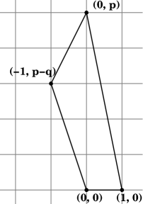
Figure 1: The fan of $C(Y^{p,q})$ for $p=5$, $q=2$.

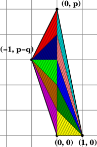
Figure 2: The fan of $\widetilde{C(Y^{p,q})}$ for $p=5$, $q=2$.

Figure 3: The $pq$-web diagram of $\widetilde{C(Y^{p,q})}$ for $p=5$, $q=2$.

The resolved geometry will be henceforth denoted as $\mathcal{X}_{p,q}\equiv\widetilde{C(Y^{p,q})}$ and the corresponding fan as $\Sigma_{p,q}$. It might also be described as a holomorphic quotient

$$(\mathbb{C}^{p+3}\setminus Z)/(\mathbb{C}^{*})^{p}$$

with $Z$ a co-dimension $>0$ locus determined by the toric data [16] and the $k^{th}$ $\mathbb{C}^{*}$ factor acting on the coordinates of $\mathbb{C}^{p+3}$ as $z_{i}\to\lambda^{Q^{(k)}_{i}}z_{i}$, where $Q_{i}^{(k)}\in\mathbb{Z}$ is a set of integers such that

$$\sum_{i=1}^{p+3}Q_{i}^{(k)}v_{i}=0\qquad k=1,\dots,p$$ (2.2)

The set of charges for $\mathcal{X}_{p,q}$ is given by (see fig. 2)

$$\begin{array}[]{ccccccccccccc}Q_{1}&=&(A,&-2A-B,&B,&A,&,0,&0,&0,&0,&0,&0,&0)\\ Q_{2}&=&(0,&1,&0,&0,&-2,&1,&0,&0,&\dots,&0,&0)\\ Q_{3}&=&(0,&0,&0,&0,&1,&-2,&1,&0,&\dots,&0,&0)\\ Q_{4}&=&(0,&0,&0,&0,&0,&1,&-2,&1,&\dots,&0,&0)\\ \vdots&&\vdots&\vdots&\vdots&\vdots&\vdots&\vdots&\vdots&\vdots&\vdots&\vdots&\vdots\\ Q_{p}&=&(0,&0,&1,&0,&0,&0,&0,&0,&\dots,&1,&-2)\end{array}$$ (2.3)

with $A$ and $B$ coprime numbers solving the Diophantine equation $(p-q)A+pB=0$ for $q<p$, while $A=1$ and $B=0$ for $q=p$. In real polar coordinates ($|z_{i}|,\theta_{i}$), this corresponds to the Higgs branch of a $\mathcal{N}=(2,2)$ $d=2$ gauged linear $\sigma$-model (GLSM) [18] with $p+3$ chiral fields $z_{i}$. The $D-$term equation of motion is

$$\sum_{j=1}^{p+3}Q_{j}^{k}|z_{i}|^{2}=t_{k}\qquad k=1,\dots,p$$ (2.4)

and $U(1)^{p}$ acts as

$$z_{j}\to e^{2\pi iQ_{j}^{(k)}\theta_{j}}z_{j}\qquad k=1,\dots,p$$ (2.5)

where $\theta_{j}=\hbox{arg}(z_{j})$. The Fayet-Iliopoulos parameters $t_{k}$ are complexified Kähler parameters of $\mathcal{X}_{p,q}$. Indeed, the full cohomology ring of the smooth $CY$ manifold thus obtained can be easily read off from the fan [16, 19]. For example, Betti numbers are

$$b_{0}=1\qquad b_{2}=p\qquad b_{4}=p-1\qquad b_{6}=0$$ (2.6)

Various aspects of these geometries have been considered in the context of topological strings. First of all, notice from figure 2-3 and formula (2.6) that for $p=1$ we encounter the two most studied local curves: the conifold $(q=0)$ and $\mathbb{C}\times K_{\mathbb{P}^{1}}$ ($q=1$), whose enumerative geometry [20], phase structure [21] and local mirror symmetry properties [22] have been extensively studied. For $p=2$, the local $CY$ in question is the total space of the canonical line bundle $K_{\mathbb{F}_{q}}$ over the $q^{th}$ Hirzebruch surface, $q=0,1,2$. For higher $p$ we have the ladder geometries considered in [23, 24, 25, 11] in the context of geometric engineering of pure $SYM$ theories with eight supercharges. In a suitable field theory limit described in [23], the Gromov-Witten large radius expansion for these geometries was shown to reproduce for all $q$ the weak coupling instanton expansion of the prepotential for $\mathcal{N}=2$ $SU(p)$ pure Yang-Mills in $d=4$. Subsequently, they were shown [10, 9, 26], to geometrically engineer $\mathcal{N}=1$ $SU(p)$ $SYM$ on $\mathbb{R}^{4}\times S^{1}$ with Chern-Simons coupling $k=p-q$, with the field theory limit above interpreted now as the limit in which the fifth-dimensional circle shrinks to zero size.
The Kähler moduli space of these geometries presents a manifold richness of phenomena which provide a natural testing ground for $A$-twisted topological string theory away from the large radius phase, as well as for the search of direct evidence for open/closed dualities in the strongly coupled $\alpha^{\prime}$ regime. The pivotal example of the latter is given by the case $q=0$, which is the large $N$ dual background of the open $A$-model on $T^{*}L(p,1)$ obtained via geometric transition [27]. Moreover, it was noticed in [14, 19] that $\mathcal{X}_{p,q}$ can be “blown-down” to orbifolds of flat space of the form $\mathbb{C}^{3}/\mathbb{Z}_{p+q}$ (see table 1); here the geometric picture becomes singular, though leaving still open the possibility for extracting enumerative results in terms of orbifold Gromov-Witten invariants. These are precisely the cases we will turn to study in section 4.

$p$	$q$	$p+q$	Weights
$1$	$0$	$1$	$(0,0,0)$
$1$	$1$	$2$	$(0,1,1)$
$2$	$0$	$2$	$(0,1,1)$
$2$	$1$	$3$	$(1,1,1)$
$2$	$2$	$4$	$(1,1,2)$

Table 1: Orbifold degenerations of $\mathcal{X}_{p,q}$ into $\mathbb{C}^{3}/\mathbb{Z}_{p+q}$ for the first few values of $p$ and $q$. The fourth column lists the weights of the $\mathbb{Z}_{p+q}$ action on the coordinates $(z_{1},z_{2},z_{3})$ of $\mathbb{C}^{3}$.

3 Mirror symmetry for local CY and integrable systems

3.1 Period integrals

A procedure for constructing mirror duals of (among others) toric $CY$ threefolds has been provided in [28], elaborating on previous results of [29, 30]. The mirror geometry $\widehat{\mathcal{X}_{p,q}}$ of $\mathcal{X}_{p,q}$ is an affine hypersurface in $\mathbb{C}^{2}\times(\mathbb{C}^{*})^{2}$

$$x_{1}x_{2}=H_{p,q}(u,v)$$ (3.1)

with $(x_{1},x_{2})\in\mathbb{C}^{2}$ and $(u,v)\in(\mathbb{C}^{*})^{2}$. In (3.1) $H_{p,q}(u,v)$ is the Newton polynomial [31] of the polytope $\Sigma_{p,q}\cap\{r_{3}=1\}$ in $\mathbb{Z}^{3}$ given by the intersection of the fan with the affine hyperplane $r_{3}=1$

$$H_{p,q}(u,v)=a_{1}v+\frac{a_{2}u^{p-q}}{v}-\sum_{i=0}^{p}a_{i+3}u^{i}$$ (3.2)

The geometry is therefore that of a quadric fibration over the $H_{p,q}(u,v)=\lambda\in\mathbb{C}$ plane, which degenerates to a node above the punctured Riemann surface $H_{p,q}(u,v)=0$. We will call the latter the mirror curve $\Gamma_{p,q}$.
Now, mirror symmetry in the compact case prescribes to reconstruct the A-model prepotential from the computation of the (properly normalized) periods of the holomorphic $(3,0)$ form $[\Omega]\in H^{3,0}(\widehat{\mathcal{X}_{p,q}})$ on a symplectic basis of homology three-cycles

$$\vec{\Pi}=\int_{\vec{\Gamma}\in H_{3}(\widehat{\mathcal{X}_{p,q}},\mathbb{Z})}\Omega$$

where $\Omega$ in this case would be the residue form on $H_{p,q}=0$ of the holomorphic $4$-form in $H^{4,0}(\mathbb{C}^{2}\times(\mathbb{C}^{*})^{2}\setminus\widehat{\mathcal{X}_{p,q}})$

$$\Omega=\hbox{Res}_{H_{p,q}(u,v)=x_{1}x_{2}}\left[\frac{dx_{1}dx_{2}du/udv/v}{x_{1}x_{2}-H_{p,q}(u,v)}\right]$$ (3.3)

Special geometry then ensures [32] that the periods are related as

$$\vec{\Pi}=(t_{0}(a),t_{i}(a),\partial_{t_{i}}\mathcal{F}(a),2\mathcal{F}-\sum_{i}t_{i}\partial_{t_{i}}\mathcal{F})$$ (3.4)

where $t_{i}(a)$ defines a local isomorphism between the A model moduli space of $\mathcal{X}_{p,q}$ and the B model moduli space of $\widehat{\mathcal{X}_{p,q}}$, while $\mathcal{F}(t)$ is the prepotential, i.e. the sphere amplitude. They have respectively single and double logarithmic singularities at the large complex structure point [29]. In the local case under scrutiny we must actually cope with the absence of a symplectic basis for $H_{3}(\widehat{\mathcal{X}_{p,q}},\mathbb{Z})$; according to [33, 22], the formalism carries through to the local setting by considering non-compact cycles as well and defining the periods along them via equivariant localization. We will denote the corresponding extended homology as $H_{3}^{(ext)}(\widehat{\mathcal{X}_{p,q}},\mathbb{Z})$.
The usual procedure the $(t_{i},\partial_{i}\mathcal{F})$ are found is via integration of the associated $GKZ$ hypergeometric system [32, 29]

$$\prod_{Q_{i}^{(k)}>0}\left(\frac{\partial}{\partial a_{i}}\right)^{Q_{i}^{(k)}}=\prod_{Q_{i}^{(k)}<0}\left(\frac{\partial}{\partial a_{i}}\right)^{Q_{i}^{(k)}}\qquad k=1,\dots,p$$ (3.5)

with $Q_{i}^{(k)}$ as in (2.3). In a patch of the B-model moduli space, these are the Picard-Fuchs ($PF$) equations for $\widehat{\mathcal{X}_{p,q}}$. Typically, solutions of (3.5) are obtained via series integration by Frobenius method, i.e. solving recursion relations for the coefficients of a series expansions for $(t_{i},\partial_{i}\mathcal{F})$. This has to be done patch by patch in the moduli space though, and it turns out to be hardly practicable as soon as the number of Kähler classes increases. To our knowledge, there is no explicit solutions in the literature when $h_{11}(\mathcal{X}_{p,q})>2$.
A possible alternative way to find $\vec{\Pi}$ is via direct integration. This not viable in the general case, but notice that due to the particular form (3.1) of $\widehat{\mathcal{X}_{p,q}}$, the integration of $\Omega$ over three-cycles boils down to that of a $1$-differential $d\lambda$ over a basis of cycles in $H_{1}^{(ext)}(\Gamma_{p,q},\mathbb{Z})$. As shown in [22], the periods of $\Omega$ solve the $PF$ system (3.5) if and only if those of

$$d\lambda_{p,q}\equiv\hbox{Res}_{H_{p,q}(u,v)=0}\left[\frac{dudv}{uv}\log{H_{p,q}(u,v)}\right]$$ (3.6)

do on a basis of $H_{1}^{(ext)}(\Gamma_{p,q},\mathbb{Z})$. Picking up the residue gives

$$d\lambda=\log{v}\frac{du}{u}$$ (3.7)

and the periods are thus computed as

$$\Pi^{\Gamma_{p,q}}_{\gamma}=\int_{\gamma\in H_{1}^{(ext)}(\Gamma_{p,q},\mathbb{Z})}\log{v}\frac{du}{u}$$ (3.8)

Unfortunately, the integrals are typically too awkward to carry out and no expression is known except for the simplest case of local curves; a perturbative evaluation of them, though clearly possible, has no real advantages compared to tackling the $PF$ system upfront. However, we will see in section 4 how to handle them in a direct way.

3.1.1 Mirror symmetry for open strings

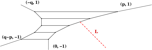
Figure 4: The pq-web for $p=5$, $q=2$ with a lagrangian brane on an inner leg.

Recently, the open string sector of the $A$-model on toric $CY$ has been subject to deeper investigation, following the insight of [34, 35], where a class of special Lagrangian submanifolds was constructed generalizing [36]. The prescription of [34] relies on the realization of a toric $CY$ as a (degenerate) $\mathbb{T}^{3}$ fibration, parameterized by $\theta_{i}$, over the $|z_{i}|$ base, see (2.4, 2.5). The authors of [34] consider a $3-k$ real dimensional linear subspace $W$ of the base

$$\sum_{i}q_{i}^{\alpha}|z_{i}|^{2}=c^{\alpha}\qquad\alpha=1,\dots,k;\quad q_{i}^{\alpha}\in\mathbb{Q}$$ (3.9)

and then specify a $\mathbb{T}^{k}$ fibration $L$ over this subspace in such a way that the Kähler form $\omega=\sum_{i}d|z_{i}|^{2}\wedge d\theta_{i}$ vanishes on it

$$\omega|_{L}=0$$ (3.10)

The total space of this fiber bundle $L$ is then Lagrangian by construction; moreover, it turns out that it is volume minimizing in its homology class (special Lagrangian) if and only if $\sum_{i}q_{i}^{\alpha}=0$. In this case (3.10) implies

$$\sum_{i}\theta_{i}=0$$ (3.11)

In the case in which $c^{\alpha}$ in (3.9) are such that $W$ intersects the edges of the toric web, i.e. the loci where one $S^{1}$ of the toric fibration shrinks, $L$ splits into two Lagrangians $L_{\pm}$ with topology $\mathbb{R}^{2}\times S^{1}$: the open modulus $z$ is then given by the size of the circle, complexified with the holonomy of a $U(1)$ connection along it.
The mirror symmetry construction of [28] has been extended to these brane configurations in [34]. When $k=2$, $L_{+}$ (resp. $L_{-}$) gets mirror mapped to a curve parameterized by $x_{2}$ (resp. $x_{1}$)

$$H_{p,q}(u,v)=0=x_{1}\quad(\hbox{resp.}=x_{2})$$ (3.12)

The moduli space of the mirror brane is then simply the mirror curve $\Gamma_{p,q}$. Picking a parametrization thereof (for instance the projection on the $u$ or $v$-lines) by a complex variable $z$ leads us to write the open topological partition function

$$\mathcal{F}_{open}(\{t_{i}\},z)=\sum_{g,h}\mathcal{F}_{g,h}(\{t_{i}\})z^{h}$$ (3.13)

the sum is both over the genus of the source curve and the number of connected components of its boundary. The choice of a “good” parametrization is dictated by mirror symmetry and is related to phase transitions in the open string moduli space for branes ending on toric curves meeting at a vertex in the web (see [8] for details).
A very important fact is that the meromorphic differential $d\lambda$ turns out to have a significant role for open string amplitudes as well. The dimensional reduction of the holomorphic Chern-Simons action on the mirror brane indeed yields a particularly simple expression for the disc amplitude $g=0$, $h=1$. It is simply given by the “Abel-Jacobi” map

$$\mathcal{F}_{0,1}(t,z)=\int^{z}\log{v(u)}\frac{du}{u}$$ (3.14)

where the integral on the r.h.s. is a chain integral $[z^{*},z]$, with $z^{*}$ a fixed point on the mirror curve. In [37] it was noticed that the disc amplitude (3.14) in a suitable parameterization gets the form

$$\mathcal{F}_{0,1}(t,z_{open})=\sum_{m,n}N_{m,n}Li_{2}(e^{-t\cdot m}z_{open}^{n})$$ (3.15)

In (3.15) $N_{m,n}$ are integer numbers counting open string BPS states and $z_{open}$ is the dressed open coordinate [35]

$$z_{open}=z+\sum_{i}\frac{w_{i}-t_{i}}{r_{i}}$$ (3.16)

where $w_{i}$ are combinations of gauge-invariant sigma model variables vanishing at the point of maximally unipotent monodromy

$$w_{i}=\prod_{j}a_{j}^{Q_{j}^{(i)}}=t_{i}+\mathcal{O}(e^{-t_{i}})$$ (3.17)

and $r_{i}$ are rational numbers. Notice that the open flat coordinates gets corrected by closed worldsheet instantons only. As discovered in [38],(see also [39]) an extended Picard-Fuchs system may be constructed such that (3.14), (3.16) are in its kernel and this can be used for determining the $r_{i}$ in (3.16).

3.2 The $B$-model moduli space

A few remarks are in order at this point. The Riemann surfaces $\Gamma_{p,q}$ come in a family parameterized by $\{a_{i}\}$ in (3.1), which are the complex moduli of the mirror geometry. The curve $\Gamma_{p,q}$ will be generically smooth in the $B$-model moduli space: we will denote the open set where this happens as $\mathcal{M}^{B}_{p,q}$. However, a compactification of $\mathcal{M}^{B}_{p,q}$ will lead to loci where this is no longer true. Indeed, $\Gamma_{p,q}$ degenerates to a singular curve on the so-called principal discriminant locus of the $PF$ system (3.5). In correspondence with this, one of the homology cycles of $\Gamma_{p,q}$ shrinks to zero size; $GKZ$ solutions have then singularities and are subject to logarithmic monodromy transformations around these loci, to which we will refer to as conifold loci. Moreover, there also regions in the $B$-model moduli space where the curve $\Gamma_{p,q}$ stays smooth, but the periods have finite monodromy because the moduli space itself is singular, locally looking like $\mathbb{C}^{p}/\mathbb{Z}_{n}$; at the conformal field theory level, this would be reflected by the appearance of a discrete quantum symmetry. We will refer to the latter as an orbifold phase, in which we still retain a geometric picture, though involving a singular (orbifold) target space in the $A$-model side.
To see why this happens from the mirror perspective one might argue as follows. The $a_{i}$’s are sort of homogeneous coordinates for the complex structure moduli space of $\widehat{\mathcal{X}^{p,q}}$. Indeed, only $p$ out of $p+3$ are really independent, as an overall rescaling of them and scalings of $u$ and $v$ in (3.1) leave invariant the symplectic form

$$\frac{du}{u}\wedge\frac{dv}{v}$$ (3.18)

in $(\mathbb{C}^{*})^{2}$. That is, the moduli space of the mirror theory might be seen as arising from a holomorphic quotient of $\mathbb{C}^{p+3}$ by a $(\mathbb{C}^{*})^{3}$ action with charges (see (3.2))

$$\begin{array}[]{c|cccccccc}&a_{1}&a_{3}&a_{p+3}&a_{2}&a_{4}&\dots&a_{p+2}\\ \hline\cr Q_{1}&1,&0,&0,&-1,&0,&\dots,&0\\ Q_{2}&0,&0,&p,&p-q,&1,&\dots,&p-1\\ Q_{3}&1,&1,&1,&1,&1,&\dots,&1\\ \end{array}$$ (3.19)

By subtracting a suitable codimension $>0$ locus to $\mathbb{C}^{p+3}$, we thus end up with a toric compactification of the family $\mathcal{M}^{B}_{p,q}$, which we call $\overline{\mathcal{M}^{B,tor}_{p,q}}$. Remarkably enough, inspection shows [32] that the skeleton of a fan for the above system of charges is simply given by the columns of the $GLSM$ (2.3), and the toric variety associated with it is complete. This fan is called the secondary fan of $\mathcal{X}^{p,q}$. In fact, strictly speaking we are not dealing with a toric variety, as typically the secondary fan will contain non-smooth simplicial cones, perhaps with marked points along their facets. In the latter case, this would mean that the patch parameterized by the corresponding $a_{i}$’s looks like $\mathbb{C}^{p}/\mathbb{Z}_{n}$ rather than $\mathbb{C}^{p}$; as such, the periods of the holomorphic three-form will inherit the finite monodromy from the monodromy of the $a_{i}$ themselves. This will be of fundamental importance in our study of the $[\mathbb{C}^{3}/\mathbb{Z}_{4}]$ orbifold in section 4.
Additional, but somewhat milder phase transitions involve the purely open string sector as well and are related, as already anticipated, to a choice of a parametrization of $\Gamma_{p,q}$. See [8], to which we refer for a complete discussion of this subject.

3.3 Relation with integrable systems and five-dimensional gauge theories

Interestingly, the mirror curves of $\mathcal{X}_{p,q}$ geometries are related to the Seiberg-Witten curve of five dimensional gauge theories and the related integrable systems. Since, as we will show in the next section, this observation will prove to be very fruitful in the study of the topological string moduli space of $\mathcal{X}_{p,q}$, we describe it here in some detail.
First of all, let us rewrite (3.2) as

$$Y^{2}=P_{p}(X)^{2}-4a_{1}a_{2}X^{p-q}$$ (3.20)

upon setting

$$Y=a_{1}v-a_{2}u^{p-q}/v$$

$$X=u$$

$$P_{p}(X)=\sum_{i=0}^{p}a_{i+3}X^{i}$$ (3.21)

In the $a_{1}=a_{2}=(\Lambda R)^{p}$, $a_{3}=a_{p}=1$ patch the curve (3.20) and the differential (3.7) are precisely the Seiberg-Witten curve and differential of $SU(p)$ ${\cal N}=1$ SYM theory on $\mathbb{R}^{4}\times S^{1}$ with a $q$-dependent Chern-Simons term [11, 26].

Moreover, the SW curve and differential in the case $p=q$ were shown in [40] to coincide with the spectral curve and action differential of the $A_{p-1}$ Ruijsenaars model [12], i.e. the $A_{p-1}$ periodic relativistic Toda chain. More precisely, setting $\zeta=\Lambda R$, (3.2) reads for $p=q$

$$\Gamma_{p,p}:\quad\zeta^{p}(v+\frac{1}{v})=1+\sum_{l=1}^{p-1}u^{l}S_{l}+u^{p},\quad d\lambda_{p,p}=\log{v}\frac{du}{u}$$

which can be rewritten as

$$\det(L(z)-w)=\sum_{j=0}^{p}(-w)^{p-j}\sigma_{j}(z)=0$$ (3.22)

with the Lax matrix defined as

$$L_{ij} = e^{Rp_{i}}f_{i}(l_{ij}+b_{ij})$$

$$l_{ij} = \delta_{i,j+1}(1+\zeta^{p}z)\xi_{i}-\delta_{i,1}\delta_{j,p}(1+\zeta^{-p}z^{-1})\xi_{1}$$

$$b_{ij} = \Biggl{[}\begin{array}[]{cc}-(i\zeta)^{p}&\quad i\leq j-1\\ 1&\quad i>j-1\end{array}$$ (3.25)

$$f_{i}^{2} = (1-\zeta^{2}e^{q_{i+1}-q_{i}})(1-\zeta^{2}e^{q_{i}-q_{i-1}})$$

$$\xi_{i}^{-1} = 1-\zeta^{-2}e^{q_{i-1}-q_{i}}$$ (3.26)

where $q_{p+1}=q_{1},q_{0}=q_{p}$, $\sigma_{j}$ are the elementary symmetric functions of $L(z)$, $S_{j}$ their $z$-independent factor, and we have made the change of variables [40]

$$-wu=1+\zeta^{p}z,\quad z=v$$

An identification of the curves for $q<p$ as the spectral curves of some finite dimensional integrable mechanical system seems to be presently not known, and it would be interesting to understand to role of the $q$ parameter in this context.

A second important remark is about the “field theory limit” discussed in [23]. From the mechanical system point of view, the parameter $\zeta$ in (3.26) is essentially the inverse of the speed of light, while in the field theory perspective $\zeta=\Lambda R$, where $\Lambda$ is the strong coupling scale and $R$ is the radius of the fifth-dimensional circle. This means that the four-dimensional limit might be achieved as the non-relativistic limit of the Toda chain. Denoting with $e^{\phi_{i}}$, $i=1\dots,p$ the roots of the polynomial $P_{p}(x)$ (3.21) and introducing the new set of variables [11]

$$y = Y$$

$$X = e^{2Rx}$$ (3.27)

$$e^{\phi_{i}} = e^{R(a_{i}-a_{i+1})}$$

we have that in the $R\to 0$ limit (3.20) reduces to

$$y^{2}=\tilde{P}_{p}(x)^{2}-4\Lambda^{2p}$$ (3.28)

which is the Seiberg-Witten curve of $\mathcal{N}=2$ $SU(p)$ Super Yang-Mills in $d=4$. Notice that in the $R\to 0$ limit we completely lose track of the Chern-Simons parameter $q$, which has disappeared in formula (3.28). More importantly, the variable $x$ in (3.3) takes now values in $\mathbb{C}$ in contrast with the $\mathbb{C}^{*}-$variable $X$. Because of this, the peculiarly five-dimensional form of the differential (3.7), i.e. $d\lambda=\log{v}d\log{u}$, is replaced in the $R\to 0$ limit by that of the usual (non-relativistic) Toda differential $d\lambda=xd\ln(\tilde{P_{p}}+y)$. In fact, as we will see in the following, the relativistic system and its non-relativistic counterpart - which by the discussion above coincide respectively with the $A-$model on $\mathcal{X}_{p,q}$ and with its $4d$ Seiberg-Witten limit - bear still deep structural resemblances and our aim will be to try to exploit this to our advantage.

4 Solving the $GKZ$ system in the full moduli space

In this section we provide a method for finding the mirror map, as well as the sphere and disc amplitude, for the $A$-model on $\mathcal{X}_{p,q}$ to all orders in $\alpha^{\prime}$ without resorting to solving the $GKZ$ system directly. This will be accomplished by finding closed forms for derivatives of the period integrals $\Pi^{\Gamma_{p,q}}_{\gamma}$ w.r.t. the bare moduli as generalized hypergeometric functions.

First of all, let us resume what the ingredients at our disposal are. According to (3.20) the mirror curve $\Gamma_{p,q}$ is a two-fold covering of the $X$ plane branched at $Y(X)=0$, that is the locus

$$P_{p}(X)^{2}=4a_{1}a_{2}X^{p-q}$$ (4.1)

The resulting curve has genus $p-1$ and four punctures corresponding to the two inverse images of $X=0$, $X=\infty$. Let us denote the solutions to (4.1) as $\{b_{i}\}_{i=1}^{2p}$. A basis for $H_{1}^{(ext)}(\Gamma_{p,q},\mathbb{Z})$ might be taken as the circles $A_{i}$, $B_{i}$ encircling the intervals

$$I_{A_{i}}=[b_{2i-1},b_{2i}]\qquad I_{B_{i}}=[b_{2i},b_{2i+1}]$$ (4.2)

for $i=1,\dots,p-1$, plus a circle $A_{0}$ around one of the punctures at $X=0$ and a contour $B_{0}$ connecting the two punctures at $X=0$ and $X=\infty$.

Figure 5: Cuts and punctures of the $X$ plane in the genus $1$ case.

The 1-differential $d\lambda_{p,q}$ is given, in an affine patch parameterized by $X$, as

$$d\lambda_{p,q}(X)=\log v(u)\frac{du}{u}=\log\left(\frac{P_{p}(X)\pm\sqrt{P_{p}(X)^{2}-4a_{1}a_{2}X^{p-q}}}{2a_{1}}\right)\frac{dX}{X}$$ (4.3)

and a complete set of periods can be obtained by integrating it over the $A/B$-cycles

$$\Pi_{A/B}=\oint_{A/B}d\lambda_{p,q}$$ (4.4)

More explicitly,

$$\Pi_{A_{i}} = \int_{b_{2i-1}}^{b_{2i}}\log\left(\frac{P_{p}(X)+\sqrt{P_{p}(X)^{2}-4a_{1}a_{2}X^{p-q}}}{P_{p}(X)-\sqrt{P_{p}(X)^{2}-4a_{1}a_{2}X^{p-q}}}\right)\frac{dX}{X}$$ (4.5)

$$\Pi_{B_{i}} = \int_{b_{2i}}^{b_{2i+1}}\log\left(\frac{P_{p}(X)+\sqrt{P_{p}(X)^{2}-4a_{1}a_{2}X^{p-q}}}{P_{p}(X)-\sqrt{P_{p}(X)^{2}-4a_{1}a_{2}X^{p-q}}}\right)\frac{dX}{X}$$ (4.6)

$$\Pi_{A_{0}} = \oint_{X=0}\log\left(\frac{P_{p}(X)\pm\sqrt{P_{p}(X)^{2}-4a_{1}a_{2}X^{p-q}}}{2a_{1}}\right)\frac{dX}{X}$$ (4.7)

$$\Pi_{B_{0}} = \int_{0}^{\infty}\log\left(\frac{P_{p}(X)\pm\sqrt{P_{p}(X)^{2}-4a_{1}a_{2}X^{p-q}}}{2a_{1}}\right)\frac{dX}{X}$$ (4.8)

We now make the following observation. As we have already noticed, the curve (3.20) and the differential (4.3) are the Seiberg-Witten (SW) curve and differential of a five dimensional theory compactified on a circle. In Seiberg-Witten theory, the gauge coupling matrix

$$\tau_{ij}=\frac{\partial\Pi_{B_{i}}}{\partial u_{k}}\left(\frac{\partial\Pi_{A_{k}}}{\partial u_{j}}\right)^{-1}$$ (4.9)

where $u_{i}$ are Weyl-invariant functions of the scalar fields, is known to be the period matrix of the compactified SW curve, that is a ratio of periods of holomorphic differentials. We then expect that derivatives of $d\lambda_{p,q}$ with respect to suitable functions of the bare moduli are holomorphic differentials on the compactified $\overline{\Gamma}_{p,q}$

$$[\partial_{f(a_{i})}d\lambda]\in H^{1,0}(\overline{\Gamma}_{p,q})$$ (4.10)

This is substantiated by the fact that, for $p=q=2$, the relativistic Toda system and the non-relativistic one share the same oscillation periods [41]; more precisely, the derivatives of the action with respect to the energy are the same (elliptic) functions of the bare parameters. This was also noticed in [40] in the study of the singularities of the moduli space of $\mathcal{N}=1$ $SU(2)$ $SYM$ in $d=5$.
Explicitly, we indeed have

$$\frac{\partial d\lambda_{p,q}}{\partial a_{j+4}}=\frac{X^{j}}{\sqrt{P^{2}_{p}(X)-4a_{1}a_{2}X^{p-q}}}dX$$ (4.11)

i.e., for $j=0,\dots,p-2$, a basis of holomorphic $1$-forms on the $4$-point compactification $\overline{\Gamma}_{p,q}=\Gamma_{p,q}\cup\{0_{+},0_{-},\infty_{+},\infty_{-}\}$ of the spectral curve $\Gamma_{p,q}$.

4.1 Period integrals and Lauricella functions

This last observation allows us to give a straightforward recipe for computing series expansions of solutions of the $GKZ$ system (3.5) in the full $B$-model moduli space. The procedure is the following:

1. start with $\Pi_{A_{i}/B_{i}}$ and consider its $a_{j+4}$ derivative for $0\leq j\leq p-2$

   $$\frac{\partial\Pi_{A_{i}/B_{i}}}{\partial a_{j+4}}=\int_{e_{i}}^{e_{i+1}}\frac{X^{j}}{\sqrt{\prod_{i=1}^{2p}(X-b_{i})}}dX$$ (4.12)

   with $e_{i}=b_{2i-1}$, $e_{i}=b_{2i}$ for the $A$ and the $B$ cycles respectively. The hyperelliptic integral (4.12) has a closed expression given in terms of multivariate generalized hypergeometric functions of Lauricella type [42]

   $$\frac{\partial\Pi_{A_{i}/B_{i}}}{\partial a_{j+4}} = {\rm e}^{i\varphi}\pi\frac{(e_{i})^{j}}{\sqrt{\prod_{k\neq i,i+1}(e_{k}-e_{i})}}$$

   $$\times F_{D}^{(2p-1)}\left(\frac{1}{2};\frac{1}{2},\dots,\frac{1}{2},j;1;x_{1},\dots,\widehat{x_{i}},\widehat{x_{i+1}},\dots,x_{2p},\frac{e_{i+1}-e_{i}}{e_{i}}\right)$$

   where $x_{j}=(e_{i+1}-e_{i})/(e_{j}-e_{i})$, $2\varphi=l\pi$, $l\in\mathbb{Z}$ is a phase depending on $x_{i}$ and $F_{D}^{(n)}$ is the hypergeometric series

   $$F_{D}^{(n)}(\alpha;\{\beta_{i}\};\gamma;\{\delta_{i}\})=\sum_{m_{1}\dots m_{n}=0}^{\infty}\frac{(\alpha)_{m_{+}\dots+m_{n}}(\beta_{1})_{m_{1}}\dots(\beta_{n})_{m_{n}}\delta_{1}^{m_{1}}\dots\delta_{n}^{m_{n}}}{(\gamma)_{m_{+}\dots+m_{n}}m_{1}!\dots m_{n}!}$$ (4.14)

   which converges when $|\delta_{i}|<1$ for every $i$. In the above formula we used the standard Pochhammer symbol $(\alpha)_{m}=\Gamma(\alpha+m)/\Gamma(\alpha)$. There are many alternative ways to express (4.12), for instance in terms of hyperelliptic $\theta$ functions; however, the above expression proves to be useful due to the fact that Lauricella $F_{D}^{(n)}$ has good analytic continuation properties outside the unit polydisc $|\delta_{i}|<1$; some formulae, as well as asymptotic expansions around singular submanifolds, are collected in the Appendix, while others can be found in [42, 43]. Notice that, as opposed to the usual situation in solving $PF$ equations by Frobenius method, we are not dealing here with hypergeometric functions of the bare moduli, but rather of the relative distance $x_{i}$ between ramification points; they have singular values precisely when the latter becomes $0$, $1$ or infinity, that is when we encounter a pinching point of $\Gamma_{p,q}$. This shift in perspective is definitely an advantage compared to other expressions for hyperelliptic integrals, involving for instance the $F_{4}$ Appell function for genus 2 [44, 45]. These are simpler functions of the bare moduli, but have worse analytic continuation properties and are less suited for a more complete study of the moduli space, regarding for instance intersecting submanifolds of the principal discriminant locus. The above fact was already pointed out in [46], where the properties of $F_{D}^{n}$ were exploited to study the $\mathbb{Z}_{3}$ point of $\mathcal{N}=2$ $SU(3$) $SYM$.
   In many cases, $F_{D}^{(n)}$ can be reduced to a more familiar form. For instance, for $p=2$ we have the expected complete elliptic integrals of the first kind

   $$\frac{\partial\Pi_{A}}{\partial a_{4}} = \frac{2}{\sqrt{(b_{1}-b_{3})(b_{2}-b_{4})}}K\left[\frac{(b_{1}-b_{2})(b_{3}-b_{4})}{(b_{1}-b_{3})(b_{2}-b_{4})}\right]$$ (4.15)

   $$\frac{\partial\Pi_{B}}{\partial a_{4}} = \frac{2}{\sqrt{(b_{1}-b_{2})(b_{3}-b_{4})}}K\left[\frac{(b_{1}-b_{3})(b_{2}-b_{4})}{(b_{1}-b_{2})(b_{3}-b_{4})}\right]$$ (4.16)

2. Once we have a representation for the derivatives of the periods in the form (1), (4.15)-(4.16) we can use the formulae in Appendix B to analytically continue them in any given patch of the $B$-model moduli space and find a corresponding power series expansion in the bare moduli $a_{i}$. Integrating back with respect to $a_{j}$ yields $\Pi_{A_{i}}$ and $\Pi_{B_{i}}$ up to a constant of integration, independent of $a_{j}$ for $0\leq j\leq p-2$. This has to be fixed either by some indirect consideration (for instance, by imposing a prescribed asymptotic behavior around a singular point) or by plugging it inside the $PF$ system and imposing that the period be in the kernel of the $GKZ$ operators. This operation leads to a closed $ODE$ integrable by quadratures, which completes the solution of the problem of finding expansions for $\Pi_{A_{i}/B_{i}}$ everywhere in the $B$-model moduli space.

3. The procedure provides us with $p-1$ flat coordinates as well as $p-1$ conjugate periods out of which to extract the prepotential. In order to find the $p^{th}$ modulus, we pick up the residue (4.7)

   $$\oint_{X=0_{\pm}}d\lambda=\left\{\begin{array}[]{cc}\log\left(\pm\frac{a_{3}}{a_{1}}\right)&\hbox{for }q<p\\ \log\left(\frac{a_{3}\pm\sqrt{a_{3}^{2}-4a_{1}a_{2}}}{2a_{1}}\right)&\hbox{for }q=p\end{array}\right.$$ (4.17)

   which are manifestly solutions of (3.5). In the following, we will choose an appropriate combination of them in order to have a prescribed behavior around the expansion point under scrutiny.

4. Closed form computation of derivatives with respect to $a_{j}$ can be done for open string amplitudes as well, which might be used to trade an expansion in terms of the $z$ parameter in (3.16) with one in $a_{j}$, completely resummed w.r.t. $z$. In this case, dealing with chain integrals instead of period integrals leads one to consider indefinite integrals and thus incomplete hyperelliptic integrals. The latter can still be given the form of a multivariate Lauricella function, but with order increased by one [42]

   $$\frac{\partial\mathcal{F}_{0,1}(\{a_{k}\},z)}{\partial a_{j+4}} = {\rm e}^{i\varphi}\pi\frac{(e_{i})^{j}}{\sqrt{\prod_{k\neq i,i+1}(e_{k}-e_{i})}}2\sqrt{z}$$

   $$\times F_{D}^{(2p)}\left(\frac{1}{2};\frac{1}{2},\dots,\frac{1}{2},j,\frac{1}{2};\frac{3}{2};x_{3},\dots,x_{2p},\frac{e_{2}-e_{1}}{e_{1}},z\right)$$

   As before, for $p=2$ (4) boils down to an incomplete elliptic integral of the first kind in the form

   $$\frac{\partial\mathcal{F}_{0,1}(\{a_{k}\},z)}{\partial a_{4}}=2\sqrt{\frac{1}{\tilde{b}}}F\left(\sin^{-1}\left(\sqrt{\frac{(b_{1}-b_{4})(b_{2}-z)}{(b_{2}-b_{4})(b_{1}-z)}}\right)\Bigg{|}\frac{\tilde{a}}{\tilde{b}}\right)$$ (4.19)

   where

   $$\tilde{a}=(b_{2}-b_{4})(b_{1}-b_{3})\qquad\tilde{b}=(b_{2}-b_{3})(b_{1}-b_{4})$$

Another important advantage of this method is that, instead of integrating back patch-wise with respect to $a_{j}$, we can get our hands dirty and work directly with an Euler-type integral representation of the periods. The fact that $F_{D}^{(n)}$ has a single integral representation saves us most of the pain in the problem of finding the explicit analytic continuation of $\Pi_{A_{i}/B_{i}}$, which in the multi-parameter case involves the use of multi-loop Mellin-Barnes integrals. The details for the case $p=q=2$ which will be of our interest later on for the computation of orbifold Gromov-Witten invariants are reported in Appendix A, where also a closed expression for the A-period can be found in terms of a generalized Kampé de Fériet hypergeometric function.

5 Warm-up tests of the formalism

Let us show how the steps described in Section 4.1 allow to quickly recover some known results about mirror symmetry for local surfaces.

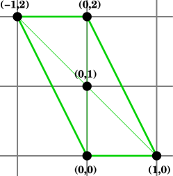
Figure 6: The fan of local $\mathbb{F}_{0}$.

5.1 Local $\mathbb{F}_{0}$ : mirror map at large radius

Local mirror symmetry for $K_{\mathbb{F}_{0}}$ has been studied in [47] in the check of the large $N$ duality with Chern-Simons theory on $S^{3}/\mathbb{Z}_{2}$. The mirror curve in this case can be written as

$$a_{1}v+a_{2}/v=a_{3}/u+a_{4}+a_{5}u$$ (5.1)

Good variables around the large complex structure point [29] are given by

$$z_{B}=\frac{a_{1}a_{2}}{a_{4}^{2}}\qquad z_{F}=\frac{a_{3}a_{5}}{a_{4}^{2}}$$ (5.2)

Let us use the scaling freedom (3.19) to set

$$a_{3}=a_{5}=1,\qquad a_{1}=a_{2}$$ (5.3)

By using the change of variables (3.20) the curve (5.1) is then given by

$$Y^{2}=\left(X^{2}+\frac{X}{\sqrt{z_{F}}}+1\right)^{2}-\frac{4z_{B}}{z_{F}}X^{2}$$ (5.4)

which is a double covering of the $X-$plane branched at

$$b_{1} = \frac{-1+2\sqrt{z_{B}}-\sqrt{1-4\sqrt{z_{B}}+4z_{B}-4z_{F}}}{2\sqrt{z_{F}}}$$ (5.5)

$$b_{2} = \frac{-1-2\sqrt{z_{B}}-\sqrt{1-4\sqrt{z_{B}}+4z_{B}-4z_{F}}}{2\sqrt{z_{F}}}$$ (5.6)

$$b_{3} = \frac{-1+2\sqrt{z_{B}}+\sqrt{1-4\sqrt{z_{B}}+4z_{B}-4z_{F}}}{2\sqrt{z_{F}}}$$ (5.7)

$$b_{4} = \frac{-1-2\sqrt{z_{B}}+\sqrt{1-4\sqrt{z_{B}}+4z_{B}-4z_{F}}}{2\sqrt{z_{F}}}$$ (5.8)

We choose the $A-$cycle as the loop encircling $[b_{1},b_{2}]$. The asymptotics of the corresponding period will indeed identify it as the flat coordinate around $z_{B}=z_{F}=0$. By expanding (4.15) in $(z_{B},z_{F})$ we have

$$\frac{\partial\Pi_{A}}{\partial a_{4}} = \sqrt{z_{F}}(20z_{B}^{3}+6(30z_{F}+1)z_{B}^{2}$$ (5.9)

$$+ 2(90z_{F}^{2}+12z_{F}+1)z_{B}+20z_{F}^{3}+6z_{F}^{2}+2z_{F}+1)+\dots$$

which integrates to

$$\Pi_{A}=\log(z_{F})+\frac{20z_{B}^{3}}{3}+60z_{F}z_{B}^{2}+3z_{B}^{2}+60z_{F}^{2}z_{B}$$ (5.10)

From (4.17) and (5.2) we can compute the remaining flat coordinate as

$$\Pi_{0}=-\frac{1}{2}\log\frac{z_{B}}{z_{F}}$$ (5.11)

It is then easy to see that the combinations of periods that has the right asymptotics at large radius are given by

$$-t_{B}\equiv-2\Pi_{0}(z_{B},z_{F})+\Pi_{A}(z_{B},z_{F}),\qquad-t_{F}\equiv\Pi_{A}(z_{B},z_{F})$$ (5.12)

Inversion of (5.10) and (5.11) reads, setting $Q_{B}=e^{-t_{B}}$, $Q_{F}=e^{-t_{F}}$

$$z_{B} = 6Q_{B}^{3}-2Q_{B}^{2}+6Q_{F}^{2}Q_{B}-2Q_{F}Q_{B}+Q_{B}+\dots$$

$$z_{F} = 6Q_{F}^{3}-2Q_{F}^{2}+6Q_{B}^{2}Q_{F}-2Q_{B}Q_{F}+Q_{F}+\dots$$ (5.13)

which is the mirror map as written in [48].

5.2 Local $\mathbb{F}_{0}$ : orbifold point

Analogously, we can write down the expansion for the orbifold point [47], which corresponds to $a_{1}=a_{2}=a_{3}=a_{5}=1$, $a_{4}=0$. Setting $a_{1}=a_{2}=\sqrt{1-x1}$, $a_{4}=x_{1}x_{2}$, $a_{3}=a_{5}=1$ as in [47], we have

$$s_{1} \equiv \Pi_{0}=-\log(1-x_{1})$$

$$s_{2} \equiv \Pi_{A}+\Pi_{B}/2=\frac{1}{61931520\pi}\bigg{[}x_{2}(35(32(x_{1}-2)x_{1}(x_{1}(11x_{1}-96)+96)E(x_{1})$$

$$+ x_{1}(x_{1}(x_{1}(x_{1}(105x_{1}-1856)+8000)-12288)+6144)K(x_{1}))x_{2}^{8}+\dots\bigg{]}$$

Upon introducing $\tilde{s}_{1}=s_{1}$ and $\tilde{s}_{2}=s_{1}/s_{2}$ we have

$$x_{1}(\tilde{s}_{1}) = 1-e^{-\tilde{s}_{1}}$$

$$x_{2}(\tilde{s}_{1},\tilde{s}_{2}) = \tilde{s}_{2}+\frac{\tilde{s}_{2}}{4}\tilde{s}_{1}+\bigg{(}\frac{\tilde{s}_{2}}{192}-\frac{\tilde{s}_{2}^{3}}{192}\bigg{)}\tilde{s}_{1}^{2}+\bigg{(}-\frac{\tilde{s}_{2}}{256}-\frac{\tilde{s}_{2}^{3}}{768}\bigg{)}\tilde{s}_{1}^{3}+\bigg{(}-\frac{49\tilde{s}_{2}}{737280}$$ (5.14)

$$+ \frac{7\tilde{s}_{2}^{3}}{73728}-\frac{7\tilde{s}_{2}^{5}}{245760}\bigg{)}\tilde{s}_{1}^{4}+\bigg{(}\frac{5\tilde{s}_{2}^{3}}{98304}-\frac{7\tilde{s}_{2}^{5}}{983040}\bigg{)}\tilde{s}_{1}^{5}+\dots$$

in perfect agreement with [47]. Needless to say, the prepotential computation can be checked exactly the same way. We have

$$F_{s_{2}}\equiv\Pi_{A} = \frac{1}{53760}\bigg{[}x_{1}x_{2}\Big{(}(75x_{1}^{3}x_{2}^{6}-56x_{1}^{2}(10x_{2}^{2}+9)x_{2}^{4}+64x_{1}(10x_{2}^{4}+21x_{2}^{2}$$ (5.15)

$$+ 70)x_{2}^{2}-107520\Big{)}K(1-x_{1})+\dots\bigg{]}$$

$$= \log\left(\frac{x_{1}}{16}\right)s_{2}-\frac{x_{2}^{3}}{12}x_{1}+(\frac{x_{2}}{4}+\frac{x_{2}^{3}}{48})x_{1}^{2}+\left(-\frac{21}{128}x_{2}+\frac{5}{768}x_{2}^{3}\right)x_{1}^{3}$$

$$+ \left(\frac{185x_{2}}{1536}+\frac{5x_{2}^{3}}{1024}\right)x_{1}^{4}+\dots$$

which reproduces the analogous formula in [47], modulo the ambiguity in the degree-zero contribution.

5.3 Local $\mathbb{F}_{2}$ at large radius

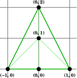
Figure 7: The fan of local $\mathbb{F}_{2}$.

We might proceed along the same lines for the case of local $\mathbb{F}_{2}$. The curve is given by

$$a_{1}v+\frac{a_{2}}{v}=a_{3}+a_{4}u+a_{5}u^{2}$$ (5.16)

Branch points are located at

$$u+\frac{a_{4}}{2a_{5}}=\left\{\begin{array}[]{c}\pm\frac{\sqrt{a_{4}^{2}-4a_{3}a_{5}-8\sqrt{a_{1}}\sqrt{a_{2}}a_{5}}}{2a_{5}}\equiv\pm c_{1}\\ \pm\frac{\sqrt{a_{4}^{2}-4a_{3}a_{5}+8\sqrt{a_{1}}\sqrt{a_{2}}a_{5}}}{2a_{5}}\equiv\pm c_{2}\end{array}\right.$$ (5.17)

and we have accordingly

$$\frac{\partial\Pi_{A}}{\partial a_{4}}=\int_{c_{1}}^{c_{2}}\frac{dX}{(X^{2}-c_{1}^{2})(X^{2}-c_{2}^{2})}=\frac{K\left(1-\frac{c_{2}^{2}}{c_{1}^{2}}\right)}{c_{1}}$$ (5.18)

$$\frac{\partial\Pi_{B}}{\partial a_{4}}=\int_{-c_{1}}^{c_{1}}\frac{dX}{(X^{2}-c_{1}^{2})(X^{2}-c_{2}^{2})}=\frac{2K\left(\frac{c_{1}^{2}}{c_{2}^{2}}\right)}{c_{2}}$$ (5.19)

In this case good coordinates associated to the base $\mathbb{P}^{1}$ and the $\mathbb{P}^{1}$ fiber are

$$z_{B}=\frac{a_{1}a_{2}}{a_{3}^{2}},\qquad z_{F}=\frac{a_{3}a_{5}}{a_{4}^{2}}$$ (5.20)

Upon setting $a_{1}=a_{2}$, $a_{3}=a_{5}=1$, periods take the form

$$\frac{\partial t_{F}}{\partial z_{F}} = \frac{\partial\Pi_{A}}{\partial z_{F}}=-\frac{2K\left(-\frac{16\sqrt{z_{B}}z_{F}}{-8\sqrt{z_{B}}z_{F}-4z_{F}+1}\right)}{\pi z_{F}\sqrt{1-4\left(2\sqrt{z_{B}}+1\right)z_{F}}}$$

$$\frac{\partial^{2}\mathcal{F}}{\partial z_{F}\partial t_{F}} = \frac{\partial\Pi_{B}}{\partial z_{F}}=-\frac{4K\left(\frac{-8\sqrt{z_{B}}z_{F}-4z_{F}+1}{8\sqrt{z_{B}}z_{F}-4z_{F}+1}\right)}{z_{F}\sqrt{1-4\left(1-2\sqrt{z_{B}}\right)z_{F}}}$$

$$t_{B} = \Pi_{0_{+}}-\Pi_{0_{-}}=2i\tan^{-1}\left(\sqrt{4z_{B}-1}\right)$$ (5.21)

where the normalization has been chosen in order to get the right asymptotics. Integration and inversion yields the mirror map at the large radius point

$$z_{B}(Q_{B}) = \frac{Q_{B}}{(Q_{B}+1)^{2}}$$

$$z_{F}(Q_{B},Q_{F}) = \left(1+Q_{B}\right)Q_{F}+\left(-2-4Q_{B}-2Q_{B}^{2}\right)Q_{F}^{2}$$ (5.22)

$$+ \left(3+3Q_{B}+3Q_{B}^{2}+3Q_{B}^{3}\right)Q_{F}^{3}+\dots$$

with $Q_{B}=e^{-t_{B}}$, $Q_{F}=e^{-t_{F}}$ and therefore

$$\partial_{t_{F}}\mathcal{F}(Q_{B},Q_{F}) = \left(\log(Q_{F})\log(Q_{B}Q_{F})\right)+\left(4+4Q_{B}\right)Q_{F}+(1+16Q_{B}+$$ (5.23)

$$+ Q_{B}^{2})Q_{F}^{2}+\left(\frac{4}{9}+36Q_{B}+36Q_{B}^{2}+\frac{4Q_{B}^{3}}{9}\right)Q_{F}^{3}$$

$$+ \left(\frac{1}{4}+260Q_{B}^{2}+64(Q_{B}+Q_{B}^{3})\right)Q_{F}^{4}+\dots$$

as in [29].

6 Local $\mathbb{F}_{2}$ and $[\mathbb{C}^{3}/\mathbb{Z}_{4}]$ orbifold Gromov-Witten invariants

6.1 Orbifold mirror map and genus zero invariants

We will now apply the considerations above to the study of the tip of the classical Kähler moduli space for local $\mathbb{F}_{2}$, where the compact divisor collapses to zero size. The resulting geometry [19] is a $\mathbb{Z}_{4}$ orbifold of $\mathbb{C}^{3}$ by the action $(\omega;z_{1},z_{2},z_{3})\to(\omega z_{1},\omega z_{2},\omega^{-2}z_{3})$, with $\omega\in\mathbb{Z}_{4}$. In the orbifold phase, the genus zero closed amplitude computes [49] the generating function of genus-zero correlators of twist fields

$$\mathcal{F}^{orb}(s_{1/4},s_{1/2})=\sum_{n,m}\frac{1}{n!m!}\langle\mathcal{O}_{1/4}^{m}\mathcal{O}_{1/2}^{n}\rangle s_{1/4}^{m}s_{1/2}^{n}$$ (6.1)

In (6.1) the sum is over the generators $s_{1/4}$, $s_{1/2}$ of the orbifold cohomology ring and they are associated respectively with the twisted sectors $1/4$ and $1/2$ under the $\mathbb{Z}_{4}$ action. The corresponding topological observables are denoted respectively as $\mathcal{O}_{1/4}$ and $\mathcal{O}_{1/2}$. The correlators $\langle\mathcal{O}_{1/4}^{m}\mathcal{O}_{1/2}^{n}\rangle$ compute genus-zero orbifold Gromov-Witten invariants $N^{orb}_{0,(m,n)}$ with $m$ insertions of weight $1/4$ and $n$ of weight $1/2$.

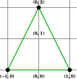
Figure 8: The fan of $[\mathbb{C}^{3}/\mathbb{Z}_{4}]$.

From figure 7 we see that Mori vectors for local $\mathbb{F}_{2}$ are

$$\begin{array}[]{ccccccc}Q_{1}&=&(0,&1,&1,&0,&-2)\\ Q_{2}&=&(1,&-2,&0,&1,&0)\end{array}$$ (6.2)

and the mirror curve $\Gamma_{2,2}$ has the form (5.16)

$$a_{1}v+\frac{a_{2}}{v}=a_{3}+a_{4}u+a_{5}u^{2}$$

Following [50] we argue that the point we are looking for in the $B$-model moduli space is given by $a_{3}=a_{4}=0$. This would amount to shrinking to zero size the compact divisor given, in the homogeneous coordinates $z_{i}$ introduced in section 2, by $z_{5}=0$. When resolving $\mathbb{C}^{3}/\mathbb{Z}_{4}$, the latter corresponds to the extra divisor in the blow-up procedure: indeed, dropping $z_{5}$ from the $GLSM$ (6.2) leads one to the system of charges of the base $\mathbb{F}_{2}$ inside local $\mathbb{F}_{2}$.
This argument is strengthened by the following remark. The secondary fan of (6.2) is shown in figure 9 and has the set of charges (see (3.19))

$$\begin{array}[]{c|cccccccc}&a_{1}&a_{3}&a_{5}&a_{2}&a_{4}\\ \hline\cr Q_{1}&1,&0,&0,&-1,&0\\ Q_{2}&0,&0,&2,&0,&1\\ Q_{3}&1,&1,&1,&1,&1\end{array}$$ (6.3)

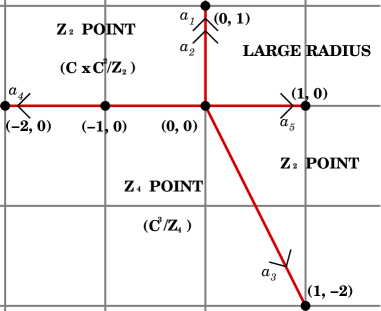
Figure 9: The secondary fan of local $\mathbb{F}_{2}$.

The fan of the toric compactification $\overline{\mathcal{M}^{B,tor}_{2,2}}$ of $\mathcal{M}^{B}_{2,2}$ is simplicial but with marked points: $\overline{\mathcal{M}^{B,tor}_{2,2}}$ is thus a toric orbifold. Its orbifold patches are, as shown in figure 9, a smooth $\mathbb{C}^{2}$ patch containing the large complex structure point, two non-smooth $[\mathbb{C}^{2}/\mathbb{Z}_{2}]$ cones, and finally a $[\mathbb{C}^{2}/\mathbb{Z}_{4}]$ patch parameterized by $(a_{3},a_{4})$. Inspection shows that the latter is a toric orbifold of $\mathbb{C}^{2}$ by the action

$$\begin{array}[]{ccccc}\mathbb{Z}_{4}&\times&\mathbb{C}^{2}&\to&\mathbb{C}^{2}\\ \lambda&&(x,y)&\to&(\lambda x,\lambda^{2}y)\end{array}$$ (6.4)

$(a_{3},a_{4})=(0,0)$ is therefore the only $\mathbb{Z}_{4}$ point in the compactified moduli space as expected. From (6.4) we see that good coordinates around $(a_{3},a_{4})=(0,0)$ are given by

$$a_{3} = \sqrt{d}e$$

$$a_{4} = d^{1/4}$$ (6.5)

Let us then find a complete basis of solutions for the $GKZ$ system around this point. Picard-Fuchs operators are written in this patch as

$$\mathcal{L}_{1} = a_{3}\partial^{2}_{a_{4}}+\frac{1}{2}\theta_{a_{4}}\theta_{a_{3}}$$

$$\mathcal{L}_{2} = \partial^{2}_{a_{3}}-\frac{1}{16}(\theta^{2}_{a_{4}}-4\theta^{2}_{a_{3}})-\frac{1}{4}\theta_{a_{3}}\theta_{a_{4}}$$ (6.6)

and the branch points (5.17) here read

$$\pm c_{1} = \pm\frac{1}{2}\sqrt{a_{4}^{2}-4a_{3}-8}$$

$$\pm c_{2} = \pm\frac{1}{2}\sqrt{a_{4}^{2}-4a_{3}+8}$$ (6.7)

while the period integrals (5.18),(5.19) and (4.17) become

$$\partial_{a_{4}}\Pi_{A} = \frac{K\left(\frac{a_{4}^{2}-4a_{3}-8}{a_{4}^{2}-4a_{3}+8}\right)}{\sqrt{a_{4}^{2}-4a_{3}+8}}-\frac{K\left(\frac{a_{4}^{2}-4a_{3}+8}{a_{4}^{2}-4a_{3}-8}\right)}{\sqrt{a_{4}^{2}-4a_{3}-8}}$$

$$\partial_{a_{4}}\Pi_{B} = 2\frac{K\left(\frac{a_{4}^{2}-4a_{3}-8}{a_{4}^{2}-4a_{3}+8}\right)}{\sqrt{a_{4}^{2}-4a_{3}+8}}$$

$$\Pi_{0_{\pm}} = \log\left(\frac{a_{3}}{2}\pm\frac{\sqrt{a_{3}^{2}-4}}{2}\right)$$ (6.8)

We want to find solutions of the $PF$ system (6.1) with prescribed monodromy around $(d,e)=(0,0)$, in order to match them with the conjugacy classes of $\mathbb{Z}_{4}$. Defining

$$s_{1/4} = \left[\frac{(8-8i)\pi^{1/2}}{\Gamma\left(\frac{1}{4}\right)^{2}}\right]\left(\frac{\Pi_{B}}{2}-\frac{\Pi_{A}}{1-i}\right)$$ (6.9)

$$s_{3/4} = \left[\frac{(4+4i)\Gamma\left(\frac{1}{4}\right)^{2}}{\pi^{3/2}}\right]\left(\frac{\Pi_{B}}{2}+\frac{\Pi_{A}}{1+i}\right)$$ (6.10)

$$s_{1/2} = -2i\Pi_{0_{-}}+\pi$$ (6.11)

we then have

$$s_{1/4}(d,e) = d^{1/4}\left[1+\left(\frac{e^{2}}{32}-\frac{e}{192}+\frac{1}{2560}\right)d-\frac{25e^{3}}{18432}d^{2}+\dots\right]$$ (6.12)

$$s_{1/2}(d,e) = d^{1/2}\Bigg{[}e+\frac{e^{3}d}{24}+\frac{3e^{5}d^{2}}{640}+\frac{5e^{7}d^{3}}{7168}+\dots\Bigg{]}$$ (6.13)

$$s_{3/4}(d,e) = d^{3/4}\left[\left(e-\frac{1}{12}\right)+\left(\frac{3e^{3}}{32}-\frac{3e^{2}}{128}+\frac{9e}{2560}-\frac{3}{14336}\right)d+\dots\right]$$ (6.14)

The normalization of the mirror map has been fixed by imposing the correct asymptotics $s_{1/4}\sim a_{4}$, $s_{1/2}\sim a_{3}$ as to reproduce the generators of the classical orbifold cohomology. These are given by $a_{4}$ and $a_{3}$ respectively for the weight $1/4$ and $1/2$ twisted sectors. Concerning the solution $s_{3/4}$, this is identified with the derivative of the generating function $\mathcal{F}_{orb}$ in (6.1) with respect to $s_{1/4}$; in fact, the orbifold cohomology pairing modifies this relation by a factor of $4$, i.e. $s_{3/4}=4\partial_{s_{1/4}}\mathcal{F}_{orb}$. Taking all this into account, inversion of (6.12) and (6.13) gives the following expression for the prepotential

$$4\frac{\partial\mathcal{F}_{orb}}{\partial s_{1/4}}(s_{1/2},s_{1/4}) = \left(s_{1/2}+\frac{s_{1/2}^{3}}{48}+\frac{s_{1/2}^{5}}{960}+\frac{29s_{1/2}^{7}}{430080}+\frac{457s_{1/2}^{9}}{92897280}+O\left(s_{1/2}^{11}\right)\right)s_{1/4}$$ (6.15)

$$+ \left(-\frac{1}{12}-\frac{s_{1/2}^{2}}{96}-\frac{11s_{1/2}^{4}}{9216}-\frac{49s_{1/2}^{6}}{368640}-\frac{601s_{1/2}^{8}}{41287680}+O\left(s_{1/2}^{10}\right)\right)s_{1/4}^{3}$$

$$+ \left(\frac{7s_{1/2}}{3840}+\frac{s_{1/2}^{3}}{1920}+\frac{47s_{1/2}^{5}}{460800}+\frac{6971s_{1/2}^{7}}{412876800}+O\left(s_{1/2}^{9}\right)\right)s_{1/4}^{5}$$

$$+ \dots$$

As a check, the prepotential thus obtained is invariant under monodromy. The first few orbifold GW invariants are listed in table 2. Our predictions exactly match the results obtained in [51] after the methods of [52].

	$m$	2	4	6	8	10
$n$
0		0	$-\frac{1}{8}$	0	$-\frac{9}{64}$	0
1		$\frac{1}{4}$	0	$\frac{7}{128}$	0	$\frac{1083}{1024}$
2		0	$-\frac{1}{32}$	0	$-\frac{143}{512}$	0
3		$\frac{1}{32}$	0	$\frac{3}{32}$	0	$\frac{85383}{16384}$
4		0	$-\frac{11}{256}$	0	$-\frac{159}{128}$	0
5		$\frac{1}{32}$	0	$\frac{47}{128}$	0	$\frac{360819}{8192}$
6		0	$-\frac{147}{1024}$	0	$-\frac{157221}{16384}$	0
7		$\frac{87}{1024}$	0	$\frac{20913}{8192}$	0	$\frac{73893099}{131072}$
8		0	$-\frac{1803}{2048}$	0	$-\frac{3719949}{32768}$	0
9		$\frac{457}{1024}$	0	$\frac{1809189}{65536}$	0	$\frac{5312434641}{524288}$
10		0	$-\frac{70271}{8192}$	0	$-\frac{498785781}{262144}$	0
11		$\frac{7859}{2048}$	0	$\frac{56072653}{131072}$	0	$\frac{254697581847}{1048576}$
12		0	$-\frac{15933327}{131072}$	0	$-\frac{11229229227}{262144}$	0
13		$\frac{801987}{16384}$	0	$\frac{2354902131}{262144}$	0	$\frac{31371782305803}{4194304}$

Table 2: Genus zero orbifold Gromov-Witten invariants $N^{orb}_{0,(m,n)}$ of $[\mathbb{C}^{3}/\mathbb{Z}_{4}]$.

6.2 Adding D-branes

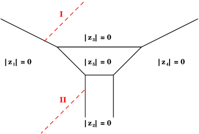
Figure 10: The pq-web of local $\mathbb{F}_{2}$ with lagrangian branes on an upper (I) and lower (II) outer leg.

Following the discussion of section 3.1.1 we might want to turn on an open sector and add Lagrangian branes to the orbifold. The procedure of [34, 35] is in principle valid away from the region of semi-classical geometry and has had a highly non-trivial check for the local $\mathbb{F}_{0}$ case in [8], where open amplitudes have been matched against Wilson lines in the large $N$ dual Chern-Simons theory. First of all, we will consider the setups I and II of figure 10, with a $D$-brane ending respectively on the outer leg $|z_{1}|=|z_{3}|$ and $|z_{1}|=|z_{2}|$. The choice of variables (3.2) we have made for the mirror curve $\Gamma_{2,2}$, in which the $B$-model coordinate mirror to $|z_{2}|$ was gauge-fixed to one, corresponds to phase $II$. This means that $v$ is the variable that goes to one on the brane and $X_{(II)}\equiv u$ is the good open string parameter to be taken as the independent variable in (3.16) [8]. The transition from phase II to phase I is accomplished by the (exponentiated) $SL(2,\mathbb{Z})$ transformation

$$X_{(II)}\equiv u \to \frac{1}{u}\equiv X_{(I)}$$

$$v \to vu^{2}$$ (6.16)

Accordingly, the differential (3.7) has the form

$$d\lambda=\left\{\begin{array}[]{cc}\log{\frac{a_{3}X_{(I)}^{2}+a_{4}X_{(I)}+1+\sqrt{(a_{3}X_{(I)}^{2}+a_{4}X_{(I)}+1)^{2}-4X_{(I)}^{4}}}{2X_{(I)}^{4}}}\frac{dX_{(I)}}{X_{(I)}}&\hbox{phase I}\\ \log{\frac{a_{3}+a_{4}X_{(II)}+X_{(II)}^{2}+\sqrt{(a_{3}+a_{4}X_{(II)}+X_{(II)}^{2})^{2}-4}}{2}}\frac{dX_{(II)}}{X_{(II)}}&\hbox{phase II}\end{array}\right.$$ (6.17)

We now turn to analyze the unframed $A$-model disc amplitude for a brane in phase I. In order to do that we have to compute the instanton corrected open modulus (3.16) and the Abel-Jacobi map (3.14). To determine the former, and more precisely the $r_{i}$ coefficients in (3.16), we use the result of [38], where the authors show that for this outer-leg configuration the large radius open flat variable solving the extended Picard-Fuchs system is given by

$$z^{LR}_{open}=z+\frac{t_{B}}{4}+\frac{t_{F}}{2}+\pi i$$ (6.18)

where $z=\log{X_{(I)}}$. In the ($a_{3}$, $a_{4}$) patch containing the orbifold point this becomes

$$z^{LR}_{open}=z+\pi i+\mathcal{O}(a_{4})+\mathcal{O}(a_{3})$$ (6.19)

Notice that in (6.18), (6.19), both $z^{LR}_{open}$ and $z+\pi i$ solve the extended $PF$ system and can then serve as a flat coordinate: $z^{LR}_{open}$ does the job by construction, and the same is true for $z$ because it is a difference of solutions of the Picard-Fuchs system by (6.18). Following [8], we have that the difference $z^{LR}_{open}-\frac{t_{B}}{4}-\frac{t_{F}}{2}=z+\pi i$ is a global open flat variable and serves as the expansion parameter at the orbifold point. In terms of exponentiated variables, we then have:

$$Z^{orb}_{open}=-X_{(I)}$$ (6.20)

Having the mirror map and using (3.14) or (4) one can then mimic [8] and expand the chain integral, thus obtaining the disc amplitude $\mathcal{F}_{0,1}(a_{3},a_{4},z)$ as a function of the bare variables, or, using (6.12)-(6.13), of the flat variables. Notice that, since $(a_{3},a_{4})$ have non-trivial $\mathbb{Z}_{4}$ transformations, in order to preserve the fact that the curve (5.16) stays invariant we are forced to assign weights $(1/4,1/2)$ to $(u,v)$ respectively, and so according to (6.20) $Z^{orb}_{open}$ has weight $-1/4$. Eventually we get

$$\mathcal{F}_{0,1}(s_{1/4},s_{1/2},Z^{orb}_{open}) = \left(-\frac{s_{1/2}s_{1/4}^{3}}{192}+\frac{s_{1/2}^{2}s_{1/4}}{32}-s_{1/4}\right)Z^{orb}_{open}$$ (6.21)

$$+ \left(\frac{s_{1/2}^{2}s_{1/4}^{2}}{64}-\frac{s_{1/4}^{2}}{4}+s_{1/2}\left(\frac{1}{2}-\frac{s_{1/4}^{4}}{384}\right)\right)(Z^{orb}_{open})^{2}$$

$$+ \left(\frac{7s_{1/2}^{2}s_{1/4}^{3}}{576}-\frac{s_{1/4}^{3}}{9}+\frac{s_{1/2}s_{1/4}}{3}\right)(Z^{orb}_{open})^{3}$$

$$+ \dots$$

which is monodromy invariant. The amplitude (6.21) should correspond to a generating function of open Gromov-Witten invariants of the $\mathbb{C}^{3}/\mathbb{Z}_{4}$ orbifold.
The situation for phase II appears to be more subtle. The resulting topological amplitude computed from the chain integral (3.14) picks up a sign flip under $\mathbb{Z}_{4}$. This is not completely surprising, since it is known that disc amplitudes may have non-trivial monodromy [37], and it might also be seen to be related to the more complicated geometrical structure of the $\mathbb{Z}_{4}$ orbifold with respect to the $\mathbb{Z}_{3}$ case, due to the presence of non-trivial stabilizers for the cyclic group action.

6.3 Modular structure of topological amplitudes

Higher genus amplitudes are associated to the quantization of the symplectic space spanned by the periods of the mirror curve [54]. The corresponding topological wave functional obeys recursion relations (BCOV equations [2]) that allow to compute higher genus amplitudes building on genus zero and one results, up to holomorphic ambiguities. It has been shown in [7] that this algorithm is made simpler and more efficient by exploiting modular properties of the topological amplitudes.

Let us summarize very briefly the results of [7] relevant for our discussion. As recalled in Sect. 3, the choice of $B$-model complex structures can be parametrized in terms of the periods of the three-form $\Omega$ in a chosen symplectic basis $A^{i}\cap B_{j}=\delta^{i}_{j}$ in $H_{3}(\hat{X},\mathbb{Z})$, which define a so-called “real polarization”. Special geometry relations between the periods $x^{i}=\int_{A^{i}}\Omega$ and $p_{j}=\int_{B_{j}}\Omega$ are summarized in terms of a prepotential ${\cal F}_{0}(x^{i})$ which turns out to be the genus zero free-energy of the topological string. The “phase space” $(x^{i},p_{j})$ can be endowed with a natural symplectic structure with symplectic form $dx^{i}\wedge dp_{i}$. The higher genus amplitudes ${\cal F}_{g}$ are associated to the quantization of this space, with the string coupling $g_{s}^{2}$ playing the rôle of $\hbar$. More precisely, the full topological string partition function $Z(x^{i})\sim\exp{\sum_{g}g_{s}^{2g-2}F_{g}(x^{i})}$ is interpreted as a wave function [54]. The periods $(x^{i},p_{j})$ generically undergo an $Sp(2p-2,\mathbb{Z})$ transformation under a change of symplectic basis of the mirror curve. Correspondingly, the $B$-model topological amplitudes ${\cal F}_{g}$ have definite transformation properties that can be derived by implementing the canonical transformation at the quantum level on the topological wave function. The crucial observation of [7] is that there is a finite index subgroup $\Gamma\subset Sp(2p-2,\mathbb{Z})$ which is a symmetry of the theory. $\Gamma$ is precisely the group generated by the monodromies of the periods, which must leave invariant the topological wave-function. This symmetry constrains the topological amplitudes; in particular in the real polarization the ${\cal F}_{g}$ can be shown to be quasi-modular forms of $\Gamma$ [7], namely they transform with a shift. For example for the case of elliptic mirror curves, i.e. local surfaces, this amounts to say that the wave-function is a finite power series in the second Eisenstein series.

We recall that one could also have chosen to parameterize the $B$-model moduli space with the Hodge decomposition of $H^{3}(\hat{X},\mathbb{Z})$ in terms of a fixed background complex structure. The topological wave function in this holomorphic polarization can be shown [54] to obey the BCOV holomorphic anomaly equations. The topological amplitudes $\hat{\cal F}_{g}$ in this case turn out to be proper modular forms of weight zero under $\Gamma$, namely invariant under $\Gamma$, but they are non-holomorphic. For elliptic mirror curves, they can be written in terms of a polynomial in a canonical, non-holomorphic extension of the second Eisenstein series

$$E_{2}(\tau)\to\hat{E_{2}}(\tau,\bar{\tau}):=E_{2}(\tau)-\frac{3}{\pi}\frac{1}{\Im m\tau}$$ (6.22)

with coefficients in the ring of holomorphic modular forms of $\Gamma$. Thus one can pass from the real to the holomorphic polarization just by the above shift of variables.

The advantage of the approach proposed in [7] is twofold. On one side it simplifies the solution of BCOV equations by restricting the functional dependence of the $\hat{\cal F}_{g}$ to the ring of $\Gamma$ modular forms. On the other it allows to relate the topological amplitudes in different patches of the $B$-model moduli space allowing in this way to extract enumerative invariants e.g. at the orbifold point.

As we will show in the following, our method is perfectly tailored to display the modular symmetry of the topological wave-function. In fact, the relation with the Seiberg-Witten curves greatly simplifies the analysis of the modular properties of higher genus amplitudes. Moreover, since we obtain explicit expressions for the periods of the mirror curve in terms of the branch points, it is enough to write the latter in terms of modular forms to make manifest the modular properties of genus zero and one topological amplitudes, thus providing the building blocks for the solution of BCOV equations. About the latter we point out however that there is a caveat: for the geometries under our study in addition to the modular dependence there is also a dependence on an extra parameter (independent of $\tau$), as in the discussion of [7] about the similar case of local $\mathbb{F}_{0}$. This makes the solution of the BCOV equations at higher genus more involved computationally, since one has to fix a functional dependence on an extra datum. We choose to handle this problem with the approach developed in [58, 8] in which the holomorphic ${\cal F}_{g}$ are defined via recurrence relations inspired by matrix-model techniques. This will allow us to display the general modular structure of the free energies in the local $\mathbb{F}_{2}$ case, in a way in which both the dependence on the modular variable and that on the extra parameter are completely fixed.

In this section we first find the relevant change of basis from large radius to the orbifold point and then identify the ring of modular functions relevant for the local $\mathbb{F}_{2}$ case. These results provide the necessary tools to discuss higher genus invariants, which will be the subject of the next section.

6.3.1 The change of basis from large radius

We already saw in the last section that the mirror map at the orbifold point is obtained by choosing solutions of the $GKZ$ system which diagonalize the monodromy of the periods. This implies that the solutions at large radius ($1,t_{B},t_{F},\partial_{F}\mathcal{F}$) are related to those at the orbifold point ($1,s_{1/4},s_{1/2},s_{3/4}$) by a linear transformation, which, for the subsector relating ($t_{F}$, $\partial_{F}\mathcal{F}$) and ($s_{1/2},s_{3/4}$) might be regarded as an (unnormalized) automorphism in $H_{1}(\Gamma_{2,2},\mathbb{Z})$. In [7] it was showed that under a symplectic change of basis

$$\vec{\Pi}\to S\vec{\Pi}=\left(\begin{array}[]{cc}A&B\\ C&D\end{array}\right)\vec{\Pi},\qquad S\in Sp(2p-2,\mathbb{Z})$$ (6.23)

the genus-$g$ amplitudes $\mathcal{F}_{g}$ are subject to a transformation which can be derived by implementing the canonical transformation associated to (6.23) in the path integral defining the topological wave function. From saddle point expansion one then gets

$${\tilde{\cal F}}_{g}={\cal F}_{g}+\Gamma_{g}(\Delta,{\cal F}_{r<g}))$$ (6.24)

where $\Gamma_{g}$ is determined by the Feynman rules in terms of lower genus vertices $\partial^{n}{\cal F}_{r<g}$ and the propagator $\Delta$ given by

$$\Delta\simeq\frac{1}{\tau+C^{-1}D}$$ (6.25)

up to normalization factors. In (6.25) $\tau$ is the period matrix of $\overline{\Gamma}_{2,2}$. This means, for instance, that knowledge of $\mathcal{F}_{g}$ in the large radius region allows one to compute genus-$g$ free energies in the full moduli space, provided that we know how the periods are transformed when going from one region to another. This was successfully exploited in [7] to predict higher genus orbifold Gromov-Witten invariants for the $[\mathbb{C}^{3}/\mathbb{Z}_{3}]$ orbifold from the ones of the large radius $K_{\mathbb{P}^{2}}$ geometry.
We underline that our method of solving the extended GKZ system in the full moduli space has the advantage to make much easier the study of the analytic continuation properties and the consequent computation of the linear change of basis (6.23). Indeed, instead of performing standard (but cumbersome) multiple Mellin-Barnes transforms, we can easily read off what $S$ and $\Delta$ are in our case from formulae (A.2-A.3) and (6.1). Let us define

$$\vec{\Pi}_{LR}=\left(\begin{array}[]{c}1\\ t_{B}\\ t_{F}\\ \partial_{F}\mathcal{F}\end{array}\right)\qquad\vec{\Pi}_{orb}=\left(\begin{array}[]{c}1\\ s_{1/2}\\ s_{1/4}\\ s_{3/4}\end{array}\right)$$ (6.26)

We can now simply compute the change of basis between the large radius and the orbifold point by using the Euler integral representation (A.2) (see also (6.9-6.11)). We can relate $\Pi_{orb}=\tilde{S}\Pi_{LR}$ through

$$\tilde{S}=\left(\begin{array}[]{cc|cc}1&0&0&0\\ \pi&-i&0&0\\ \hline\cr\alpha&\beta&\lx@intercol\hfil\hbox{\multirowsetup{\it S}}\hfil\lx@intercol\\ \gamma&\delta&\\ \end{array}\right)$$ (6.27)

where

$$S=\left(\begin{array}[]{cc}\frac{2\pi^{3/2}}{\Gamma\left(\frac{1}{4}\right)^{2}}&\frac{(1-i)\sqrt{\pi}}{\Gamma\left(\frac{1}{4}\right)^{2}}\\ -\frac{\Gamma\left(\frac{1}{4}\right)^{2}}{\sqrt{\pi}}&\frac{\left(\frac{1}{2}+\frac{i}{2}\right)\Gamma\left(\frac{1}{4}\right)^{2}}{\pi^{3/2}}\end{array}\right)$$ (6.28)

6.3.2 Local $\mathbb{F}_{2}$ and $\Gamma(2)$ modular forms

The last formula in the previous section relates the physical periods of the large radius patch to those of the orbifold patch and represents one of the main ingredients to make predictions about orbifold Gromov-Witten invariants at higher genus. This should be already clear at this stage from (6.24), but it can in fact be brought to full power due to the beautiful results of [7]. Let us see how this works in detail for the $p=2$, $q=2$ case we have been considering, and in particular let us figure out what the relevant modular group $\Gamma$ is in this case. In fact, we have already answered this question: as we stressed in Section 3.3, the family of elliptic curves in this case is the same of its field theory limit, the only thing that changes being the symplectic structure defined on the elliptic fibration, i.e., the $SW$ differential. This was already noticed in the strictly related case of local $\mathbb{F}_{0}$ in [7]. In particular we might argue as follows for the present case. By formulae (3.20), (5.17) the $\Gamma_{2,2}$ family can be written as

$$Y^{2}=(\hat{X}^{2}-c_{1}^{2})(\hat{X}^{2}-c_{2}^{2})$$ (6.29)

where we have shifted the $X$ variable in (3.20) by $\hat{X}=X+a_{4}/2$. Through the following $SL(2,\mathbb{C})$ automorphism of the $\hat{X}$-plane

$$\hat{X}=\frac{a\tilde{X}+b}{c\tilde{X}+d}\qquad\tilde{Y}=(c\tilde{X}+d)^{2}Y$$

$$a=\frac{\sqrt{c_{1}c_{2}-c_{2}^{2}}}{\sqrt{4c_{1}+4c_{2}}},\quad b=\frac{c_{2}(3c_{1}+c_{2})}{2\sqrt{c_{2}\left(c_{1}^{2}-c_{2}^{2}\right)}},\quad c=-\frac{\sqrt{\frac{c_{1}^{2}}{c_{2}}-c_{2}}}{2(c_{1}+c_{2})},\quad d=\frac{c_{1}+3c_{2}}{2\sqrt{c_{2}\left(c_{1}^{2}-c_{2}^{2}\right)}}$$ (6.30)

we bring (6.29) to the celebrated Seiberg-Witten $\Gamma(2)$-symmetric form

$$\tilde{Y}^{2}=(\tilde{X}^{2}-1)(\tilde{X}-u)$$ (6.31)

where

$$u=\frac{c_{1}^{2}+6c_{2}c_{1}+c_{2}^{2}}{(c_{1}-c_{2})^{2}}$$ (6.32)

With (6.32) at hand we can re-express the quantities computed in the previous section as $\Gamma(2)$ modular forms, whose ring is generated by the Jacobi theta functions $\theta_{2}(\tau)$, $\theta_{3}(\tau)$, $\theta_{4}(\tau)$, all having modular weight $1/2$. This goes as follows: the Klein invariant $j(\tau)$ of the curve (6.31) is rationally related to $u$ as

$$j(u)=64\frac{(3+u^{2})^{3}}{(u^{2}-1)^{2}}$$ (6.33)

while inversion of (6.32) gives, writing everything for definiteness in the $(a_{3},a_{4})$ patch,

$$a_{4}^{2}-a_{3}=\frac{u+3}{\sqrt{2}\sqrt{u+1}}$$ (6.34)

Combining the two formulae above and using the definition (5.17) of $c_{1}$, $c_{2}$ we can write the latter as $\Gamma(2)$ modular forms as

$$c_{1}(\tau)=2\frac{\theta_{4}^{2}(\tau)}{\theta_{2}^{2}(\tau)}\qquad c_{2}(\tau)=2\frac{\theta_{3}^{2}(\tau)}{\theta_{2}^{2}(\tau)}$$ (6.35)

which, being coordinates on the moduli space, are correctly modular invariant.

Given (6.35) it is then straightforward to write the building blocks of the BCOV recursion in terms of modular forms. According to [2], the recursion relies on knowledge of the Yukawa coupling $C(\tau)$ and the genus one closed amplitude $\hat{\mathcal{F}}_{1}(\tau,\bar{\tau})$; having exact expressions for the genus zero data as functions of the branch points, one can use (6.35) to write down explicitly all the relevant quantities as modular functions.
Let us analyze the large radius Yukawa coupling first. We have

$$C\equiv\frac{\partial^{3}\mathcal{F}}{\partial t_{F}^{3}}=\frac{4}{\pi}\left(\frac{\partial a_{4}}{\partial\tau}\frac{\partial t_{F}}{\partial a_{4}}\right)^{-1}$$

Using (5.18) we have

$$\frac{\partial t_{F}}{\partial a_{4}}=\frac{K\left(1-\frac{c_{2}^{2}}{c_{1}^{2}}\right)}{c_{1}}=\frac{\pi}{4}\theta_{2}^{2}(\tau)$$ (6.36)

while combining (6.35) and (5.17) yields

$$\frac{\partial a_{4}}{\partial\tau}=-\frac{2^{6}}{a_{4}(\tau)}\frac{\eta^{12}(\tau)}{\theta_{2}(\tau)^{8}}$$ (6.37)

where $\eta(\tau)$ is Dedekind’s function and we have used

$$2\eta^{3}(\tau)=\theta_{2}(\tau)\theta_{3}(\tau)\theta_{4}(\tau)$$ (6.38)

besides the modular expression of $a_{4}$ from (5.17)

$$a_{4}(\tau)=2\sqrt{4\frac{\theta_{4}^{4}(\tau)}{\theta_{2}^{4}(\tau)}+a_{3}+2}$$ (6.39)

Putting it all together we arrive at

$$C(\tau)=-\frac{a_{4}(\tau)}{64}\frac{\theta_{2}^{6}(\tau)}{\eta^{12}(\tau)}$$ (6.40)

Let us now address the issue of the genus 1 free energy $\hat{\mathcal{F}}_{1}(\tau,\bar{\tau})$. For $g=1$ the holomorphic anomaly equation of [2] reads in the local case at hand

$$\partial^{2}_{\bar{t}t}\hat{\mathcal{F}}_{1}(t,\bar{t})=\frac{1}{2}C_{\bar{t}}^{tt}C_{ttt}$$ (6.41)

where indices in (6.41) are raised with the Weyl-Petersson metric $G_{\bar{t}t}=2\Im m\tau$. Rewriting everything as a function of $\tau$, $\bar{\tau}$ (6.41) integrates immediately to

$$\hat{\mathcal{F}}_{1}(\tau,\bar{\tau})=-\frac{1}{2}\log{\Im m\tau}-\log{|\psi(\tau)|}$$ (6.42)

where we have denoted by $\psi(\tau)$ the holomorphic ambiguity at genus one. The pole structure of the amplitude fixes it uniquely; we will do it in the next section by computing explicitly its holomorphic limit.

6.4 Higher genus amplitudes

In this section we will examine the higher genus amplitudes for $K_{\mathbb{F}_{2}}$. After discussing the genus one free energy, we will turn to the analysis of the $g>1$ closed amplitudes, treating in detail the case $g=2$, and we will give predictions for orbifold Gromov-Witten invariants of $\mathbb{C}^{3}/\mathbb{Z}_{4}$ for $g=1,2$.

6.4.1 One loop partition function for $Y^{p,q}$ and genus $1$ orbifold GW

Let us address the issue of the genus 1 free energy in slightly larger generality for the full $Y^{p,q}$ class. In this latter case it would be natural to guess that, again, the same structure as in $SU(p)$ Seiberg-Witten theory holds: monodromy invariance requires it to be written in terms of $\Gamma\subset Sp(2p-2,\mathbb{Z})$ modular forms, and this would lead to the appearance of Siegel modular forms with characteristic. However we happen to have already largely answered this question in the language of hypergeometric functions of the branch points $b_{i}$. Indeed, denoting collectively with $\vec{t}$ the set of flat coordinates, the holomorphic $\vec{\bar{t}}$ limit of $\hat{\mathcal{F}}(\vec{t},\vec{\bar{t}})$ is given on general grounds [2] as

$$\mathcal{F}_{1}(\vec{t})=-\frac{1}{2}\log\mathcal{\det{J}}-\frac{1}{12}\log{\Delta}$$ (6.43)

where $\mathcal{J}$ is the Jacobian matrix of the $A$-periods (in the appropriate polarization) with respect to the bare variables and $\Delta$ is a rational function of the branch points, with zeroes at the discriminant locus of the curve. But it turns out that the awkward Jacobian $\mathcal{J}$ in (6.43) is precisely the main object for which we have found a closed form expression in (1)! This is definitely an advantage with respect to finding a hyperelliptic generalization of the modular symmetry of local surfaces, and in the elliptic case it compendiates nicely the modular expression obtained in the previous section. In the following we will therefore use (6.43) in the local $\mathbb{F}_{2}$ case to obtain a closed expression for $\mathcal{F}_{1}$ in homogeneous (bare) coordinates, and then exploit (6.24) to compute genus 1 orbifold GW invariants of $\mathbb{C}^{3}/\mathbb{Z}_{4}$.

From the considerations above we have at large radius

$$\mathcal{F}_{1}^{LR}(t_{F},t_{B})=-\frac{1}{2}\log\left(\frac{\partial t_{F}}{\partial a_{4}}\right)+\log{\left[c_{1}^{a}c_{2}^{b}(c_{1}-c_{2})^{c}(c_{1}+c_{2})^{d}\right]}$$ (6.44)

where the exponents of the second term are fixed by the topological vertex computation as $a=-1/6$, $b=-1/6$, $c=-1/12$, $d=-1/12$. Then, from (5.17) and (5.18)

$$\mathcal{F}_{1}^{LR}(Q_{F},Q_{B})=-\frac{1}{2}\frac{K\left(1-\frac{c_{2}^{2}}{c_{1}^{2}}\right)}{c_{1}}-\frac{1}{6}\log{c_{1}c_{2}}-\frac{1}{12}\log{\left(c_{1}^{2}-c_{2}^{2}\right)}$$ (6.45)

and plugging in the mirror map (5.22) we can straightforwardly compute

$$\mathcal{F}_{1}^{LR}(Q_{F},Q_{B}) = \left(-\frac{\log(Q_{B})}{24}-\frac{\log(Q_{F})}{12}\right)-\frac{Q_{F}}{6}-\frac{Q_{F}^{2}}{12}-\frac{Q_{F}^{3}}{18}-\frac{Q_{F}^{4}}{24}+$$

$$+ \left(-\frac{Q_{F}}{6}-\frac{Q_{F}^{2}}{3}-\frac{Q_{F}^{3}}{2}\right)Q_{B}+\left(-\frac{Q_{F}^{2}}{12}-\frac{Q_{F}^{3}}{2}+\frac{37Q_{F}^{4}}{6}\right)Q_{B}^{2}+\dots$$

which is the correct form predicted by the topological vertex computation [5]. In order to verify explicitly the assertions of the previous section, we can also use the modular expression of $c_{1}$, $c_{2}$ and $\partial_{a_{4}}t_{F}$ to obtain the holomorphic limit of (6.42) in quasi-modular form. We indeed get

$$\mathcal{F}_{1}^{LR}(\tau)=-\frac{1}{2}\log{\eta(\tau)}$$ (6.47)

Plugging in the expression for the modular parameter $q=e^{2\pi i\tau}$ in exponentiated flat coordinates which can be computed from (5.22), (6.33) and (6.34)

$$q(Q_{B},Q_{F})=Q_{B}Q_{F}^{2}+\left(4Q_{B}^{2}+4Q_{B}\right)Q_{F}^{3}+\left(10Q_{B}^{3}+48Q_{B}^{2}+10Q_{B}\right)Q_{F}^{4}+O\left(Q_{F}^{5}\right)$$ (6.48)

we recover precisely (6.4.1).

	$m$	0	2	4	6	8	10
$n$
0			0	$\frac{1}{128}$	0	$\frac{441}{4096}$	0
1		0	-$\frac{1}{192}$	0	-$\frac{31}{1024}$	0	-$\frac{71291}{32768}$
2		$\frac{1}{96}$	0	$\frac{35}{3072}$	0	$\frac{235}{512}$	0
3		0	-$\frac{5}{768}$	0	-$\frac{485}{4096}$	0	-$\frac{2335165}{131072}$
4		$\frac{7}{768}$	0	$\frac{485}{12288}$	0	$\frac{458295}{131072}$	0
5		0	-$\frac{39}{2048}$	0	-$\frac{40603}{49152}$	0	-$\frac{58775443}{262144}$
6		$\frac{31}{1536}$	0	$\frac{2025}{8192}$	0	$\frac{10768885}{262144}$	0
7		0	-$\frac{2555}{24576}$	0	-$\frac{293685}{32768}$	0	-$\frac{522517275}{131072}$
8		$\frac{2219}{24576}$	0	$\frac{240085}{98304}$	0	$\frac{1437926315}{2097152}$	0
9		0	-$\frac{22523}{24576}$	0	-$\frac{73017327}{524288}$	0	-$\frac{397762755193}{4194304}$
10		$\frac{16741}{24576}$	0	$\frac{54986255}{1572864}$	0	$\frac{32280203275}{2097152}$	0
11		0	-$\frac{389975}{32768}$	0	-$\frac{18440181205}{6291456}$	0	-$\frac{12177409993695}{4194304}$
12		$\frac{1530037}{196608}$	0	$\frac{1434341595}{2097152}$	0	$\frac{7495469356455}{16777216}$	0

Table 3: Genus one orbifold Gromov-Witten invariants $N^{orb}_{1,(m,n)}$ of $[\mathbb{C}^{3}/\mathbb{Z}_{4}]$

Knowing $\mathcal{F}_{1}$ for local $\mathbb{F}_{2}$ we can straightforwardly obtain a prediction for genus one orbifold Gromov-Witten invariants of $\mathbb{C}^{3}/\mathbb{Z}_{4}$; to relate (6.4.1) to the expansion of the $g=1$ topological partition function at the orbifold point we just need to specialize the Feynman expansion (6.24) to the case at hand. The one loop term is given as

$$\Gamma_{1}=\frac{1}{2}\log{\frac{4}{\mathcal{\tau}+C^{-1}D}}$$ (6.49)

where the factor of $4$ comes again from the orbifold cohomology pairing. The genus one orbifold free energy will be then given as

$$\mathcal{F}^{orb}_{1}=\mathcal{F}^{LR}_{1}+\Gamma_{1}$$ (6.50)

where $\tau$ can be written as a function of the $a_{i}$ variables using (5.18), (5.19) or directly as an expansion in orbifold flat coordinates using (6.28). We can now rewrite everything in terms of $s_{1/2}$, $s_{1/4}$ by plugging the orbifold mirror map (6.13) into the expression (6.44) of $\mathcal{F}_{1}^{LR}$, yielding

$$\mathcal{F}_{1}^{orb}(s_{1/4},s_{1/2}) = \sum_{n,m}\frac{N^{orb}_{1,(m,n)}}{n!m!}s_{1/4}^{m}s_{1/2}^{n}$$

$$= -\frac{s_{14}^{2}s_{12}}{384}+\frac{s_{12}^{2}}{192}-\frac{5s_{14}^{2}s_{12}^{3}}{9216}+\frac{7s_{12}^{4}}{18432}-\frac{13s_{14}^{2}s_{12}^{5}}{163840}+\frac{31s_{12}^{6}}{1105920}+\dots$$

The same result would be obtained by using a modified expression for the Jacobian in (6.43) adapted to the orbifold patch, i.e. by replacing $\partial_{a_{4}}t_{F}$ in (6.44) with $\partial_{a_{4}}s_{1/4}$, without then considering the extra piece (6.49) from the Feynman expansion. The first few GW invariants are reported in table 3.

6.4.2 Generalities on $g>1$ free energies

Turning now to the case of $g>1$ closed amplitudes, let us first of all recall the main statements put forward in [7, 56] for the computation of higher genus free energies. As mentioned in section 6.3.2, modular symmetry is an amazingly stringent constraint. For 1-parameter models with elliptic mirror curve (like $SU(2)$ Seiberg-Witten theory, or local $\mathbb{P}_{2}$) the authors of [7, 56] claim that solutions of the genus $g$ holomorphic anomaly equations can be written for $g\geq 2$ as

$$\hat{\mathcal{F}}_{g}(\tau,\bar{\tau})=C^{2g-2}(\tau)\sum_{k=1}^{n}\hat{E}^{k}_{2}(\tau,\bar{\tau})c^{(g)}_{k}(\tau)+C^{2g-2}(\tau)c^{(g)}_{0}(\tau)$$ (6.52)

where $\tau$ is the complex modulus of the mirror torus, $C$ is the Yukawa coupling $\partial^{3}_{t}\mathcal{F}_{0}$, $c_{k}^{(g)}(\tau)$ are $\Gamma$-modular forms of weight $6(g-1)-2k$ and the full non-holomorphic dependence of $\hat{\mathcal{F}}_{g}$ is captured by the modular, non-holomorphic extension of the second Eisenstein series (6.22).

Now, there are two ways to compute the expressions in (6.52). The first one consists in a direct study of the BCOV equations: in this context the holomorphic modular coefficients $c_{k}^{(g)}$ for $k>0$ can either be fixed by the Feynman expansion (6.24) in terms of derivatives of lower genus $\mathcal{F}_{g^{\prime}}$, or much more efficiently by exploiting the modular symmetry to perform a direct integration of the holomorphic anomaly equations as in [56].
Within this method, the only real issue is to fix the so-called “holomorphic ambiguity” at $k=0$, i.e. $c^{(g)}_{0}(\tau)$. In the 1-parameter cases analyzed in [7, 56], this is systematically done by plugging into (6.52) an ansatz for $c^{(g)}_{0}(\tau)$ which is then determined from extra boundary data. More in detail, this works as follows: at fixed genus $g$, $c^{(g)}_{0}(\tau)$ is a weight $w=6g-3$ modular form. Now, the ring of weight $w$ holomorphic modular forms $\mathcal{M}_{w}(\Gamma)$ is finitely generated, and the analytic behavior of $\mathcal{F}_{g}(\tau,\bar{\tau})$ at large radius allows to write an ansatz for $c^{(g)}_{0}(\tau)$ with only a finite number of unknown coefficients. At the same time, $c^{(g)}_{0}(\tau)$ is constrained to satisfy the so-called “gap condition” [57]: this imposes a sufficient number of constraints to completely determine (indeed, overdetermine) the conjectured form of the ambiguity as a function of the generators of $\mathcal{M}_{w}(\Gamma)$.
The discussion of section 6.3.2 has shown that the case of local $\mathbb{F}_{2}$ is in many ways similar to the simpler examples of $SU(2)$ Seiberg-Witten theory and local $\mathbb{P}^{2}$. However there is an extra complication, given by the fact that the elliptic modulus $\tau$ is not the only variable in the game: here we actually have an extra bare parameter $a_{3}$, or $z_{B}$, which is independent on $\tau$ and is related to the Kähler volume of the base $\mathbb{P}^{1}$ (see (4.17), (6.1)). That is, we deal here with a two-parameter model, even though with an elliptic mirror curve, and we have to properly take this into account. A first consequence of this fact is that the idea of using the gap condition to fix the holomorphic ambiguity becomes computationally more complicated, since our task is no longer reduced to fix simply a finite set of unknown numerical coefficients of $c^{(g)}_{0}(\tau)$ as generated by a basis of $\mathcal{M}_{w}(\Gamma)$: rather we should fix a finite set of unknown functions of $a_{3}$.

A second possibility is to avail ourselves of the framework proposed in [8] for the computation of topological string amplitudes based on the Eynard-Orantin recursion for matrix models. This is based on a sequence of polydifferentials $W_{h}^{(g)}$ on the mirror curve $\Gamma$, which are recursively computed in terms of residue calculus on $\Gamma$ and out of which it is possible to extract the free energies $\mathcal{F}_{g}$ at any given genus. Let us briefly review here this formalism in order to describe the general structure of higher amplitudes, referring the reader to [8, 58] for further details.
The ingredients needed are the same as for genus zero amplitudes, namely the family of Hori-Vafa mirror curves $H(u,v)=0$ (3.2) with differential $d\lambda$ (3.7). The genus $g$ free energies are then recursively given as

$$\mathcal{F}_{g}={1\over 2-2g}\sum_{b_{i}}\underset{u=b_{i}}{\rm Res~{}}\phi(u)W_{1}^{(g)}(u).$$ (6.53)

where $\phi(u)$ is any antiderivative of the Hori-Vafa differential

$$d\phi(u)=d\lambda(u)=\log{v(u)}\frac{du}{u}$$ (6.54)

and $W_{h}^{(g)}(p_{1},\ldots,p_{h})$ with $g,h\in\mathbb{Z}^{+}$, $h\geq 1$ are an infinite sequence of meromorphic differentials on the curve defined by the Eynard-Orantin recursion

$$W_{1}^{(0)}(p_{1})=0,\qquad W_{2}^{(0)}(p_{1},p_{2})=B(p_{1},p_{2}),$$ (6.55)

$$W_{h+1}^{(g)}(p,p_{1}\ldots,p_{h}) = \sum_{b_{i}}\underset{q=b_{i}}{\rm Res~{}}{dE_{q}(p)\over d\lambda(q)-d\lambda(\bar{q})}\Big{(}W^{(g-1)}_{h+2}(q,\bar{q},p_{1},\ldots,p_{h})$$ (6.56)

$$+ \sum_{l=0}^{g}\sum_{J\subset H}W^{(g-l)}_{|J|+1}(q,p_{J})W^{(l)}_{|H|-|J|+1}(\bar{q},p_{H\backslash J})\Big{)}.$$

In the formulae above, $\bar{q}$ denotes the conjugate point to $q$, $B(p,q)$ is the Bergmann kernel, the one form $dE_{q}(p)$ is given as

$$dE_{q}(p)=\frac{1}{2}\int_{q}^{\bar{q}}B(p,\xi)d\xi$$ (6.57)

and finally, given any subset $J=\{i_{1},\cdots,i_{j}\}$ of $H:=\{1,\cdots,h\}$, we defined $p_{J}=\{p_{i_{1}},\cdots,p_{i_{j}}\}$. We refer the reader to [8, 58] for an exhaustive description of the objects introduced above.

At a computational level, the formalism of [8] is somewhat lengthier than the one of [56] for computing higher genus $\mathcal{F}_{g}$. On the other hand, the recursion of [8] has the great advantage of providing unambiguous results, with the holomorphic ambiguity $c^{(g)}_{0}(\tau)$ automatically fixed. This precisely overcomes the problem raised above. In the next section, we will therefore follow this second path to complete the discussion of section 6.3.2 by displaying explicitly the modular structure of the $\mathcal{F}_{g}$ obtained through (6.53). An explicit computation of the $g=2$ case, as well as predictions at the orbifold point, will be left to section 6.4.4.

6.4.3 $g>1$ and modular forms

Let us specialize the recursion to the case of local $\mathbb{F}_{2}$. The Hori-Vafa differential (4.3) reads, in the $(a_{3},a_{4})$ patch,

$$d\lambda_{2,2}(u)=\log\left(\frac{P_{2}(u)\pm Y(u)}{2}\right)\frac{du}{u}$$ (6.58)

where

$$P_{2}(u)=a_{3}+a_{4}u+u^{2},\qquad Y(u)=\sqrt{P_{2}^{2}(u)-4}$$

and the $\Gamma_{2,2}$ family can be written in the $\mathbb{Z}_{2}$ symmetric form (6.29) as a two-fold branched covering of the compactified $u$-plane

$$Y^{2}=(u-b_{1})(u-b_{2})(u-b_{3})(u-b_{4})=(\hat{u}^{2}-c_{1}^{2})(\hat{u}^{2}-c_{2}^{2})$$ (6.59)

thanks to (5.17) and (6.29) and having defined $\hat{u}=u+a_{4}/2$. We have first of all that

$$d\lambda(u)-d\lambda(\bar{u})=2M(u)Y(u)du$$ (6.60)

where the so-called “moment function” $M(u)$ is given, after using the fact that $\log({P+Y})-\log({P-Y})=2\tanh^{-1}{(Y/P)}$, as

$$M(u)={1\over uY(u)}\tanh^{-1}\biggl{[}{{Y(u)}\over P_{2}(u)}\biggr{]},$$ (6.61)

Moreover, the one form $dE(p,q)$ can be written as [58]

$$dE_{w}(u)={1\over 2}{Y(w)\over Y(u)}\,\left({1\over u-w}-LC(w)\right)\,du$$ (6.62)

where

$$C(w):={1\over 2\pi i}\,\oint_{A}{du\over{Y(u)}}\,{1\over u-w},\qquad L^{-1}:={1\over 2\pi i}\,\oint_{A}{du\over{Y(u)}}$$ (6.63)

We have assumed here that $w$ stays outside the contour $A$; when $w$ lies inside the contour $A$, $C(w)$ in (6.62) should be replaced by its regularized version

$$C^{\rm reg}(w)=C(w)-\frac{1}{Y(w)}$$ (6.64)

Since $\Gamma_{2,2}$ is elliptic, it is possible to find closed form expressions for $C(u)$, $C_{reg}(u)$, $B(u,w)$ and $L$. We have

$$C(u)={2(b_{2}-b_{3})\over\pi(u-b_{3})(u-b_{2}){\sqrt{(b_{1}-b_{3})(b_{2}-b_{4})}}}\biggl{[}\Pi(n_{4},k)+\frac{u-b_{2}}{b_{2}-b_{3}}K(k)\biggr{]}$$ (6.65)

$$C^{\rm reg}(u)={2(b_{3}-b_{2})\over\pi(u-b_{3})(u-b_{2}){\sqrt{(b_{1}-b_{3})(b_{2}-b_{4})}}}\biggl{[}\Pi(n_{1},k)+\frac{u-b_{3}}{b_{3}-b_{2}}K(k)\biggr{]}$$ (6.66)

$$L^{-1}=\frac{2}{\sqrt{(b_{1}-b_{3})(b_{2}-b_{4})}}K\left[\frac{(b_{1}-b_{2})(b_{3}-b_{4})}{(b_{1}-b_{3})(b_{2}-b_{4})}\right]$$ (6.67)

$$B(u,w) = \frac{1}{Y(u)}\left[\frac{Y^{2}(u)}{2Y(w)(u-w)^{2}}+\frac{(Y^{2})^{\prime}(u)}{4Y(w)(w-u)}+\frac{A(u)}{4Y(w)}\right]$$ (6.68)

$$+ \frac{1}{2(u-w)^{2}}$$

where

$$k={(b_{1}-b_{2})(b_{3}-b_{4})\over(b_{1}-b_{3})(b_{2}-b_{4})},\qquad n_{4}={(b_{2}-b_{1})(u-b_{3})\over(b_{3}-b_{1})(u-b_{2})},\qquad n_{1}={(b_{4}-b_{3})(u-b_{2})\over(b_{4}-b_{2})(u-b_{3})},$$ (6.69)

$$A(u)=(u-b_{1})(u-b_{2})+(u-b_{3})(u-b_{4})+(b_{1}-b_{3})(b_{2}-b_{4})\frac{E(k)}{K(k)}$$ (6.70)

and $K(k)$, $E(k)$ and $\Pi(n,k)$ are the complete elliptic integrals of the first, second and third kind respectively.

With these ingredients one can compute the residues as required in (6.56). Given that $dE_{q}(p)/(d\lambda(q)-d\lambda(\bar{q}))$, as a function of $q$, is regular at the branch-points, all residues appearing in (6.56) will be linear combinations of the following kernel differentials

$$\chi_{i}^{(n)}(p) = {\rm Res}_{q=x_{i}}\biggl{(}\frac{dE_{q}(p)}{d\lambda(q)-d\lambda(\bar{q})}{1\over(q-x_{i})^{n}}\biggr{)}$$ (6.71)

$$= {1\over(n-1)!}{1\over{Y(p)}}{d^{n-1}\over dq^{n-1}}\Biggl{[}{1\over 2M(q)}\biggl{(}{1\over p-q}-LC(q)\biggl{)}\Biggr{]}_{q=x_{i}}$$

In (6.71), $C(p)$ should be replaced by $C_{\rm reg}(p)$ when $i=1,2$.

Let us then explicitly display the quasi-modular structure of the free energies $\mathcal{F}_{g}(a_{3},\tau)$. We claim that the holomorphic limit of the $1$-parameter examples (6.52)

$$\mathcal{F}_{g}(\tau)=C^{2g-2}(\tau)\sum_{k=1}^{n}E^{k}_{2}(\tau)c^{(g)}_{k}(\tau)+C^{2g-2}(\tau)c^{(g)}_{0}(\tau)$$

gets replaced here by

$$\mathcal{F}_{g}(a_{3},\tau)=C^{2g-2}(a_{3},\tau)\sum_{k=1}^{n}E^{k}_{2}(\tau)c^{(g)}_{k}(a_{3},\tau)+C^{2g-2}(a_{3},\tau)c^{(g)}_{0}(a_{3},\tau)$$ (6.72)

i.e., as a polynomial in the second Eisenstein series having (algebraic) functions of $a_{3}$ and $\theta_{i}(\tau)$, $i=2,3,4$ as coefficients; moreover, these coefficients are completely determined in closed form from (6.56). Let us show in detail how this happens in general, leaving the concrete example of the $g=2$ case to the next section. Formulae (6.53), (6.56), (6.68) and (6.71) imply that the final answer will be a polynomial in the following five objects

$$M_{i}^{(n)},\qquad\phi^{(n)}_{i},\qquad A^{(n)}_{i},\qquad\left(\frac{1}{Y}\right)_{i}^{(n)},\qquad\mathcal{C}^{(n)}_{i}$$ (6.73)

where, for a function $f(x)$ with meromorphic square $f^{2}(x)$, we denote with $f^{(n)}_{i}$ the $(n+1)$-th coefficient in a Laurent expansion of $f(x)$ around $b_{i}$

$$f(x)=\sum_{n=-N_{i}}^{\infty}\frac{f_{i}^{(n+N_{i})}}{(p-b_{i})^{n/2}}$$ (6.74)

and have defined

$$\mathcal{C}^{(n)}_{i}=\left\{\begin{array}[]{cc}C^{(n)}_{{\rm reg},i}&\mathrm{for}\quad i=1,2\\ C^{(n)}_{i}&\mathrm{for}\quad i=3,4\end{array}\right.$$ (6.75)

Of the five building blocks in (6.73), $M_{i}^{(n)}$ and $\phi^{(n)}_{i}$ are the ones which are computed most elementarily from (6.58), (6.54) and (6.61), the result being in any case an algebraic function of $(a_{3},a_{4})$. When re-expressed in modular form, we can actually say more about them: we have that the $a_{3}$-dependence in $M_{i}^{(n)}(a_{3},\tau)$ and $\phi^{(n)}_{i}(a_{3},\tau)$ is constrained to come only through $a_{4}(a_{3},\tau)$ as written in formula (6.39). Indeed, from (5.17), (6.35) we have that the branch points $b_{i}$ have the form

$$-\frac{a_{4}}{2}\pm c_{1}(\tau),\qquad-\frac{a_{4}}{2}\pm c_{2}(\tau)$$ (6.76)

and therefore depend on $a_{3}$ only through $a_{4}(a_{3},\tau)$. Moreover, since $P_{2}(b_{i})=2$ and the derivatives of $P_{2}(u)$ do not depend explicitly on $a_{3}$, we have that the $a_{3}$ dependence in $\mathcal{F}_{g}$ as obtained from the recursion may only come through $a_{4}(a_{3},\tau)$. Notice moreover that these are the only pieces bringing a dependence on the additional $a_{3}$ variable: all the others do not depend on the form of the differential (6.58), and are functions only of differences of branch points $b_{i}$. This means in particular that they only depend on the variables $c_{1}$ and $c_{2}$ introduced in (5.17) and whose modular expressions we already found in (6.35)! This is immediate to see for $A^{(n)}_{i}$ and $(1/Y)_{i}^{(n)}$ from formulae (6.59) and (6.70). The case of $\mathcal{C}^{(n)}_{i}$ is just slightly more complicated, but it is worth describing in detail for the discussion to come. For $n=1$, we need the first derivative of $\Pi(x,y)$ with respect to $x$:

$$\partial_{x}\Pi(x,y)=\frac{xE(y)+(y-x)K(y)+\left(x^{2}-y\right)\Pi(x,y)}{2(x-1)x(y-x)}$$

The above formula implies that

$$\partial^{(n)}_{x}\Pi(x,y)=A_{n}(x,y)K(y)+B_{n}(x,y)E(y)+C_{n}(x,y)\Pi(x,y)$$ (6.77)

where $A_{n}$, $B_{n}$ and $C_{n}$ are rational functions of $x$ and $y$. From (6.69), to compute $\mathcal{C}^{(n)}_{i}$, we need to evaluate these expressions when $n_{1}$ (resp. $n_{4}$) equals either 0 or $k$. But using

$$\Pi(0,y)=K(y),\qquad\Pi(y,y)=\frac{E(y)}{1-y}$$ (6.78)

we conclude that

$$\mathcal{C}^{(n)}_{i}=R^{(n)}_{1}(c_{1},c_{2})K(k)+R^{(n)}_{2}(c_{1},c_{2})E(k)$$ (6.79)

for two sequences of rational functions $R^{(n)}_{i}$. We now make the following basic observation: by (6.71), $\mathcal{C}^{(n)}_{i}$ always appears multiplied by $L$ in the recursion. By (6.67)

$$L\mathcal{C}^{(n)}_{i}=\tilde{R}^{(n)}_{1}(c_{1},c_{2})+\tilde{R}^{(n)}_{2}(c_{1},c_{2})\frac{E(k)}{K(k)}$$ (6.80)

This last observation allows us to collect all the pieces together and state the following. By (6.56) and (6.53) we have that $\mathcal{F}_{g}(a_{3},\tau)$ is a polynomial in $M_{i}^{(n)}$, $\phi^{(n)}_{i}$, $A^{(n)}_{i}$, $(1/Y)_{i}^{(n)}$, $\mathcal{C}^{(n)}_{i}$, and moreover the whole discussion above as well as formulae (6.70) and (6.80) imply that this takes the form of a polynomial in $W(\tau):=E(k)/K(k)$

$$\mathcal{F}_{g}(a_{3},\tau)=\sum_{k=0}^{n}W^{k}(\tau)h^{(g)}_{k}(a_{3},\tau)$$ (6.81)

with coefficients $h^{(g)}_{k}(a_{3},\tau)$ in the ring of weight zero modular forms of $\Gamma(2)$, parametrically depending on $a_{3}$.
To conclude, we can exploit the fact that [59]

$$E(k)K(k)=\left(\frac{\pi}{2}\right)^{2}\frac{4E_{2}(2\tau)-E_{2}(\tau)}{3}$$ (6.82)

and that from (6.35) and (6.36)

$$K(k)=\frac{\pi}{2}\theta_{3}(\tau)\theta_{4}(\tau)$$ (6.83)

where we have used the fact that in our case

$$K(k)=\sqrt{\frac{c_{2}}{c_{1}}}K\left(1-\frac{c_{2}^{2}}{c_{1}^{2}}\right)$$

as the reader can easily check. Moreover, the second Eisenstein series satisfies the duplication formula

$$E_{2}(2\tau)=\frac{E_{2}(\tau)}{2}+\frac{\theta_{4}^{4}(\tau)+\theta_{3}^{4}(\tau)}{4}$$ (6.84)

Therefore,

$$W(\tau)=\frac{1}{3\theta_{4}^{2}(\tau)\theta_{3}^{2}(\tau)}\left(E_{2}(\tau)+\theta_{3}^{4}(\tau)+\theta_{4}^{4}(\tau)\right)$$ (6.85)

This proves (6.72).

6.4.4 The $g=2$ case in detail

Let us complete the discussion of this section by presenting the explicit formulae for the genus 2 case. By (6.53) and (6.56), we need the complete expression of $W_{2}^{(0)}$, $W_{3}^{(0)}$, $W_{1}^{(1)}$, $W_{2}^{(1)}$ and $W_{1}^{(2)}$. The first three were computed in [8] and are given by

$$W_{2}^{(0)}(p_{1},p_{2}) = B(p_{1},p_{2})$$

$$W_{3}^{(0)}(p_{1},p_{2},p_{3}) = {1\over 2}\sum_{i=1}^{4}M^{2}(b_{i})(Y^{2})^{\prime}(b_{i})\chi^{(1)}_{i}(p_{1})\chi^{(1)}_{i}(p_{2})\chi^{(1)}_{i}(p_{3}),$$ (6.86)

$$W_{1}^{(1)}(p) = {1\over 16}\sum_{i=1}^{4}\chi^{(2)}_{i}(p)+{1\over 8}\sum_{i=1}^{4}\biggl{(}\frac{2A(b_{i})}{(Y^{2})^{\prime}(b_{i})}-\sum_{j\not=i}{1\over b_{i}-b_{j}}\biggr{)}\chi_{i}^{(1)}(p),$$

$W_{2}^{(1)}$ is then given from (6.56) as

$$W_{2}^{(1)}(p,p_{1})=\sum_{b_{i}}\underset{q=b_{i}}{\rm Res~{}}{dE_{q}(p)\over d\lambda(q)-d\lambda(\bar{q})}\Big{(}W^{(0)}_{3}(q,\bar{q},p_{1})+2W^{(1)}_{1}(q)W^{(0)}_{2}(\bar{q},p_{1})\Big{)}$$ (6.87)

A very lengthy, but straightforward computation leads us to

$$W_{2}^{(1)}(p,q)=-\frac{1}{8}\sum_{i=1}^{4}\left[A_{i}(q)\chi_{i}^{(3)}(p)+B_{i}(q)\chi_{i}^{(2)}(p)+C_{i}(q)\chi_{i}^{(1)}(p)+\sum_{j\neq i}D_{ij}(q)\chi_{i}^{(1)}(p)\right]$$ (6.88)

For the sake of notational brevity, we spare to the reader the very long expressions of the rational functions $A_{i}(q)$, $B_{i}(q)$, $C_{i}(q)$ and $D_{ij}(q)$. They involve $M_{i}^{(n)}$, $A^{(n)}_{i}$, $(1/Y)_{i}^{(n)}$ and $\mathcal{C}^{(n)}_{i}$ up to the third order in a Taylor-Laurent expansion around the branch points.

The next step is given by

$$W_{1}^{(2)}(p)=\sum_{b_{i}}\underset{q=b_{i}}{\rm Res~{}}{dE_{q}(p)\over d\lambda(q)-d\lambda(\bar{q})}\Big{(}W^{(1)}_{2}(q,\bar{q})+W^{(1)}_{1}(q)W^{(1)}_{1}(\bar{q})\Big{)}$$ (6.89)

The pole structure of $A_{i}(q)$, $B_{i}(q)$, $C_{i}(q)$ and $D_{ij}(q)$ dictates for $W_{1}^{(2)}(p)$ the following linear expression in terms of kernel differentials

$$W_{1}^{(2)}(p)=\sum_{n=1}^{5}\sum_{i=1}^{4}E^{(n)}_{i}\chi_{i}^{(n)}(p)$$ (6.90)

for some (very complicated) coefficients $E_{i}^{(n)}$. The recursion is finalized for $g=2$ by (6.53)

$$\mathcal{F}_{2}=-{1\over 2}\sum_{b_{i}}\underset{p=b_{i}}{\rm Res~{}}\phi(p)W_{1}^{(2)}(p)$$ (6.91)

It is useful to collect together terms involving the same powers of $W(\tau)$. Taking the residues in (6.91) yields

$$\sum_{n=0}^{3}h^{(2)}_{n}(a_{3},\tau)W^{n}(\tau)$$ (6.92)

where

$$h^{(2)}_{3}(a_{3},\tau) = \frac{5a_{4}^{2}(a_{3},\tau)\theta_{2}^{4}(\tau)}{24576\theta_{3}^{2}(\tau)\theta_{4}^{2}(\tau)}$$

$$h^{(2)}_{2}(a_{3},\tau) = \frac{1}{1024}-\frac{a_{4}(a_{3},\tau)^{2}}{49152\theta_{3}(\tau)^{6}\theta_{4}(\tau)^{4}}\Bigg{[}\theta_{2}(\tau)^{4}(15\theta_{4}(\tau)^{6}+16\theta_{3}(\tau)^{2}\theta_{4}(\tau)^{4}$$

$$+ \theta_{2}(\tau)^{4}\left(8\theta_{3}(\tau)^{2}+15\theta_{4}(\tau)^{2}\right))\Bigg{]}$$

$$h^{(2)}_{1}(a_{3},\tau) = -\frac{\left(\theta_{2}(\tau)^{4}+2\theta_{4}(\tau)^{4}+3\theta_{3}(\tau)^{2}\theta_{4}(\tau)^{2}\right)}{3072\theta_{4}(\tau)^{2}\theta_{3}(\tau)^{2}}+\frac{a_{4}^{2}(a_{3},\tau)}{294192}\Bigg{[}\frac{13\theta_{2}(\tau)^{12}}{\theta_{3}(\tau)^{6}\theta_{4}(\tau)^{6}}$$

$$+ \frac{91\theta_{2}(\tau)^{8}}{\theta_{3}(\tau)^{6}\theta_{4}(\tau)^{2}}+\frac{48\theta_{2}(\tau)^{8}}{\theta_{3}(\tau)^{4}\theta_{4}(\tau)^{4}}+\frac{91\theta_{4}(\tau)^{2}\theta_{2}(\tau)^{4}}{\theta_{3}(\tau)^{6}}+\frac{96\theta_{2}(\tau)^{4}}{\theta_{3}(\tau)^{4}}\Bigg{]}$$

$$h^{(2)}_{0}(a_{3},\tau) = \frac{1}{61440}\left(\frac{1}{a_{3}+2}-\frac{1}{a_{3}-2}\right)+\frac{\theta_{2}(\tau)^{8}-5\theta_{3}(\tau)^{2}\theta_{2}(\tau)^{4}+10\theta_{3}(\tau)^{6}}{30720\theta_{3}(\tau)^{4}\theta_{4}(\tau)^{4}}$$ (6.93)

$$+ \frac{a_{4}^{2}(a_{3},\tau)\theta_{2}(\tau)^{4}}{2949120}\Bigg{[}12\left(\frac{\theta_{2}(\tau)^{4}}{\theta_{3}(\tau)^{8}}-\frac{\theta_{2}(\tau)^{4}}{\theta_{4}(\tau)^{8}}\right)-\frac{65\theta_{4}(\tau)^{2}}{\theta_{3}(\tau)^{6}}-\frac{175}{\theta_{3}(\tau)^{2}\theta_{4}(\tau)^{2}}$$

$$- \frac{311}{2\theta_{3}(\tau)^{4}}-\frac{311}{2\theta_{4}(\tau)^{4}}-\frac{65\theta_{3}(\tau)^{2}}{\theta_{4}(\tau)^{6}}\Bigg{]}+\frac{17}{46080}$$

Plugging in the expression (6.48) of the modular parameter $q$ in exponentiated flat coordinates reproduces as expected the topological vertex expansion at large radius

$$\mathcal{F}_{2}^{LR}(Q_{B},Q_{F}) = \left(-\frac{1}{120}-\frac{Q_{B}}{120}\right)Q_{F}+\left(-\frac{1}{60}-\frac{Q_{B}}{60}-\frac{Q_{B}^{2}}{60}\right)Q_{F}^{2}$$ (6.94)

$$+ \left(-\frac{1}{40}-\frac{Q_{B}}{40}-\frac{Q_{B}^{2}}{40}-\frac{Q_{B}^{3}}{40}\right)Q_{F}^{3}+\left(-\frac{1}{30}-\frac{Q_{B}}{30}-\frac{Q_{B}^{2}}{6}-\frac{Q_{B}^{3}}{30}\right)Q_{F}^{4}$$

$$+ \left(-\frac{1}{24}-\frac{Q_{B}}{24}-\frac{299Q_{B}^{2}}{24}-\frac{299Q_{B}^{3}}{24}\right)Q_{F}^{5}++O\left(Q_{F}^{6}\right)$$

Finally, we can use (6.92) to make predictions for genus 2 orbifold Gromov-Witten invariants of $\mathbb{C}^{3}/\mathbb{Z}_{4}$ by using the Feynman expansion method of [2, 7] as we did for the genus 1 free energy; the same result would be obtained by analytically continuing the holomorphic ambiguity $h^{(2)}_{0}(a_{3},\tau)$ and taking the holomorphic limit of the physical amplitude directly at the orbifold point (see [60] for a detailed description of this method). The results are shown in table 4.

	$m$	0	2	4	6	8	10
$n$
0		$-\frac{1}{960}$	0	$-\frac{61}{30720}$	0	$-\frac{9023}{81920}$	0
1		0	$\frac{41}{46080}$	0	$\frac{6061}{245760}$	0	$\frac{36213661}{7864320}$
2		$-\frac{7}{7680}$	0	$-\frac{647}{92160}$	0	$-\frac{1066027}{1310720}$	0
3		0	$\frac{257}{92160}$	0	$\frac{168049}{983040}$	0	$\frac{887800477}{15728640}$
4		$-\frac{11}{5120}$	0	$-\frac{65819}{1474560}$	0	$-\frac{18530321}{1966080}$	0
5		0	$\frac{23227}{1474560}$	0	$\frac{43685551}{23592960}$	0	$\frac{62155559923}{62914560}$
6		$-\frac{2479}{245760}$	0	$-\frac{437953}{983040}$	0	$-\frac{9817250341}{62914560}$	0
7		0	$\frac{418609}{2949120}$	0	$\frac{452348269}{15728640}$	0	$\frac{5851085490887}{251658240}$
8		$-\frac{19343}{245760}$	0	$-\frac{303139073}{47185920}$	0	$-\frac{438364727389}{125829120}$	0
9		0	$\frac{1380551}{737280}$	0	$\frac{25384681949}{41943040}$	0	$\frac{355405937648809}{503316480}$
10		$-\frac{604199}{655360}$	0	$-\frac{2982122587}{23592960}$	0	$-\frac{16896151842371}{167772160}$	0
11		0	$\frac{200852963}{5898240}$	0	$\frac{25012290702059}{1509949440}$	0	$\frac{54049855936801961}{2013265920}$
12		$-\frac{59566853}{3932160}$	0	$-\frac{818897894611}{251658240}$	0	$-\frac{1840152188554961}{503316480}$	0

Table 4: Genus two orbifold Gromov-Witten invariants $N^{orb}_{2,(m,n)}$ of $[\mathbb{C}^{3}/\mathbb{Z}_{4}]$

7 Conclusions and outlook

In this paper we have proposed an approach to the study of $A$-model topological amplitudes which yields exact results in $\alpha^{\prime}$ and as such applies to the full moduli space, including orbifold and conifold divisors, of closed and open strings on a large class of toric Calabi-Yau threefolds. One of the main virtues of this approach is that it provides us with a closed expression for the (derivatives of the) periods of the mirror curve, considerably simplifying the study of their analytic continuation in the various patches and of the modular properties of the Gromov-Witten generating functional. The local geometries that we have analyzed arise from the minimal resolution of $Y^{p,q}$ singularities. The general procedure to compute topological string amplitudes, outlined in Section 4, is based on the correspondence with five-dimensional gauge theories and the associated Seiberg-Witten curves; it has been fully exploited in Section 6 for the case $p=2$, and used in particular to predict open and closed orbifold Gromov-Witten invariants of $\mathbb{C}^{3}/\mathbb{Z}_{4}$ also at higher genus.

Of course our strategy is completely general and could be adopted with no changes, though becoming technically more involved, to compute amplitudes for $p>2$; moreover, it can be used to get some qualitative information about the behavior of the B-model moduli space, which for these cases displays a richer set of phenomena. Indeed, the mirror curves have higher genera and can be subject to more general degeneration limits, for example when the neck connecting two handles becomes infinitely long. In the underlying four-dimensional gauge theory this limit has been recognized as a new superconformal phase [61]; it would be interesting to explore its interpretation in the topological string moduli space.

The computations of Section 4 have been based on extensively exploiting the holomorphic properties (4.11) of the $B$-model $1-$differential, which came out by appealing to the relation with gauge theories and integrable systems. On the gauge theory side, one is able to obtain the Seiberg-Witten curve and the related differential in a suitable semiclassical limit involving a large number of instantons [62]. The considerations above suggest to reinterpret the transition to the mirror and (4.11) at the string theoretical level in terms of a semiclassical geometry in $g_{s}\to 0$ which resums a large number of world-sheet instantons.

Some remarks are in order concerning the relation with integrable systems. First of all, as we have discussed in Section 3.3, the mirror geometry for resolved $Y^{p,p}$ singularities can be realized as a fibration over the spectral curve of the relativistic $A_{p-1}$ Toda chain. Actually our results for generic $Y^{p,q}$ singularities seems to indicate the existence of a larger class of integrable systems: it would be interesting to understand this better and see what kind of deformations of the Toda chain are associated to the $q$ parameter. Moreover, the existence of a set of holomorphic differentials like (4.11) could be recognized as a signal of a relation with integrable hierarchies. More precisely, one could expect that a suitable generalization of the topological string prepotential - possibly including gravitational descendants - could be interpreted in terms of a Whitham deformation of the integrable system. This would correspond to an “uplift” to topological strings of similar notions developed in [63] for four-dimensional Seiberg-Witten theory.

As a final comment, we might wonder how much of what we have learned might be extended to other cases. Moving beyond $Y^{p,q}$, it is in fact straightforward to show that holomorphicity of (derivatives of) the differential can be shown exactly as for the $Y^{p,q}$ family, at least in the case in which the mirror curve is hyperelliptic; at a pictorial level, this class coincides with those toric $CY$ whose toric diagram is contained into a vertical strip of width $2$, modulo $SL(2,\mathbb{Z})$ transformations. Our methods thus continue to hold and apply with no modification for this more general family as well; it would be very interesting to investigate the possibility to generalize our approach to all toric Calabi-Yau three-folds.

Acknowledgments
We would like to thank G. Bonelli, H. L. Chang, B. Dubrovin, B. Fantechi, C. Manolache, F. Nironi, S. Pasquetti, E. Scheidegger for useful conversations, and we are particularly grateful to Tom Coates for enlightening discussions of Section 5.2. A.B. acknowledges I. Krichever, O. Ragnisco, S. Ruijsenaars, N. Temme and especially Ernst D. Krupnikov for kind email correspondence, and V. Bouchard, M. Mariño and S. Pasquetti for fruitful and stimulating discussions during the final phase of this project. The present work is partially supported by the European Science Foundation Programme “Methods of Integrable Systems, Geometry, Applied Mathematics” (MISGAM) and Marie Curie RTN “European Network in Geometry, Mathematical Physics and Applications” (ENIGMA).

Appendix

Appendix A Euler integral representations, analytic continuation and generalized hypergeometric functions

As we pointed out in section 4.1, another important feature of our formalism is the fact that we can work directly with an Euler-type integral representation for the periods. We will focus here in the case $p=q=2$, but the strategy is completely general and computationally feasible as long as $x_{i}$ is algebraically related to $a_{i}$.
For $p=q=2$, the derivatives of the periods have the simple form (5.18), (5.19). Using the standard Euler integral representation for the complete elliptic integral $K(x)$

$$2K(x)=\int_{0}^{1}\frac{d\theta}{\sqrt{\theta}\sqrt{1-\theta}}\frac{1}{\sqrt{1-x\theta}}$$ (A.1)

we can integrate back $a_{4}$ and get

$$\Pi_{A}(a_{i}) = \int_{0}^{1}\frac{2a_{5}d\theta}{\sqrt{\theta}\sqrt{1-\theta}}\log\left[a_{4}+\sqrt{c_{1}^{2}+(c_{2}^{2}-c_{1}^{2})(1-\theta)}\right]$$ (A.2)

$$\Pi_{B}(a_{i}) = 4\int_{0}^{1}\frac{2a_{5}d\theta}{\sqrt{1-\theta^{2}}\theta}\log\left[\frac{1}{\sqrt{c_{1}^{2}-c_{2}^{2}}}\left(a_{4}\theta+\sqrt{(c_{1}^{2}-c_{2}^{2})+c_{2}\theta^{2}}\right)\right]$$ (A.3)

where the constant factors in $a_{4}$ are introduced as a constant of integration in order to satisfy (3.5). Formulae (A.2), (A.3) then yield simple and globally valid expressions for the periods and significantly ease the task of finding their analytic continuation from patch to patch. For small $a_{4}$, we can simply expand the integrand and integrate term by term. For large $a_{4}$ $\Pi_{A}$ has the following asymptotic behavior

$$\Pi_{A}=2a_{5}\log\left(2a_{4}\right)-2\left(a_{3}a_{5}^{2}\right)\left(\frac{1}{a_{4}}\right)^{2}+\left(-3a_{3}^{2}a_{5}^{3}-6a_{1}a_{2}a_{5}^{3}\right)\left(\frac{1}{a_{4}}\right)^{4}+O\left(\frac{1}{a_{4}}\right)^{5}$$ (A.4)

but an expansion for $\Pi_{B}$ is much harder to find. The leading order term can still be extracted, for example in the $a_{2}=a_{3}=a_{5}=1$ patch using

$$\int_{0}^{1}\log{\left[\theta a+\sqrt{1+\left(b+\frac{a^{2}}{4}\right)\theta^{2}}\right]}\frac{d\theta}{\sqrt{1-\theta^{2}}\theta}=2Li_{2}(-1-a)+O(\log{a})$$ (A.5)

which gives

$$\Pi_{B}=4\left(\log\left(\frac{1}{2\sqrt[4]{a_{1}}}\right)-\log\left(\frac{1}{a_{4}}\right)\right)^{2}+O\left(\log{a_{4}}\right)$$ (A.6)

Single and double logarithmic behaviors as in (A.4, A.6) are characteristic of the large radius patch in the moduli space, which as we will see will be given precisely by $a_{4}\to\infty$ (and $a_{1}\to 0$).

Lastly, a nice fact to notice is that the periods for this particular case take the form of known generalized hypergeometric functions of two variables. For example we have that, modulo $a_{4}$ independent terms, the $A$ period can be written as

$$\Pi_{A}=\frac{\pi}{4}\log{c_{1}}+\frac{\pi}{4}\left(\frac{a_{4}^{2}}{c_{1}}-c_{1}\right)F^{1,2,2}_{1,1,1}\left[\begin{array}[]{c|c|c}1&\frac{3}{2},\quad 1&\frac{1}{2},\quad\frac{1}{2}\\ 2&2&1\end{array}\Bigg{|}c_{1}\left(1-\frac{a_{4}^{2}}{c_{1}^{2}}\right),c_{1}\left(1-\frac{c_{2}^{2}}{c_{1}^{2}}\right)\right]$$ (A.7)

in terms of the Kampé de Fériet hypergeometric function of two variables.

Appendix B Lauricella functions

We collect here a number of properties and useful formulae for Lauricella’s $F_{D}^{(n)}$ functions. The interested reader might want to look at [42] for a detailed discussion of this topic.

B.1 Definition

The usual power series definition of Lauricella $F_{D}^{(n)}$ of $n$ complex variables is

$$F_{D}^{(n)}(a,b_{1},\ldots,b_{n};c;x_{1},\ldots,x_{n})$$ (B.1)

$$= \sum_{m_{1}=0}^{\infty}\cdots\sum_{m_{n}=0}^{\infty}\frac{(a)_{m_{1}+\cdots+m_{n}}(b_{1})_{m_{1}}\cdots(b_{n})_{m_{n}}}{(c)_{m1+\cdots+m_{n}}m_{1}!\cdots m_{n}!}\;x_{1}^{m_{1}}\cdots x_{n}^{m_{n}},$$

whenever $|x_{1}|,\ldots,|x_{n}|<1$. For $n=1$ this is nothing but Gauss’ hypergeometric function ${}_{2}F_{1}(a,b;c;x)$; for $n=2$ is boils down to Appell’s $F_{1}(a,b,c;d;x,y)$. It also satisfies the following system of $PDE$’s, which generalizes the $n=1$ hypergeometric equation

$$ab_{j}F_{D} = x_{j}(1-x_{j})\frac{\partial^{2}F_{D}}{\partial x_{j}^{2}}+(1-x_{j})\sum_{k\neq j}x_{k}\frac{\partial^{2}F_{D}}{\partial x_{k}\partial x_{j}}+[c-(a+b_{j}+a)x_{j}]\frac{\partial F_{D}}{\partial x_{j}}$$ (B.2)

$$- b_{j}\sum_{\neq j}x_{k}\frac{\partial F_{D}}{\partial x_{k}}\qquad\quad j=1,\dots,n$$

The system (B.2) has regular singular points when

$$x_{i}=0,1,\infty\quad\hbox{and}\quad x_{i}=x_{j}\qquad i=1,\dots,n,j\neq i$$ (B.3)

The number of intersecting singular submanifolds in correspondence of the generic singular point

$$(x_{1},\dots,x_{n})=(\underbrace{0,\dots,0}_{p},\underbrace{1\dots,1}_{q},\underbrace{\infty,\dots,\infty}_{n-p-q})\\$$ (B.4)

is

$$\left(\begin{array}[]{c}p+1\\ 2\end{array}\right)\left(\begin{array}[]{c}q+1\\ 2\end{array}\right)\left(\begin{array}[]{c}n-p-q+1\\ 2\end{array}\right)$$

In contrast with the well-known $n=1$ case, typically the Lauricella system does not close under analytic continuation around a singular point. As explained in [42], a complete set of solutions of the $F_{D}^{n}$ system (B.2) away from the region of convergence $|x_{i}|<1$ involves a larger set of functions, namely Exton’s $C^{k}_{n}$ and $D_{(n)}^{p,q}$. We will report here a number of analytic continuation formulae valid for generic $n$, and refer to [42] for further results in this direction. See also [64] for further developments in finding asymptotic expressions for large values of the parameters.

B.2 Analytic continuation formulae for Lauricella $F_{D}$

In the following, results on analytic continuation for $F_{D}$ will be expressed in terms of Exton’s $C$ and $D$ functions

$$\begin{array}[]{l}C_{n}^{(k)}(\{b_{i}\},a,a^{\prime};\{x_{i}\})\\ =\sum_{m_{1},\dots m_{n}}\prod_{i}(b_{i})_{m_{i}}(a)_{\sum_{i=k+1}^{n}m_{i}-\sum_{i=1}^{k}m_{i}}(a^{\prime})_{-\sum_{i=k+1}^{n}m_{i}+\sum_{i=1}^{k}m_{i}}\prod_{i}\frac{x_{i}^{m_{i}}}{m_{i}!}\end{array}$$ (B.5)

$$\begin{array}[]{l}D_{(n)}^{p,q}(a,b_{1},\ldots,b_{n};c,c^{\prime};x_{1},\ldots,x_{n})\\ =\sum_{m_{1}=0}^{\infty}\cdots\sum_{m_{n}=0}^{\infty}\frac{(a)_{m_{p+1}+\cdots+m_{n}-m1-\cdots-m_{p}}(b_{1})_{m_{1}}\cdots(b_{n})_{m_{n}}}{(c)_{m_{q+1}+\cdots+m_{n}-m_{1}-\cdots-m_{p}}c^{\prime}_{m_{p+1}+\cdots+m_{q}}m_{1}!\cdots m_{n}!}\;x_{1}^{m_{1}}\cdots x_{n}^{m_{n}},\end{array}$$ (B.6)

• Continuation around $(0,0,\dots,0,\infty)$

$$\begin{array}[]{l}F_{D}^{(n)}(a,b_{1},\dots,b_{n};c;x_{1},\dots,x_{n})=\\ \Gamma\left[\begin{array}[]{cc}c,&b_{n}-a\\ b_{n},&c-a\end{array}\right](-x_{n})^{-a}F_{D}^{(n)}(a,b_{1},\dots,b_{n-1},1-c+a;1-b_{n}+a;\frac{x_{1}}{x_{n}},\dots,\frac{x_{n-1}}{x_{n}},\frac{1}{x_{n}})\\ +\Gamma\left[\begin{array}[]{cc}c,&-b_{n}+a\\ a,&c-b_{n}\end{array}\right](-x_{n})^{-b}C_{n}^{(n-1)}(b_{1},\dots,b_{n},1-c+b_{n};a-b_{n};-x_{1},\dots,-x_{n-1},\frac{1}{x_{n}})\end{array}$$ (B.7)

• Continuation around $(0,0,\dots,0,1)$

$$\begin{array}[]{l}F_{D}^{(n)}(a,b_{1},\dots,b_{n};c;x_{1},\dots,x_{n})=\Gamma\left[\begin{array}[]{cc}c,&c-b_{n}-a\\ c-a,&c-b_{n}\end{array}\right](1-x_{1})^{-b_{1}}\dots(1-x_{n-1})^{-b_{n-1}}\\ \times x_{n}^{-b_{n}}C_{n}^{(n-1)}(b_{1},\dots,b_{n},1+b_{n}-c;c-a-b_{n};\frac{x_{1}}{1-x_{1}},\dots,\frac{x_{n-1}}{1-x_{n-1}},\frac{1-x_{n}}{x_{n}})\\ +\Gamma\left[\begin{array}[]{cc}c,&b_{n}+a-c\\ a,&b_{n}\end{array}\right](1-x_{1})^{-b_{1}}\dots(1-x_{n-1})^{-b_{n-1}}(1-x_{n})^{c-a-b_{n}}\\ \times F_{D}^{(n)}(c-a,b_{1},\dots,b_{n-1};c-a-b_{n}+1;\frac{1-x_{n}}{1-x_{1}},\dots,\frac{1-x_{n}}{1-x_{n-1}},1-x_{n})\end{array}$$ (B.8)

• Continuation around $(0,0,\dots,\infty,1)$

$$\begin{array}[]{l}F_{D}^{(n)}(a,b_{1},\dots,b_{n};c;x_{1},\dots,x_{n})=\Gamma\left[\begin{array}[]{cc}c,&b_{n}+a-c\\ a,&b_{n}\end{array}\right](1-x_{n})^{c-a-b_{n}}\prod_{i=1}^{n-1}(1-x_{i})^{-b_{i}}\\ \times F_{D}^{(n)}(c-a,b_{1},\dots,b_{n-1};c-b_{1}-\dots-b_{n};c-a-b_{n}+1;\frac{1-x_{n}}{1-x_{1}},\dots,\frac{1-x_{n}}{1-x_{n-1}},1-x_{n})\\ +\Gamma\left[\begin{array}[]{ccc}c,&c-a-b_{n},a-b_{n-1}\\ c-a,&c-b_{n-1}-b_{n},&a\end{array}\right](1-x_{1})^{-b_{1}}\dots(1-x_{n-1})^{-b_{n-1}}x_{n}^{-b_{n}}\\ \times D_{(n)}^{1,2}(c-a-b_{n},b_{n},\dots,b_{1};c-b_{n-1}-b_{n};b_{n-1}-a+1;\frac{x_{n}-1}{x_{n}},\frac{1}{1-x_{n-1}},\frac{x_{n-2}}{1-x_{n-2}}\dots,\frac{x_{1}}{1-x_{1}})\\ +\Gamma\left[\begin{array}[]{cc}c,&b_{n-1}-a\\ c-a,&b_{n-1}\end{array}\right](1-x_{n-1})^{-a}\\ \times F_{D}^{(n)}(a,b_{1},\dots,b_{n-2};c-\sum_{i=1}^{n}b_{i};b_{n},a-b_{n-1}+1;\frac{1-x_{1}}{1-x_{n-1}},\dots,\frac{1-x_{n-2}}{1-x_{n-1}},\frac{1}{1-x_{n-1}},\frac{1-x_{n}}{1-x_{n-1}})\end{array}$$ (B.9)

Notice that the formulae above are valid only for generic values of the parameters $b_{i}$, $a$ and $c$. Should one be confronted with singular cases, it would be necessary to take a suitable regularization (such as $b_{i}\to b_{i}+\epsilon$) and after analytic continuation take the $\epsilon\to 0$ limit. See Appendix B in [46] for more details; suffice it here to report as an example the case $b_{n}=a$:

$$\begin{array}[]{l}F_{D}^{(n)}(a,b_{1},\ldots,b_{n-1},a;c;x_{1},\ldots,x_{n})\\ =\Gamma\left[\begin{array}[]{c}c\\ a,c-a\end{array}\right](-x_{n})^{-a}\sum_{M}\sum_{m_{n}=0}^{\infty}\Gamma\left[\begin{array}[]{c}c-a-|M||\\ c-a+|M|\end{array}\right]\frac{(a)_{|M|+m_{n}}(1-c+a)_{2|M|+m_{n}}}{(|M|+m_{n})!m_{n}!}\prod_{i=1}^{n-1}\frac{(b_{i})_{m_{i}}}{m_{i}!}\times\\ \times\left(\log(-x_{n})+h_{m_{n}}\right)\left(\frac{x_{1}}{x_{n}}\right)^{m_{1}}\cdots\left(\frac{x_{n-1}}{x_{n}}\right)^{m_{n}-1}\left(\frac{1}{x_{n}}\right)^{m_{n}}\\ +\Gamma\left[\begin{array}[]{c}c,c-a\\ a\end{array}\right](-x_{n})^{-a}\sum_{M}\sum_{m_{n}=0}^{|M|-1}\frac{(a)_{m_{n}}\Gamma(|M|-m_{n})}{m_{n}!(c-a)_{|M|-m_{n}}}\prod_{i=1}^{n-1}\frac{(b_{i})_{m_{i}}}{m_{i}!}x_{1}^{m_{1}}\cdots x_{n-1}^{m_{n-1}}\left(\frac{1}{x_{n}}\right)^{m_{n}},\end{array}$$ (B.10)

with

$$h_{m_{n}}=\psi(1+|M|+m_{n})+\psi(1+m_{n})-\psi(a+|M|+m_{n})-\psi(c-a-m_{n}),$$ (B.11)

and $M=(m_{1},\dots,m_{n})$ is a multindex (so that $|M|\equiv\sum_{i=1}^{m_{n}}m_{i}$).

References

- [1] I. Antoniadis, E. Gava, K. S. Narain and T. R. Taylor, “Topological amplitudes in string theory,” Nucl. Phys. B 413 (1994) 162 [arXiv:hep-th/9307158].
- [2] M. Bershadsky, S. Cecotti, H. Ooguri and C. Vafa, “Holomorphic anomalies in topological field theories,” Nucl. Phys. B 405, 279 (1993) [arXiv:hep-th/9302103]; M. Bershadsky, S. Cecotti, H. Ooguri and C. Vafa, “Kodaira-Spencer theory of gravity and exact results for quantum string amplitudes,” Commun. Math. Phys. 165 (1994) 311 [arXiv:hep-th/9309140].
- [3] E. Witten, “Topological Quantum Field Theory,” Commun. Math. Phys. 117 (1988) 353.
- [4] H. Ooguri, A. Strominger and C. Vafa, “Black hole attractors and the topological string,” Phys. Rev. D 70 (2004) 106007 [arXiv:hep-th/0405146].
- [5] M. Aganagic, A. Klemm, M. Marino and C. Vafa, “The topological vertex,” Commun. Math. Phys. 254 (2005) 425 [arXiv:hep-th/0305132].
- [6] M. Aganagic, R. Dijkgraaf, A. Klemm, M. Marino and C. Vafa, “Topological strings and integrable hierarchies,” Commun. Math. Phys. 261 (2006) 451 [arXiv:hep-th/0312085]
- [7] M. Aganagic, V. Bouchard and A. Klemm, “Topological Strings and (Almost) Modular Forms,” Commun. Math. Phys. 277 (2008) 771 [arXiv:hep-th/0607100].
- [8] V. Bouchard, A. Klemm, M. Marino and S. Pasquetti, “Remodeling the B-model,” arXiv:0709.1453 [hep-th].
- [9] A. E. Lawrence and N. Nekrasov, “Instanton sums and five-dimensional gauge theories,” Nucl. Phys. B 513 (1998) 239 [arXiv:hep-th/9706025].
- [10] K. A. Intriligator, D. R. Morrison and N. Seiberg, “Five-dimensional supersymmetric gauge theories and degenerations of Calabi-Yau spaces,” Nucl. Phys. B 497, 56 (1997) [arXiv:hep-th/9702198].
- [11] T. J. Hollowood, A. Iqbal and C. Vafa, “Matrix Models, Geometric Engineering and Elliptic Genera,” JHEP 0803 (2008) 069 [arXiv:hep-th/0310272].
- [12] S.M.N. Ruijsenaars, “Relativistic Toda systems,” Comm. Math. Phys. 133 (1990), no. 2, 217–247.
- [13] J. P. Gauntlett, D. Martelli, J. Sparks and D. Waldram, “Sasaki-Einstein metrics on S(2) x S(3),” Adv. Theor. Math. Phys. 8 (2004) 711 [arXiv:hep-th/0403002].
- [14] D. Martelli and J. Sparks, “Toric geometry, Sasaki-Einstein manifolds and a new infinite class of AdS/CFT duals,” Commun. Math. Phys. 262 (2006) 51 [arXiv:hep-th/0411238].
- [15] M. Bertolini, F. Bigazzi and A. L. Cotrone, “New checks and subtleties for AdS/CFT and a-maximization,” JHEP 0412 (2004) 024 [arXiv:hep-th/0411249].
- [16] W. Fulton, “Introduction to toric varieties,” Annals of Mathematics Studies, 131. The William H. Roever Lectures in Geometry. Princeton University Press, Princeton, NJ, 1993.
- [17] V. Bouchard, “Lectures on complex geometry, Calabi-Yau manifolds and toric geometry,” arXiv:hep-th/0702063.
- [18] E. Witten, “Phases of N = 2 theories in two dimensions,” Nucl. Phys. B 403 (1993) 159 [arXiv:hep-th/9301042].
- [19] S. Benvenuti, S. Franco, A. Hanany, D. Martelli and J. Sparks, “An infinite family of superconformal quiver gauge theories with Sasaki-Einstein duals,” JHEP 0506 (2005) 064 [arXiv:hep-th/0411264], A. Hanany, P. Kazakopoulos and B. Wecht, JHEP 0508 (2005) 054 [arXiv:hep-th/0503177].
- [20] C. Faber and R. Pandharipande, “Hodge integrals and Gromov-Witten theory,” Invent. Math. 139 (2000), no. 1, 173–199
- [21] N. Caporaso, L. Griguolo, M. Marino, S. Pasquetti and D. Seminara, “Phase transitions, double-scaling limit, and topological strings,” Phys. Rev. D 75, 046004 (2007) [arXiv:hep-th/0606120].
- [22] B. Forbes and M. Jinzenji, “Extending the Picard-Fuchs system of local mirror symmetry,” J. Math. Phys. 46 (2005) 082302 [arXiv:hep-th/0503098].
- [23] S. H. Katz, A. Klemm and C. Vafa, “Geometric engineering of quantum field theories,” Nucl. Phys. B 497 (1997) 173 [arXiv:hep-th/9609239].
- [24] A. Iqbal and A. K. Kashani-Poor, “SU(N) geometries and topological string amplitudes,” Adv. Theor. Math. Phys. 10 (2006) 1 [arXiv:hep-th/0306032].
- [25] T. Eguchi and H. Kanno, “Five-dimensional gauge theories and local mirror symmetry,” Nucl. Phys. B 586, 331 (2000) [arXiv:hep-th/0005008].
- [26] Y. Tachikawa, “Five-dimensional Chern-Simons terms and Nekrasov’s instanton counting,” JHEP 0402 (2004) 050 [arXiv:hep-th/0401184].
- [27] R. Gopakumar and C. Vafa, “On the gauge theory/geometry correspondence,” Adv. Theor. Math. Phys. 3 (1999) 1415 [arXiv:hep-th/9811131]; N. Halmagyi, T. Okuda and V. Yasnov, “Large N duality, lens spaces and the Chern-Simons matrix model,” JHEP 0404 (2004) 014 [arXiv:hep-th/0312145].
- [28] K. Hori and C. Vafa, “Mirror symmetry,” arXiv:hep-th/0002222.
- [29] T. M. Chiang, A. Klemm, S. T. Yau and E. Zaslow, “Local mirror symmetry: Calculations and interpretations,” Adv. Theor. Math. Phys. 3, 495 (1999) [arXiv:hep-th/9903053].
- [30] V. V. Batyrev, “Dual polyhedra and mirror symmetry for Calabi-Yau hypersurfaces in toric varieties,” J. Alg. Geom. 3 (1994) 493.
- [31] B. Feng, Y. H. He, K. D. Kennaway and C. Vafa, “Dimer models from mirror symmetry and quivering amoebae,” arXiv:hep-th/0511287.
- [32] D. A. Cox and S. Katz, “Mirror symmetry and algebraic geometry,” Providence, USA: AMS (2000) 469 p
- [33] S. Hosono, “Central charges, symplectic forms, and hypergeometric series in local mirror symmetry,” arXiv:hep-th/0404043.
- [34] M. Aganagic and C. Vafa, “Mirror symmetry, D-branes and counting holomorphic discs,” arXiv:hep-th/0012041.
- [35] M. Aganagic, A. Klemm and C. Vafa, “Disk instantons, mirror symmetry and the duality web,” Z. Naturforsch. A 57 (2002) 1 [arXiv:hep-th/0105045].
- [36] R. Harvey and H. B. Lawson, “Calibrated geometries,” Acta Math. 148 (1982) 47.
- [37] H. Ooguri and C. Vafa, “Knot invariants and topological strings,” Nucl. Phys. B 577 (2000) 419 [arXiv:hep-th/9912123].
- [38] W. Lerche and P. Mayr, “On N = 1 mirror symmetry for open type II strings,” arXiv:hep-th/0111113.
- [39] B. Forbes, “Open string mirror maps from Picard-Fuchs equations on relative cohomology,” arXiv:hep-th/0307167.
- [40] N. Nekrasov, “Five dimensional gauge theories and relativistic integrable systems,” Nucl. Phys. B 531 (1998) 323 [arXiv:hep-th/9609219].
- [41] A. Degasperis and S.M.N. Ruijsenaars, “Newton-equivalent Hamiltonians for the harmonic oscillator,” Ann. Physics 293 (2001), no. 1, 92–109.
- [42] H. Exton, “Multiple hypergeometric functions and applications,” Mathematics and its Applications. Ellis Horwood Ltd., Chichester; Halsted Press [John Wiley and Sons, Inc.], New York-London-Sydney, 1976. 312 pp.
- [43] H. Exton, “Handbook of hypergeometric integrals. Theory, applications, tables, computer programs,” Mathematics and its Applications. Ellis Horwood Ltd., Chichester; Halsted Press [John Wiley and Sons], Chichester-New York-Brisbane, 1978. 316 pp.
- [44] A. Klemm, W. Lerche and S. Theisen, “Nonperturbative effective actions of N=2 supersymmetric gauge theories,” Int. J. Mod. Phys. A 11, 1929 (1996) [arXiv:hep-th/9505150].
- [45] Y. Ohta, “Picard-Fuchs ordinary differential systems in N = 2 supersymmetric Yang-Mills theories,” J. Math. Phys. 40 (1999) 3211 [arXiv:hep-th/9812085].
- [46] N. Akerblom and M. Flohr, “Explicit formulas for the scalar modes in Seiberg-Witten theory with an application to the Argyres-Douglas point,” JHEP 0502 (2005) 057 [arXiv:hep-th/0409253].
- [47] M. Aganagic, A. Klemm, M. Marino and C. Vafa, “Matrix model as a mirror of Chern-Simons theory,” JHEP 0402 (2004) 010 [arXiv:hep-th/0211098].
- [48] M. Marino, “Open string amplitudes and large order behavior in topological string theory,” arXiv:hep-th/0612127.
- [49] E. Zaslow, “Topological Orbifold Models And Quantum Cohomology Rings,” Commun. Math. Phys. 156 (1993) 301 [arXiv:hep-th/9211119]; P. S. Aspinwall, “Resolution of orbifold singularities in string theory,” arXiv:hep-th/9403123; P. S. Aspinwall, B. R. Greene and D. R. Morrison, “Calabi-Yau moduli space, mirror manifolds and spacetime topology change in string theory,” Nucl. Phys. B 416 (1994) 414 [arXiv:hep-th/9309097].
- [50] X. De la Ossa, B. Florea and H. Skarke, “D-branes on noncompact Calabi-Yau manifolds: K-theory and monodromy,” Nucl. Phys. B 644 (2002) 170 [arXiv:hep-th/0104254].
- [51] T. Coates, “Wall-crossings in toric Gromov-Witten theory II: local examples,” arXiv:0804.2592 [math.AG]
- [52] T. Coates, A. Corti, H. Iritani and Hsian-Hua Tseng, “Computing Genus-Zero Twisted Gromov-Witten Invariants” [arXiv:math/0702234]
- [53] V. Bouchard and R. Cavalieri, “On the mathematics and physics of high genus invariants of ,” arXiv:0709.3805 [math.AG].
- [54] E. Witten, “Quantum background independence in string theory,” arXiv:hep-th/9306122.
- [55] S. Yamaguchi and S. T. Yau, “Topological string partition functions as polynomials,” JHEP 0407, 047 (2004) [arXiv:hep-th/0406078], M. Alim and J. D. Lange, “Polynomial Structure of the (Open) Topological String Partition Function,” JHEP 0710 (2007) 045 [arXiv:0708.2886 [hep-th]].
- [56] T. W. Grimm, A. Klemm, M. Marino and M. Weiss, “Direct integration of the topological string,” JHEP 0708 (2007) 058 [arXiv:hep-th/0702187].
- [57] M. x. Huang and A. Klemm, “Holomorphic anomaly in gauge theories and matrix models,” JHEP 0709 (2007) 054 [arXiv:hep-th/0605195].
- [58] B. Eynard, “Topological expansion for the 1-hermitian matrix model correlation functions,” JHEP 0411 (2004) 031 [arXiv:hep-th/0407261]. B. Eynard and N. Orantin, “Invariants of algebraic curves and topological expansion,” arXiv:math-ph/0702045.
- [59] M. Somos, Sequence A122858 in N. J. A. Sloane (Ed.), The On-Line Encyclopedia of Integer Sequences (2008), published electronically at http://www.research.att.com/ njas/sequences/A122858.
- [60] V. Bouchard, “Orbifold Gromov-Witten invariants and topological strings,” in Modular Forms and String Duality, Fields Institute Communications, Vol. 54, AMS (2008)
- [61] P. C. Argyres and M. R. Douglas, “New phenomena in SU(3) supersymmetric gauge theory,” Nucl. Phys. B 448 (1995) 93 [arXiv:hep-th/9505062].
- [62] N. Nekrasov and A. Okounkov, “Seiberg-Witten theory and random partitions,” arXiv:hep-th/0306238.
- [63] A. Gorsky, I. Krichever, A. Marshakov, A. Mironov and A. Morozov, “Integrability and Seiberg-Witten exact solution,” Phys. Lett. B 355 (1995) 466 [arXiv:hep-th/9505035]; T. Nakatsu and K. Takasaki, “Whitham-Toda hierarchy and N = 2 supersymmetric Yang-Mills theory,” Mod. Phys. Lett. A 11 (1996) 157 [arXiv:hep-th/9509162]. M. Marino, “The uses of Whitham hierarchies,” Prog. Theor. Phys. Suppl. 135, 29 (1999) [arXiv:hep-th/9905053],
- [64] C. Ferreira and J.L. López, “Asymptotic expansions of the Lauricella hypergeometric function ,” J. Comput. Appl. Math. 151 (2003), no. 2, 235–256.
- [65] M. Alim, J. D. Lange and P. Mayr, “Global Properties of Topological String Amplitudes and Orbifold Invariants,” arXiv:0809.4253 [hep-th].