Braneworld Black Holes
Abstract:
In these lectures, I give an introduction to and overview of braneworlds and black holes in the context of warped compactifications. I first describe the general paradigm of braneworlds, and introduce the Randall-Sundrum model. I discuss braneworld gravity, both using perturbation theory, and also non perturbative results. I then discuss black holes on the brane, the obstructions to finding exact solutions, and ways of tackling these difficulties. I describe some known solutions, and conclude with some open questions and controversies.
1 Introduction
Nearly a century ago, Kaluza and Klein theorized that by adding an extra dimension to space, you could unify electromagnetism with gravity. Thus our first ‘unified theory’ was born – at the price of an extra unseen dimension. Nowadays, extra dimensions are an integral part of fundamental theoretical physics, and the consequences of devising consistent means of hiding these extra dimension has led to an explosion of activity in recent years in string theory, cosmology, and phenomenology. Braneworlds are just part of this general story, and represent a particular way of dealing with the extra dimensions that is empirical, but precise and calculable. They have proved indispensable for developing ideas and methods which have then been used in more esoteric but fundamentally grounded models in string theory. These lectures are about braneworlds, and deal with the deeply interesting, but thorny issue of how to describe braneworld black holes.
Simply put, a braneworld is a slice through spacetime on which we live. We cannot (easily) see the extra dimensions perpendicular to our slice, as all of our standard physics is confined. We can however, deduce those extra dimensions by carefully monitoring the behaviour of gravity. Confinement to a brane may at first sound counter-intuitive, however, it is in fact a common occurrence. The first braneworld scenarios [1] used topological defects to model the braneworld, with condensates and zero-modes producing confinement. In string theory, D-branes have ‘confined’ gauge theories on their worldvolumes [2] and heterotic M-theory has a natural domain wall structure [3].
The new phenomenology of braneworld scenarios is primarily located in the gravitational sector, with a particularly nice geometric resolution of the hierarchy problem [4]. The scenario has however far outgrown these initial particle phenomenology motivations, and has proved a fertile testbed for new possibilities in cosmology, astrophysics, and quantum gravity. One of the most popular models with warped extra dimensions is that of Randall and Sundrum (RS), [5], which consists of a domain wall universe living in five-dimensional anti-de Sitter (adS) spacetime, and will be the setting for these lectures. Interestingly, although the RS model is an empirical braneworld set-up it can be related to, or motivated by, string theory in several ways. First of all, it is notionally similar to the heterotic M-theory set-up, in that the initial RS model had two walls at the end of an interval. However, this similarity is notional only, and calculationally, the gravitational spectrum of GR in five dimensions is very different from the spectrum of low energy heterotic M-theory [3]. A more fruitful and robust parallel occurs with type IIB string theory, where the RS model can (in some rough sense) be associated with the near horizon limit of a stack of D3 branes. Viewed in this context, the RS model provides an excellent opportunity to use and test ideas from the gauge/gravity or adS/CFT correspondence [6].
The RS model is however particularly valuable as a concrete and explicit calculational testbed for any theory with extra dimensions in which gravity is able to probe and modify these hidden directions. One of the problems with having extra dimensions is that we have to hide evidence of their existence. We not only have to reproduce gravitational and standard model physics on the requisite scales, but we also have to ensure that we do not create any additional unwanted physics. With RS, the gravitational physics is self-consistent and calculable. We can therefore compute the cosmological and astrophysical consequences of the extra dimension in a wide variety of physically interesting cases.
Black holes are perhaps the most interesting physical object to explore within the braneworld framework of extra dimensions. From the Kaluza-Klein point of view, extra dimensions show up as extra charges black holes can carry from the 4D point of view [7], however, in these solutions the black hole is ‘smeared’ along the extra dimension rather than localized. Braneworld scenarios are the antithesis of KK compactifications, consisting of highly localized and strongly warped extra dimensions, and therefore the implications of this strongly localized and gravitating brane for black hole physics are of particular physical and theoretical interest. We now have compelling evidence of the existence of black holes in nature, from stellar sized black holes in binary systems, observed via X-ray emission from accretion discs [8], to supermassive black holes at the centre of galaxies [9], which in the case of our own Milky Way can be seen quite clearly from stellar orbits [10]. As observational evidence accrues and becomes more robust, the bounds on the innermost stable orbit of the black hole (obtained from iron emission lines [11]) may eventually start to confront the theoretical limit from the 4D Kerr metric, and possibly provide signatures of extra dimensions, for which the bounds can be quite different [12].
Turning to the small scale, and taking seriously the possibility that braneworlds can provide a resolution of the hierarchy problem via a geometric renormalization of the Newton constant [4], raises the possibility that mini black holes can be produced in particle collisions [13]. Understanding the formation and decay of these highly energetic black holes will then allow us to predict signatures for black hole formation at the LHC [14], and is the topic of a companion set of lectures at this school [15].
Finally, there is also a compelling theoretical reason for studying braneworld black hole solutions, and that is the parallel between the RS model and the adS/CFT conjecture [16, 17, 18]. As we explore more concretely in section 4, by taking the near horizon limit of a stack of D3-branes, the RS model can be thought of as cutting off the spacetime outside the D-branes; the adS curvature of the RS bulk is therefore given rather precisely in terms of the D3 brane charge and the string scale. Thus, we might expect a parallel between classical braneworld gravity, and quantum corrections on the brane. The possibility of finding a calculational handle for computing the back reaction of Hawking radiation [19, 20, 21] is extremely attractive, and of course can potentially feed back into the issue of mini black holes at the LHC.
In these lectures, we will review the current status of black hole solutions in the Randall-Sundrum model, first reviewing the framework in some detail, concentrating on gravitational issues, and the link with adS/CFT and holography. We will see why it is so difficult to find an exact solution, before covering approximate methods and solutions for brane black holes. Finally, we describe objections to the holographic picture and some recent developments in the closely related Karch-Randall [22] set-up.
2 Some Randall-Sundrum Essentials
The Randall-Sundrum model has one (or two) domain walls situated as minimal submanifolds in adS spacetime. In its usual form, the spacetime is
| (1) |
where is the inverse curvature radius of the negatively curved 5D adS spacetime. Here, the spacetime is constructed so that there are four-dimensional flat slices stacked along the fifth -dimension, which have a -dependent conformal pre-factor known as the warp factor. Since this warp factor has a cusp at , this indicates the presence of a domain wall – the braneworld – which represents an exactly flat Minkowski universe. The reason for choosing this particular slicing of adS spacetime is to have a flat Minkowski metric on the brane, i.e. to choose the “standard vacuum”.
The RS spacetime is an example of a codimension 1 braneworld, where we have one extra dimension. In this case, there is a well defined prescription for finding gravitational solutions with an infinitesimally thin brane: the Israel equations [23], which are essentially a physicists tool extracted from the Gauss-Codazzi formalism for the differential geometry of submanifolds. Since this formalism is so widely used, it is worth reviewing it briefly here (see also [24]).
In the Israel prescription, we rewrite our 5D spacetime as a 4D base space, with coordinates , plus a normal distance, , from the “wall”. The 4D coordinates remain constant along geodesics normal to the wall, thus giving a 5D coordinate system . This coordinate system is valid within the radius of curvature of the wall, and splits the tangent space naturally into parallel and normal components, and the metric in general has the form
| (2) |
Choosing the coordinates in this way results in the nontrivial content of the geometry being located in the four dimensional metric , and the fifth metric component is always unity because is the proper distance from the brane. is the normal to the brane, and is the intrinsic metric on the brane. Note that lies in the tangent bundle of the brane as a manifold (i.e. is a four-dimensional tensor), and has a five-dimensional counterpart, the first fundamental form which we denote
| (3) |
is a 5D tensor, but acts as a projection, wiping out any components orthogonal to the brane. and contain the same physical information, the distinction is purely mathematical, however we will keep it for the purposes of this technical discussion. This particular coordinate or gauge choice is called the Gaussian Normal (GN) gauge and is the spacelike equivalent of the ADM synchronous gauge.

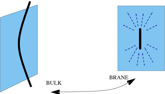
Surfaces can curve in the ambient manifold, whether or not that is itself curved (see figure 1). This is measured by the extrinsic curvature or second fundamental form, and is defined via
| (4) |
We can use the Riemann identity to get the Gauss-Codazzi relations
| (5) | |||||
| (6) |
In this last relation, we have the 5D Ricci tensor, which we can replace with the energy momentum tensor via Einstein’s equations; we also have a term which a second use of the Riemann identity allows us to write as a Lie derivative of the extrinsic curvature across the brane:
| (7) |
thus allowing us to rewrite the Gauss-Codazzi equations in terms of the extrinsic curvature and the energy momentum tensor:
| (8) |
Therefore, if we imagine our brane to be infinitesimally thin, having a distributional energy momentum, , then we see that the extrinsic curvature must have a jump across the brane. Integrating this out, we get the Israel equations:
| (9) |
Returning to the Randall Sundrum metric, (1), we see that
| (10) |
(where we are now dropping the distinction between the brane tangent space and the bulk tangent space, as the situation is physically clear). Using (9) we see that the brane has an energy-momentum tensor proportional to the metric on the brane:
| (11) |
Notice the very precise form of this energy momentum. First, because it is proportional to the intrinsic metric, this means that the brane has tension (rather than pressure) and this tension is exactly equal to its energy, . Thus the brane energy momentum has exactly the same form as a cosmological constant term on the brane. Second, the actual value of this tension is precisely related to the bulk cosmological constant:
| (12) |
This is sometimes referred to as the fine-tuned, or critical RS brane. As we will see later, this relation can be relaxed, leading to de Sitter or anti de Sitter RS branes (the latter of which are also known as Karch-Randall (KR) branes [22]).
3 Gravity in the Randall Sundrum model
Obviously the RS model can only describe our real universe if it correctly reproduces gravitational physics at experimentally tested scales. This means we have to be able to reproduce Einstein gravity in our solar system, and the standard cosmological model for our universe. While the Israel equations give us the general formalism for getting our braneworld metric, finding actual solutions can be a far trickier matter, as indeed finding a general solution of Einstein’s equations is a tricky matter! We therefore resort, as with standard gravity, to two main approaches:
Local Physics, or perturbation theory, and
“Big Picture” or geometry, finding exact solutions assuming symmetries.
In either case, we have to accept that gravity on the brane is a projection of the full higher dimensional nature of gravity, and is therefore a derived quantity.
3.1 Perturbation theory
In General Relativity (GR), classical perturbation theory involves perturbing the metric
| (13) |
around a given background solution. There are 3 main issues to bear in mind.
-
1.
is a perturbation and should therefore be “small”. What does this mean? In practise we have to be careful about our coordinate system, and always look at in a regular system. For the Schwarzschild solution for example, this means using Kruskal coordinates.
-
2.
Gauge freedom: GR has a large gauge group – physics is invariant under general coordinate transformations (GCT’s), and there are many gauge degrees of freedom in . For example, in 4D, has 10 independent components, but the graviton has only 2 physical degrees of freedom. Under a GCT
(14) hence
(15) and we can use this to make a choice of gauge. A common choice for relativists is the harmonic gauge
(16) and in vacuo we can also choose : the transverse tracefree (TTF) gauge. Note that this does not uniquely specify the gauge, e.g. gives an allowed gauge transformation.
-
3.
Finally, we need the perturbation of the Ricci tensor:
(17) often called the Lichnerowicz operator.
The simplest way to perturb the brane system is to take a GN system, in which the brane stays at :
| (18) |
The remaining gauge freedom allowed is
| (19) |
We can now input the purely 4D perturbation into the Lichnerowicz operator, and after some algebra, the perturbation equations reduce to:
| (20) | |||||
| (21) | |||||
| (22) |
where brane indices are raised and lowered with , and we allow for a matter perturbation confined to the brane:
| (23) |
It is easy to see the RS gauge is only consistent for vacuum perturbations, and that the zero modes have the behaviour (the graviton [5, 26]) and (the radion [27]).
A complete set of solutions to the free equations is readily found to be with
| (24) |
where , from which we can construct the Green’s function:
| (25) |

This has the structure of a zero mode (the part proportional to ), and a continuum of KK states. This is seen more clearly by looking at the restriction to a perturbation in the brane induced by a particle on the brane, for which
| (26) |
However, we have to remember that the RS gauge is only consistent in the absence of sources; in the presence of sources we have to fix the trace of the perturbation to satisfy the Lichnerowicz equation. Strictly speaking, we take the general metric perturbation, , and decompose it into its irreducible components with respect to the 4D Lorentz group (see [28]). This allows for a tensor (TTF) mode, a vector, and two scalars in general:
| (27) |
On shell, it can be shown that this reduces (up to purely 4D gauge transformations) to the following expression
| (28) |
which physically corresponds to the TTF 4D tensor , and a scalar, , which can be interpreted as a bending of the brane with respect to an observer at infinity [25] (see figure 2). This brane bending term couples to the trace of the energy momentum perturbation on the brane via (20), which implies a 4D equation for :
| (29) |
Solving (22), and pulling all this information together, we can now write the solution on the brane:
| (30) |
At mid to long range scales on the brane, the zero-mode dominates the integral and so we get:
| (31) |
Thus, if we identify as the 4D Newton constant, we have precisely 4D perturbative Einstein gravity with the correct tensor structure.
The effect of the massive KK modes on the Newtonian potential is also easily extracted using asymptotics of Bessel functions:
| (32) |
To see how these feed into corrections to Einstein gravity, consider the effect of a point mass source :
| (33) |
giving
| (34) |
Note this is in homogeneous gauge; transforming to the area gauge (where the area of 2-spheres is ) we have to leading order in :
| (35) |
We can visualize RS gravity as lines of force spreading out from the brane, but being “pushed back” by the negative bulk curvature. At small scales, the lines of force leave the brane and gravity is 5D and weaker. At larger scales, the bulk curvature bends the lines of force back onto the brane, and so gravity returns to being a 4D force law. (See figure 3.)

This is weak gravity, but what about strong gravity, such as black holes or cosmology?
3.2 Cosmology
For a cosmological brane, we have to ask whether there are surfaces of lower dimensionality which have the interpretation of an expanding universe. Recall that in standard cosmology, homogeneity and isotropy give a simple model of the universe in which everything depends on a single scale factor .
| (36) |
where the spatial metric is a surface of constant curvature , and in which satisfies a simple first order Friedman equation
| (37) |
where is the energy density of the universe, typically modelled by a perfect fluid with some equation of state .
For the cosmological braneworld, homogeneity and isotropy will still imply a constant curvature spatial universe, but now our “scale factor” must depend not only on time, but on the distance into the bulk. The remaining part of the metric in the t,z directions can be made conformally flat (any two dimensional metric can always be written in a conformally flat form) and so we may write the overall geometry as [29]:
| (38) |
The rationale for this specific way of writing the scale factor becomes apparent once the Einstein equations are analyzed. Here, z is representing the bulk coordinate away from the brane, though it no longer corresponds to proper distance. The brane sits at , which can always be chosen to be the location of the brane. (The conformal transformation maintains the form of the metric while taking an arbitrary wall trajectory to .)
In addition, the presence of a cosmological fluid will alter the usual brane relation by adding additional energy, , to E , and subtracting pressure, , from the tension T . Thus our brane energy momentum will now be
| (39) |
If we now compute the bulk Einstein equations, the reason for writing the metric in the slightly unusual form (38) becomes apparent. Using the lightcone coordinates
| (40) |
the bulk equations are:
| (41) | |||||
| (42) | |||||
| (43) |
This system is completely integrable, giving, after a change of coordinates, the bulk solution111Although note that there is a special case , , which is a near horizon limit of a black hole metric and a critical point of the Einstein equations [30, 31].
| (44) |
which is clearly a black hole solution. The parameter is related to the mass of the bulk black hole via [32]
| (45) |
The change of coordinates results in a shift of the brane to
| (46) |
where is the proper time of a brane observer.
Thus our cosmological brane is a slice of a black hole spacetime [33, 34, 16, 29]. We can think of our brane as moving in the bulk, and as it moves through a warped background, the brane will experience contraction or expansion as the surrounding geometry contracts or expands. The Israel equations give the dynamical equations for the brane trajectory , which can be massaged into the familiar Friedman form:
| (47) |
(see [29] for details). For a critical RS brane, which has , this gives
| (48) |
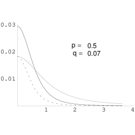
As might have been expected from the calculation of linearized gravity, the dominant form of this equation for small is indeed the standard Friedman equation. The effect of the brane shows up in the corrections, dubbed the non-conventional cosmology of the brane [34]. But most interesting from the point of view of these lectures is the presence of the last term, which is directly a result of the bulk black hole. This term, proportional to the mass parameter, takes the same functional form as a radiation source on the brane. Of course, the presence of the bulk black hole induces a periodicity in time in the Euclidean section, or, a finite temperature for any quantum field theory in the spacetime. Computing the background Hawking temperature of the black hole gives
| (49) |
where is the location of the event horizon, given by
| (50) |
For the case of the RS model, for which , this gives
| (51) |
where is now the comoving temperature on the brane. That this is suggestive of the Stefan law, , is not a coincidence, and is a theme we will pursue in the next section.
4 Black holes and holography
Both the linearized gravity result for an isolated mass and the brane cosmology metric suggest a somewhat deeper importance to braneworlds and black holes. The corrections to the Newtonian potential (33) in fact coincide precisely with the 1-loop corrections to the graviton propagator [35, 18], and the cosmological dark radiation term in the brane Friedman equation corresponds (up to a factor) to the energy density of a conformal field theory at the Hawking temperature of the black hole [16]. These clues, and analogies with lower dimensional branes, have led to the black hole holographic conjecture of Emparan, Fabbri and Kaloper [36] which states, loosely speaking, that if we have a classical solution to the RS model then we can interpret the braneworld as a quantum corrected 4D spacetime. In the case of the black hole, this would mean that we have a quantum corrected black hole.
The reason for putting forward such a conjecture is based in the adS/CFT conjecture [6] of string theory. In string theory, D-branes arise as the physical manifestation of open string Dirichlet boundary conditions. These D-branes are tangible objects carrying mass, Ramond-Ramond charge, and with worldvolume gauge theories to support the string endpoints [2]. Further, the supergravity solutions which correspond to the mass and charge of a particular type of D-brane must describe the same objects. The metric for a stack of coincident D3-branes is given by:
| (52) |
where is the string coupling and the string length scale. and are the cartesian metrics of the spaces respectively parallel and perpendicular to the brane, and is the radial coordinate in this latter space. We trust this supergravity solution in regions where the spacetime curvature is small, i.e. , where is the ambient spacetime curvature. Obviously, this will be true at large in (52), however, at large the effect of the branes is negligible. In order to trust the supergravity solution in regions where it is nontrivial, i.e. where , we require . In this case, we can effectively ignore the “” in the prefactor, and (52) is approximately:
| (53) |
This metric is adS. Thus, if we integrate over the , and identify
| (54) |
as the adS length scale, we can directly relate the near horizon régime of a stack of D3-branes with the RS model. Further, the 5D Newton constant will be given in terms of the 10D Newton constant and the volume of the 5-sphere by
| (55) |
Thus we can relate finite and classical quantities in our 5D Einstein theory, such as the adS curvature scale, , and the gravitational constant, , to quantum mechanical quantities such as , and , the number of D-branes. Indeed, we can potentially take a classical limit, , keeping our adS scale finite by simply simultaneously taking . On the other hand, this stack of D3-branes has a low energy worldvolume conformal field theory, and taking corresponds to the t’Hooft limit of the gauge theory. Since we have set , on the string side ensures that only this low energy sector remains. This is the essence of the adS/CFT correspondence, that certain strongly coupled conformal field theories are dual to string theory on certain anti-de Sitter spacetimes.
What does this mean for the RS model? As Gubser first noted, [16], brane cosmology with a black hole in the bulk has the appearance of a radiation cosmology from the brane perspective. From the Hawking temperature of the bulk black hole, the dark radiation term has the form (51), . On the other hand, calculating the energy of a CFT at finite temperature (at weak coupling) gives:
| (56) |
where is the coefficient for the trace anomaly in super Yang-Mills theory. Thus as ,
| (57) |
Clearly, if we identify , then we see that the classical bulk black hole has the effect on the brane of a thermal CFT at the comoving Hawking temperature of the black hole up to the conventional strong/weak coupling factor of . Note that the factor of in the definition of the 4D Newton’s constant is due to the fact that in adS/CFT we have a bulk on only one side of the boundary, whereas in physical braneworlds, we have bulk on each side of the brane. This effectively halves the brane tension, which is the key factor in the relation between the brane and bulk gravitational constants.
This rather physical picture of the interplay between the RS model and the adS/CFT conjecture is further fleshed out by the work of Duff and Liu [18], who note that the linearized corrections to the graviton propagator, calculated in (34), precisely agree with the 1-loop linearized corrections to flat space for a central mass [35]. These results are extremely suggestive that a fully nonlinear classical brane/bulk black hole solution would, from the brane point of view, correspond to a quantum corrected black hole. Indeed, it was this perspective that first led Tanaka to conjecture that a braneworld black hole must therefore be time-dependent, to agree with the thermal Hawking radiation from a Schwarzschild black hole [37]. Emparan, Fabbri and Kaloper then pointed out that the issue of time dependence is linked to the choice of quantum vacuum, and gave a comprehensive analysis of 3D brane black holes, together with options for the RS black hole.
Roughly, the picture is as follows. If we consider a closed universe with a bulk black hole, then the brane is precisely equidistant from the bulk black hole, and the radiation on the brane is precisely thermal. However, we could imagine displacing the brane slightly, which would introduce an inhomogeneity in the dark radiation on the brane. Moving one side of the brane even closer to the bulk black hole would then increase this distortion, and would (hopefully!) correspond to a collapsing shell of warm radiation on the brane. This could then form its own black hole, which from the bulk perspective would correspond to the brane actually touching the black hole. The brane would remain glued to the black hole for a while, but eventually would separate, which process would correspond to black hole radiation (see figure 4).
On the other hand, it is always possible that there does exist a static black hole solution, which asymptotically has the form of (35). Such a black hole would, according to EFK, necessarily have a singular horizon. This classical solution would be a 5D version of the C-metric [38], which is a solution representing two black holes accelerating away from each other. The black holes are being accelerated by two cosmic strings, one for each hole, which pull the black hole out to infinity. The exact purely gravitational solution has a conical deficit which can be smoothed out by a U(1) vortex [39], rendering the spacetime nonsingular apart from the central singularities of the black holes. It is then straightforward to slice this spacetime with a brane [40, 41] thus producing a 3D braneworld with a black hole. A positive tension brane retains the bulk without the cosmic string, hence these braneworld black holes do not need any further regularization. It may seem strange that a static black hole on the brane is accelerating, but it is no more unusual than the fact that we are in an accelerating frame on the surface of the Earth. Geodesics in the RS bulk actually curve away from the brane:
| (58) |
thus any observer glued to the brane is necessarily in an accelerating frame.
Moving up one dimension however changes the picture completely. The mathematics of the pure gravitational equations is now no longer amenable to analytic study, and no known C-metric exists. Even higher dimensional “cosmic strings” now have codimension three, and are strongly gravitating [42] with potentially singular geometries. We will now look at this problem in more detail.
5 Black hole metric
The first attempt to find a black hole on an RS brane was that of Chamblin, Hawking and Reall (CHR) [43], in which they replaced the Minkowski metric in (1) by the Schwarzschild metric (indeed, we can replace in (1) by any 4D Ricci-flat metric):
| (59) |
This is the only known exact solution looking like a black hole from the brane point of view. Unfortunately, it does not correspond to what we would expect for a brane black hole. If matter is confined to our brane, we would expect that any gravitational effect is localized near the brane. For a collapsed star, we would also intuitively expect that while the horizon might well extend out into the bulk, it too should be localized near the brane, and the singularity should not extend out into the bulk. The problem with the CHR black string, (59), is that it extends all the way out to the adS horizon, moreover, at this surface the black hole horizon actually becomes singular!
There is however another, more serious, problem with the CHR black string, and that is that it suffers from a classical instability [44]. Black string instabilities were first discovered in vacuum, [45], for the Kaluza-Klein black string:
| (60) |
This has a cylindrical event horizon, with entropy . On the other hand, assuming a KK compactification scale of , a 5D black hole of the same mass as the string (60) has an entropy of . Thus, for small enough masses relative to the compactification scale () a standard 5D black hole has higher entropy than the string, and thus the string should be either perturbatively or nonperturbatively unstable.
The existence of the instability can be confirmed by solving the Lichnerowicz equation
| (61) |
There is a subtlety involving the initial data surface, which must be taken to touch the future event horizon (the black hole generically forms from gravitational collapse), however, there is an unstable -mode with the form
| (62) |
(Note, this is written in Schwarzschild coordinates for convenience, but to check is small, use Kruskals.) This mode is physical, since any gauge degree of freedom would have to be purely 4D, thus satisfying a massless 4D Lichnerowicz equation, whereas this mode satisfies a massive 4D Lichnerowicz equation. The effect of the instability is to cause the horizon to ripple.
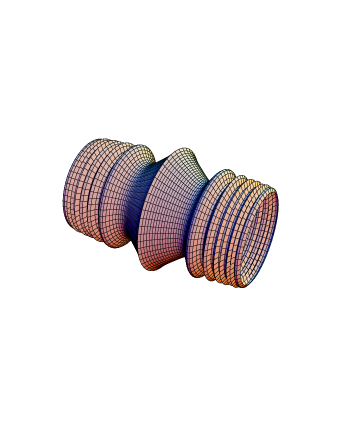
For the CHR black string, the presence of the bulk cosmological constant might be supposed to change the technicalities of this analysis, however, the crucial feature of the black string instability is that it is a purely 4D (massive) tensor TTF mode – i.e. it satisfies the RS gauge! If we work out the perturbation equations for the CHR black string background they have the particularly simple form:
| (63) |
This means we can simply take the standard KK instability and substitute the appropriate massive -dependent eigenfunction: , so that satisfies the equation of motion
| (64) |
where is the 4D Schwarzschild Lichnerowicz operator. In other words, we have the same 4D form for the instability, but a different -dependence appropriate to the RS background. Figure 5 shows the effect of the instability on the black string horizon, which now ripples with ever-increasing frequency towards the adS horizon.
It is tempting to link the existence of this instability to the thermodynamic instability of black holes to Hawking evaporation, however, the timescales have rather different behaviour. Not only that, but the instability is a dynamical process, and the amplitude of the instability, , is essentially arbitrary. The thermal radiation from a black hole however, is a quantum process with a well defined amplitude. To see the difference, note that for a black hole emitting radiation into states:
| (65) |
For the unstable black string, the mass function on the future horizon is given by an integral over the KK modes [46]
| (66) |
where is the ingoing Eddington Finkelstein coordinate, and the half life of the instability at , which is well approximated by (see the plots of vs. in [45]). Given this approximation, we can compare the rate of mass loss of the black hole to that by evaporation, by simply taking :
| (67) |
which clearly has a different dependence on and
It seems therefore that the holographic principle is not so straightforward to either confirm or implement, and reinforces the need for an exact solution. A natural method to try would be to take a similar approach as in cosmology: use the symmetries of the spacetime and construct the most general metric. Clearly we have spherical symmetry around the black hole, but we also have a time translation symmetry (assuming a static solution). This introduces an additional degree of freedom into the system, which can be parametrized as follows [47]:
| (68) |
The equations of motion then take the form
| (69) | |||||
| (70) | |||||
| (71) | |||||
| (72) |
where . This is clearly a fairly involved elliptic system, but unlike the cosmological equations, it is not integrable. What rendered the cosmological equations integrable was (43), of which (72) is the counterpart in this set of equations. The presence of the in (72) means that we can no longer use this to integrate up the other equations. It is possible to classify the separable analytic solutions, [47], however, none of these have the form expected of a brane black hole metric. The system can of course be integrated numerically, however, the typical method appropriate for elliptic systems (relaxation) is apparently extremely sensitive, and has difficulty dealing with radically different scales for the black hole mass and the adS bulk length scales. The consensus seems to be that nonsingular solutions representing static braneworld black holes exist for horizon radii of up to a few adS lengths [48] (see also [49]). However, there is no convincing demonstration of the existence of nonsingular static astrophysical brane black holes.
6 Approximate methods and solutions for brane black holes
Since we lack an exact solution, it is natural to attempt approximate methods to gain understanding of the system. There are two main approaches: One is to confine analysis to the brane, and to try to find a self-consistent 4D solution. This has the advantage of only dealing with one variable (the radius) thereby reducing the problem to a set of ODE’s. However, it has the clear disadvantage that it does not take into account the bulk spacetime, and therefore will not be closed as a system of equations – inevitably there will be some guesswork or approximation involved with terms that encode the bulk behaviour. The other main approach is to take a known bulk, such as the Schwarzschild-adS solution, and to explore what possible branes can exist. Within this method, the branes can either be taken as probe branes, i.e. branes which do not gravitationally back react on the bulk black hole, or as fully gravitating solutions to the Israel equations, which will therefore have restricted trajectories.
Other approaches not reviewed here include allowing for more general bulk matter, [50], which moves beyond the RS model being considered here. Also, the extension of brane solutions into the bulk, have been explored perturbatively [51], and as numerically [52].
6.1 Brane approach
The brane approach is based on the formalism of Shiromizu, Maeda and Sasaki (SMS) [53], who showed how to project the 5D Einstein-Israel equations down to a 4D brane system. The SMS method uses the fact that the RS braneworld has -symmetry, and writes (6) at using the bulk Einstein equations to replace the 5D Ricci tensor, and the Israel equations (9) to replace the extrinsic curvature:
| (73) |
using (23) to define . The only term that cannot be substituted by known quantities is the contraction of the Riemann tensor. Instead, SMS define an (unknown) Weyl term:
| (74) |
which is tracefree.
Using these substitutions, one arrives at a brane “Einstein” equation:
| (75) |
where the tensor is quadratic in :
| (76) |
Clearly these equations have an attractive simplicity, particularly if solving for an empty brane, however, it is important to note that the Weyl term (74) is a complete unknown, and depends on the details of the bulk solution.
For the case of the black hole however, one can use a method similar to that in brane cosmology, [54], to decompose the Weyl term into two independent pieces:
| (77) |
where is a unit time vector, a unit radial vector, and is here the purely spatial part of the braneworld metric. This renders the vacuum brane equations (75) rather similar to the Einstein equations with a gravitating perfect fluid: the Tolman Oppenheimer Volkoff (TOV) equations. Of course, and are complete unknowns, and do not not necessarily satisfy any conventional energy conditions, however, this notional similarity is very useful in understanding the physical system, and in fact allows us to derive useful insight into braneworlds stars, [55], such as the fact that the exterior of a collapsing star is not, in fact, static and Schwarzschild.
The vacuum equations have been solved in many special cases, for example, Dadhich et. al. [56], showed that there was an exact solution with having the form of a (zero mass) Reissner-Nordstrom metric on the brane. Other analytic solutions can be found by assuming a given form for the time or radial part of the metric [57, 58]. However, a useful approach to solving these equations is to take an arbitrary spherically symmetric metric, in which we allow for a general area functional for the 2-spheres, then apply an equation of state between and [59]:
| (78) |
The Einstein equations reduce to a two dimensional dynamical system from which it is relatively easy to extract general information about the system. Obviously, we do not expect that this unknown tensor will have such a simple equation of state as (78), however, just as in cosmology we approximate the energy momentum of the universe by various eras with fixed equations of state, it seems reasonable to approximate the near and far horizon behaviour by a fixed .
At large , we might expect the linearized solution (35) on the brane, which corresponds to . Closer to the horizon however, it is possible that could become very large and negative. There is in fact an exact solution for which displays features which are generic to solutions with (the tidal Reissner Nordstrom solution):
| (79) |
This solution has a null singularity at , the relic of an horizon, but also note that it actually has a ‘wormhole’, i.e. the area of 2-spheres surrounding the origin actually has a minimum value outside the horizon (for ), and is increasing as the horizon is approached. A sketch of a constant time surface is shown in figure 6.

It is tempting to conjecture that in fact any such static solution is singular, but while suggestive, these general arguments are not a proof, and investigations to determine the nature of the braneworld black hole horizon have been inconclusive [60].
6.2 Bulk approach
The other main approach which can yield insight into brane solutions is to simplify the problem by taking a known bulk, and exploring the possibilities for a brane solution with internal spherical symmetry. With this approach the bulk is now known (although rather rigidly fixed) and therefore the system has no ‘unknowns’. The first work in this area took the brane to be non-gravitating – a probe brane – and determined the general trajectories and dynamics of the brane [61, 62]. Although this work is not gravitationally self-consistent, it is important in particular because it gives insight into highly time dependent and complicated processes, and is to date the only available study of the process of a black hole leaving the brane. This has relevance for LHC black holes, as the main alternative to decay via Hawking evaporation is black hole recoil into the bulk, although the holographic point of view would argue these are indistinguishable [63].
In these lectures, we are mostly concerned with the gravitational properties of brane black holes, and so want to keep the brane at finite tension and have a consistent back reaction. This is a far more complicated and restrictive problem, however it is possible to obtain a linearized metric for a black hole that has left the brane [64]. This has the form of a shock wave of spherically symmetric outgoing radiation on the brane. For a full nonlinear analysis, we have to look for spherically symmetric branes embedded in a 5D Schwarzschild-adS spacetime using the Israel formalism. This leads to some interesting solutions, although the price to be paid is that the brane is no longer empty: we require energy momentum on the brane to source the gravitational field. This presentation is based on [65], but see also [66, 67].
The basic idea is to use the Israel equations with a bulk metric of the general Schwarzschild-adS form. The brane is spherically symmetric, with additional matter content corresponding to a homogeneous and isotropic fluid, in other words a braneworld TOV system. Note however that here there is an actual energy momentum source on the brane, in addition to the Weyl term (74) which is now specified from the brane embedding in the bulk metric:
| (80) |
For the brane trajectory, consistent with the symmetry, we take a general axisymmetric slice . Finally, for the energy-momentum tensor of the brane we take a general isotropic fluid source:
| (81) |
It turns out to be convenient to write the Israel equations in terms of ,
| (82) | |||||
| (83) | |||||
together with a conservation equation which determines T .
These equations can be completely integrated in terms of a modified radial variable
| (84) |
giving:
| (85) | |||||
| (86) | |||||
| (87) |
Finally the induced metric on the brane is
| (88) |
So far, this is a completely general (implicit) exact solution which depends on an integral of the bulk Newtonian potential . Although this is an exact solution, the actual properties of the brane depend on the specifics of the relation between and . Once this is determined, we have a solution describing a static, spherically symmetric distribution of an isotropic perfect fluid on the brane, i.e. a solution to the brane TOV system, and therefore a candidate for a brane “star”. The extent to which this is a physically realistic solution will depend on the energy and pressure profiles. Note that the profiles and represent the full brane energy momentum, and include the background brane tension. The relevant physical energy and pressure will be defined by
| (89) |
where is an appropriate background brane energy, which has to be identified on a case by case basis.
For a 5-dimensional adS bulk, , and the brane satisfies
| (90) | |||||
| E | (91) | ||||
| (92) |
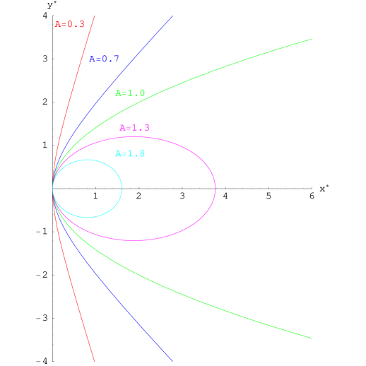
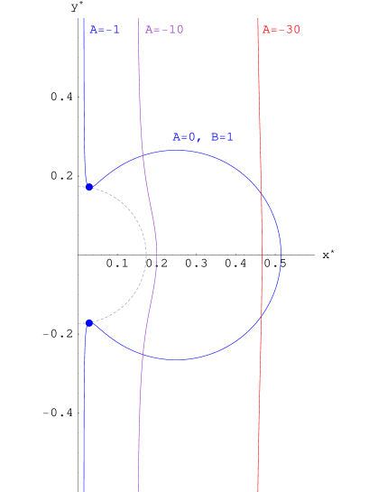
where , and in terms of the parameters in (85). These brane trajectories are conic sections classified by . For , the brane is a paraboloid with critical RS tension , (12). For , the brane is an ellipsoid (hyperboloid) with super- (sub-) critical tension. is a special case, corresponding to a subcritical Karch Randall brane and is a straight line. Figure 7 shows sample brane configurations for various values of the integration parameters and .
Notice that the energy density is constant, and requires to be positive. The tension on the other hand is clearly not constant unless . For the general brane we have a gravitating source composed purely of pressure! These branes clearly do not asymptote exact Randall-Sundrum or Karch-Randall branes. However, if and are large enough, the metric can be flat (or asymptotically (a)dS) over many orders of magnitude before the effect of the pressure kicks in.
It is also interesting also to look at a pure Schwarzschild bulk, , for which
| (93) | |||||
| (94) | |||||
| (95) |
where now , and in terms of the general solution (85). Note that by construction, these trajectories are strictly only valid outside the event horizon of the black hole, since the definition of the coordinate involves a branch cut there. In contrast to the adS case, E is not constant for these branes. For our solution to correspond to a brane star or black hole, we require E to be positive, and to increase towards the centre of the brane.
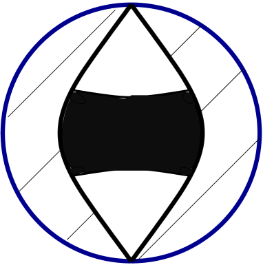
Looking at the large behaviour of (93), we see that the brane can only reach large if , otherwise the brane is either a bubble (enclosing the horizon or not, depending on and ) or an arc touching the horizon. In general, the brane touches the horizon at a tangent, and the pressure diverges, however, for one special case , the brane slices through the horizon passing on to the singularity. Some sample closed trajectories are shown in figure 8.

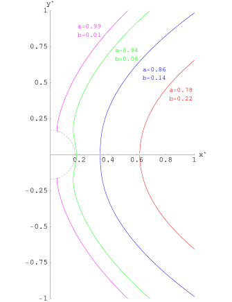
The most physically interesting Schwarzschild trajectories are those which tend to infinity, for which , see figure 9).
For these branes , and thus
| (96) |
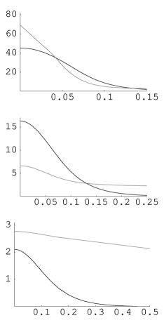
For , these branes have positive energy and pressure, uniformly decreasing as , and respectively. If , the brane never touches the horizon and the pressure remains everywhere finite. Thus these correspond to asymptotically empty branes with positive mass sources. Plotting the energy and pressure for the brane shows that this does indeed correspond to a localized matter source, with the peak energy density dependent on the minimal distance from the horizon (see figure 10).


The central energy and pressure can be readily calculated from this minimal radius, :
| (97) |
which shows that the central pressure diverges as . This is analogous to the divergence of central pressure in the four-dimensional TOV system, which is indicative of the existence of a Chandrasekhar limit for the mass of the star.
In these spacetimes, there is no actual black hole in the bulk, since it is the bulk to the right of the brane that is retained. Rather, it is the combination of the bulk Weyl curvature and the brane bending which produces the fully coupled gravitational solution. As the brane moves away from the horizon, the brane matter source spreads out, but the total mass changes very little, and is determined by the bulk black hole mass. The limit on mass is therefore not a true Chandrasekhar limit, but more a statement about an upper bound on the concentration of matter. The real reason there is no absolute upper bound is because, unlike the RS system with an adS bulk, gravity on the braneworld is not localized, nor is it four-dimensional. Computing the induced metric on the brane in fact shows that it is the projection of the 5D Schwarzschild metric on the brane.
6.2.1 Braneworld Stars : A Schwarzschild-adS Bulk
For the true braneworld star, the appropriate bulk is expected to be Sch-adS bulk: . Here has an exact analytic expression
| (98) |
with the black hole horizon, (50), and is defined as
| (99) |
Since the Randall Sundrum model is a brane in adS spacetime, we expect that any consistent brane trajectories in Sch-adS will potentially correspond to brane stars or black holes. It is worth stressing that these solutions will not just be brane solutions, but full brane and bulk solutions, since the full Israel equations for the brane have been solved in a known bulk background.
From (86) the background brane tension is defined as
| (100) |
For large enough , the geometry is dominated by the cosmological constant, therefore the pure adS solutions will be good approximations to any trajectories for large . Also, if , i.e. if the black hole is much smaller than the adS scale, we expect that in the vicinity of the horizon the Schwarzschild solutions will be good approximations for the brane, therefore for small mass black holes, we might expect brane trajectories to be well approximated by some combination of Schwarzschild and adS branes. Because the -coordinate has been zeroed at infinity (for easy comparison with the pure adS limit) the range of in Sch-adS is finite, and decreases sharply with increasing . This suggests that trajectories in large mass Sch-adS black hole spacetimes are more finely tuned, and possibly more restricted than in small mass black hole spacetimes.
Like adS spacetime, the Sch-adS trajectories can be classified according to whether they asymptote the adS boundary at nonzero , at , or do not reach the boundary at all, i.e. are closed bubbles. These correspond to subcritical, critical, or supercritical branes (, , and ) respectively. A sample of brane trajectories is shown in figure 11.

The supercritical branes are qualitatively similar to the pure Schwarzschild case, however, it is interesting to note that in each case there exists a purely empty spherical brane, equidistant from the horizon. This corresponds to the Einstein static universe [30], which from the brane perspective is a closed universe stabilized by a combination of the cosmological constant (the brane is supercritical) and the CFT dark radiation term. Using the holographic intuition, we might expect that by displacing this universe slightly we could mock up the start of gravitational collapse, however, a quick computation shows that displacing the brane relative to the black hole slightly sets up an energy deficit on the part of the brane closer to the black hole!
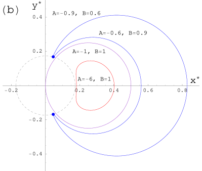
In the case of critical branes, , which means that the brane trajectories asymptote the adS boundary at exactly . The branes are thus open, and may or may not touch the black hole horizon depending on the exact values of the parameters and . If
| (101) |
the trajectory remains away from the horizon, otherwise it will touch the horizon and have a pressure singularity. A sample of critical trajectories in a Sch-adS background is shown in figure 12(a).
For branes that avoid the horizon the energy density is positive, peaking at the center, and dropping rapidly to the background value, undershooting it very slightly to form an underdense region at very large . The pressure also reaches its maximum value at the center, but is uniformly decreasing with , at a much slower rate, consistent with the pressure excess observed for the pure adS branes. Apart from this pressure excess, the other main difference with pure Schwarzschild trajectories, is that the brane matter can no longer universally satisfy the Dominant Energy Condition (DEC) (). In pure Schwarzschild, the DEC is satisfied except for branes which skirt extremely close to the horizon, where the local Weyl curvature causes the pressure to diverge. This phenomenon is also observed for the Sch-adS branes skimming close to the horizon, however, as we increase the central energy dominates the pressure for only a finite range of before once again dropping below the pressure. This is because the further we move away from the horizon the adS curvature becomes more important, and for pure adS branes, the effect of the adS curvature is to induce a pressure excess. In figure 12(b), the energy density and pressure of the matter on the brane is shown for a sequence of critical branes in a Sch-adS background displaced an increasing distance from the horizon.
Subcritical branes are largely similar to critical branes, and correspond to open trajectories that asymptote the adS boundary, although at nonzero in this case. The same bound as before, i.e. whether , will determine whether the brane terminates on the event horizon or remain on the RHS of it. The energy density and pressure profile in this case is again similar to the one found for critical branes. Once again, for a large family of parameters and , solutions with a positive energy excess at the center of the brane may be easily found.
One special subcritical trajectory found in the pure adS case was the Karch-Randall trajectory, . We can extend this to Sch-adS obtaining
| (102) |
however, since for a positive energy trajectory, this has , and hence the energy density is always increasing with . Thus, whether or not these trajectories terminate on the horizon, they always correspond to energy deficits on the brane, and hence negative mass sources from the point of view of a brane observer.
To sum up: we can get static solutions to the brane-TOV equations, and hence static brane stars. Unfortunately, the restricted form of the bulk leads to unphysical asymptotic behaviour away from the star in the form of a pressure excess. One possible way of removing this would be to perturb the bulk slightly at large to remove this excess. However, another interesting route to explore is to make the trajectory time dependent. In [55] it was argued that the spacetime surrounding a collapsing brane star would be time dependent even though it was vacuum. In fact, the RS trajectory is time dependent when written in global adS coordinates, which of course are the coordinates used for the Schwarzschild-adS metric:
| (103) |
The RS wall is oscillatory because the spherical coordinates are the universal covering space of adS, and so the ‘wall’ is actually an infinite family of walls, each in the local patch covered by the horospherical coordinates. Since is a geodesic of the spherical adS spacetime, the image of in the Randall-Sundrum spacetime, which is a hyperbola, will be a geodesic in the RS spacetime. Therefore, if we put a black hole at , it should look like a particle in the RS spacetime, at least to a first approximation.
We can generalize the brane trajectory to , and compute the corresponding time dependent versions of (82,83), then find the energy momentum source required on the brane. The idea is that a time dependent brane solution would describe a black hole forming from the collapse of radiation, and its subsequent evaporation, thus it is not clear whether we should expect a pure brane energy momentum solution; rather, a solution corresponding to the collapse of matter on the brane is perhaps more physically realistic. The energy momentum of a surface slicing the Sch-adS spacetime is given by the Israel junction conditions as:
| (104) |
Clearly, since the trajectory is time dependent, the energy momentum will also be time dependent, however, since the largest effect of the bulk black hole will be represented by the slice of the braneworld – the point of closest proximity – we evaluate the energy momentum at . For a pure RS trajectory, the black hole causes the energy of the brane to decrease from its critical value, whereas both the radial and azimuthal tension increase, thus the brane matter violates all the energy conditions! However, this was not unexpected as the RS trajectory was not modified, and the main feature of the static brane solutions was that they responded to the bulk black hole by bending. Indeed, in a definitive brane gravity paper, [25], Garriga and Tanaka showed that a crucial part of obtaining four dimensional Einstein gravity (i.e. with the correct tensor structure) was what could be interpreted as a brane bending term. As shown in section 3, the effect of matter on the brane is to “shift” the brane with respect to the acceleration horizon in the bulk (29). Clearly then, if a black hole forms on the brane, we would expect the brane to respond to this matter by bending.
A shift in the position of the brane corresponds to , and trying a test function:
| (105) |
gives the behaviour shown in figure 13 for a range of of and . (The brane bending of corresponds approximately to .)

The brane energy momentum in figure 13 satisfies the WEC, however, not the DEC. If the brane is bent instead towards the black hole the brane WEC is violated. The excess of angular pressure is somewhat similar to the pressure excesses in the static brane trajectory, however, unlike the static trajectories, here the black hole actually is in the bulk, hence these are true candidates for black hole recoil into the bulk.
6.2.2 The interaction of black holes and branes
The main motivating factors for obtaining a time-dependent braneworld black hole are to gain insight into the back-reaction of Hawking radiation on a quantum corrected four-dimensional black hole, and to understand the process of black hole recoil from a braneworld. Presumably the time-dependent process will be some perturbed version of a time-dependent brane trajectory in five-dimensional Sch-adS spacetime. By allowing the brane to intersect the bulk black hole horizon, this would appear to describe black hole formation and evaporation via transport of a bulk black hole to the brane, and subsequent departure back into the bulk. When the brane hits the black hole, we might expect some part of it will be captured by the black hole, and will therefore remain behind the event horizon even when the black hole has left the brane, effectively having been chopped off from the rest of the brane. This feature is seen in the probe brane calculations of [62], and we expect this to hold in the case of a fully gravitating brane. In support of this, we can appeal to the case of a cosmic string interacting with a black hole, where early work indicated that strings would be captured [68], and via self-intersection would leave some part behind in the black hole. Gravitational calculations of the fully coupled string/black hole system show explicitly how this ties in with the thermodynamic process of string capture and black hole entropy [69].

The basic idea is that once part of a brane has fallen into the event horizon of a black hole, it can no longer leave. Thus, if the brane has enough kinetic energy to subsequently pull away from the black hole, the price it must pay is to leave behind the part that has already been captured, see figure 14 [62]. However , RS braneworlds are not probe branes, but are strongly gravitating objects, and therefore any dynamic process must also be gravitationally consistent. From the gravitational point of view, when the black hole captures part part of the brane and excises it from the whole, the black hole must increase in mass. This interplay is seen particularly clearly in the related case of the cosmic string [69], where a cosmic string piercing a black hole alters the thermodynamic relations between mass, entropy and temperature. In that case, the (static) results are entirely consistent with the black hole having captured a length of cosmic string, thus increasing its mass. Just as in the cosmic string case, the capture of the codimension 1 RS brane by the black hole will turn out to be important in establishing the thermodynamic viability of the black hole recoil process.
At a first pass, it seems that in fact black hole recoil cannot occur in RS braneworlds due to a simple entropy argument [70]. In 5D, entropy is proportional to , hence two black holes of mass have less entropy than a single black hole of mass . However, this argument is both incorrect in the evaluation of the entropy, and misses additional contributory factors such as brane bending and brane capture by the black hole.
To get a better estimate, first note that entropy is proportional to horizon area/volume, which for Sch-adS is not simply related to the mass, but also to the adS scale:
| (106) |
Note that if , then the entropy of two black holes of mass will in fact be greater than that of a single black hole of mass . Therefore, at least from this rather approximate entropic argument, black hole recoil would seem to be problematic only for small black holes. On the other hand, in any dynamic process, we must take into account the capture of part of the brane by the black hole. Consider the idealized situation where we have a black hole intersecting the brane along its equator, in this case, a volume of of brane has been captured by the black hole, with a corresponding mass of
| (107) |
Adding this mass to the recoiled black holes results in an order of magnitude improvement to the bound on coming from the entropy: for , the entropy of the recoiled black holes becomes greater than that of the black hole on the brane.
Finally however, the most crucial factor is the brane bending. For a mass on the brane, the brane bends away from the acceleration horizon, and (as we have seen) the brane tends to bend away from the black hole. This effect will be most marked for the smallest black holes. We therefore have to correct the entropy argument to allow for the fact that more than half of the black hole horizon is sticking out into the bulk. (See figure 14.) Ignoring the effect of the captured brane increasing the mass, a quick calculation shows that the effective mass of the intermediate black hole stuck on the brane is
| (108) |
where is the minimal angle at which the brane touches the event horizon (assuming the black hole approaches from ). For , a rather modest amount of brane bending, the entropy of the recoiled black holes is always greater.
It is important to note that these arguments use the standard entropy of the isolated Sch-adS black hole. In other words, they assume a static solution with an event horizon at . Clearly in the time-dependent spacetime there is some question about whether this approximation is valid, and entropy arguments should be used with caution, nonetheless, for small black holes, where we might expect them to be more reliable, taking into account brane bending and fragmentation shows that it is by no means entropically preferred for a black hole to stick to the brane.
7 Outlook
As we have seen, the problem of braneworld black hole solutions is rather complex, and extremely interesting. The holographic principle puts forward the tantalizing prospect that if we can find a classical brane black hole solution (be it time dependent or static) then this gives us invaluable information about the quantum corrected black hole. The failure to find a classical solution so far can therefore be reinterpreted as the difficulty of consistently quantizing gravity. Yet the picture is not quite so clear. There have been several attempts to solve the brane black hole system numerically, [49], but as yet no unequivocal result. As we have seen, finding classical solutions directly is extremely difficult, and the only progress that has been made is partial, either by ignoring the bulk, or by relaxing the restrictions on the brane.
One interesting possibility, discussed in [71], is that the holographic principle is in fact not applicable to the RS model, and that the lack of an exact solution is unrelated to any problem of quantum gravity. Fitzpatrick, Randall and Wiseman (FRW) suggest that it is not appropriate to use the adS/CFT conjecture, as this refers to a quantum field theory at strong coupling, and the relation between the classical bulk solution and the quantum corrected brane solution requires the relation (55) where the classical effect is related to the full degrees of freedom of the field theory. Since the field theory is strongly coupled, it is not obvious that we will indeed have access to all the states in all cases. For example, we do not see quarks or gluons outside the nucleus, so why should we expect to access the full range of states far away from a black hole?
Without an exact solution, there is no way of exploring which of these insights, the holographic picture of EFK discussed in section 4, or the gluon analogy of FRW, is correct. FRW are of the opinion that there does exist a nonsingular, static braneworld black hole solution, and proposed the CHR black string as a counterexample to the holographic conjecture. The main problem with this solution is that to render it stable a second brane is required in the bulk. This corresponds to an infra-red cut-off in the CFT, and it is by no means clear how this additional complication affects the holographic argument.
There is however another option for exploring the physics of braneworld black holes, and that is to move to the Karch Randall set-up [22]. The KR brane is slightly de-tuned from the critical RS value, and is sub-critical, with an effective negative cosmological constant residing on the brane. KR branes are thus adS slicings of adS. From the holographic point of view, this complicates the picture, as we are no longer in the near horizon limit of a stack of D3-branes, however, the KR brane can possibly be related to a defect CFT dual to the intersection of a probe D5 brane with a stack of D3 branes [72]. The advantage of considering this slightly detuned situation is that black holes in adS can be thermodynamically stable [73], and therefore the back reaction due to Hawking radiation can, in principle, be computed. On the other hand, the adS black string in adS becomes stable once the mass is sufficiently high [74], which has been argued to be dual to the Hawking-Page transition [75]. Thus, for large mass black holes on the KR brane, we can perform a direct comparison between the strong coupling holographic back reaction, and the weak coupling Hawking radiation back reaction.
Such a comparison was made in [76] using Page’s heat kernel method [21] for approximating the radiation back reaction. The physical set-up is that we have two KR branes stretching through the bulk, each with positive tension, and each cutting off the boundary of adS, hence each providing a UV cutoff CFT. The black string stretches between the two branes, and for large enough mass is stable (see figure 15):
| (109) |
where , with being the location of the KR branes, is the 4D adS curvature scale.
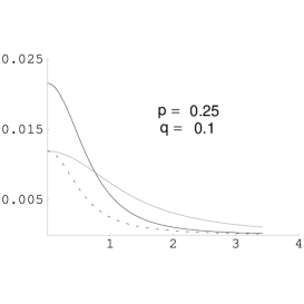
Restricting ourselves to a single brane, the geometry is that of 4D Sch-adS, and we can perform a standard weak coupling computation of the energy momentum tensor of the Hawking radiation. Figure 16 shows the energy and pressure of the thermal bath produced by the black hole (see [76] for details). Notice how at large the energy and pressures asymptote the form of a cosmological constant.
On the other hand, we have a full branebulk classical solution, and we can directly compute the effective stress tensor on the brane. It is clear before starting however, that this will not have the form of figure 16, as these varying energies and stresses will backreact on the spacetime to give a modification of the Sch-adS solution, whereas the classical solution is pure Sch-adS. On the other hand, although this is the classical brane solution, that does not mean that there is no back reaction on the brane energy momentum. In fact, the correction to the brane energy momentum is interpreted via the conventional 4D Einstein equation. From the brane point of view, we are unaware of the extra dimension, and therefore we interpret any deviation from the standard Einstein equation as additional energy momentum. Thus, while our KR brane energy momentum must have the form of a cosmological constant, it is possible that this is renormalized from the expected bare value.
To see how this works, let the tension of the KR brane be
| (110) |
where is the bare tension on the brane. On the other hand, the actual 4D cosmological constant is given by
| (111) |
Note that in this case, the 4D gravitational constant is not labelled as , since the relation between the brane and bulk gravitational constant is dependent on the brane tension, not the background adS curvature [77], and is altered from the critical RS relation:
| (112) |
From the definition of and (110,112), the value of the bare tension is:
| (113) |
Therefore, since the ‘expected’ value of the cosmological constant is , we can compute the correction to the brane energy momentum as:
| (114) |
This is the precise (classical) braneworld result. We can obtain the holographic renormalization result [78], by taking the limit as the brane approaches the boundary, or by approaching the critical RS limit . As , we get
| (115) |
which agrees with the strong coupling holographic result [76], up to the expected factor of two which arises from the braneworld set-up having two copies of the bulk, one on each side of the brane.
It is intriguing that the black hole apparently does not radiate in the strong coupling picture. This is a direct consequence of the fact that the bulk spacetime is foliated by conformal copies of the Schwarzschild-adS black hole. This ‘translation invariance’ means that the classical KK graviton modes are not excited in the background solution, and geometrically the only possibility is renormalization of the cosmological constant. It is possible that the black string solution is not the correct black hole metric candidate, however, one might expect that for brane black holes with , there is a unique stable regular black hole geometry, which this solution is.
Thus, the KR black string provides a counterexample to the expectation that a classical braneworld black hole corresponds to a quantum corrected 4D black hole. There are of course many caveats to this claim. Clearly the KR brane is not the near horizon limit of a stack of pure D3-branes, and therefore we do not expect the CFT to be a simple SYM. However, the fact that the renormalization of the stress tensor is proportional to , yet vanishes in the critical RS limit is supportive of the arguments of [71]. Obviously this debate is far from over! (See [79] for some recent work.)

Hopefully these lectures have given an insight into the complex and fascinating topic of braneworld black holes. However the field develops over the next few years, there are sufficient puzzles and unanswered questions to ensure that it will continue to be an active and exciting area.
Acknowledgments.
I would like to thank Lefteris Papantonopoulos for inviting me to such a lovely school, and also my collaborators throughout the years but in particular Simon Creek, Yiota Kanti, Bina Mistry, Simon Ross, Richard Whisker and Robin Zegers. This work was partially supported by the EU FP6 Marie Curie Research & Training Network ”UniverseNet” (MRTN-CT-2006-035863)References
-
[1]
V. A. Rubakov and M. E. Shaposhnikov,
Phys. Lett. B 125, 139 (1983).
V. A. Rubakov and M. E. Shaposhnikov, Phys. Lett. B 125, 136 (1983).
K. Akama, Lect. Notes Phys. 176, 267 (1982). [arXiv:hep-th/0001113]. -
[2]
J. Dai, R. G. Leigh and J. Polchinski,
Mod. Phys. Lett. A 4, 2073 (1989).
J. Polchinski, Phys. Rev. Lett. 75, 4724 (1995) [arXiv:hep-th/9510017]. -
[3]
P. Horava and E. Witten,
Nucl. Phys. B 475, 94 (1996).
[arXiv:hep-th/9603142].
A. Lukas, B. A. Ovrut, K. S. Stelle and D. Waldram, Phys. Rev. D 59, 086001 (1999) [arXiv:hep-th/9803235]. -
[4]
N. Arkani-Hamed, S. Dimopoulos and G. Dvali,
Phys. Lett. B429, 263 (1998)
[hep-ph/9803315].
N. Arkani-Hamed, S. Dimopoulos and G. Dvali, Phys. Rev. D 59, 086004 (1999) [hep-ph/9807344].
I. Antoniadis, N. Arkani-Hamed, S. Dimopoulos and G. Dvali, Phys. Lett. B 436, 257 (1998) [hep-ph/9804398]. -
[5]
L. Randall and R. Sundrum,
Phys. Rev. Lett. 83, 3370 (1999)
[arXiv:hep-ph/9905221].
L. Randall and R. Sundrum, Phys. Rev. Lett. 83, 4690 (1999) [arXiv:hep-th/9906064]. - [6] J. M. Maldacena, Adv. Theor. Math. Phys. 2, 231 (1998) [Int. J. Theor. Phys. 38, 1113 (1999)] [arXiv:hep-th/9711200].
-
[7]
G. W. Gibbons and D. L. Wiltshire,
Annals Phys. 167, 201 (1986)
[Erratum-ibid. 176, 393 (1987)].
D. Garfinkle, G. T. Horowitz and A. Strominger, Phys. Rev. D 43, 3140 (1991) [Erratum-ibid. D 45, 3888 (1992)]. - [8] N. I. Shakura and R. A. Sunyaev, Astron. Astrophys. 24, 337 (1973).
-
[9]
D. Lynden-Bell,
Nature 223, 690 (1969).
J. Kormendy and D. Richstone, Ann. Rev. Astron. Astrophys. 33, 581 (1995). - [10] R. Schodel et al., Nature 419, 694 (2002).
-
[11]
A. C. Fabian, K. Iwasawa, C. S. Reynolds and A. J. Young,
Publ. Astron. Soc. Pac. 112, 1145 (2000)
[arXiv:astro-ph/0004366].
M. Gierlinski and C. Done, Mon. Not. Roy. Astron. Soc. 347, 885 (2004) [arXiv:astro-ph/0307333]. - [12] E. G. Gimon and P. Horava, “Astrophysical Violations of the Kerr Bound as a Possible Signature of String Theory,” arXiv:0706.2873 [hep-th].
-
[13]
S. B. Giddings and S. D. Thomas,
Phys. Rev. D 65, 056010 (2002)
[arXiv:hep-ph/0106219].
S. Dimopoulos and G. L. Landsberg, Phys. Rev. Lett. 87, 161602 (2001) [arXiv:hep-ph/0106295]. -
[14]
C. M. Harris, P. Richardson and B. R. Webber,
JHEP 0308, 033 (2003)
[arXiv:hep-ph/0307305].
C. M. Harris, M. J. Palmer, M. A. Parker, P. Richardson, A. Sabetfakhri and B. R. Webber, JHEP 0505, 053 (2005) [arXiv:hep-ph/0411022].
G. L. Landsberg, J. Phys. G 32, R337 (2006) [arXiv:hep-ph/0607297].
M. Cavaglia, R. Godang, L. Cremaldi and D. Summers, Comput. Phys. Commun. 177, 506 (2007) [arXiv:hep-ph/0609001]. - [15] P. Kanti, “Black Holes at the LHC,” arXiv:0802.2218 [hep-th].
- [16] S. S. Gubser, Phys. Rev. D 63, 084017 (2001) [arXiv:hep-th/9912001].
-
[17]
H. L. Verlinde,
Nucl. Phys. B 580, 264 (2000)
[arXiv:hep-th/9906182].
E. P. Verlinde and H. L. Verlinde, JHEP 0005, 034 (2000) [arXiv:hep-th/9912018]. - [18] M. J. Duff and J. T. Liu, Phys. Rev. Lett. 85, 2052 (2000) [Class. Quant. Grav. 18, 3207 (2001)] [arXiv:hep-th/0003237].
- [19] S. W. Hawking, Commun. Math. Phys. 43, 199 (1975)
- [20] P. Candelas, Phys. Rev. D 21, 2185 (1980).
- [21] D. N. Page, Phys. Rev. D 25, 1499 (1982).
- [22] A. Karch and L. Randall, JHEP 05 (2001) 008, hep-th/0011156.
- [23] W. Israel, Nuovo Cimento Soc. Ital. Phys. B 44, 4349 (1966).
-
[24]
D. Garfinkle and R. Gregory,
Phys. Rev. D 41, 1889 (1990).
B. Carter and R. Gregory, Phys. Rev. D 51, 5839 (1995) [arXiv:hep-th/9410095].
B. Carter, Int. J. Theor. Phys. 40, 2099 (2001) [arXiv:gr-qc/0012036]. - [25] J. Garriga and T. Tanaka, Phys. Rev. Lett. 84, 2778 (2000) [arXiv:hep-th/9911055].
-
[26]
A. Chamblin and G. W. Gibbons,
Phys. Rev. Lett. 84, 1090 (2000)
[arXiv:hep-th/9909130].
S. B. Giddings, E. Katz and L. Randall, JHEP 0003, 023 (2000) [arXiv:hep-th/0002091]. - [27] C. Charmousis, R. Gregory and V. A. Rubakov, Phys. Rev. D 62, 067505 (2000) [arXiv:hep-th/9912160].
- [28] C. Charmousis, R. Gregory, N. Kaloper and A. Padilla, JHEP 0610, 066 (2006) [arXiv:hep-th/0604086].
- [29] P. Bowcock, C. Charmousis and R. Gregory, Class. Quant. Grav. 17, 4745 (2000) [arXiv:hep-th/0007177].
- [30] L. A. Gergely and R. Maartens, Class. Quant. Grav. 19, 213 (2002) [arXiv:gr-qc/0105058].
- [31] Z. Keresztes and L. A. Gergely, “On the validity of the 5-dimensional Birkhoff theorem: The tale of a counterexample,” arXiv:0712.3758 [gr-qc].
- [32] R. C. Myers and M. J. Perry, Annals Phys. 172, 304 (1986).
-
[33]
H. A. Chamblin and H. S. Reall,
Nucl. Phys. B 562, 133 (1999)
[arXiv:hep-th/9903225].
N. Kaloper, Phys. Rev. D 60, 123506 (1999) [arXiv:hep-th/9905210].
P. Kraus, JHEP 9912, 011 (1999) [arXiv:hep-th/9910149]. -
[34]
P. Binetruy, C. Deffayet and D. Langlois,
Nucl. Phys. B 565, 269 (2000)
[arXiv:hep-th/9905012].
C. Csaki, M. Graesser, C. F. Kolda and J. Terning, Phys. Lett. B 462, 34 (1999) [arXiv:hep-ph/9906513].
J. M. Cline, C. Grojean and G. Servant, Phys. Rev. Lett. 83, 4245 (1999) [arXiv:hep-ph/9906523].
P. Kanti, I. I. Kogan, K. A. Olive and M. Pospelov, Phys. Lett. B 468, 31 (1999) [arXiv:hep-ph/9909481]; - [35] M. J. Duff, Phys. Rev. D 9, 1837 (1974).
- [36] R. Emparan, A. Fabbri and N. Kaloper, JHEP 0208, 043 (2002) [arXiv:hep-th/0206155].
- [37] T. Tanaka, Prog. Theor. Phys. Suppl. 148, 307 (2003) [arXiv:gr-qc/0203082].
- [38] W. Kinnersley and M. Walker, Phys. Rev. D 2, 1359 (1970).
-
[39]
D. M. Eardley, G. T. Horowitz, D. A. Kastor and J. H. Traschen,
Phys. Rev. Lett. 75, 3390 (1995)
[arXiv:gr-qc/9506041].
R. Emparan, Phys. Rev. Lett. 75, 3386 (1995) [arXiv:gr-qc/9506025].
S. W. Hawking and S. F. Ross, Phys. Rev. Lett. 75, 3382 (1995) [arXiv:gr-qc/9506020].
R. Gregory and M. Hindmarsh, Phys. Rev. D 52, 5598 (1995) [arXiv:gr-qc/9506054]. -
[40]
R. Emparan, G. T. Horowitz and R. C. Myers,
JHEP 0001, 007 (2000)
[arXiv:hep-th/9911043].
R. Emparan, G. T. Horowitz and R. C. Myers, JHEP 0001, 021 (2000) [arXiv:hep-th/9912135]. - [41] R. Emparan, R. Gregory and C. Santos, Phys. Rev. D 63, 104022 (2001) [arXiv:hep-th/0012100].
-
[42]
R. Gregory,
Nucl. Phys. B 467, 159 (1996)
[arXiv:hep-th/9510202].
R. Gregory, JHEP 0306, 041 (2003) [arXiv:hep-th/0304262]. - [43] A. Chamblin, S. W. Hawking and H. S. Reall, Phys. Rev. D 61, 065007 (2000) [arXiv:hep-th/9909205].
- [44] R. Gregory, Class. Quant. Grav. 17, L125 (2000) [arXiv:hep-th/0004101].
-
[45]
R. Gregory and R. Laflamme,
Phys. Rev. Lett. 70, 2837 (1993)
[arXiv:hep-th/9301052].
R. Gregory and R. Laflamme, Nucl. Phys. B 428, 399 (1994) [arXiv:hep-th/9404071]. - [46] A. Fabbri and G. P. Procopio, Class. Quant. Grav. 24, 5371 (2007), 0704.3728 [hep-th].
- [47] C. Charmousis and R. Gregory, Class. Quant. Grav. 21, 527 (2004) [arXiv:gr-qc/0306069].
- [48] H. Kudoh, T. Tanaka and T. Nakamura, Phys. Rev. D 68, 024035 (2003) [arXiv:gr-qc/0301089].
-
[49]
T. Shiromizu and M. Shibata,
Phys. Rev. D 62, 127502 (2000)
[arXiv:hep-th/0007203].
A. Chamblin, H. S. Reall, H. a. Shinkai and T. Shiromizu, Phys. Rev. D 63, 064015 (2001) [arXiv:hep-th/0008177].
T. Wiseman, Phys. Rev. D 65, 124007 (2002) [arXiv:hep-th/0111057]. -
[50]
P. Kanti and K. Tamvakis,
Phys. Rev. D 65, 084010 (2002)
[arXiv:hep-th/0110298].
P. Kanti, I. Olasagasti and K. Tamvakis, Phys. Rev. D 68, 124001 (2003) [arXiv:hep-th/0307201]. - [51] R. Casadio and L. Mazzacurati, Mod. Phys. Lett. A 18, 651 (2003) [arXiv:gr-qc/0205129].
- [52] N. Tanahashi and T. Tanaka, JHEP 0803, 041 (2008) [arXiv:0712.3799 [gr-qc]].
- [53] T. Shiromizu, K. i. Maeda and M. Sasaki, Phys. Rev. D 62, 024012 (2000) [arXiv:gr-qc/9910076].
- [54] R. Maartens, Phys. Rev. D 62, 084023 (2000) [arXiv:hep-th/0004166].
-
[55]
C. Germani and R. Maartens,
Phys. Rev. D 64, 124010 (2001)
[arXiv:hep-th/0107011].
M. Bruni, C. Germani and R. Maartens, Phys. Rev. Lett. 87, 231302 (2001) [arXiv:gr-qc/0108013]. - [56] N. Dadhich, R. Maartens, P. Papadopoulos and V. Rezania, Phys. Lett. B 487, 1 (2000) [arXiv:hep-th/0003061].
- [57] R. Casadio, A. Fabbri and L. Mazzacurati, Phys. Rev. D 65, 084040 (2002) [arXiv:gr-qc/0111072].
-
[58]
M. Visser and D. L. Wiltshire,
Phys. Rev. D 67, 104004 (2003)
[arXiv:hep-th/0212333].
K. A. Bronnikov, V. N. Melnikov and H. Dehnen, Phys. Rev. D 68, 024025 (2003) [arXiv:gr-qc/0304068].
T. Harko and M. K. Mak, Phys. Rev. D 69, 064020 (2004) [arXiv:gr-qc/0401049]. - [59] R. Gregory, R. Whisker, K. Beckwith and C. Done, JCAP 0410, 013 (2004) [arXiv:hep-th/0406252].
-
[60]
K. A. Bronnikov and S. W. Kim,
Phys. Rev. D 67, 064027 (2003)
[arXiv:gr-qc/0212112].
D. Karasik, C. Sahabandu, P. Suranyi and L. C. R. Wijewardhana, Phys. Rev. D 70, 064007 (2004) [arXiv:gr-qc/0404015]. -
[61]
V. P. Frolov, M. Snajdr and D. Stojkovic,
Phys. Rev. D 68, 044002 (2003)
[arXiv:gr-qc/0304083].
D. Stojkovic, JHEP 0409, 061 (2004) [arXiv:gr-qc/0409038]. -
[62]
A. Flachi and T. Tanaka,
Phys. Rev. Lett. 95, 161302 (2005)
[arXiv:hep-th/0506145].
A. Flachi, O. Pujolas, M. Sasaki and T. Tanaka, arXiv:hep-th/0601174. - [63] V. P. Frolov and D. Stojkovic, Phys. Rev. Lett. 89, 151302 (2002) [arXiv:hep-th/0208102].
- [64] R. Gregory, V. A. Rubakov and S. M. Sibiryakov, Class. Quant. Grav. 17, 4437 (2000) [arXiv:hep-th/0003109].
- [65] S. Creek, R. Gregory, P. Kanti and B. Mistry, Class. Quant. Grav. 23, 6633 (2006) [arXiv:hep-th/0606006].
- [66] S. S. Seahra, Phys. Rev. D 71, 084020 (2005) [arXiv:gr-qc/0501018].
- [67] C. Galfard, C. Germani and A. Ishibashi, arXiv:hep-th/0512001.
- [68] S. Lonsdale and I. Moss, Nucl. Phys. B 298, 693 (1988).
-
[69]
A. Achucarro, R. Gregory and K. Kuijken,
Phys. Rev. D 52, 5729 (1995)
[arXiv:gr-qc/9505039].
F. Bonjour, R. Emparan and R. Gregory, Phys. Rev. D 59, 084022 (1999) [arXiv:gr-qc/9810061]. - [70] D. Stojkovic, Phys. Rev. Lett. 94, 011603 (2005) [arXiv:hep-ph/0409124].
- [71] A. L. Fitzpatrick, L. Randall, and T. Wiseman, JHEP 11 (2006) 033, hep-th/0608208.
-
[72]
A. Karch and L. Randall,
JHEP 0106, 063 (2001)
[arXiv:hep-th/0105132].
O. DeWolfe, D. Z. Freedman and H. Ooguri, Phys. Rev. D 66, 025009 (2002) [arXiv:hep-th/0111135]. - [73] S. W. Hawking and D. N. Page, Commun. Math. Phys. 87, 577 (1983).
- [74] T. Hirayama and G. Kang, Phys. Rev. D 64 (2001) 064010, hep-th/0104213.
- [75] A. Chamblin and A. Karch, Phys. Rev. D 72, 066011 (2005), arXiv:hep-th/0412017
- [76] R. Gregory, S. F. Ross and R. Zegers, arXiv:0802.2037 [hep-th].
-
[77]
U. Gen and M. Sasaki,
Prog. Theor. Phys. 105, 591 (2001)
[arXiv:gr-qc/0011078].
R. Gregory and A. Padilla, Phys. Rev. D 65, 084013 (2002) [arXiv:hep-th/0104262].
A. Padilla, Phys. Lett. B 528, 274 (2002) [arXiv:hep-th/0111247]. - [78] S. de Haro, S. N. Solodukhin and K. Skenderis, Commun. Math. Phys. 217, 595 (2001) [arXiv:hep-th/0002230].
-
[79]
A. Fabbri and G. P. Procopio,
“The Holographic Interpretation of Hawking Radiation,”
arXiv:0705.3363 [gr-qc].
T. Tanaka, “Implication of Classical Black Hole Evaporation Conjecture to Floating Black Holes,” arXiv:0709.3674 [gr-qc].
L. Grisa and O. Pujolas, “Dressed Domain Walls and Holography,” arXiv:0712.2786 [hep-th].
A. Flachi and T. Tanaka, “Vacuum polarization in asymptotically anti-de Sitter black hole geometries,” arXiv:0803.3125 [hep-th].