Spatiotemporal instability of a confined capillary jet

Abstract

Recent experimental studies on the instability appearance of capillary jets have revealed the capabilities of linear spatiotemporal instability analysis to predict the parametrical map where steady jetting or dripping takes place. In this work, we present an extensive analytical, numerical and experimental analysis of confined capillary jets extending previous studies. We propose an extended, accurate analytic model in the limit of low Reynolds flows, and introduce a numerical scheme to predict the system response when the liquid inertia is not negligible. Theoretical predictions show a remarkable accuracy with results from the extensive experimental exploration provided.

I Introduction

An important number of advances in the understanding of the physics of the controlled formation of biphasic flows ($\it{i.e.}$ emulsions, aerosols, microbubble dispersions, wet foams, etc.) have come after the incorporation of spatiotemporal analysis in the dynamics of capillary jets. A general successful paradigm in such controlled formation mentioned is the co-flow of the two phases involved, where a first fluid stream from a given source, usually a capillary tube, is surrounded by a second immiscible fluid stream. Basically, the first fluid stream may exhibit two possible behaviors: (i) it gives up blobs (droplets or bubbles) of sizes comparable to the typical source dimensions (usually the tube outlet diameter), or (ii) it yields a continuous stream in the form of a capillary jet whose diameter becomes independent of the typical source dimensions. These system modes are usually referred to as “dripping” or “jetting”, respectivelyLei86b ; Lin89 ; Cla99 ; Sev02 ; Lin03 ; SB2006 ; AP06 . In this later case, after the capillary jet breaks up into droplets a distance of several diameters downstream of the source, the eventual output is a stream of droplets or bubbles whose size is commensurate with the jet diameter. When subject to flow under certain geometrical configurations (like flow focusing, Gan98 ; Anna:2003 ; Gar04 ) or electrohydrodynamic actions (electrospray, Clou89 ; Gan97a ), the first fluid stream can be reduced to the form of a steady jet of very small diameter compared to the typical size of the source. In general, producing a biphasic flow based on jetting offers very significant advantages over dripping because (i) a fixed geometry can be tuned to yield a wide range of selectable droplet sizes based on relative flow rates only, (ii) the resulting droplet sizes can be sometimes extremely small compared to the given geometrical dimensions of the processing device, and (iii) under certain parametrical circumstances, the droplet size distribution can exhibit a low size dispersion. Thus, for each device geometry, mapping the different behaviors mentioned in the parametrical space of operation becomes a fundamental engineering endeavor.

An extremely simple yet successful device to produce such controlled biphasic flows is a concentric capillary tube arrangementUtada:2005 ; Guillot2007 . Using such a geometry, a smaller diameter tube coaxially positioned inside of another wider confining tube releases a stream of a first fluid, usually a liquid, while a second fluid flows concentrically in the same axial direction (for example, see Fig. 1). This axisymmetric arrangement is rather common to many microfluidic systems. Very recently, Guillot et al.Guillot2007 have contributed very significantly to the physical knowledge of such a simple yet fundamental system, presenting a combined experimental and theoretical study with a remarkable degree of agreement at many parametrical regions, in spite that their theoretical model proposed assumed important simplifications: both the basic flow and its perturbations were averaged in the radial direction for both streams, and inertia was neglected through the whole study (justifiable in microfluidics). These simplifications naturally become shortcomings in some cases where predictions deviated from experiments. In this work, we aim to investigate whether an axisymmetric model which does not make use of these simplifications improves its predictive power over the simplified one. To do so, we split our study into two subsequent degrees of approximation to the real physics: firstly, we assume the perturbed flow three dimensional axisymmetric under negligible inertia, and secondly, we add inertia. The first study still admits analytical treatment in spite of the extremely complexity of the resulting mathematical expressions, which should be handled by a computer assisted algebraic manipulation ($\it{e.g.}$ Mathematica®), and the second study is numerically tackled. Our theoretical results are compared to an extensive collection of experiments, an important part of which is here presented for the first time. As expected, the theoretical agreement with experiments improves significantly. Still, some remaining disagreements are discussed in detail, possibly shedding some light on the dynamics of these flows for future studies.

II Mathematical Formulation

We studied the spatial response to small perturbations of an infinite cylindrical capillary liquid jet of radius $R_{1}$ confined in a cylindrical coaxial pipe of radius $R_{2}>R_{1}$. The liquid jet of density $\rho_{1}$ and viscosity $\mu_{1}$ is surrounded by another liquid of density $\rho_{2}$ and $\mu_{2}$. The governing equations are the incompressible Navier-Stokes equations in cylindrical coordinates, $(z,r,\theta)$, which are made dimensionless by using the radius of the jet, $R_{1}$, the velocity at the liquid-liquid interface, $U$, and inertia $\rho_{1}U^{2}$, as characteristic quantities. This problem admit an exact steady unidirectional solution which only depends on two dimensionless parameters; the viscosity ratio $\mu=\mu_{2}/\mu_{1}$ and the quotient between the pipe wall radius an the radius of the liquid jet, $R=R_{2}/R_{1}$. The velocity field $(U,V)$ of this basic solution is given by:

$$\begin{array}[]{ccccc}U_{1}(r)&=&1+\mu\displaystyle\frac{1-r^{2}}{R^{2}-1},&V_{1}(r)=0&\quad(0\leq r\leq 1),\\ U_{2}(r)&=&1+\displaystyle\frac{1-r^{2}}{R^{2}-1},&V_{2}(r)=0&\quad(1\leq r\leq R),\end{array}$$ (1)

where subscript $1$ ($2$) denote the inner (outer) liquid velocity fields. To study the stability of the flow, we will introduce a small unsteady axisymmetric perturbation in the velocity and pressure fields of the form,

$$\{u_{n}^{\prime},v_{n}^{\prime},p_{n}^{\prime}\}(r,z)=\{u_{n},v_{n},p_{n}\}(r)\exp\left[i(kz-\omega t)\right],\quad(n=1,2),$$ (2)

where $\omega$ is the dimensionless wave frequency, $k$ is the dimensionless wave number, $u$ and $v$ are the axial and radial velocities respectively, and $p$ is the pressure field. In addition to this, the radial position of the liquid-liquid interface is also perturbed in the form

$$r_{i}(z,t)=1+c_{o}\exp\left[i(kz-\omega t)\right],$$ (3)

where $c_{o}$ is the small amplitude of the perturbated interface ( $c_{o}<<1$).

Substituting the basic flow given by (1) and the perturbed one given by (2) and (3) into the Navier-Stokes equations and after linearizing we get the following set of equations:

$$iku_{n}+\frac{1}{r}\frac{\partial}{\partial r}(rv_{n}) = 0,$$ (4)

$$(-\omega i+ki)u_{n}+\frac{\partial U_{n}}{\partial r}v_{n}+ik\rho^{-\delta_{n2}}p_{n}-\left(\frac{\mu}{\rho}\right)^{\delta_{n2}}\frac{1}{Re}\left[\frac{1}{r}\frac{\partial}{\partial r}(r\frac{\partial u_{n}}{\partial r})-k^{2}u_{n}\right] = 0,$$ (5)

$$(-\omega i+ki)v_{n}+\rho^{-\delta_{n2}}\frac{\partial p_{n}}{\partial r}-\left(\frac{\mu}{\rho}\right)^{\delta_{n2}}\frac{1}{Re}\left[\frac{1}{r}\frac{\partial}{\partial r}(r\frac{\partial v_{n}}{\partial r})-k^{2}v_{n}-\frac{v_{n}}{r^{2}}\right] = 0,$$ (7)

$$(n=1,2)$$

where $\delta_{n2}$ is the Kronecker delta. In the above equations, $Re$ represents the Reynolds number of the inner liquid, defined as $Re=\rho_{1}UR_{1}/\mu_{1}$, and $\rho=\rho_{2}/\rho_{1}$ is the density ratio. Equations (4)-(7) must be solved subject to the following boundary conditions:

• At the axis, r=0, regularity conditions:

  $$v_{1}=0,\quad\frac{\partial u_{1}}{\partial r}=0.$$ (8)

• At the liquid-liquid interface, $r=1$, continuity of both the velocity filed and tangential stresses, and normal stresses balance with capillary forces which yield:

  $$v_{1}=v_{2},\quad u_{1} = u_{2},$$ (9)

  $$\frac{\partial u_{1}}{\partial r}-\mu\frac{\partial u_{2}}{\partial r}-ik(\mu v_{2}-v_{1}) = 0,$$

  $$p_{1}-p_{2}-\frac{2}{Re}\frac{\partial v_{1}}{\partial r}+\frac{2\mu}{Re}\frac{\partial v_{2}}{\partial r}+\frac{c_{o}}{We}(1-k^{2}) = 0,$$

  being, $We=\rho_{1}U^{2}R_{1}/\sigma$, the Weber number based on the inner liquid density, the radius and the velocity of the jet at the interface and the liquid-liquid surface tension $\sigma$.

• At pipe wall, $r=R$, no slip conditions are applied:

  $$v_{2}=u_{2}=0.$$ (10)

Finally, by making use of the linearized kinematic condition for the interface we get:

$$i\omega c_{o}-ik+v_{1}(r=1) = 0.$$ (11)

Here, we will carry out a spatiotemporal stability analysis, which entails assuming both the frequency $\omega$ and the wave number $k=k_{r}+ik_{i}$ as complex. Using a well established criterionSaarloos87 ; Saarloos88 ; Guillot2007 , we say that a mode is convectively unstable if its spatial growth rate, $-k_{i}$, and its group velocity, $c_{g}=\partial\omega/\partial k_{r}$, are both positive for some frequency range.

II.1 Creeping flow limit, $Re\to 0$.

System of equations (4)-(11) can be substantially simplified when viscous effect are dominant ($Re\to 0$). In this limit the stability problem is governed by the following equations:

$$iku_{n}+\frac{1}{r}\frac{\partial}{\partial r}(rv_{n}) = 0.$$ (12)

$$ik\hat{p}_{n}-\mu^{\delta_{n2}}\left[\frac{1}{r}\frac{\partial}{\partial r}(r\frac{\partial u_{n}}{\partial r})-k^{2}u_{n}\right] = 0,$$ (13)

$$\frac{\partial\hat{p}_{n}}{\partial r}-\mu^{\delta_{n2}}\left[\frac{1}{r}\frac{\partial}{\partial r}(r\frac{\partial v_{n}}{\partial r})-k^{2}v_{n}-\frac{v_{n}}{r^{2}}\right] = 0.$$ (15)

$$(n=1,2)$$

Here, $\hat{p}=Re\cdot p$ is the re-scaled pressure amplitude.

• At the axis, r=0:

  $$v_{1}=0,\quad\frac{\partial u_{1}}{\partial r}=0.$$ (16)

• At the liquid-liquid interface, $r=1$:

  $$v_{1}=v_{2},\quad u_{1} = u_{2},$$ (17)

  $$\frac{\partial u_{1}}{\partial r}-\mu\frac{\partial u_{2}}{\partial r}-ik(\mu v_{2}-v_{1}) = 0,$$

  $$\hat{p}_{1}-\hat{p}_{2}-2\frac{\partial v_{1}}{\partial r}+2\mu\frac{\partial v_{2}}{\partial r}+c_{o}(1-k^{2})/Ca = 0,$$

  where now, $Ca=We/Re$, is a capillary number.

• At pipe wall, $r=R$:

  $$v_{2}=u_{2}=0.$$ (18)

The linearized kinematic equation for the interface reads:

$$i\omega c_{o}-ik+v_{1}(r=1) = 0.$$ (19)

Observe that while the complete problem is governed by five dimensionless parameters $\rho$, $\mu$, $Re$, $We$ and $R$, the creeping flow limit is governed by just three, $\mu$, $Ca$ and $R$.

II.2 Numerical scheme for the complete system

It proves convenient to rewrite Equations (4)-(11) in the form

$$[\mathbf{L_{1}}+k\mathbf{L_{2}}+\frac{k^{2}}{Re}\mathbf{L_{3}}]\mathbf{S}=0\,,$$ (20)

where $\mathbf{L_{1}}$, $\mathbf{L_{2}}$, $\mathbf{L_{3}}$ and $\mathbf{L_{3}}$ are complex matrices which depend on $r$, $\rho$, $\mu$ and $\omega$ and where ${\bf S}=[u_{1}(r),v_{1}(r),p_{1}(r),u_{2}(r),v_{2}(r),p_{2}(r),c_{o}]$. To solve numerically this equation we have used a Chebyshev spectral collocation technique based on that developed by Khorramin Khorramin91 , for the stability analysis of swirling flows in pipes. This code have been successfully used in the past to analysis the stability of low density and viscosity fluid jets and spouts in unbounded coflowing liquids Ganan06 . To implement the spectral numerical method, (20) is discretized by expanding S in terms of truncated Chebyshev series in each sub-domain. The interval $0\leq r\leq 1$ is discretized and mapped into the Chebyshev polynomial domain $-1\leq\xi\leq 1$ using the algebraic transformation

$$r_{j}=\frac{(1-\xi_{j})}{2},\quad(j=1,..,N_{1})$$ (21)

while the interval $1\leq r\leq R$ is mapped into $-1\leq\xi\leq 1$ using

$$r_{j}=1+(R-1)\frac{(1-\xi_{j})}{2},\quad(j=1,..,N_{2})$$ (22)

where $N_{1}$ and $N_{2}$ denote the numbers of collocations points used in the radial discretization of the two domains. The discretized system is solved using the linear companion matrix method Bridges . The resulting linear eigenvalue problem is solved using a eigenvalue solver subroutine DGVCCG from the IMSL library, which provides the entire spectrum of eigenvalues ($k$) and eigenfunctions $(\mathbf{S})$. Spurious eigenvalues were ruled out by comparing the computed spectrums obtained for different values of the numbers $N_{1}$ and $N_{2}$ of collocation points.

II.3 Analytical dispersion relation for the creeping flow limit

Equations (12-15) can be solved by the use of the Stokes stream function $\Psi_{n}$ such that

$$u_{n}=\displaystyle\frac{1}{r}\displaystyle\frac{d}{dr}\left(r^{2}\Psi_{n}\right),\,\,v_{n}=-ik\,r\Psi_{n}$$ (23)

The solutions of $p_{n}$ and $\Psi_{n}$ verifying (12-15) are:

$$p_{1}(r)=-2ik\,a_{1}I_{0}(k\,r),$$ (24)

$$p_{2}(r)=-2ik\,\mu\left[b_{1}I_{0}(k\,r)+b_{2}K_{0}(k\,r)\right],$$ (25)

$$\Psi_{1}(r)=A_{1}I_{1}(k\,r)/r+a_{1}I_{0}(k\,r),$$ (26)

$$\Psi_{2}(r)=\left[B_{1}I_{1}(k\,r)+B_{2}K_{1}(k\,r)\right]/r+b_{1}I_{0}(k\,r)+b_{2}K_{0}(k\,r).$$ (27)

The seven conditions (16-19) resolve the six factors $\{a_{1},b_{1},b_{2},A_{1},B_{1},B_{2}\}$ and provide the dispersion relation:

$$\omega=k+i\displaystyle\frac{(k^{2}-1)D_{1}}{2k\,Ca\,N_{1}},$$ (28)

where $D_{1}=D_{1}(k,\mu,R)$ and $N_{1}=N_{1}(k,\mu,R)$. The lengthy resulting expressions, not given here for simplicity, have been calculated and the problem handled using Mathematica®.

III Experimental

To obtain a jet in a cylindrical glass capillary of inner radius $R_{2}$ we use as a nozzle a glass capillary of square cross-section with a tapered end (see Fig. 1). The outer diagonal of this square capillary is very close to the inner diameter of the cylindrical tube which ensures good alignment and centering of the nozzle in the cylindrical capillary Utada:2005 . In this study $R_{2}$ is equal to 275 or 430 $\mu$m, whereas the radius of the tapered orifice of the square tube is set between 20 and 50 $\mu$m using a pipette-puller and microforge set up. Syringe pumps are used to inject the fluids. Inner fluid of viscosity $\mu_{1}$ is injected at rate $Q_{1}$ in the square capillary and the outer fluid of viscosity $\mu_{2}$ is injected at a rate $Q_{2}$ through the cylindrical capillary. This leads to a coaxial injection of both fluids at the tapered orifice.

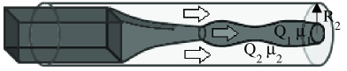
Figure 1: Microfluidic device used to perform the experiments. In inner fluid is injected at rate $Q_{1}$ through the tip of a tapered square capillary inside a cylindrical capillary in which an outer fluid is injected at rate $Q_{2}$.

Flow patterns are observed through an optical light microscope and pictures are recorded with a fast camera. They vary significantly with operational ($Q_{1}$, $Q_{2}$), geometrical ($R_{2}$), and system parameters ($\mu_{1}$, $\mu_{2}$, $\sigma$). Fluids used in this study are water at $1$ mPa$\cdot$s, mixtures of water and glycerine at $55$ and $650$ mPa$\cdot$s, silicone oil at $235$ mPa$\cdot$s and hexadecane at $3$ mPa$\cdot$s. The surface tension between the fluids are changed by adding sodium dodecyl sulfate (SDS) in aqueous solutions and Span 80 in hexadecane.

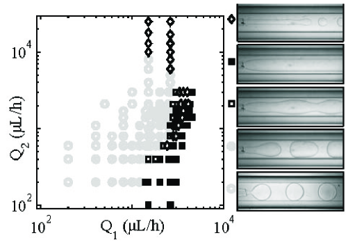
Figure 2: Map of the flow behavior in the ($Q_{1}$, $Q_{2}$) plane. The droplet regime comprises droplets smaller than the capillary $(\large{\color[rgb]{0.6,0.6,0.6}\circ}\normalsize)$ and plug-like droplets confined by this capillary $(\large{\color[rgb]{0.6,0.6,0.6}\bullet}\normalsize)$. Jets are observed in various forms: jets with visible peristaltic modulations convected downstream $(\footnotesize\square\normalsize)$, wide straight jets $(\footnotesize\blacksquare\normalsize)$ that are stable throughout the $\sim 5$ cm long channel, and thin jets breaking into droplets at a well defined location $(\footnotesize\lozenge\normalsize)$. Parameters are: $R_{2}=275~{}\mu$m, inner viscosity $\mu_{i}=55$ cP, outer viscosity $\mu_{e}=235$ cP, surface tension $\sigma=16~{}mN/m$.

Figure 2 displays the typical outcome of an experiment where the flow rates are varied for a given system (here the inner solution is a 50 $\%$ in weight glycerine in water solution with SDS for which $\mu_{1}=55$ mPa$\cdot$s and the outer one is a silicone oil for which $\mu_{2}=235$ mPa$\cdot$s). A droplet regime is found for low $Q_{1}$, with either droplets emitted periodically right at the nozzle - symbol $(\large{\color[rgb]{0.6,0.6,0.6}\circ}\normalsize)$ - or non spherical plug-like droplets resulting from the instability of an emerging oscillating jet $(\large{\color[rgb]{0.6,0.6,0.6}\bullet}\normalsize)$. Jets are found in the bottom right corner of Fig. 2 with different visual aspects: wavy jets with features that are convected downstream $(\footnotesize\square\normalsize)$ and, for larger values of $Q_{1}$, straight jets $(\footnotesize\blacksquare\normalsize)$ that persist throughout the cylindrical capillary. For large values of the external flow rate $Q_{2}$, we observe what we call jetting: thin and rather straight jets $(\footnotesize\lozenge\normalsize)$ that extend over some distance in the capillary tube before breaking into droplets at a well-defined and reproducible location. This “jet length” increases with $Q_{1}$ for a fixed value of $Q_{2}$. Similar “dynamic phase diagrams” have been reported for similar and more complex microfluidic geometries Thorsen:2001 ; Anna:2003 ; Cramer:2004 ; Tice:2004 ; Guillot:2005 ; Utada:2008 ; Dollet:2008 .

IV Results

In order to compare the numerical results with the experimental ones we have first to relate the dimensional parameters used in the experimental setup ($\it{i.e.}$ the imposed liquid flow rates $Q_{1}$ and $Q_{2}$ of the inner and outer liquids, respectively, $R_{2}$, $\sigma$ and the densities and viscosities of both liquids) with our dimensionless parameters $Re$, $We$, $R$, $\mu$ and $\rho$. To do that we need to obtain the radius of the jet, $R_{1}$, and the velocity at the interface, $U$, from the imposed flow rates and geometrical constrain. By assuming that the flow is fully developed with a velocity profile given by (1) we get:

$$R_{1}=R_{2}\left\{1+Q\left[1+(1+\mu/Q)^{1/2}\right]\right\}^{-1/2},\,\,U=\frac{2Q_{2}}{\pi R_{1}^{2}(R^{2}-1)},$$ (29)

where $Q=Q_{2}/Q_{1}$. From these expressions, for a given pair of liquids and a certain capillary, one can obtain the theoretical mapping in a $\{Q_{1},Q_{2}\}$ plane of the absolutely and convectively unstable regimes, corresponding to dripping and jetting regimes, respectively.

Figures (3) provide a comparison of (i) the approximate analytical model proposed by Guillot et al.Guillot2007 , (ii) the exact analytical model here proposed for $Re=0$, and (iii) the complete model including inertia, here numerically solved using Chebyshev collocation methods.

Figure 3: Map of the flow behavior in the ($Q_{1}$, $Q_{2}$) plane for various geometries and fluids. Gray symbols correspond to droplets regimes and black symbols to jets regimes. Lines are the transition predict by the model without adjustable parameters. The red line corresponds to the linear analysis perform using the averaged (lubrication) approximation (Guillot et al. 2007), the blue line to the exact analytical model without inertia and the blue line to the numerical one taking into account the inertia. Comparisons between experimental and theoretical transitions are in good agreement for all the experimental conditions presented here. (a1) is obtained for $R_{2}=275~{}\mu$m, $\mu_{1}=55$ mPa$\cdot$s, $\mu_{2}=235$ mPa$\cdot$s and $\sigma=24~{}mN/m$; (a2) for $R_{2}=430~{}\mu$m, $\mu_{1}=55$ mPa$\cdot$s, $\mu_{2}=235$ mPa$\cdot$s and $\sigma=24~{}mN/m$; (a3) is o btained with $R_{2}=275~{}\mu$m, $\mu_{1}=55$ mPa$\cdot$s, $\mu_{2}=235$ mPa$\cdot$s and $\sigma=16~{}mN/m$; (b1) is obtained with $R_{2}=275~{}\mu$m, $\mu_{1}=1$ mPa$\cdot$s, $\mu_{2}=3$ mPa$\cdot$s and $\sigma=12~{}mN/m$; (b2) is obtained with $R_{2}=275~{}\mu$m, $\mu_{1}=1$ mPa$\cdot$s, $\mu_{2}=3$ mPa$\cdot$s and $\sigma=0.12~{}mN/m$; (c1) is obtained with $R_{2}=275~{}\mu$m, $\mu_{1}=235$ mPa$\cdot$s, $\mu_{2}=55$ mPa$\cdot$s and $\sigma=24~{}mN/m$; (d1) is obtained with $R_{2}=275~{}\mu$m, $\mu_{1}=650$ mPa$\cdot$s, $\mu_{2}=235$ mPa$\cdot$s and $\sigma=24~{}mN/m$.

V Discussion

V.0.1 Low outer flow rate values

This region deals with the transition from the plug regime to the wavy/straight jet regime. Jets obtained in this region are highly confined by the walls. In our experimental conditions, Reynolds number is always lower than one in this region.

In all the experiments, the three models predict almost the same transition at low values of $Q_{2}$ with a very good degree of agreement. As expected, inertia does not play a major role for this range of flow rate, and the differences between the complete model with or without inertia cannot be noticed. However, the analysis obtained in the framework of the lubrication approximation gives a transition at slightly lower (higher) values of $Q_{1}$ when $\mu>$1 ($\mu<$1). Results obtained through this approximate analysis seems to be a little bit more accurate that the ones obtained with the whole model. The main difference between the lubrication approximation used to perform the linear analysis Guillot2007 , which holds for high confinement at any viscosity ratio, and the “exact” models is the former does not consider the normal viscous stresses balance at the interface, while the later ones do so. Interestingly, at the time of the experimental comparison, perturbation amplitudes may become comparable to the thickness of the outer layer at high confinement, even though they remained small compared to the jet radius; in these cases, the accuracy of exact linear models is overcome by the approximate averaged model. Informally speaking, the averaged -more “forgiving”- model seems to yield a better approximation for visible perturbation amplitudes, while the “exact” ones -more sensitive- should depart more significantly from experiments owing to non-linear effects for high confinement (finite perturbation amplitudes).

Thus, at low Reynolds number and for high value of confinement, the various analyses presented in this paper allow to predict quantitatively the transition between a droplet and jet regime. In spite of the number of approximations, the averaged model appears to be a simple and powerful tool to predict the transition in this range of low outer flow rate.

V.0.2 High outer flow rate values

This range of flow rate concerns the region where, by changing the flow rate, we can obtain a transition between a droplet and a jetting regime. Jets obtained in this region are thin and hardly affected by the walls. Note that the Reynolds number can be higher than the unity in some of our experimental conditions.

When we compare the experimental observations with the results obtained by the different models it clearly appears that the complete “exact” models provide a better prediction of the transition between the droplet and the jetting regime than the averaged model. We can also notice the effect of inertia in Fig. 3(b2) where the two lines clearly split at high values of $Q_{2}$. Unfortunately, we do not have enough experimental data to validate the fact that inertia promotes transition to dripping for smaller outer flow rates.

The averaged model fails for low degree of confinement. This is mainly due to the fact that the radial component of the velocity can not be neglected over the axial velocity and that the recirculations inside the perturbed jet have to be taken into account, as well as the normal stresses at the interface. In other words, the averaged lubrication approximation used is not valid in this case. The range of $R$ in which the approximation still holds depends on the viscosity ratio between both fluids.

When the transition towards jetting is studied, the complete model clearly gives better results and allows to predict quantitatively the transition between dripping and jetting. The effect of inertia will have to be checked experimentally to confirm the prediction of Fig. 3(b1).

VI Conclusions

In this work, we have studied the stability of confined capillary jet at low Reynolds numbers by considering the transition from a steady jet to a dripping system in terms of a convective to absolute instability transition. We propose both analytical and numerical analyses to describe extensive experimental results obtained in a cylindrical geometry. Predictions obtained in high degree of jet confinement are in very good agreement with all the analysis presented in this paper. The linear analysis proposed in Guillot2007 using the lubrication approximation seems to be a powerful and rather simple tool to predict the transition in this range of confinement. However this analysis fails for low degree of confinement and, in this latter case, it is necessary to go through a complete analysis of the flow to get a good agreement between the experimental results and the predictions. The effect of inertia has also been introduced in this work. Inertia seems to promote droplet formation at lower outer flow rates, but we do not have enough to data to confirm experimentally this prediction. Thus, further studies should be performed in this range of flow rate to confirm this effect.

The authors gratefully acknowledge support from the Aquitaine Région. They wish to thank A. Colin, A. Ajdari and M. Joanicot for valuable discussions. Partial support from the Ministry of Science and Education (Spain) through Grant No. DPI2007-63559 is acknowledged in this work.

References

- [1] S. J. Leib and M. E. Goldstein. Convective and absolute instability of a viscous liquid jet. Phys. Fluids, 29:952–954, 1986.
- [2] S. P. Lin and Z. W. Lian. Absolute instability of a liquid jet in a gas. Phys. Fluids A, 1:490–493, 1989.
- [3] C. Clanet and J. C. Lasheras. Transition from dripping to jetting. J. Fluid Mech., pages 307–326, 1999.
- [4] A. Sevilla, J. M. Gordillo, and C. Martinez-Bazan. The effect of the diameter ratio on the absolute and convective instability of free coflowing jets. Physics of Fluids, 14(9):3028–3038, 2002.
- [5] S. P. Lin. Breakup of Liquid Sheets and Jets. Cambridge University Press, 2003.
- [6] R. Suryo and O. A. Basaran. Tip streaming from a liquid drop forming from a tube in a co-flowing outer fluid. Phys. Fluids, 18:082102, 2006.
- [7] Alfonso M. Gañán-Calvo and Pascual Riesco-Chueca. Jetting-dripping transition of a liquid jet in a lower viscosity co-flowing immiscible liquid: the minimum flow rate in flow focusing. J. Fluid Mech., 553:75–84, 2006.
- [8] A. M. Gañán-Calvo. Generation of steady liquid microthreads and micron-sized monodisperse sprays in gas streams. Phys. Rev. Lett., 80:285–288, 1998.
- [9] S. L. Anna, N. Bontoux, and H. A. Stone. Formation of dispersions using ”flow focusing” in microchannels. Appl. Phys. Lett., 82:364–366, 2003.
- [10] P. Garstecki, I. Gitlin, W. Diluzio, E. Kumacheva, H. A. Stone, and G. M. Whitesides. Formation of monodisperse bubbles in a microfluidic flow-focusing device. Appl. Phys. Lett., 85:2649–2651, 2004.
- [11] M. Cloupeau and B. Prunet-Foch. Electrostatic spraying of liquids in cone-jet mode. J. Electrostatics, 22(2):135–159, 1989.
- [12] A. M. Gañán-Calvo, J. Dávila, and A. Barrero. Current and droplets size in the electrospraying of liquid. Scaling laws. J. Aerosol Sci., 28(2):249–275, 1997.
- [13] A. S. Utada, E. Lorenceau, D. R. Link, P. D. Kaplan, H. A. Stone, and D. A. Weitz. Monodisperse double emulsions generated from a microcapillary device. Science, 308:537–541, 2005.
- [14] P. Guillot, A. Colin, A. S. Utada, and A. Ajdari. Stability of a jet in confined pressure-driven biphasic flows at low reynolds number. Phys. Rev. Lett., 99:104502, 2007.
- [15] W. van Saarlos. Dynamical velocity selection: marginal stability. Phys. Rev. Lett., 58:2571–2574, 1987.
- [16] W. van Saarlos. Front propagation into unstable states: marginal stability as a dynamical mechanism for velocity selection. Phys. Rev. A, 37:211–229, 1988.
- [17] M. R. Khorrami. A chebychev spectral collocation method using a staggered grid for the stability of cylindrical flows. Int.J. Numer. Methods Fluids., 12:825, 1991.
- [18] A. M. Gañán-Calvo, M. A. Herrada, and P. Garstecki. Bubbling in unbounded coflowing liquids. Physical Review Letters, 96:124504, 2006.
- [19] T. J. Bridges and P. J. Morris. Differential eigenvalue problems in which the parameter appears nonlinearly. J. Comput. Phys., 55:437, 1984.
- [20] T. Thorsen, R. W. Roberts, F. H. Arnold, and S. R. Quake. Dynamic pattern formation in a vesicle-generating microfluidic device. Phys. Rev. Lett., 86:4163, 2001.
- [21] C. Cramer, P. Fischer, and E. J. Windhab. Drop formation in a co-flowing ambient fluid. Chemical Engineering Science, 59:3045 – 3058, 2004.
- [22] J. D. Tice, A. D. Lyon, and R. F. Ismagilov. Effects of viscosity on droplet formation and mixing in microfluidic channels. Analytica Chimica Acta, 507:73–77, 2004.
- [23] P. Guillot and A. Colin. Stability of parallel flows in a microchannel after a t junction. Phys. Rev. E, 72:066301, 2005.
- [24] A. S. Utada, A. Fernandez-Nieves, J. M. Gordillo, and D. A. Weitz. Absolute instability of a liquid jet in a coflowing stream. Phys. Rev. Lett., 100:014502, 2008.
- [25] B. Dollet, W. van Hoeve, J.-P. Raven, P. Marmottant, and M. Versluis. Role of the channel geometry on the bubble pinch-off in flow-focusing devices. Phys. Rev. Lett., 100:034504, 2008.