Regularity of Solutions to Regular Shock Reflection for Potential Flow

Abstract.

The shock reflection problem is one of the most important problems in mathematical fluid dynamics, since this problem not only arises in many important physical situations but also is fundamental for the mathematical theory of multidimensional conservation laws that is still largely incomplete. However, most of the fundamental issues for shock reflection have not been understood, including the regularity and transition of the different patterns of shock reflection configurations. Therefore, it is important to establish the regularity of solutions to shock reflection in order to understand fully the phenomena of shock reflection. On the other hand, for a regular reflection configuration, the potential flow governs the exact behavior of the solution in $C^{1,1}$ across the pseudo-sonic circle even starting from the full Euler flow, that is, both of the nonlinear systems are actually the same in an physically significant region near the pseudo-sonic circle; thus, it becomes essential to understand the optimal regularity of solutions for the potential flow across the pseudo-sonic circle (the transonic boundary from the elliptic to hyperbolic region) and at the point where the pseudo-sonic circle (the degenerate elliptic curve) meets the reflected shock (a free boundary connecting the elliptic to hyperbolic region). In this paper, we study the regularity of solutions to regular shock reflection for potential flow. In particular, we prove that the $C^{1,1}$-regularity is optimal for the solution across the pseudo-sonic circle and at the point where the pseudo-sonic circle meets the reflected shock. We also obtain the $C^{2,\alpha}$ regularity of the solution up to the pseudo-sonic circle in the pseudo-subsonic region. The problem involves two types of transonic flow: one is a continuous transition through the pseudo-sonic circle from the pseudo-supersonic region to the pseudo-subsonic region; the other a jump transition through the transonic shock as a free boundary from another pseudo-supersonic region to the pseudo-subsonic region. The techniques and ideas developed in this paper will be useful to other regularity problems for nonlinear degenerate equations involving similar difficulties.

1. Introduction

We are concerned with the regularity of global solutions to shock wave reflection by wedges. The shock reflection problem is one of the most important problems in mathematical fluid dynamics, which not only arises in many important physical situations but also is fundamental for the mathematical theory of multidimensional conservation laws that is still largely incomplete; its solutions are building blocks and asymptotic attractors of general solutions to the multidimensional Euler equations for compressible fluids (cf. Courant-Friedrichs [14], von Neumann [36], Glimm-Majda [21], and Morawetz [33]; also see [2, 8, 20, 22, 28, 34, 35]).

In Chen-Feldman [10], the first global existence theory of shock reflection configurations for potential flow has been established when the wedge angle $\theta_{w}$ is large, which converge to the unique solution of the normal reflection when $\theta_{w}$ tends to $\pi/2$. However, most of the fundamental issues for shock reflection by wedges have not been understood, including the regularity and transition of the different patterns of shock reflection configurations. Therefore, it is important to establish the regularity of solutions to shock reflection in order to understand fully the phenomena of shock reflection, including the case of potential flow which is widely used in aerodynamics (cf. [3, 13, 21, 32, 33]). On the other hand, for the regular reflection configuration as in Fig. 1, the potential flow governs the exact behavior of solutions in $C^{1,1}$ across the pseudo-sonic (sonic, for short below) circle ${P_{1}}{P_{4}}$ even starting from the full Euler flow, that is, both of the nonlinear systems are actually the same in a physically significant region near the sonic circle; thus, it becomes essential to understand the optimal regularity of solutions for the potential flow across the sonic circle ${P_{1}}{P_{4}}$ and at the point ${P_{1}}$ where the sonic circle meets the reflected shock.

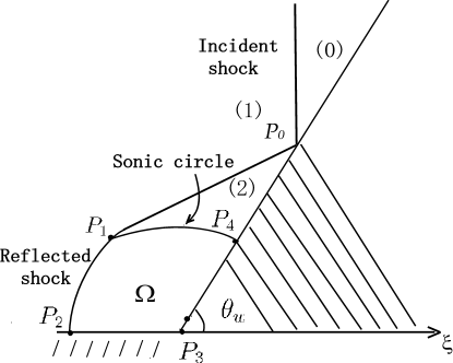
Figure 1. Regular Reflection Configuration

In this paper, we develop a mathematical approach in Sections 2–4 to establish the regularity of solutions to regular shock reflection with the configuration as in Fig. 1 for potential flow. In particular, we prove that the $C^{1,1}$-regularity is optimal for the solution across the open part ${P_{1}}{P_{4}}$ of the sonic circle (the degenerate elliptic curve) and at the point ${P_{1}}$ where the sonic circle meets the reflected shock (as a free boundary). The problem involves two types of transonic flow: one is a continuous transition through the sonic circle ${P_{1}}{P_{4}}$ from the pseudo-supersonic (supersonic, for short below) region (2) to the pseudo-subsonic (subsonic, for short below) region $\Omega$; the other is a jump transition through the transonic shock as a free boundary from the supersonic region (1) to the subsonic region $\Omega$. To achieve the optimal regularity, one of the main difficulties is that the part ${P_{1}}{P_{4}}$ of the sonic circle is the transonic boundary separating the elliptic region from the hyperbolic region. Near ${P_{1}}{P_{4}}$, the solution is governed by a nonlinear equation, whose main part has the form:

$$(2x-a\psi_{x})\psi_{xx}+b\psi_{yy}-\psi_{x}=0,$$ (1.1)

where $a,b>0$ are constants, and which is elliptic in $\{x>0\}$ where $\psi>0$, with elliptic degeneracy at $\{x=0\}$ where $\psi=0$. We analyze the features of equations modeled by (1.1) and prove the $C^{2,\alpha}$ regularity of solutions of shock reflection problem in the elliptic region up to the open part ${P_{1}}{P_{4}}$ of the sonic circle. As a corollary, we establish that the $C^{1,1}$-regularity is actually optimal across the transonic boundary ${P_{1}}{P_{4}}$ from the elliptic to hyperbolic region. Since the reflected shock ${P_{1}}{P_{2}}$ is regarded as a free boundary connecting the hyperbolic region (1) with the elliptic region $\Omega$ for the nonlinear second-order equation of mixed type, another difficulty for the optimal regularity of the solution is that the point ${P_{1}}$ is exactly the one where the degenerate elliptic curve ${P_{1}}{P_{4}}$ meets a transonic free boundary for the nonlinear partial differential equation of second order. As far as we know, this is the first optimal regularity result for solutions to a free boundary problem of nonlinear degenerate elliptic equations at the point where an elliptic degenerate curve meets the free boundary. To achieve this, we construct two sequences of points such that the corresponding sequences of values of $\psi_{xx}$ have different limits at ${P_{1}}$; this is done by employing the $C^{2,\alpha}$ regularity of the solution up to ${P_{1}}{P_{4}}$ excluding the point ${P_{1}}$, and by studying detailed features of the free boundary conditions on the free boundary ${P_{1}}{P_{2}}$, i.e., the Rankine-Hugoniot conditions.

We note that the global theory of existence and regularity of regular reflection configurations for the polytropic case $\gamma>1$, established in [10] and Sections 2–4, applies to the isothermal case $\gamma=1$ as well. The techniques and ideas developed in this paper will be useful to other regularity problems for nonlinear degenerate equations involving similar difficulties.

The regularity for certain degenerate elliptic and parabolic equations has been studied (cf. [4, 16, 30, 37, 38] and the references cited therein). The main feature that distinguishes equation (1.1) from the equations in Daskalopoulos-Hamilton [16] and Lin-Wang [30] is the crucial role of the nonlinear term $-a\psi_{x}\psi_{xx}$. Indeed, if $a=0$, then (1.1) becomes a linear equation

$$2x\psi_{xx}+b\psi_{yy}-\psi_{x}=0.$$ (1.2)

Then $\psi_{0}(x,y):=cx^{3/2}$ is a solution of (1.2), and $\psi_{0}$ with $c>0$ also satisfies the conditions:

$$\psi>0\qquad \mbox{in}\,\,\{x>0\},$$ (1.3)

$$\psi=0\qquad \mbox{on}\,\,\{x=0\},$$ (1.4)

$$\partial_{y}\psi=0\qquad\,\,\, \mbox{on}\,\,\{y=\pm 1\}.$$ (1.5)

Let $\psi$ be a solution of (1.2) in $Q_{1}:=(0,1)\times(-1,1)$ satisfying (1.3)–(1.5). Then the comparison principle implies that $\psi\geq\psi_{0}$ in $Q_{1}$ for sufficiently small $c>0$. It follows that the solutions of (1.2) satisfying (1.3)–(1.5) are not even $C^{1,1}$ up to $\{x=0\}$. On the other hand, for the nonlinear equation (1.1) with $a>0$, the function $\psi(x,y)=\frac{1}{2a}x^{2}$ is a smooth solution of (1.1) up to $\{x=0\}$ satisfying (1.3)–(1.5). More general $C^{1,1}$ solutions of (1.1) satisfying (1.3)–(1.5) and the condition

$$-Mx\leq\psi_{x}\leq\frac{2-\beta}{a}x\qquad\mbox{in}\,\,\,x>0,$$ (1.6)

with $M>0$ and $\beta\in(0,1)$, which implies the ellipticity of (1.1), can be constructed by using the methods of [10], and their $C^{2,\alpha}$ regularity up to $\{x=0\}$ follows from this paper. Another feature of the present case is that, for solutions of (1.1) satisfying (1.3)–(1.4) and (1.6), we compute explicitly $D^{2}\psi$ on $\{x=0\}$ to find that $\psi_{xx}(0,y)=\frac{1}{a}$ and $\psi_{xy}(0,y)=\psi_{yy}(0,y)=0$ for all such solutions. Thus, all the solutions are separated in $C^{2,\alpha}$ from the solution $\psi\equiv 0$, although it is easy to construct a sequence of solutions of (1.1) satisfying (1.3)–(1.4) and (1.6) which converges to $\psi\equiv 0$ in $C^{1,\alpha}$. This shows that the $C^{2,\alpha}$-regularity of (1.1) with conditions (1.3)–(1.4) and (1.6) is a truly nonlinear phenomenon of degenerate elliptic equations.

Some efforts have been also made mathematically for the shock reflection problem via simplified models, including the unsteady transonic small-disturbance (UTSD) equation (cf. Keller-Blank [26], Hunter-Keller [25], Hunter [24], Morawetz [33]) and the pressure gradient equation or the nonlinear wave system (cf. Zheng [39], Canic-Keyfitz-Kim [6]). On the other hand, in order to understand the existence and regularity of solutions near the important physical points and for the reflection problem, some asymptotic methods have been also developed (cf. Lighthill [29], Keller-Blank [26], Hunter-Keller [25], Harabetian [23], and Morawetz [33]). Also see Chen [12] for a linear approximation of shock reflection when the wedge angle is close to $\frac{\pi}{2}$ and Serre [34] for an apriori analysis of solutions of shock reflection and related discussions in the context of the Euler equations for isentropic and adiabatic fluids. We remark that our regularity results for potential flow near the sonic circle confirm rigorously the asymptotic scalings used by Hunter-Keller [25], Harabetian [23], and Morawetz [33]. Indeed, the $C^{2,\alpha}$ regularity up to the sonic circle away from ${P_{1}}$ and its proof based on the comparison with an ordinary differential equation in the radial direction confirm their asymptotic scaling via the differential equation in that region. The optimal $C^{1,1}$ regularity at ${P_{1}}$ shows that the asymptotic scaling does not work there, i.e., the angular derivatives become large, as stated in [33].

The organization of this paper is the following. In Section 2, we describe the shock reflection problem by a wedge and its solution with regular reflection configuration when the wedge angle is suitably large. In Section 3, we establish a regularity theory for solutions near the degenerate boundary with Dirichlet data for a class of nonlinear degenerate elliptic equations, in order to study the regularity of solutions to the regular reflection problem. Then we employ the regularity theory developed in Section 3 to establish the optimal regularity of solutions for $\gamma>1$ across the sonic circle ${P_{1}}{P_{4}}$ and at the point ${P_{1}}$ where the sonic circle ${P_{1}}{P_{4}}$ meets the reflected shock ${P_{1}}{P_{2}}$ in Section 4. We also established the $C^{2,\alpha}$-regularity of solutions in the subsonic region up to the sonic circle ${P_{1}}{P_{4}}$. We further observe that the existence and regularity results for regular reflection configurations for the polytropic case $\gamma>1$ apply to the isothermal case $\gamma=1$.

We remark in passing that there may exist a global regular reflection configuration when state (2) is pseudo-subsonic, which is in a very narrow regime (see [14, 36]). In this case, the regularity of the solution behind the reflected shock is direct, and the main difficulty of elliptic degeneracy does not occur. Therefore, in this paper, we focus on the difficult case for the regularity problem when state (2) is pseudo-supersonic, which will be simply called a regular shock reflection configuration, throughout this paper.

2. Shock Reflection Problem and Regular Reflection Configurations

In this section, we describe the shock reflection problem by a wedge and its solution with regular reflection configuration when the wedge angle is suitably large.

The Euler equations for potential flow consist of the conservation law of mass and the Bernoulli law for the density $\rho$ and the velocity potential $\Phi$:

$$\partial_{t}\rho+\mbox{div}_{\bf x}(\rho\nabla_{\bf x}\Phi)=0,$$ (2.1)

$$\partial_{t}\Phi+\frac{1}{2}|\nabla_{\bf x}\Phi|^{2}+i(\rho)=B_{0},$$ (2.2)

where $B_{0}$ is the Bernoulli constant determined by the incoming flow and/or boundary conditions, and

$$i^{\prime}(\rho)=p^{\prime}(\rho)/\rho=c^{2}(\rho)/\rho$$

with $c(\rho)$ being the sound speed. For polytropic gas, by scaling,

$$p(\rho)=\rho^{\gamma}/\gamma,\qquad c^{2}(\rho)=\rho^{\gamma-1},\qquad i(\rho)=\frac{\rho^{\gamma-1}-1}{\gamma-1},\qquad\gamma>1.$$ (2.3)

2.1. Shock Reflection Problem

When a plane shock in the $({\bf x},t)$–coordinates, ${\bf x}=(x_{1},x_{2})\in\mathbb{R}^{2}$, with left-state $(\rho,\nabla_{\bf x}\Phi)=(\rho_{1},u_{1},0)$ and right-state $(\rho_{0},0,0),u_{1}>0,\rho_{0}<\rho_{1}$, hits a symmetric wedge

$$W:=\{(x_{1},x_{2})\,:\,|x_{2}|<x_{1}\tan\theta_{w},x_{1}>0\}$$

head on, it experiences a reflection-diffraction process. Then the Bernoulli law (2.2) becomes

$$\partial_{t}\Phi+\frac{1}{2}|\nabla_{\bf x}\Phi|^{2}+i(\rho)=i(\rho_{0}).$$ (2.4)

This reflection problem can be formulated as the following mathematical problem.

Problem 1 (Initial-Boundary Value Problem).

Seek a solution of the system of equations (2.1) and (2.4), the initial condition at $t=0$:

$$(\rho,\Phi)|_{t=0}=\begin{cases}(\rho_{0},0)\qquad&\mbox{for}\,\,|x_{2}|>x_{1}\tan\theta_{w},x_{1}>0,\\ (\rho_{1},u_{1}x_{1})\qquad&\mbox{for}\,\,x_{1}<0,\end{cases}$$ (2.5)

and the slip boundary condition along the wedge boundary $\partial W$:

$$\nabla\Phi\cdot\nu|_{\partial W}=0,$$ (2.6)

where $\nu$ is the exterior unit normal to $\partial W$ (see Fig. 2).

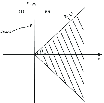
Figure 2. Initial-Boundary Value Problem

Notice that the initial-boundary value problem (2.1) and (2.4)–(2.6) is invariant under the self-similar scaling:

$$({\bf x},t)\to(\alpha{\bf x},\alpha t),\quad(\rho,\Phi)\to(\rho,\frac{\Phi}{\alpha})\qquad\quad\mbox{for}\quad\alpha\neq 0.$$

Thus, we seek self-similar solutions with the form

$$\rho({\bf x},t)=\rho(\xi,\eta),\quad\Phi({\bf x},t)=t\,\psi(\xi,\eta)\qquad\quad\mbox{for}\quad(\xi,\eta)=\frac{{\bf x}}{t}.$$

Then the pseudo-potential function $\varphi=\psi-\frac{1}{2}(\xi^{2}+\eta^{2})$ is governed by the following potential flow equation of second order:

$$\mbox{div}\,\big{(}\rho(|D\varphi|^{2},\varphi)D\varphi\big{)}+2\rho(|D\varphi|^{2},\varphi)=0$$ (2.7)

with

$$\rho(|D\varphi|^{2},\varphi)=\big{(}\rho_{0}^{\gamma-1}-(\gamma-1)(\varphi+\frac{1}{2}|D\varphi|^{2})\big{)}^{\frac{1}{\gamma-1}},$$ (2.8)

where the divergence div and gradient $D$ are with respect to the self-similar variables $(\xi,\eta)$. Then we have

$$c^{2}=c^{2}(|D\varphi|^{2},\varphi,\rho_{0}^{\gamma-1})=\rho_{0}^{\gamma-1}-(\gamma-1)(\frac{1}{2}|D\varphi|^{2}+\varphi).$$ (2.9)

Equation (2.7) is a nonlinear equation of mixed elliptic-hyperbolic type. It is elliptic if and only if

$$|D\varphi|<c(|D\varphi|^{2},\varphi,\rho_{0}^{\gamma-1}),$$ (2.10)

which is equivalent to

$$|D\varphi|<c_{*}(\varphi,\rho_{0},\gamma):=\sqrt{\frac{2}{\gamma+1}\big{(}\rho_{0}^{\gamma-1}-(\gamma-1)\varphi\big{)}}.$$ (2.11)

Shocks are discontinuities in the pseudo-velocity $D\varphi$. That is, if $\Omega^{+}$ and $\Omega^{-}:=\Omega\setminus\overline{\Omega^{+}}$ are two nonempty open subsets of $\Omega\subset\mathbb{R}^{2}$ and $S:=\partial\Omega^{+}\cap\Omega$ is a $C^{1}$–curve where $D\varphi$ has a jump, then $\varphi\in W^{1,1}_{loc}(\Omega)\cap C^{1}(\Omega^{\pm}\cup S)\cap C^{2}(\Omega^{\pm})$ is a global weak solution of (2.7) in $\Omega$ if and only if $\varphi$ is in $W^{1,\infty}_{loc}(\Omega)$ and satisfies equation (2.7) in $\Omega^{\pm}$ and the Rankine-Hugoniot condition on $S$:

$$\left[\rho(|D\varphi|^{2},\varphi)D\varphi\cdot\nu\right]_{S}=0.$$ (2.12)

The plane incident shock solution in the $({\bf x},t)$–coordinates with states $(\rho,\nabla_{\bf x}\Psi)=(\rho_{0},0,0)$ and $(\rho_{1},u_{1},0)$ corresponds to a continuous weak solution $\varphi$ of (2.7) in the self-similar coordinates $(\xi,\eta)$ with the following form:

$$\varphi_{0}(\xi,\eta)=-\frac{1}{2}(\xi^{2}+\eta^{2})\qquad\hbox{for }\,\,\xi>\xi_{0},$$ (2.13)

$$\varphi_{1}(\xi,\eta)=-\frac{1}{2}(\xi^{2}+\eta^{2})+u_{1}(\xi-\xi_{0})\qquad\hbox{for }\,\,\xi<\xi_{0},$$ (2.14)

respectively, where

$$\xi_{0}=\rho_{1}\sqrt{\frac{2(\rho_{1}^{\gamma-1}-\rho_{0}^{\gamma-1})}{(\gamma-1)(\rho_{1}^{2}-\rho_{0}^{2})}}=\frac{\rho_{1}u_{1}}{\rho_{1}-\rho_{0}}>0$$ (2.15)

is the location of the incident shock, uniquely determined by $(\rho_{0},\rho_{1},\gamma)$ through (2.12), that is, $P_{0}=(\xi_{0},\xi_{0}\tan\theta_{w})$ in Fig. 1. Since the problem is symmetric with respect to the axis $\eta=0$, it suffices to consider the problem in the half-plane $\eta>0$ outside the half-wedge

$$\Lambda:=\{\xi<0,\eta>0\}\cup\{\eta>\xi\tan\theta_{w},\,\xi>0\}.$$

Then the initial-boundary value problem (2.1) and (2.4)–(2.6) in the $({\bf x},t)$–coordinates can be formulated as the following boundary value problem in the self-similar coordinates $(\xi,\eta)$.

Problem 2.

(Boundary Value Problem) (see Fig. 1). Seek a solution $\varphi$ of equation (2.7) in the self-similar domain $\Lambda$ with the slip boundary condition on the wedge boundary $\partial\Lambda$:

$$D\varphi\cdot\nu|_{\partial\Lambda}=0$$ (2.16)

and the asymptotic boundary condition at infinity:

$$\varphi\to\bar{\varphi}:=\begin{cases}\varphi_{0}\qquad\mbox{for}\,\,\,\xi>\xi_{0},\eta>\xi\tan\theta_{w},\\ \varphi_{1}\qquad\mbox{for}\,\,\,\xi<\xi_{0},\eta>0,\end{cases}\qquad\mbox{when $\xi^{2}+\eta^{2}\to\infty$},$$ (2.17)

where (2.17) holds in the sense that $\displaystyle\lim_{R\to\infty}\|\varphi-\overline{\varphi}\|_{C(\Lambda\setminus B_{R}(0))}=0.$

2.2. Existence of Regular Reflection Configurations

Since $\varphi_{1}$ does not satisfy the slip boundary condition (2.16), the solution must differ from $\varphi_{1}$ in $\{\xi<\xi_{0}\}\cap\Lambda$ and thus a shock diffraction by the wedge occurs. In [10], the existence of global solution $\varphi$ to Problem 2 has been established when the wedge angle $\theta_{w}$ is large, and the corresponding structure of solution is as follows (see Fig. 1): The vertical line is the incident shock $S=\{\xi=\xi_{0}\}$ that hits the wedge at the point $P_{0}=(\xi_{0},\xi_{0}\tan\theta_{w})$, and state (0) and state (1) ahead of and behind $S$ are given by $\varphi_{0}$ and $\varphi_{1}$ defined in (2.13) and (2.14), respectively. The solutions $\varphi$ and $\varphi_{1}$ differ within $\{\xi<\xi_{0}\}$ only in the domain $P_{0}{P_{1}}{P_{2}}{P_{3}}$ because of shock diffraction by the wedge vertex, where the curve $P_{0}{P_{1}}{P_{2}}$ is the reflected shock with the straight segment $P_{0}{P_{1}}$. State (2) behind $P_{0}{P_{1}}$ is of the form:

$$\varphi_{2}(\xi,\eta)=-\frac{1}{2}(\xi^{2}+\eta^{2})+u_{2}(\xi-\xi_{0})+(\eta-\xi_{0}\tan\theta_{w})u_{2}\tan\theta_{w},$$ (2.18)

which satisfies

$$D\varphi\cdot\nu=0\qquad\hbox{on }\,\partial\Lambda\cap\{\xi>0\};$$

the constant velocity $u_{2}$ and the angle between $P_{0}{P_{1}}$ and the $\xi$–axis are determined by $(\theta_{w},\rho_{0},\rho_{1},\gamma)$ from the two algebraic equations expressing (2.12) and the continuous matching of $\varphi_{1}$ and $\varphi_{2}$ across $P_{0}{P_{1}}$. Moreover, the constant density $\rho_{2}$ of state (2) satisfies $\rho_{2}>\rho_{1}$, and state (2) is supersonic at the point $P_{0}$. The solution $\varphi$ is subsonic within the sonic circle for state (2) with center $(u_{2},u_{2}\tan\theta_{w})$ and radius $c_{2}=\rho_{2}^{(\gamma-1)/2}>0$ (the sonic speed of state (2)), and $\varphi$ is supersonic outside this circle containing the arc ${P_{1}}{P_{4}}$ in Fig. 1, so that $\varphi_{2}$ is the unique solution in the domain $P_{0}{P_{1}}{P_{4}}$, as argued in [8, 34]. Then $\varphi$ differs from $\varphi_{2}$ in the domain $\Omega={P_{1}}{P_{2}}{P_{3}}{P_{4}}$, where the equation is elliptic.

Introduce the polar coordinates $(r,\theta)$ with respect to the center $(u_{2},u_{2}\tan\theta_{w})$ of the sonic circle of state (2), that is,

$$\xi-u_{2}=r\cos{\theta},\quad\eta-u_{2}\tan\theta_{w}=r\sin{\theta}.$$ (2.19)

Then, for $\varepsilon\in(0,c_{2})$, we denote by $\Omega_{\varepsilon}:=\Omega\cap\{(r,\theta)\;:\;0<c_{2}-r<\varepsilon\}$ the $\varepsilon$-neighborhood of the sonic circle ${P_{1}}{P_{4}}$ within $\Omega$. In $\Omega_{\varepsilon}$, we introduce the coordinates:

$$x=c_{2}-r,\quad y=\theta-\theta_{w}.$$ (2.20)

This implies that $\Omega_{\varepsilon}\subset\{0<x<\varepsilon,\;y>0\}$ and ${P_{1}}{P_{4}}\subset\{x=0\;y>0\}$. Also we introduce the following notation for various parts of $\partial\Omega$:

$$\Gamma_{sonic}:=\partial\Omega\cap\partial B_{c_{2}}((u_{2},u_{2}\tan\theta_{w}))\equiv{P_{1}}{P_{4}};$$

$$\Gamma_{shock}:={P_{1}}{P_{2}};$$

$$\Gamma_{wedge}:=\partial\Omega\cap\partial\Lambda\equiv{P_{3}}{P_{4}}.$$

Then the global theory established in [10] indicates that there exist $\theta_{c}=\theta_{c}(\rho_{0},\rho_{1},\gamma)\in(0,\frac{\pi}{2})$ and $\alpha=\alpha(\rho_{0},\rho_{1},\gamma)\in(0,1)$ such that, when $\theta_{w}\in[\theta_{c},\frac{\pi}{2})$, there exists a global self-similar solution:

$$\Phi({\bf x},t)=t\,\varphi(\frac{\bf x}{t})+\frac{|\bf x|^{2}}{2t}\qquad\mbox{for}\,\,\frac{\bf x}{t}\in\Lambda,\,t>0,$$

with

$$\rho({\bf x},t)=\big{(}\rho_{0}^{\gamma-1}-(\gamma-1)(\Phi_{t}+\frac{1}{2}|\nabla_{\bf x}\Phi|^{2})\big{)}^{\frac{1}{\gamma-1}}$$

of Problem 1 (equivalently, Problem 2) for shock reflection by the wedge, which satisfies that, for $(\xi,\eta)=\frac{{\bf x}}{t}$,

$$\begin{split}&\varphi\in C^{0,1}(\Lambda),\\ &\varphi\in C^{\infty}(\Omega)\cap C^{1,\alpha}(\bar{\Omega}),\\ &\varphi=\left\{\begin{array}[]{ll}\varphi_{0}\qquad\mbox{for}\,\,\xi>\xi_{0}\mbox{ and }\eta>\xi\tan\theta_{w},\\ \varphi_{1}\qquad\mbox{for}\,\,\xi<\xi_{0}\mbox{ and above the reflection shock}\,\,P_{0}{P_{1}}{P_{2}},\\ \varphi_{2}\qquad\mbox{in}\,\,P_{0}{P_{1}}{P_{4}}.\end{array}\right.\end{split}$$ (2.21)

Moreover,

1. equation (2.7) is elliptic in $\Omega$;

2. $\varphi\geq\varphi_{2}\qquad\text{in}\;\;\Omega$;

3. the reflected shock $P_{0}{P_{1}}{P_{2}}$ is $C^{2}$ at ${P_{1}}$ and $C^{\infty}$ except ${P_{1}}$;

4. there exists $\varepsilon_{0}\in(0,\;\frac{c_{2}}{2})$ such that $\varphi\in C^{1,1}(\overline{\Omega_{\varepsilon_{0}}})\cap C^{2}(\overline{\Omega_{\varepsilon_{0}}}\setminus\overline{\Gamma}_{sonic})$; moreover, in the coordinates (2.20),

   $$\|\varphi-\varphi_{2}\|^{(par)}_{2,0,\Omega_{\varepsilon_{0}}}\!:=\!\sum_{0\leq k+l\leq 2}\sup_{z\in\Omega_{\varepsilon_{0}}}(x^{k+\frac{l}{2}-2}|\partial_{x}^{k}\partial_{y}^{l}(\varphi-\varphi_{2})(x,y)|)<\infty;$$ (2.22)

5. there exists $\delta_{0}>0$ so that, in the coordinates (2.20),

   $$|\partial_{x}(\varphi-\varphi_{2})(x,y)|\leq\frac{2-\delta_{0}}{\gamma+1}x\qquad\;\text{in}\;\;\Omega_{\varepsilon_{0}};$$ (2.23)

6. there exist $\omega>0$ and a function $y=\hat{f}(x)$ such that, in the coordinates (2.20),

   $$\begin{split}&\Omega_{\varepsilon_{0}}=\{(x,y)\,:\,x\in(0,\;\varepsilon_{0}),\;\;0<y<\hat{f}(x)\},\\ &\Gamma_{shock}\cap\{0\leq x\leq\varepsilon_{0}\}=\{(x,y):x\in(0,\;\varepsilon_{0}),\;\;y=\hat{f}(x)\},\end{split}$$ (2.24)

   and

   $$\|\hat{f}\|_{C^{1,1}([0,\;\varepsilon_{0}])}<\infty\;\;,\;\;\frac{d\hat{f}}{dx}\!\geq\omega>0\!\;\;\;\text{for}\;\;0<x<\varepsilon_{0}.$$ (2.25)

The existence of state (2) of the form (2.18) with constant velocity $(u_{2},u_{2}\tan\theta_{w})$, $u_{2}>0$, and constant density $\rho_{2}>\rho_{1}$, satisfying (2.12) and $\varphi_{1}=\varphi_{2}$ on $P_{0}{P_{1}}$, is shown in [10, Section 3] for $\theta_{w}\in[\theta_{c},\frac{\pi}{2})$. The existence of a solution $\varphi$ of Problem 2, satisfying (2.21) and property (iv) follows from [10, Main Theorem]. Property (i) follows from Lemma 5.2 and Proposition 7.1 in [10]. Property (ii) follows from Proposition 7.1 and Section 9 in [10], which assert that $\varphi-\varphi_{2}\in\mathcal{K}$, where the set $\mathcal{K}$ defined by (5.15) in [10], which implies property (ii). Property (v) follows from Propositions 8.1–8.2 and Section 9 in [10]. Property (vi) follows from (5.7) and (5.25)–(5.27) in [10] and the fact that $\varphi-\varphi_{2}\in\mathcal{K}$.

These results have been extended in [11] to other wedge-angle cases.

3. Regularity near the degenerate boundary for nonlinear degenerate elliptic equations of second order

In order to study the regularity of solutions to the regular reflection problem, in this section we first study the regularity of solutions near a degenerate boundary for a class of nonlinear degenerate elliptic equations of second order.

We adopt the following definitions for ellipticity and uniform ellipticity: Let $\Omega\subset\mathbb{R}^{2}$ be open, $u\in C^{2}(\Omega)$, and

$${\mathcal{L}}u=\sum_{i,j=1}^{2}A_{ij}(x,Du)u_{ij}+B(x,Du),$$ (3.1)

where $A_{ij}(x,p)$ and $B(x,p)$ are continuous on $\overline{\Omega}\times\mathbb{R}^{2}$. The operator ${\mathcal{L}}$ is elliptic with respect to $u$ in $\Omega$ if the coefficient matrix

$$A(x,Du(x)):=[A_{ij}(x,Du(x))]$$

is positive for every $x\in\Omega$. Furthermore, ${\mathcal{L}}$ is uniformly elliptic with respect to $u$ in $\Omega$ if

$$\lambda I\leq A(x,Du(x))\leq\Lambda I\qquad\mbox{for every $x\in\Omega$},$$

where $\Lambda\geq\lambda>0$ are constants and $I$ is the $2\times 2$ identity matrix.

The following standard comparison principle for the operator ${\mathcal{L}}$ follows from [19, Theorem 10.1].

Lemma 3.1.

Let $\Omega\subset\mathbb{R}^{2}$ be an open bounded set. Let $u,v\in C(\overline{\Omega})\cap C^{2}(\Omega)$ such that the operator ${\mathcal{L}}$ is elliptic in $\Omega$ with respect to either $u$ or $v$. Let ${\mathcal{L}}u\leq{\mathcal{L}}v$ in $\Omega$ and $u\geq v$ on $\partial\Omega$. Then $u\geq v$ in $\Omega$.

3.1. Nonlinear Degenerate Elliptic Equations and Regularity Theorem

We now study the regularity of positive solutions near the degenerate boundary with Dirichlet data for the class of nonlinear degenerate elliptic equations of the form:

$${\mathcal{L}}_{1}\psi:=(2x-a\psi_{x}+O_{1})\psi_{xx}+O_{2}\psi_{xy}+(b+O_{3})\psi_{yy}-(1+O_{4})\psi_{x}+O_{5}\psi_{y}=0\quad\text{in}\;Q^{+}_{r,R},$$ (3.2)

$$\psi>0\qquad\quad\text{in}\;Q^{+}_{r,R},$$ (3.3)

$$\psi=0\qquad\quad\text{on}\;\partial Q^{+}_{r,R}\cap\{x=0\},$$ (3.4)

where $a,b>0$ are constants and, for $r,R>0$,

$$Q^{+}_{r,R}:=\{(x,y)\;:\;x\in(0,r),\;|y|<R\}\subset\mathbb{R}^{2},$$ (3.5)

and the terms $O_{i}(x,y),i=1,\dots,5$ are continuously differentiable and

$$\frac{|O_{1}(x,y)|}{x^{2}},\;\frac{|O_{k}(x,y)|}{x}\leq N\qquad\quad \text{for}\,\;k=2,\dots,5,$$ (3.6)

$$\frac{|DO_{1}(x,y)|}{x},\;|DO_{k}(x,y)|\leq N\qquad\quad \text{for}\;\;k=2,\dots,5,$$ (3.7)

in $\{x>0\}$ for some constant $N$.

Conditions (3.6)–(3.7) imply that the terms $O_{i},i=1,\cdots,5$, are “small”; the precise meaning of which can be seen in Section 4 for the shock reflection problem below (also see the estimates in [10]). Thus, the main terms of equation (3.2) form the following equation:

$$(2x-a\psi_{x})\psi_{xx}+b\psi_{yy}-\psi_{x}=0\qquad\quad\text{in}\;Q^{+}_{r,R}.$$ (3.8)

Equation (3.8) is elliptic with respect to $\psi$ in $\{x>0\}$ if $\psi_{x}<\frac{2x}{a}$. In this paper, we consider the solutions that satisfy

$$-Mx\leq\psi_{x}\leq{2-\beta\over a}x\qquad\quad\text{in}\;Q^{+}_{r,R}$$ (3.9)

for some constants $M\geq 0$ and $\beta\in(0,1)$. Then (3.8) is uniformly elliptic in every subdomain $\{x>\delta\}$ with $\delta>0$. The same is true for equation (3.2) in $Q^{+}_{r,R}$ if $r$ is sufficiently small.

Remark 3.1.

If $\hat{r}$ is sufficiently small, depending only on $a,b$, and $N$, then (3.6)–(3.7) and (3.9) imply that equation (3.2) is uniformly elliptic with respect to $\psi$ in $Q^{+}_{\hat{r},R}\cap\{x>\delta\}$ for any $\delta\in(0,\frac{\hat{r}}{2})$. We will always assume such a choice of $\hat{r}$ hereafter.

Let $\psi\in C^{2}(Q^{+}_{\hat{r},R})$ be a solution of (3.2) satisfying (3.9). Remark 3.1 implies that the interior regularity

$$\psi\in C^{2,\alpha}(Q^{+}_{\hat{r},R})\qquad\mbox{for all }\;\alpha\in(0,1)$$ (3.10)

follows first from the linear elliptic theory in two-dimensions (cf. [19, Chapter 12]) to conclude the solution in $C^{1,\alpha}$ which leads that the coefficient becomes $C^{\alpha}$ and then from the Schauder theory to get the $C^{2,\alpha}$ estimate (cf. [19, Chapter 6]), where we use the fact $O_{i}\in C^{1}(\{x>0\})$. Therefore, we focus on the regularity of $\psi$ near the boundary $\{x=0\}\cap\partial Q^{+}_{\hat{r},R}$ where the ellipticity of (3.2) degenerates.

Theorem 3.1 (Regularity Theorem).

Let $a,b,M,N,R>0$ and $\beta\in(0,\frac{1}{4})$ be constants. Let $\psi\in C(\overline{Q^{+}_{\hat{r},R}})\cap C^{2}(Q^{+}_{\hat{r},R})$ satisfy (3.3)–(3.4), (3.9), and equation (3.2) in $Q^{+}_{\hat{r},R}$ with $O_{i}=O_{i}(x,y)$ satisfying $O_{i}\in C^{1}(\overline{Q^{+}_{\hat{r},R}})$ and (3.6)–(3.7). Then

$$\psi\in C^{2,\alpha}(\overline{Q^{+}_{\hat{r}/2,{R}/{2}}})\qquad\mbox{for any}\,\,\alpha\in(0,1),$$

with

$$\psi_{xx}(0,y)=\frac{1}{a},\quad\psi_{xy}(0,y)=\psi_{yy}(0,y)=0\qquad\mbox{for all\,\, $|y|<\frac{R}{2}$}.$$

To prove Theorem 3.1, it suffices to show that, for any given $\alpha\in(0,1)$,

$$\psi\in C^{2,\alpha}(\overline{Q^{+}_{r,R/2}})\qquad\;\text{for some}\;r\in(0,\;\hat{r}/2),$$ (3.11)

since $\psi$ belongs to $C^{2,\alpha}(\overline{Q^{+}_{\hat{r}/2,R/2}\cap\{x>r/2\}})$ by (3.10).

Note that, by (3.3)–(3.4) and (3.9), it follows that

$$0<\psi(x,y)\leq{2-\beta\over 2a}x^{2}\qquad\mbox{for all }\;(x,y)\in Q^{+}_{\hat{r},R}.$$ (3.12)

The essential part of the proof of Theorem 3.1 is to show that, if a solution $\psi$ satisfies (3.12), then, for any given $\alpha\in(0,\;1)$, there exists $r\in(0,\hat{r}/2]$ such that

$$|\psi(x,y)-{1\over 2a}x^{2}|\leq Cx^{2+\alpha}\qquad\mbox{for all }\;(x,y)\in Q^{+}_{r,7R/8}.$$ (3.13)

Notice that, although $\psi^{(0)}\equiv 0$ is a solution of (3.2), it satisfies neither (3.13) nor the conclusion $\psi^{(0)}_{xx}(0,y)=\frac{1}{a}$ of Theorem 3.1. Thus it is necessary to improve first the lower bound of $\psi$ in (3.12) to separate our solution from the trivial solution $\psi^{(0)}\equiv 0$.

3.2. Quadratic Lower Bound of $\psi$

By Remark 3.1, equation (3.2) is uniformly elliptic with respect to $\psi$ inside $Q^{+}_{\hat{r},R}$. Thus, our idea is to construct a positive subsolution of (3.2), which provides our desired lower bound of $\psi$.

Proposition 3.1.

Let $\psi$ satisfy the assumptions in Theorem 3.1. Then there exist $r\in(0,\hat{r}/2]$ and $\mu>0$, depending only on $a,b,N,R,\hat{r},\beta$, and $\inf_{Q^{+}_{\hat{r},R}\cap\{x>{\hat{r}}/{2}\}}\psi$, such that

$$\psi(x,y)\geq\mu x^{2}\;\qquad\;\text{on}\;\;Q^{+}_{r,{15R}/{16}}.$$

Proof.

In this proof, all the constants below depend only on the data, i.e., $a,b,M,N,R,\hat{r},\beta$, and $\inf_{Q^{+}_{\hat{r},R}\cap\{x>{\hat{r}}/{2}\}}\psi$, unless otherwise is stated.

Fix $y_{0}$ with $|y_{0}|\leq\frac{15R}{16}$. We now prove that

$$\psi(x,y_{0})\geq\mu x^{2}\;\;\qquad\text{for}\;\;x\in(0,r).$$ (3.14)

We first note that, without loss of generality, we may assume that $R=2$ and $y_{0}=0$. Otherwise, we set $\tilde{\psi}(x,y):=\psi(x,y_{0}+\frac{R}{32}y)$ for all $(x,y)\in Q^{+}_{\hat{r},2}$. Then $\tilde{\psi}\in C(\overline{Q^{+}_{\hat{r},2}})\cap C^{2}(Q^{+}_{\hat{r},2})$ satisfies equation (3.2) with (3.6) and conditions (3.3)–(3.4) and (3.9) in $Q^{+}_{\hat{r},2}$, with some modified constants $a,b,N,\beta$ and functions $O_{i}$, depending only on the corresponding quantities in the original equation and on $R$. Moreover, $\inf_{Q^{+}_{\hat{r},2}\cap\{x>{\hat{r}}/{2}\}}\tilde{\psi}=\inf_{Q^{+}_{\hat{r},R}\cap\{x>{\hat{r}}/{2}\}}\psi$. Then (3.14) for $\psi$ follows from (3.14) for $\tilde{\psi}$ with $y_{0}=0$ and $R=2$. Thus we will keep the original notation with $y_{0}=0$ and $R=2$. Then it suffices to prove

$$\psi(x,0)\geq\mu x^{2}\;\;\qquad\text{for}\;\;x\in(0,r).$$ (3.15)

By Remark 3.1 and the Harnack inequality, we conclude that, for any $r\in(0,\hat{r}/2)$, there exists $\sigma=\sigma(r)>0$ depending only on $r$ and the data $a,b,N,R,\hat{r},\beta$, and $\inf_{Q^{+}_{\hat{r},R}\cap\{x>{\hat{r}}/{2}\}}\psi$, such that

$$\psi\geq\sigma\quad\qquad\text{on }\;Q^{+}_{\hat{r},{3}/{2}}\cap\{x>r\}.$$ (3.16)

Let $r\in(0,\hat{r}/2)$, $k>0$, and

$$0<\mu\leq\frac{\sigma(r)}{r^{2}}$$ (3.17)

to be chosen. Set

$$w(x,y):=\mu x^{2}(1-y^{2})-kxy^{2}.$$ (3.18)

Then, using (3.16)–(3.17), we obtain that, for all $x\in(0,r)$ and $|y|<1$,

$$\begin{cases}w(0,y)=0\leq\psi(0,y),\\ w(r,y)\leq\mu r^{2}\leq\psi(r,y),&\\ w(x,\pm 1)=-kx\leq 0\leq\psi(x,\pm 1).\end{cases}$$

Therefore, we have

$$w\leq\psi\;\qquad\text{on}\;\partial Q^{+}_{r,1}.$$ (3.19)

Next, we show that $w$ is a strict subsolution ${\mathcal{L}}_{1}w>0$ in $Q^{+}_{r,1}$, if the parameters are chosen appropriately. In order to estimate ${\mathcal{L}}_{1}w$, we denote

$$A_{0}:=\frac{k}{\mu}$$ (3.20)

and notice that

$$w_{yy}=-2x(\mu x+k)=-2x(\mu x+k)\big{(}(1-y^{2})+y^{2}\big{)}=-2\mu x(1-y^{2})(x+A_{0})-2ky^{2}x(\frac{x}{A_{0}}+1).$$

Then, by a direct calculation and simplification, we obtain

$${\mathcal{L}}_{1}w=2\mu x(1\!-\!y^{2})I_{1}+ky^{2}I_{2},$$ (3.21)

where

$$I_{1}=1\!-\!2\mu a(1\!-\!y^{2}\!)\!-\!O_{4}\!+\!\frac{O_{1}}{x}\!-\!\big{(}(b\!+\!O_{3})-yO_{5}\big{)}(x\!+\!A_{0})\!-\!\frac{y(2x\!+\!A_{0})}{x}O_{2},$$

$$I_{2}=(1\!+\!O_{4})\!+\!2\mu a(1\!-\!y^{2})\!-\!2(b\!+\!O_{3})x(\frac{x}{A_{0}}\!+\!1)\!-\!2yx(\frac{x}{A_{0}}\!+\!1)O_{5}\!-\!2y(\frac{2x}{A_{0}}\!+\!1)O_{2}.$$

Now we choose $r$ and $\mu$ so that ${\mathcal{L}}_{1}w\geq 0$ holds. Clearly, ${\mathcal{L}}_{1}w\geq 0$ if $I_{1},I_{2}\geq 0$. By (3.6), we find that, in $Q^{+}_{r,1}$,

$$\begin{split}&I_{1}\geq 1-2\mu a-C_{0}r-(b+N+C_{0}r)A_{0},\\ &I_{2}\geq 1-C_{0}r-\frac{r}{A_{0}}C_{0}r.\end{split}$$ (3.22)

Choose $r_{0}$ to satisfy the smallness assumptions stated above and

$$0<r_{0}\leq\min\{\frac{1}{4C_{0}},\frac{b+N}{C_{0}},\frac{1}{8\sqrt{C_{0}(b+N)}},\frac{\hat{r}}{2}\},$$ (3.23)

where $C_{0}$ is the constant in (3.22). For such a fixed $r_{0}$, we choose $\mu_{0}$ to satisfy (3.17) and

$$\mu_{0}\leq\frac{1}{8a},$$ (3.24)

and $A_{0}$ to satisfy

$$4C_{0}r_{0}^{2}<A_{0}<\frac{1}{8(b+N)},$$ (3.25)

where we have used (3.23) to see that $4C_{0}r_{0}^{2}<\frac{1}{8(b+N)}$ in (3.25). Then $k$ is defined from (3.20). From (3.22)–(3.25),

$$I_{1},\;I_{2}>0,$$

which implies that

$${\mathcal{L}}_{1}w>0\qquad\text{in }\;Q^{+}_{r,1}$$ (3.26)

whenever $r\in(0,\;r_{0}]$ and $\mu\in(0,\;\mu_{0}]$.

By (3.19), (3.26), Remark 3.1, and the comparison principle (Lemma 3.1), we have

$$\psi(x,y)\geq w(x,y)=\mu x^{2}(1-y^{2})-kxy^{2}\;\qquad\text{in}\;\;Q^{+}_{r,1}.$$

In particular,

$$\psi(x,0)\geq\mu x^{2}\;\qquad\text{for}\;\;x\in[0,\;r].$$ (3.27)

This implies (3.15), thus (3.14). The proof is completed. ∎

With Proposition 3.1, we now make the $C^{2,\alpha}$ estimate of $\psi$.

3.3. ${\boldsymbol{C}^{2,\alpha}}$ Estimate of ${\boldsymbol{\psi}}$

If $\psi$ satisfies (3.2)–(3.4) and (3.9), it is expected that $\psi$ is “very close” to $\frac{x^{2}}{2a}$, which is a solution to (3.8). More precisely, we now prove (3.13). To achieve this, we study the function

$$W(x,y):=\frac{x^{2}}{2a}-\psi(x,y).$$ (3.28)

By (3.2), $W$ satisfies

$$\begin{split}&{\mathcal{L}}_{2}W:=\!(x\!+\!aW_{x}\!+\!O_{1})W_{xx}\!\!+\!O_{2}W_{xy}\!\\ &\phantom{aaaaa}\,\,\,\,\,+\!(b\!+\!O_{3})W_{yy}\!-\!(2\!+\!O_{4})W_{x}\!+\!O_{5}W_{y}\!\!=\frac{O_{1}-xO_{4}}{a}\qquad\text{in}\;Q^{+}_{\hat{r},R},\end{split}$$ (3.29)

$$W(0,y)=0\qquad\qquad\qquad\qquad\qquad\qquad\qquad\text{on}\;\partial Q^{+}_{\hat{r},R}\cap\{x=0\},$$ (3.30)

$$-{1-\beta\over a}x\leq W_{x}(x,y)\leq(M+{1\over a})x\qquad\qquad\text{in}\;Q^{+}_{\hat{r},R}.$$ (3.31)

Lemma 3.2.

Let $a,b,N,R,\hat{r},\beta$, and $O_{i}$ be as in Theorem 3.1. Let $\mu$ be the constant determined in Proposition 3.1. Then there exist $\alpha_{1}\in(0,\;1)$ and $r_{1}>0$ such that, if $W\in C(\overline{Q^{+}_{\hat{r},R}})\cap C^{2}(Q^{+}_{\hat{r},R})$ satisfies (3.29)–(3.31), then

$$W(x,y)\leq\frac{1-\mu_{1}}{2ar^{\alpha}}x^{2+\alpha}\;\;\qquad\text{in}\;\;Q^{+}_{r,7R/8},$$ (3.32)

whenever $\alpha\in(0,\;\alpha_{1}]$ and $r\in(0,r_{1}]$ with $\mu_{1}:=\min(2a\mu,1/2)$.

Proof.

In the proof below, all the constants depend only on the data, i.e., $a,b,N,\beta,R,\hat{r}$, $\inf_{Q^{+}_{\hat{r},R}\cap\{x>{\hat{r}}/{2}\}}\psi$, unless otherwise is stated.

By Proposition 3.1,

$$W(x,y)\leq\frac{1-\mu_{1}}{2a}x^{2}\qquad\quad\mbox{in $Q^{+}_{r_{0},15R/16}$},$$ (3.33)

where $r_{0}$ depend only on $a,b,N,R,\hat{r}$, and $\beta$.

Fix $y_{0}$ with $|y_{0}|\leq\frac{7R}{8}$. We now prove that

$$W(x,y_{0})\leq\frac{1-\mu_{1}}{2ar^{\alpha}}x^{2+\alpha}\;\;\qquad\text{for}\;\;x\in(0,r).$$

By a scaling argument similar to the one in the beginning of proof of Lemma 3.1, i.e., considering the function $\tilde{\psi}(x,y)=\psi(x,y_{0}+\frac{R}{32}y)$ in $Q^{+}_{\hat{r},2}$, we conclude that, without loss of generality, we can assume that $y_{0}=0$ and $R=2$. That is, it suffices to prove that

$$W(x,0)\leq\frac{1-\mu_{1}}{2ar^{\alpha}}x^{2+\alpha}\;\;\qquad\text{for}\;\;x\in(0,r)$$ (3.34)

for some $r\in(0,r_{0}),\alpha\in(0,\alpha_{1})$, under the assumptions that (3.29)–(3.31) hold in $Q^{+}_{\hat{r},2}$ and (3.33) holds in $Q^{+}_{r_{0},2}$.

For any given $r\in(0,r_{0})$, let

$$A_{1}r^{\alpha}=\frac{1-\mu_{1}}{2a},\quad B_{1}=\frac{1-\mu_{1}}{2a},$$ (3.35)

$$v(x,y)=A_{1}x^{2+\alpha}(1-y^{2})+B_{1}x^{2}y^{2}.$$ (3.36)

Since (3.30) holds on $\partial Q^{+}_{\hat{r},2}\cap\{x=0\}$ and (3.33) holds in $Q^{+}_{r_{0},2}$, then, for all $x\in(0,r)$ and $|y|\leq 1$, we obtain

$$\begin{cases}v(0,y)=0=W(0,y),\\ v(r,y)=\big{(}A_{1}r^{\alpha}(1-y^{2})+B_{1}y^{2}\big{)}r^{2}=\frac{1-\mu_{1}}{2a}r^{2}\geq W(r,y),\\ v(x,\pm 1)=B_{1}x^{2}=\frac{1-\mu_{1}}{2a}x^{2}\geq W(x,\pm 1).\end{cases}$$

Thus,

$$W\leq v\;\qquad\text{on}\;\partial Q^{+}_{r,1}.$$ (3.37)

We now show that ${\mathcal{L}}_{2}v<{\mathcal{L}}_{2}W\;\;\text{in}\;Q^{+}_{r,1}.$ From (3.29),

$${\mathcal{L}}_{2}v-{\mathcal{L}}_{2}W={\mathcal{L}}_{2}v-\frac{O_{1}-xO_{4}}{a}.$$

In order to rewrite the right-hand side in a convenient form, we write the term $v_{yy}$ in the expression of ${\mathcal{L}}_{2}v$ as $(1-y^{2})v_{yy}+y^{2}v_{yy}$ and use similar expressions for the terms $v_{xy}$ and $v_{y}$. Then a direct calculation yields

$${\mathcal{L}}_{2}v-\frac{O_{1}-xO_{4}}{a}=(2+\alpha)A_{1}x^{1+\alpha}(1-y^{2})J_{1}+2B_{1}xy^{2}J_{2},$$

where

$$J_{1}=(1+\alpha)\Big{(}1+a\big{(}(2+\alpha)A_{1}x^{\alpha}(1-y^{2})+2B_{1}y^{2}\big{)}+\frac{O_{1}}{x}\Big{)}-(2+O_{4})+T_{1},$$

$$J_{2}=1+a\big{(}(2+\alpha)A_{1}x^{\alpha}(1-y^{2})+2B_{1}y^{2}\big{)}+\frac{O_{1}}{x}-(2+O_{4})+T_{2},$$

$$T_{1}=\frac{1}{(2+\alpha)A_{1}x^{1+\alpha}}\Big{(}2O_{2}xy(2B_{1}-(2+\alpha)A_{1}x^{\alpha})+2x^{2}(B_{1}-A_{1}x^{\alpha})\big{(}(b+O_{3})+O_{5}y\big{)}$$

$$\qquad\qquad\qquad\qquad\qquad-\frac{O_{1}-xO_{4}}{a}\Big{)},$$

$$T_{2}=\frac{(2+\alpha)A_{1}x^{1+\alpha}}{2B_{1}x}T_{1}.$$

Thus, in $Q^{+}_{r,1}$,

$${\mathcal{L}}_{2}v-{\mathcal{L}}_{2}W<0\quad\qquad\text{if}\,\,J_{1},\;J_{2}<0.$$ (3.38)

By (3.6) and (3.35), we obtain

$$|T_{1}|,\,|T_{2}|\leq Cr^{1-\alpha}\qquad\,\,\mbox{in $Q^{+}_{r,1}$},$$

so that, in $Q^{+}_{r,1}$,

$$J_{1}\leq(1+\alpha)\big{(}1+\frac{2+\alpha}{2}(1-\mu_{1})\big{)}-2+Cr^{1-\alpha},$$ (3.39)

$$J_{2}\leq 1+\frac{2+\alpha}{2}(1-\mu_{1})-2+Cr^{1-\alpha}.$$ (3.40)

Choose $\alpha_{1}>0$, depending only on $\mu_{1}$, so that, if $0<\alpha\leq\alpha_{1}$,

$$(1+\alpha)\Big{(}1+\frac{2+\alpha}{2}(1-\mu_{1})\Big{)}-2\leq-\frac{\mu_{1}}{4}.$$ (3.41)

Such a choice of $\alpha_{1}>0$ is possible because we have the strict inequality in (3.41) when $\alpha=0$, and the left-hand side is an increasing function of $\alpha>0$ (where we have used $0<\mu_{1}\leq 1/2$ by reducing $\mu$ if necessary). Now, choosing $r_{1}>0$ so that

$$r_{1}<\min\big{\{}\left(\frac{\mu_{1}}{4C}\right)^{\frac{1}{1-\alpha}},\;r_{0}\big{\}}$$ (3.42)

is satisfied, we use (3.39)–(3.41) to obtain

$$J_{1},J_{2}<0\quad\qquad\text{in }\;Q^{+}_{r,1}.$$

Then, by $(\ref{f})$, we obtain

$${\mathcal{L}}_{2}v<{\mathcal{L}}_{2}W\;\;\qquad\text{in}\;\;Q^{+}_{r,1}$$ (3.43)

whenever $r\in(0,\;r_{1}]$ and $\alpha\in(0,\;\alpha_{1}]$. By (3.37), (3.43), Remark 3.1, and the standard comparison principle (Lemma 3.1), we obtain

$$W\leq v\quad\qquad\text{in }\;Q^{+}_{r,1}.$$ (3.44)

In particular, using (3.35)–(3.36) with $y=0$, we arrive at (3.34). ∎

Using Lemma 3.2, we now generalize the result (3.32) for any $\alpha\in(0,1)$.

Proposition 3.2.

Let $a,b,N,R,\hat{r},\beta$, and $O_{i}$ be as in Theorem 3.1. Then, for any $\alpha\in(0,1)$, there exist positive constants $r$ and $A$ which depend only on $a,b,N,R,\hat{r},\beta$, and $\alpha$ so that, if $W\in C(\overline{Q^{+}_{\hat{r},R}})\cap C^{2}(Q^{+}_{\hat{r},R})$ satisfies (3.29)–(3.31), then

$$W(x,y)\leq Ax^{2+\alpha}\qquad\;\text{in}\;\;Q^{+}_{r,3R/{4}}.$$ (3.45)

Proof.

As argued before, without loss of generality, we may assume that $R=2$ and it suffices to show that

$$W(x,0)\leq Ax^{2+\alpha}\;\;\qquad\text{for}\;\;x\in[0,\;r].$$ (3.46)

By Lemma 3.2, it suffices to prove (3.46) for the case $\alpha>\alpha_{1}$. Fix any $\alpha\in(\alpha_{1},\;1)$ and set the following comparison function:

$$u(x,y)=\frac{1-\mu_{1}}{2ar_{1}^{\alpha_{1}}r^{\alpha-\alpha_{1}}}x^{2+\alpha}(1-y^{2})+\frac{1-\mu_{1}}{2ar_{1}^{\alpha_{1}}}x^{2+\alpha_{1}}y^{2}.$$ (3.47)

By Lemma 3.2,

$$W\leq u\;\qquad\text{on}\;\partial Q^{+}_{r,1}\quad\mbox{for}\,\,r\in(0,r_{1}].$$ (3.48)

As in the proof of Lemma 3.2, we write

$$\mathcal{L}_{2}u-\frac{O_{1}-xO_{4}}{a}u=(2+\alpha)\frac{(1-\mu_{1})x^{1+\alpha}}{2ar_{1}^{\alpha_{1}}r^{\alpha-\alpha_{1}}}(1-y^{2})\hat{J}_{1}+(2+\alpha_{1})\frac{(1-\mu_{1})x^{1+\alpha_{1}}}{2ar_{1}^{\alpha_{1}}}y^{2}\hat{J}_{2},$$

where

$$D_{0}=\frac{1-\mu_{1}}{2}\Big{(}(1-y^{2})(2+\alpha)\bigl{(}\frac{x}{r}\bigr{)}^{\alpha}+y^{2}(2+\alpha_{1})\bigl{(}\frac{x}{r}\bigr{)}^{\alpha_{1}}\Big{)},$$

$$\hat{J}_{1}=(1+\alpha)\Big{(}1+\bigl{(}\frac{r}{r_{1}}\bigr{)}^{\alpha_{1}}D_{0}\Big{)}-2+\hat{T}_{1},$$

$$\hat{J}_{2}=(1+\alpha_{1})\Big{(}1+\bigl{(}\frac{r}{r_{1}}\bigr{)}^{\alpha_{1}}D_{0}\Big{)}-2+\hat{T}_{2},$$

$$\hat{T}_{1}=\frac{2ar_{1}^{\alpha_{1}}r^{\alpha-\alpha_{1}}}{(2+\alpha(1-\mu_{1}))x^{1+\alpha}}\Big{(}\mathcal{L}_{2}u-\big{(}(x+au_{x})u_{xx}-2u_{x}\big{)}-\frac{O_{1}-xO_{4}}{a}\Big{)},$$

$$\hat{T}_{2}=\frac{2ar_{1}^{\alpha_{1}}}{(a+\alpha_{1})(1-\mu_{1})x^{1+\alpha_{1}}}\Big{(}\mathcal{L}_{2}u-\big{(}(x+au_{x})u_{xx}-2u_{x}\big{)}-\frac{O_{1}-xO_{4}}{a}\Big{)}.$$

By (3.6), we have

$$|\hat{T}_{1}|,|\hat{T}_{2}|\leq Cr^{1-\alpha_{1}}$$

for some positive constant $C$ depending only on $a,b,N,\beta,r_{1}$, and $\alpha_{1}$. Thus, we have

$$\max\{\hat{J}_{1},\hat{J}_{2}\}\leq(1+\alpha)\Big{(}1+\bigl{(}\frac{r}{r_{1}}\bigr{)}^{\alpha_{1}}(2+\alpha)\frac{1-\mu_{1}}{2}\Big{)}-2+Cr^{1-\alpha_{1}}\qquad\mbox{for $(x,y)\in Q^{+}_{r,1}$}.$$ (3.49)

Choosing $r>0$ sufficiently small, depending only on $r_{1},\alpha$, and $C$, we obtain

$$\mathcal{L}_{2}u-\mathcal{L}_{2}W=\mathcal{L}_{2}u-\frac{O_{1}-xO_{4}}{a}<0\;\qquad\text{in}\;\;Q^{+}_{r,1}.$$

Then Lemma 3.1 implies that

$$W\leq u\;\qquad\text{in}\;\;Q^{+}_{r,1}.$$

Thus, (3.46) holds with

$$A=\frac{1-\mu_{1}}{2ar_{1}^{\alpha_{1}}r^{\alpha-\alpha_{1}}}.$$

∎

Lemma 3.3.

Let $a,b,N,R,\hat{r},\beta$, and $O_{i}$ be as in Theorem 3.1. Then there exist $r_{2}>0$ and $\alpha_{2}\in(0,1)$ such that, if $W\in C(\overline{Q^{+}_{\hat{r},R}})\cap C^{2}(Q^{+}_{\hat{r},R})$ satisfies (3.29)–(3.31), we have

$$W(x,y)\geq-\frac{1-\beta}{2a{r}^{\alpha}}x^{2+\alpha}\;\;\qquad\text{in}\;\;Q^{+}_{r,{7R}/{8}}$$ (3.50)

whenever $\alpha\in(0,\;\alpha_{2}]$ and $r\in(0,\;r_{2}]$.

Proof.

By (3.30)–(3.31), it can be easily verified that $W(x,y)\geq-\frac{1-\beta}{2a}x^{2}$ in $Q^{+}_{\hat{r},R}$. Now, similar to the proof of Lemma 3.2, it suffices to prove that, with the assumption $R=2$,

$$W(x,0)\geq-\frac{1-\beta}{2ar^{\alpha}}x^{2+\alpha}\;\qquad\text{for}\;\;x\in(0,r)$$

for some $r>0$ and $\alpha\in(0,\alpha_{2})$.

For this, we use the comparison function:

$$v(x,y):=-Lx^{2+\alpha}(1-y^{2})-Kx^{2}y^{2},\;\quad\text{with}\;\;L{r}^{\alpha}=K=\frac{1-\beta}{2a}.$$

Then we follow the same procedure as the proof of Lemma 3.2, except that ${\mathcal{L}}_{2}v>{\mathcal{L}}_{2}W$, to find that the conditions for the choice of $\alpha,r>0$ are inequalities (3.41)–(3.42) with $\mu_{1},r_{1}$ replaced by $\beta,r_{2}$ and with an appropriate constant $C$. ∎

Using Lemma 3.3, we now generalize the result (3.50) for any $\alpha\in(0,1)$.

Proposition 3.3.

Let $a,b,N,R,\hat{r},\beta$, and $O_{i}$ be as in Theorem 3.1. Then, for any $\alpha\in(0,\;1)$, there exist positive constants $r$ and $B$ depending on $a,b,N,R,\hat{r},\beta,$ and $\alpha$ so that, if $W\in C(\overline{Q^{+}_{\hat{r},R}})\cap C^{2}(Q^{+}_{\hat{r},R})$ satisfies (3.29)–(3.31), then

$$W(x,y)\geq-Bx^{2+\alpha}\;\qquad\text{in}\;\;Q^{+}_{r,3R/4}.$$ (3.51)

Proof.

For fixed $\alpha\in(\alpha_{2},1)$, we set the comparison function:

$$u_{-}(x,y)=-\frac{1-\beta}{2ar_{2}^{\alpha_{2}}r^{\alpha-\alpha_{2}}}x^{2+\alpha}(1-y^{2})-\frac{1-\beta}{2ar_{2}^{\alpha_{2}}}x^{2+\alpha_{2}}y^{2}.$$

Then, using the argument as in the proof of Proposition 3.2, we can choose $r>0$ appropriately small so that

$$\mathcal{L}_{2}u_{-}-\mathcal{L}_{2}W=\mathcal{L}_{2}u_{-}-\frac{O_{1}-xO_{4}}{a}>0$$

holds for all $(x,y)\in Q^{+}_{r,1}$. ∎

With Proposition 3.2–3.3, we now prove Theorem 3.1.

3.4. Proof of Theorem 3.1

We divide the proof into four steps.

Step 1. Let $\psi$ be a solution of (3.2) in $Q^{+}_{\hat{r},R}$ for $\hat{r}$ as in Remark 3.1, and let the assumptions of Theorem 3.1 hold. Then $\psi$ satisfies (3.10). Thus it suffices to show that, for any given $\alpha\in(0,1)$, there exists $r>0$ so that $\psi\in C^{2,\alpha}(\overline{Q^{+}_{r,{R}/{2}}})$ and $\psi_{xx}(0,y)=\frac{1}{a}$, $\psi_{xy}(0,y)=\psi_{yy}(0,y)=0$ for all $|y|<\frac{R}{2}$.

Let $W(x,y)$ be defined by (3.28). Then, in order to prove Theorem 3.1, it suffices to show that, for any given $\alpha\in(0,\;1)$, there exists $r>0$ so that

(i) $W\in C^{2,\alpha}(\overline{Q^{+}_{r,{R}/{2}}})$;

(ii) $D^{2}W(0,y)=0$ for all $|y|<\frac{R}{2}$.

Step 2. By definition, $W$ satisfies (3.29)–(3.31). For any given $\alpha\in(0,1)$, there exists $r>0$ so that both (3.45) and (3.51) hold in $Q^{+}_{r,3R/4}$ by Propositions 3.2–3.3. Fix such $r>0$.

Furthermore, since $W$ satisfies estimate (3.31), we can introduce a cutoff function into the nonlinear term of equation (3.29), i.e., modify the nonlinear term away from the values determined by (3.31) to make the term bounded in $W_{x}/x$. Namely, fix $\zeta\in C^{\infty}(\mathbb{R})$ satisfying

$$\begin{split}&-{1-\beta/2\over a}\leq\zeta\leq M+{2\over a}\;\;\,\,\text{on}\;\mathbb{R};\qquad\,\,\zeta(s)=s\;\;\,\,\text{on}\;\big{(}-{1-\beta\over a},\;M+{1\over a}\big{)};\\ &\zeta\equiv 0\;\qquad\text{on}\;\;\mathbb{R}\setminus\big{(}-{{2-\beta}\over a},\;M+{4\over a}\big{)}.\end{split}$$ (3.52)

Then, from (3.29) and (3.31), it follows that $W$ satisfies

$$\begin{split}&x\big{(}1\!+\!a\zeta(\frac{W_{x}}{x})\!+\!\frac{O_{1}}{x}\big{)}W_{xx}\!\!+\!O_{2}W_{xy}\!+\!(b\!+\!O_{3})W_{yy}\!\\ &\qquad\qquad\qquad\qquad\qquad\qquad-\!(2\!+\!O_{4})W_{x}\!+\!O_{5}W_{y}\!\!=\frac{O_{1}-xO_{4}}{a}\qquad\text{in}\;Q^{+}_{\hat{r},R}.\end{split}$$ (3.53)

Step 3. For $z:=(x,y)\in Q^{+}_{r/2,R/2}$, define

$$R_{z}:=\big{\{}(s,t)\;\;:\;\;|s-x|<\frac{x}{8},\,|t-y|<\frac{\sqrt{x}}{8}\big{\}}.$$ (3.54)

Then

$$R_{z}\subset Q^{+}_{r,3R/4}\qquad\mbox{for any }z=(x,y)\in Q^{+}_{r/2,R/2}.$$ (3.55)

Fix $z_{0}=(x_{0},y_{0})\in Q^{+}_{r/2,R/2}$. Rescale $W$ in $R_{z_{0}}$ by defining

$$W^{(z_{0})}(S,T)=\frac{1}{x_{0}^{2+\alpha}}W(x_{0}+\frac{x_{0}}{8}S,y_{0}+\frac{\sqrt{x_{0}}}{8}T)\qquad\mbox{for }\,\,(S,T)\in Q_{1},$$ (3.56)

where $Q_{h}=(-h,h)^{2}$ for $h>0$. Then, by (3.45), (3.51), and (3.55), we have

$$\|W^{(z_{0})}\|_{C^{0}(\overline{Q_{1}})}\leq\frac{1}{ar^{\alpha}}.$$ (3.57)

Moreover, since $W$ satisfies equation (3.29), $W^{(z_{0})}$ satisfies the following equation for $(S,T)\in Q_{1}$:

$$\begin{split}&(1+\frac{S}{8})\Big{(}1+a\zeta(\frac{8x_{0}^{\alpha}W_{S}^{(z_{0})}}{1+\frac{S}{8}})+\tilde{O}_{1}^{(z_{0})}\Big{)}W_{SS}^{(z_{0})}+\tilde{O}_{2}^{(z_{0})}W_{ST}^{(z_{0})}+(b+\tilde{O}_{3}^{(z_{0})})W_{TT}^{(z_{0})}\\ &\qquad-\frac{1}{8}(2+\tilde{O}_{4}^{(z_{0})})W_{S}^{(z_{0})}+\frac{1}{8}\tilde{O}_{5}^{(z_{0})}W_{T}^{(z_{0})}\!=\!\frac{(1+\frac{S}{8})}{64ax_{0}^{\alpha}}\big{(}\tilde{O}_{1}^{(z_{0})}\!-\!\tilde{O}_{4}^{(z_{0})}\big{)},\end{split}$$ (3.58)

where

$$\begin{split}&\tilde{O}_{1}^{(z_{0})}(S,T)=\frac{1}{x_{0}(1+\frac{S}{8})}O_{1}(x,y),\qquad\tilde{O}_{2}^{(z_{0})}(S,T)=\frac{1}{\sqrt{x_{0}}}O_{2}(x,y),\\ &\tilde{O}_{3}^{(z_{0})}(S,T)=O_{3}(x,y),\qquad\tilde{O}_{4}^{(z_{0})}(S,T)=O_{4}(x,y),\qquad\tilde{O}_{5}^{(z_{0})}(S,T)=\sqrt{x_{0}}O_{5}(x,y),\end{split}$$

with $x=x_{0}(1+\frac{S}{8})$ and $y=y_{0}+\frac{\sqrt{x_{0}}}{8}T$. Then, from (3.6)–(3.7), we find that, for all $(S,T)\in\overline{Q_{1}}$ and $z_{0}\in Q^{+}_{r/2,R/2}$ with $r\leq 1$,

$$\begin{split}&|\tilde{O}_{k}^{(z_{0})}(S,T)|\leq 2N\sqrt{r}\qquad\text{for}\,\,\,k=1,\dots,5,\\ &|D\tilde{O}_{k}^{(z_{0})}(S,T)|\leq 2N\sqrt{r}\qquad\text{for}\,\,\,k\neq 2,\\ &|D\tilde{O}_{2}^{(z_{0})}(S,T)|\leq 2N.\end{split}$$ (3.59)

Also, denoting the right-hand side of (3.58) by $F^{(z_{0})}(S,T)$, we obtain from (3.59) that, for all $(S,T)\in\overline{Q_{1}}$ and $z_{0}\in Q^{+}_{r/2,R/2}$,

$$|F^{(z_{0})}(S,T)|\leq Cr^{1-\alpha},\qquad|DF^{(z_{0})}(S,T)|\leq Cr^{\frac{1}{2}-\alpha},$$ (3.60)

where $C$ depends only on $N$ and $a$.

Now, writing equation (3.58) as

$$\sum_{i,j=1}^{2}A_{ij}(DW^{(z_{0})},S,T)\,D_{ij}^{2}W^{(z_{0})}+\sum_{i=1}^{2}B_{i}(S,T)\,D_{i}W^{(z_{0})}=F^{(z_{0})}\qquad\text{in}\;\;Q_{1},$$ (3.61)

we get from (3.52) and (3.58)–(3.60) that, if $r>0$ is sufficiently small, depending only on the data, then (3.61) is uniformly elliptic with elliptic constants depending only on $b$ but independent of $z_{0}$, and that the coefficients $A_{ij}(p,S,T)$, $B_{i}(S,T)$, and $F^{(z_{0})}(S,T)$, for $p\in\mathbb{R}^{2}$, $(S,T)\in Q_{1}$, satisfy

$$\|A_{ij}\|_{C^{1}(\mathbb{R}^{2}\times\overline{Q_{1}})}\leq C,\quad\|(B_{i},\frac{F^{(z_{0})}}{r^{1/2-\alpha}})\|_{C^{1}(\overline{Q_{1}})}\leq C,$$

where $C$ depends only on the data and is independent of $z_{0}$. Then, by [10, Theorem A1] and (3.57),

$$\|W^{(z_{0})}\|_{C^{2,\alpha}(\overline{Q_{1/2}})}\leq C\big{(}\|W^{(z_{0})}\|_{C^{0}(\overline{Q_{1}})}+\|F^{(z_{0})}\|_{C^{\alpha}(\overline{Q_{1}})}\big{)}\leq C(\frac{1}{r^{\alpha}a}+r^{1/2-\alpha})=:\hat{C},$$ (3.62)

where $C$ depends only on the data and $\alpha$ in this case. From (3.62),

$$|D_{x}^{i}D_{y}^{j}W(x_{0},y_{0})|\leq Cx_{0}^{2+\alpha-i-j/2}\qquad\text{for all}\quad(x_{0},y_{0})\in Q^{+}_{r/2,R/2},\quad 0\leq i+j\leq 2.$$ (3.63)

Step 4. It remains to prove the $C^{\alpha}$-continuity of $D^{2}W$ in $\overline{Q^{+}_{r/2,R/2}}$.

For two distinct points $z_{1}=(x_{1},y_{1}),z_{2}=(x_{2},y_{2})\in Q^{+}_{r/2,R/2}$, consider

$$A:=\frac{|W_{xx}(z_{1})-W_{xx}(z_{2})|}{|z_{1}-z_{2}|^{\alpha}}.$$

Without loss of generality, assume that $x_{1}\leq x_{2}$. There are two cases:

Case 1. $z_{1}\in R_{z_{2}}$. Then

$$x_{1}=x_{2}+\frac{x_{2}}{8}S,\quad y_{1}=y_{2}+\frac{\sqrt{x_{2}}}{8}T\qquad\text{for some }(S,T)\in Q_{1}.$$

By (3.62),

$$\frac{|W_{SS}^{(z_{2})}(S,T)-W_{SS}^{(z_{2})}(0,0)|}{(S^{2}+T^{2})^{\alpha/{2}}}\leq\hat{C},$$

which is

$$\frac{|W_{xx}(x_{1},y_{1})-W_{xx}(x_{2},y_{2})|}{((x_{1}-x_{2})^{2}+x_{2}(y_{1}-y_{2})^{2})^{\alpha/{2}}}\leq\hat{C}.$$

Since $x_{2}\in(0,r)$ and $r\leq 1$, the last estimate implies

$$\frac{|W_{xx}(x_{1},y_{1})-W_{xx}(x_{2},y_{2})|}{((x_{1}-x_{2})^{2}+(y_{1}-y_{2})^{2})^{\alpha/{2}}}\leq\hat{C}.$$

Case 2. $z_{1}\notin R_{z_{2}}$. Then, either $|x_{1}-x_{2}|>\frac{x_{2}}{8}$ or $|y_{1}-y_{2}|>\frac{\sqrt{x_{2}}}{8}$. Since $0\leq x_{2}\leq r\leq 1$, we find

$$|z_{1}-z_{2}|^{\alpha}\geq\Big{(}\frac{x_{2}}{8}\Big{)}^{\alpha}.$$

Thus, using (3.63) and $x_{1}\leq x_{2}$, we obtain

$$\frac{|W_{xx}(z_{1})-W_{xx}(z_{2})|}{|z_{1}-z_{2}|^{\alpha}}\leq\frac{|W_{xx}(z_{1})|+|W_{xx}(z_{2})|}{|z_{1}-z_{2}|^{\alpha}}\leq\hat{C}\frac{x_{1}^{\alpha}+x_{2}^{\alpha}}{x_{2}^{\alpha}}\leq 2\hat{C}.$$

Therefore, $A\leq 2\hat{C}$ in both cases, where $\hat{C}$ depends on $\alpha,r$, and the data. Since $z_{1}\neq z_{2}$ are arbitrary points of $Q^{+}_{r/2,R/2}$, we obtain

$$[W_{xx}]_{C^{\alpha}(\overline{Q^{+}_{r/2,R/2}})}\leq 2\hat{C}.$$ (3.64)

The estimates for $W_{xy}$ and $W_{yy}$ can be obtained similarly. In fact, for these derivatives, we obtain the stronger estimates: For any $\delta\in(0,r/2]$,

$$[W_{xy}]_{C^{\alpha}(\overline{Q^{+}_{\delta,R/2}})}\leq\hat{C}\sqrt{\delta},\qquad[W_{yy}]_{C^{\alpha}(\overline{Q^{+}_{\delta,R/2}})}\leq\hat{C}\delta,$$

where $\hat{C}$ depends on $\alpha,r$, and the data, but is independent of $\delta>0$ and $z_{0}$.

Thus, $W\in C^{2,\alpha}(\overline{Q^{+}_{r,R/2}})$ with $\|W\|_{C^{2,\alpha}(\overline{Q^{+}_{r,R/2}})}$ depending only on the data because $r>0$ depends on the data. Moreover, (3.63) implies $D^{2}W(0,y)=0$ for any $|y|\leq R/2$. This concludes the proof of Theorem 3.1. $\Box$

4. Optimal Regularity of Solutions to Regular Shock Reflection across the Sonic Circle

As we indicated in Section 2, the global solution $\varphi$ constructed in [10] is at least $C^{1,1}$ near the sonic circle ${P_{1}}{P_{4}}$. On the other hand, the behavior of solutions to regular shock reflection has not been understood completely; so it is essential to understand first the regularity of regular reflection solutions. In this section, we prove that $C^{1,1}$ is in fact the optimal regularity of any solution $\varphi$ across the sonic circle ${P_{1}}{P_{4}}$ in the class of standard regular reflection solutions. Our main results include the following three ingredients:

(i) There is no a regular reflection solution that is $C^{2}$ across the sonic circle;

(ii) For the solutions constructed in [10] or, more generally, for any regular reflection solution satisfying properties (ii) and (iv)–(vi) at the end of Section 2, $\varphi$ is $C^{2,\alpha}$ in the subsonic region $\Omega$ up to the sonic circle ${P_{1}}{P_{4}}$, excluding the endpoint ${P_{1}}$, but $D^{2}\varphi$ has a jump across ${P_{1}}{P_{4}}$;

(iii) In addition, $D^{2}\varphi$ does not have a limit at ${P_{1}}$ from $\Omega$.

In order to state these results, we first define the class of regular reflection solutions. As proved in [10], when the wedge angle $\theta_{w}$ is large, such a regular reflection configuration exists; and in [11], we extend this to other wedge-angles for which regular reflection configuration exists.

Now we define the class of regular reflection solutions.

Definition 4.1.

Let $\gamma>1$, $\rho_{1}>\rho_{0}>0$, and $u_{1}>0$ be constants, and let $\xi_{0}$ be defined by (2.15). Let the incident shock $S=\{\xi=\xi_{0}\}$ hit the wedge at the point $P_{0}=(\xi_{0},\xi_{0}\tan\theta_{w})$, and let state $(0)$ and state $(1)$ ahead of and behind $S$ be given by (2.13) and (2.14), respectively. The function $\varphi\in C^{0,1}(\Lambda)\cap C^{2}(\Omega)$ is a regular reflection solution if $\varphi$ is a solution to Problem $2$ satisfying (2.21) and such that

(a) there exists state $(2)$ of the form (2.18) with $u_{2}>0$, satisfying the entropy condition $\rho_{2}>\rho_{1}$ and the Rankine-Hugoniot condition $(\rho_{1}D\varphi_{1}-\rho_{2}D\varphi_{2})\cdot\nu=0$ along the line $S_{1}:=\{\varphi_{1}=\varphi_{2}\}$ which contains the points $P_{0}$ and ${P_{1}}$, such that ${P_{1}}\in\Lambda$ is on the sonic circle of state $(2)$, and state $(2)$ is supersonic along $P_{0}{P_{1}}$;

(b) equation (2.7) is elliptic in $\Omega$;

(c) $\varphi\geq\varphi_{2}$ on the part $P_{1}P_{2}=\Gamma_{shock}$ of the reflected shock.

Remark 4.1.

If state $(2)$ exists and supersonic, then the line $S_{1}=\{\varphi_{1}=\varphi_{2}\}$ necessarily intersects the sonic circle of state $(2)$; see the argument in [10] starting from (3.5) there. Thus the only assumption regarding the point ${P_{1}}$ is that $S_{1}$ intersects the sonic circle within $\Lambda$.

Remark 4.2.

The global solution constructed in [10] is a regular reflection solution, which is a part of the assertions at the end of Section 2.

Remark 4.3.

There may exist a global regular reflection configuration when state $(2)$ is subsonic which is a very narrow regime [14, 36]. Such a case does not involve the difficulty of elliptic degeneracy which we are facing in our case.

Remark 4.4.

Since $\varphi=\varphi_{1}$ on $\Gamma_{shock}$ by (2.21), Condition (c) in Definition 4.1 is equivalent to

$$\Gamma_{shock}\subset\{\varphi_{2}\leq\varphi_{1}\},$$

that is, $\Gamma_{shock}$ is below $S_{1}$.

Furthermore, we have

Lemma 4.1.

For any regular reflection solution $\varphi$ in the sense of Definition 4.1,

$$\varphi>\varphi_{2}\qquad\mbox{in}\,\,\Omega.$$ (4.1)

Proof.

By (2.7)–(2.8) and (2.18), $\psi:=\varphi-\varphi_{2}$ satisfies

$$\begin{split}&(\tilde{c}^{2}-(\psi_{\xi}-\xi+u_{2})^{2})\psi_{\xi\xi}+(\tilde{c}^{2}-(\psi_{\eta}-\eta+u_{2}\tan\theta_{w})^{2})\psi_{\eta\eta}\\ &\phantom{aaaaaaaaaaa}-2(\psi_{\xi}-\xi+u_{2})(\psi_{\eta}-\eta+u_{2}\tan\theta_{w})\psi_{\xi\eta}=0\;\;\qquad\text{in}\;\;\Omega,\end{split}$$ (4.2)

where $\tilde{c}^{2}(D\psi,\psi,\xi,\eta)=c_{2}^{2}+(\gamma-1)\Bigl{(}(\xi-u_{2})\psi_{\xi}+(\eta-u_{2}\tan\theta_{w})\psi_{\eta}-\frac{1}{2}|D\psi|^{2}-\psi\Bigr{)}$.

Since the equation (4.2) is elliptic inside $\Omega$ and $\varphi$ is smooth inside $\Omega$, it follows that (4.2) is uniformly elliptic in any compact subset of $\Omega$. Furthermore, we have

$$\psi=0\qquad \text{on}\;\;\Gamma_{sonic},$$

$$D\psi\cdot(-\sin\theta_{w},\cos\theta_{w})=0\qquad \text{on}\;\;\Gamma_{wedge},$$

$$\psi_{\eta}=-u_{2}\tan\theta_{w}<0\qquad \text{on}\;\;\partial\Omega\cap\{\eta=0\},$$

$$\psi\geq 0\qquad \text{on}\;\;\Gamma_{shock}\;\quad\text{(by Definition 4.1 (c))}.$$

Then the strong maximum principle implies

$$\psi>0\;\;\qquad\text{in}\;\;\Omega,$$

which is (4.1). This completes the proof. ∎

Now we first show that any regular reflection solution in our case cannot be $C^{2}$ across the sonic circle $\Gamma_{sonic}:={P_{1}}{P_{4}}$.

Theorem 4.1.

Let $\varphi$ be a regular reflection solution in the sense of Definition 4.1. Then $\varphi$ cannot be $C^{2}$ across the sonic circle $\Gamma_{sonic}$.

Proof.

On the contrary, assume that $\varphi$ is $C^{2}$ across $\Gamma_{sonic}$. Then $\psi=\varphi-\varphi_{2}$ is also $C^{2}$ across $\Gamma_{sonic}$, where $\varphi_{2}$ is given by (2.18). Moreover, since $\psi\equiv 0$ in $P_{0}{P_{1}}{P_{4}}$ by (2.21), we have $D^{2}\psi(\xi,\eta)=0$ at all $(\xi,\eta)\in\Gamma_{sonic}$.

Now substituting $\varphi=\psi+\varphi_{2}$ into equation (2.7) and writing the resulting equation in the $(x,y)$-coordinates (2.20) in the domain $\Omega_{\varepsilon_{0}}$ defined by (2.24), we find by an explicit calculation that $\psi(x,y)$ satisfies equation (3.2) in $\Omega_{\varepsilon_{0}}$ with $a=\gamma+1$ and $b=\frac{1}{c_{2}}$ and with $O_{j}=O_{j}(x,y,\psi,\psi_{x},\psi_{y}),j=1,\dots,5,$ given by

$$\begin{split}&O_{1}(D\psi,\psi,x)=-\frac{x^{2}}{c_{2}}+{\gamma+1\over 2c_{2}}(2x-\psi_{x})\psi_{x}-{\gamma-1\over c_{2}}\big{(}\psi+{1\over 2(c_{2}-x)^{2}}\psi_{y}^{2}\big{)},\\ &O_{2}(D\psi,\psi,x)=-{2\over c_{2}(c_{2}-x)^{2}}(\psi_{x}+c_{2}-x)\psi_{y},\\ &O_{3}(D\psi,\psi,x)={1\over c_{2}(c_{2}-x)^{2}}\Big{(}x(2c_{2}-x)-(\gamma-1)(\psi+(c_{2}-x)\psi_{x}+{1\over 2}\psi_{x}^{2})\\ &\qquad\qquad\qquad\qquad\qquad\qquad\quad-\frac{\gamma+1}{2(c_{2}-x)^{2}}\psi_{y}^{2}\Big{)},\\ &O_{4}(D\psi,\psi,x)=\frac{1}{c_{2}-x}\Big{(}x-{\gamma-1\over c_{2}}\big{(}\psi+(c_{2}-x)\psi_{x}+{1\over 2}\psi_{x}^{2}+\frac{\psi_{y}^{2}}{2(c_{2}-x)^{2}}\big{)}\Big{)},\\ &O_{5}(D\psi,\psi,x)=-\frac{1}{c_{2}(c_{2}-x)^{3}}\big{(}\psi_{x}+2c_{2}-2x\big{)}\psi_{y}.\end{split}$$ (4.3)

Let $(0,y_{0})$ be a point in the relative interior of $\Gamma_{sonic}$. Then $(0,y_{0})+Q^{+}_{r,R}\subset\Omega_{\varepsilon_{0}}$ if $r,R>0$ are sufficiently small. By shifting the coordinates $(x,y)\to(x,y-y_{0})$, we can assume $(0,y_{0})=(0,0)$ and $Q^{+}_{r,R}\subset\Omega_{\varepsilon_{0}}$. Note that the shifting coordinates in the $y$-direction does not change the expressions in (4.3).

Since $\psi\in C^{2}(\Omega_{\varepsilon_{0}}\cup\Gamma_{sonic})$ with $D^{2}\psi\equiv 0$ on $\Gamma_{sonic}$, reducing $r$ if necessary, we get $|D\psi|\leq\delta x$ in $Q^{+}_{r,R}$, where $\delta>0$ is so small that (3.9) holds in $\Omega_{\varepsilon_{0}}$, with $\beta=M=1$, and that the terms $O_{i}$ defined by (4.3) satisfy (3.6)–(3.7) with $M=1$. Also, from Definition 4.1, we obtain that $\psi=\varphi-\varphi_{2}>0$ in $Q^{+}_{r,R}$. Now we can apply Proposition 3.1 to conclude

$$\psi(x,y)\geq\mu x^{2}\;\qquad\text{on}\;\;Q^{+}_{r,15R/16}$$

for some $\mu,r>0$. This contradicts the fact that $D^{2}\psi(0,y)=0$ for all $y\in(-R,R)$, that is, $D^{2}\psi(\xi,\eta)=0$ at any $(\xi,\eta)\in\Gamma_{sonic}$. ∎

In the following theorem, we study more detailed regularity of $\psi$ near the sonic circle in the case of $C^{1,1}$ regular reflection solutions. Note that this class of solutions especially includes the solutions constructed in [10].

Theorem 4.2.

Let $\varphi$ be a regular reflection solution in the sense of Definition 4.1 and satisfy the properties:

1. $\varphi$ is $C^{1,1}$ across the part $\Gamma_{sonic}$ of the sonic circle, i.e., there exists $\varepsilon_{0}>0$ such that $\varphi\in C^{1,1}(\overline{P_{0}{P_{1}}{P_{2}}{P_{3}}}\cap\{c_{2}-\varepsilon_{0}<r<c_{2}+\varepsilon_{0}\})$;

2. there exists $\delta_{0}>0$ so that, in the coordinates (2.20),

   $$|\partial_{x}(\varphi-\varphi_{2})(x,y)|\leq\frac{2-\delta_{0}}{\gamma+1}x\;\qquad\text{in}\;\;\Omega_{\varepsilon_{0}};$$ (4.4)

3. there exist $\omega>0$ and a function $y=\hat{f}(x)$ such that, in the coordinates (2.20),

   $$\begin{split}&\Omega_{\varepsilon_{0}}=\{(x,y)\,:\,x\in(0,\;\varepsilon_{0}),\;\;0<y<\hat{f}(x)\},\\ &\Gamma_{shock}\cap\{0\leq x\leq\varepsilon_{0}\}=\{(x,y)\,:\,x\in(0,\;\varepsilon_{0}),\;\;y=\hat{f}(x)\},\end{split}$$ (4.5)

   and

   $$\|\hat{f}\|_{C^{1,1}([0,\;\varepsilon_{0}])}<\infty\;\;,\;\;\frac{d\hat{f}}{dx}\!\geq\omega>0\!\;\;\;\text{for}\;\;0<x<\varepsilon_{0}.$$ (4.6)

Then we have

1. $\varphi$ is $C^{2,\alpha}$ up to $\Gamma_{sonic}$ away from the point ${P_{1}}$ for any $\alpha\in(0,1)$. That is, for any $\alpha\in(0,1)$ and any given $(\xi_{0},\eta_{0})\in\overline{\Gamma}_{sonic}\setminus\{{P_{1}}\}$, there exists $K<\infty$ depending only on $\rho_{0},\,\rho_{1},\,\gamma,\,\varepsilon_{0},\,\alpha,\|\varphi\|_{C^{1,1}(\Omega_{\varepsilon_{0}})}$, and $d=dist((\xi_{0},\eta_{0}),\;\Gamma_{shock})$ so that

   $$\|\varphi\|_{2,\alpha;\overline{B_{d/2}(\xi_{0},\eta_{0})\cap\Omega_{\varepsilon_{0}/2}}}\leq K;$$

2. For any $(\xi_{0},\eta_{0})\in\Gamma_{sonic}\setminus\{{P_{1}}\}$,

   $$\lim_{(\xi,\eta)\to(\xi_{0},\eta_{0})\atop(\xi,\eta)\in\Omega}(D_{rr}\varphi-D_{rr}\varphi_{2})=\frac{1}{\gamma+1};$$

3. $D^{2}\varphi$ has a jump across $\Gamma_{sonic}$: For any $(\xi_{0},\eta_{0})\in\Gamma_{sonic}\setminus\{{P_{1}}\}$,

   $$\lim_{(\xi,\eta)\to(\xi_{0},\eta_{0})\atop(\xi,\eta)\in\Omega}D_{rr}\varphi\;-\;\lim_{(\xi,\eta)\to(\xi_{0},\eta_{0})\atop(\xi,\eta)\in\Lambda\setminus\Omega}D_{rr}\varphi\;=\;\frac{1}{\gamma+1};$$

4. The limit $\lim_{(\xi,\eta)\to{P_{1}}\atop(\xi,\eta)\in\Omega}D^{2}\varphi$ does not exist.

Proof.

The proof consists of seven steps.

Step 1. Let

$$\psi:=\varphi-\varphi_{2}.$$

By (2.21) and (4.4), we have

$$\psi(0,y)=\psi_{x}(0,y)=\psi_{y}(0,y)=0\qquad\text{for all }\;(0,y)\in\Gamma_{sonic},$$ (4.7)

and thus, using also (4.5)–(4.6), we find that

$$|\psi(x,y)|\leq Cx^{2},\quad|D_{x,y}\psi(x,y)|\leq Cx\qquad\text{for all }\;(x,y)\in\Omega_{\varepsilon_{0}},$$ (4.8)

where $C$ depends only on $\|\psi\|_{C^{1,1}(\overline{\Omega_{\varepsilon_{0}}})}$ and $\|\hat{f}\|_{C^{1}([0,\;\varepsilon_{0}])}$.

Recall that, in the $(x,y)$-coordinates (2.20) in the domain $\Omega_{\varepsilon_{0}}$ defined by (4.5), $\psi(x,y)$ satisfies equation (3.2) with $O_{i}=O_{i}(x,y,\psi,\psi_{x},\psi_{y})$ given by (4.3). Then it follows from (4.3) and (4.8) that (3.6)–(3.7) hold with $N$ depending only on $\varepsilon_{0}$, $\|\psi\|_{C^{1,1}(\overline{\Omega_{\varepsilon_{0}}})}$, and $\|\hat{f}\|_{C^{1}([0,\;\varepsilon_{0}])}$.

Step 2. Now, using (4.4) and reducing $\varepsilon_{0}$ if necessary, we conclude that (3.2) is uniformly elliptic on $\Omega_{\varepsilon_{0}}\cap\{x>\delta\}$ for any $\delta\in(0,\varepsilon_{0})$. Moreover, by (c), equation (3.2) with (4.3), considered as a linear elliptic equation, has $C^{1}$ coefficients. Furthermore, since the boundary conditions (2.16) hold for $\varphi$ and $\varphi_{2}$, especially on $\Gamma_{wedge}=\{y=0\}$, it follows that, in the $(x,y)$-coordinates, we have

$$\psi_{y}(x,0)=0\,\,\qquad\text{for all }\;x\in(0,\varepsilon_{0}).$$ (4.9)

Then, by the standard regularity theory for the oblique derivative problem for linear, uniformly elliptic equations, $\psi$ is $C^{2}$ in $\Omega_{\varepsilon_{0}}$ up to $\partial\Omega_{\varepsilon_{0}}\cap\{0<x<\varepsilon_{0},\;y=0\}$. From this and (c), we have

$$\psi\in C^{1,1}(\overline{\Omega_{\varepsilon_{0}}})\cap C^{2}(\Omega_{\varepsilon_{0}}\cup\Gamma_{wedge}^{(\varepsilon_{0})}),$$ (4.10)

where $\Gamma_{wedge}^{(\varepsilon_{0})}:=\Gamma_{wedge}\cap\{0<x<\varepsilon_{0}\}\equiv\{(x,0)\;:\;0<x<\varepsilon_{0}\}$.

Reflect $\Omega_{\varepsilon_{0}}$ with respect to the $y$-axis, i.e., using (4.5), define

$$\hat{\Omega}_{\varepsilon_{0}}:=\{(x,y):x\in(0,\;\varepsilon_{0}),\;\;-\hat{f}(x)<y<\hat{f}(x)\}.$$ (4.11)

Extend $\psi(x,y)$ from $\Omega_{\varepsilon_{0}}$ to $\hat{\Omega}_{\varepsilon_{0}}$ by the even reflection, i.e., defining $\psi(x,-y)=\psi(x,y)$ for $(x,y)\in\Omega_{\varepsilon_{0}}$. Using (4.9)–(4.10), we conclude that the extended function $\psi(x,y)$ satisfies

$$\psi\in C^{1,1}(\overline{\hat{\Omega}_{\varepsilon_{0}}})\cap C^{2}(\hat{\Omega}_{\varepsilon_{0}}).$$ (4.12)

Now we use the explicit expressions (3.2) and (4.3) to find that, if $\psi(x,y)$ satisfies equation (3.2) with (4.3) in $\Omega_{\varepsilon_{0}}$, then the function $\tilde{\psi}(x,y):=\psi(x,-y)$ also satisfies (3.2) with $O_{k}(D\tilde{\psi},\tilde{\psi},x)$ defined by (4.3) in $\Omega_{\varepsilon_{0}}$. Thus, in the extended domain $\hat{\Omega}_{\varepsilon_{0}}$, the extended $\psi(x,y)$ satisfies (3.2) with $O_{1},\dots,O_{5}$ defined by the expressions (4.3) in $\hat{\Omega}_{\varepsilon_{0}}$.

Moreover, by (2.21), it follows that $\psi=0$ on $\Gamma_{sonic}$. Thus, in the $(x,y)$-coordinates, for the extended $\psi$, we obtain

$$\psi(0,y)=0\qquad\text{for all }\;y\in(-\hat{f}(0),\hat{f}(0)).$$ (4.13)

Also, using $\varphi\geq\varphi_{2}$ in $\Omega$,

$$\psi(0,y)\geq 0\qquad\text{in }\;\hat{\Omega}_{\varepsilon_{0}}.$$ (4.14)

Step 3. Let $P=(\xi_{*},\eta_{*})\in\Gamma_{sonic}\setminus\{{P_{1}}\}$. Then, in the $(x,y)$-coordinates, $P=(0,y_{*})$ with $y_{*}\in[0,\hat{f}(0))$. Then, by (4.6) and (4.11), there exist $r,R>0$, depending only on $\varepsilon_{0},c_{2}=c_{2}(\rho_{0},\rho_{1},u_{1},\theta_{w})$, and $d=\mbox{dist}((\xi_{*},\eta_{*}),\Gamma_{shock})$, such that

$$(0,y_{*})+Q^{+}_{r,R}\subset\hat{\Omega}_{\varepsilon_{0}}.$$

Then, in $Q^{+}_{r,R}$, the function $\hat{\psi}(x,y):=\psi(x,y-y_{*})$ satisfies all the conditions of Theorem 3.1. Thus, applying Theorem 3.1 and expressing the results in terms of $\psi$, we obtain that, for all $y_{*}\in[0,\hat{f}(0))$,

$$\lim_{(x,y)\to(0,y_{*})\atop(x,y)\in\Omega}\psi_{xx}(x,y)=\frac{1}{\gamma+1},\qquad\lim_{(x,y)\to(0,y_{*})\atop(x,y)\in\Omega}\psi_{xy}(x,y)=\lim_{(x,y)\to(0,y_{*})\atop(x,y)\in\Omega}\psi_{yy}(x,y)=0.$$ (4.15)

Since $\psi_{rr}=\psi_{xx}$ by (2.20), this implies assertions (i)–(ii) of Theorem 4.2.

Now assertion (iii) of Theorem 4.2 follows from (ii) since, by (2.21), $\varphi=\varphi_{2}$ in $B_{\varepsilon}(\xi_{*},\eta_{*})\setminus\Omega$ for small $\varepsilon>0$ and $\varphi_{2}$ is a $C^{\infty}$-smooth function in $\mathbb{R}^{2}$.

Step 4. It remains to show assertion (iv) of Theorem 4.2. We prove this by contradiction. Assume that assertion (iv) is false, i.e., there exists a limit of $D^{2}\psi$ at ${P_{1}}$ from $\Omega$. Then our strategy is to choose two different sequences of points converging to ${P_{1}}$ and show that the limits of $\psi_{xx}$ along the two sequences are different, which reaches to a contradiction. We note that, in the $(x,y)$-coordinates, the point ${P_{1}}=(0,\;\hat{f}(0))$.

Step 5. A sequence close to $\Gamma_{sonic}$. Let $\{y_{m}^{(1)}\}_{m=1}^{\infty}$ be a sequence such that $y_{m}^{(1)}\in(0,\;\hat{f}(0))$ and $\lim_{m\rightarrow\infty}y_{m}^{(1)}=\hat{f}(0)$. By (4.15), there exists $x_{m}^{(1)}\in(0,\;\frac{1}{m})$ such that

$$\big{|}\psi_{xx}(x_{m}^{(1)},y_{m}^{(1)})-\frac{1}{\gamma+1}\big{|}+|\psi_{xy}(x_{m}^{(1)},y_{m}^{(1)})|+|\psi_{yy}(x_{m}^{(1)},y_{m}^{(1)})|<\frac{1}{m}$$

for each $m=1,2,3,\dots$. Moreover, using (4.6), we have

$$y_{m}^{(1)}<\hat{f}(0)\leq\hat{f}(x_{m}^{(1)}).$$

Thus, using (4.5), we have

$$\begin{split}&(x_{m}^{(1)},y_{m}^{(1)})\in\Omega,\;\qquad\lim_{m\rightarrow\infty}(x_{m}^{(1)},y_{m}^{(1)})=(0,\hat{f}(0)),\;\;\\ &\lim_{m\rightarrow\infty}\psi_{xx}(x_{m}^{(1)},y_{m}^{(1)})=\frac{1}{\gamma+1},\qquad\lim_{m\rightarrow\infty}\psi_{xy}(x_{m}^{(1)},y_{m}^{(1)})=\lim_{m\rightarrow\infty}\psi_{yy}(x_{m}^{(1)},y_{m}^{(1)})=0.\end{split}$$ (4.16)

Step 6. The Rankine-Hugoniot conditions on $\Gamma_{shock}$. In order to construct another sequence, we first combine the Rankine-Hugoniot conditions on $\Gamma_{shock}$ into a condition of the following form:

Lemma 4.2.

There exists $\varepsilon\in(0,\varepsilon_{0})$ such that $\psi$ satisfies

$$\hat{b}_{1}(x,y)\psi_{x}+\hat{b}_{2}(x,y)\psi_{y}+\hat{b}_{3}(x,y)\psi=0\qquad\text{on}\;\;\Gamma_{shock}\cap\{0<x<\varepsilon\},$$ (4.17)

where $\hat{b}_{k}\in C(\overline{\Gamma_{shock}\cap\{0\leq x\leq\varepsilon\}})$ and further satisfies

$$\hat{b}_{1}(x,y)\geq\lambda,\quad|\hat{b}_{2}(x,y)|\leq\frac{1}{\lambda},\quad|\hat{b}_{3}(x,y)|\leq\frac{1}{\lambda}\;\qquad\text{on}\;\;\Gamma_{shock}\cap\{0<x<\varepsilon\}$$ (4.18)

for some constant $\lambda>0$.

Proof.

To prove this, we first work in the $(\xi,\eta)$-coordinates. Since

$$\varphi=\varphi_{1},\quad\rho D\varphi\cdot\nu=\rho_{1}D\varphi_{1}\cdot\nu\qquad\,\,\text{on}\,\,\Gamma_{shock},$$

then $\nu$ is parallel to $D\varphi_{1}-D\varphi$ so that

$$(\rho_{1}D\varphi_{1}-\rho D\varphi)\cdot(D\varphi_{1}-D\varphi)=0\qquad\,\,\text{on}\,\,\Gamma_{shock}.$$ (4.19)

Since both $\varphi$ and $\varphi_{2}$ satisfy (2.8)–(2.9) and $\psi:=\varphi-\varphi_{2}$, we have

$$\begin{split}&\rho=\rho(D\psi,\psi,\xi,\eta)=\Big{(}\rho_{2}^{\gamma-1}+(\gamma-1)\big{(}(\xi-u_{2})\psi_{\xi}+(\eta-v_{2})\psi_{\eta}-\frac{1}{2}|D\psi|^{2}-\psi\big{)}\Big{)}^{\frac{1}{\gamma-1}},\\ &c^{2}=c^{2}(D\psi,\psi,\xi,\eta)=c_{2}^{2}+(\gamma-1)\Big{(}(\xi-u_{2})\psi_{\xi}+(\eta-v_{2})\psi_{\eta}-\frac{1}{2}|D\psi|^{2}-\psi\Big{)}.\end{split}$$ (4.20)

Then, writing $\varphi=\varphi_{2}+\psi$ and using (2.13)–(2.14), we rewrite (4.19) as

$$E(\psi_{\xi},\psi_{\eta},\psi,\xi,\eta)=0\qquad\,\,\text{on}\,\,\Gamma_{shock},$$ (4.21)

where, for $(p_{1},p_{2},p_{3},\xi,\eta)\in\mathbb{R}^{5}$,

$$E(p_{1},p_{2},p_{3},\xi,\eta)$$ (4.22)

$$\quad=\rho_{1}\Big{(}(u_{1}-\xi)(u_{1}-u_{2}-p_{1})+\eta(v_{2}+p_{2})\Big{)}$$

$$\qquad-\rho(p_{1},p_{2},p_{3},\xi,\eta)\Big{(}(u_{2}-\xi+p_{1})(u_{1}-u_{2}-p_{1})-(v_{2}-\eta+p_{2})(v_{2}+p_{2})\Big{)},$$

$$\rho(p_{1},p_{2},p_{3},\xi,\eta)=\Big{(}\rho_{2}^{\gamma-1}+(\gamma-1)\big{(}(\xi-u_{2})p_{1}+(\eta-v_{2})p_{2}-\frac{1}{2}|p|^{2}-p_{3}\big{)}\Big{)}^{\frac{1}{\gamma-1}},\quad$$ (4.23)

with $v_{2}:=u_{2}\tan\theta_{w}$.

Since both points $P_{0}$ and ${P_{1}}$ lie on $S_{1}=\{\varphi_{1}=\varphi_{2}\}$, we have

$$(u_{1}-u_{2})(\xi_{1}-\xi_{0})-v_{2}(\eta_{1}-\eta_{0})=0,$$

where $(\xi_{1},\eta_{1})$ are the coordinates of ${P_{1}}$. Now, using the condition $\varphi=\varphi_{1}$ on $\Gamma_{shock}$, i.e., $\psi+\varphi_{2}=\varphi_{1}$ on $\Gamma_{shock}$, we have

$$\eta=\frac{(u_{1}-u_{2})(\xi-\xi_{1})-\psi(\xi,\eta)}{v_{2}}+\eta_{1}\qquad\,\,\text{on}\,\,\Gamma_{shock}.$$ (4.24)

From (4.21) and (4.24), we conclude

$$F(\psi_{\xi},\psi_{\eta},\psi,\xi)=0\;\qquad\,\text{on}\,\,\Gamma_{shock},$$ (4.25)

where

$$F(p_{1},p_{2},p_{3},\xi)=E(p_{1},p_{2},p_{3},\xi,\frac{(u_{1}-u_{2})(\xi-\xi_{1})-p_{3}}{v_{2}}+\eta_{1}).$$ (4.26)

Now, from (4.22)–(4.23), we obtain that, for any $\xi\in\mathbb{R}$,

$$\begin{split}F(0,0,0,\xi)&=E(0,0,0,\xi,\frac{(u_{1}-u_{2})(\xi-\xi_{1})}{v_{2}}+\eta_{1})\\ &=\rho_{1}\Big{(}(u_{1}-\xi_{1})(u_{1}-u_{2})+v_{2}\eta_{1}\Big{)}-\rho_{2}\Big{(}(u_{2}-\xi_{1})(u_{1}-u_{2})-v_{2}(v_{2}-\eta_{1})\Big{)}\\ &=\Big{(}\rho_{1}D\varphi_{1}(\xi_{1},\eta_{1})-\rho_{2}D\varphi_{2}(\xi_{1},\eta_{1})\Big{)}\cdot(u_{1}-u_{2},\;-v_{2})\\ &=0,\end{split}$$ (4.27)

where the last expression is zero since it represents the right-hand side of the Rankine-Hugoniot condition (2.12) at the point ${P_{1}}$ of the shock $S_{1}=\{\varphi_{1}=\varphi_{2}\}$ separating state (2) from state (1).

Now we write condition (4.25) in the $(x,y)$-coordinates on $\Gamma_{shock}\cap\{0<x<\varepsilon_{0}\}$. By (2.19)–(2.20) and (4.25), we have

$$\Psi(\psi_{x},\psi_{y},\psi,x,y)=0\qquad\,\,\text{on}\,\,\Gamma_{shock}\cap\{0<x<\varepsilon_{0}\},$$ (4.28)

where

$$\begin{split}\Psi(p_{1},p_{2},p_{3},x,y)=&F\big{(}-p_{1}\cos(y+\theta_{w})-\frac{p_{2}}{c_{2}-x}\sin(y+\theta_{w}),\;\\ &\,\,\,-p_{1}\sin(y+\theta_{w})+\frac{p_{2}}{c_{2}-x}\cos(y+\theta_{w}),\;p_{3},\;u_{2}+(c_{2}-x)\cos(y+\theta_{w})\big{)}.\end{split}$$ (4.29)

From (4.27) and (4.29), we find

$$\Psi(0,0,0,x,y)=F(0,0,0,u_{2}+(c_{2}-x)\cos(y+\theta_{w}))=0\qquad\text{on}\,\,\Gamma_{shock}\cap\{0<x<\varepsilon_{0}\}.$$ (4.30)

By its explicit definition (4.22)–(4.23), (4.25), and (4.29), the function $\Psi(p_{1},p_{2},p_{3},x,y)$ is $C^{\infty}$ on the set $\{|(p_{1},p_{2},p_{3},x)|<\delta\}$, where $\delta>0$ depends only on $u_{2},v_{2},\rho_{2},\xi_{0},\eta_{0}$, i.e., on the data. Using (4.8) and choosing $\varepsilon>0$ small, we obtain

$$|x|+|\psi(x,y)|+|D\psi(x,y)|\leq\delta\qquad\text{for all $(x,y)\in\overline{\Omega_{\varepsilon}}$}.$$

Thus, from (4.28)–(4.30), it follows that $\psi$ satisfies (4.17) on $\Gamma_{shock}\cap\{0<x<\varepsilon\}$, where

$$\hat{b}_{k}(x,y)=\int_{0}^{1}\Psi_{p_{k}}\Big{(}t\psi_{x}(x,y),t\psi_{y}(x,y),t\psi(x,y),x,y\Big{)}\,dt\qquad\text{for }\;k=1,2,3.$$ (4.31)

Thus, we have

$$\hat{b}_{k}\in C(\overline{\Gamma_{shock}\cap\{0\leq x\leq\varepsilon\}}),\quad|\hat{b}_{k}|\leq\frac{1}{\lambda}\qquad\text{on }\;\Gamma_{shock}\cap\{0<x<\varepsilon\},\,\,\,\text{for }\;k=1,2,3,$$

for some $\lambda>0$.

It remains to show that $\hat{b}_{1}\geq\lambda$ for some $\lambda>0$. For that, since $\hat{b}_{1}$ is defined by (4.31), we first show that $\Psi_{p_{1}}(0,0,0,0,y_{1})>0$, where $(x_{1},y_{1})=(0,\hat{f}(0))$ are the coordinates of ${P_{1}}$.

In the calculation, we will use that, since $(0,y_{1})$ are the $(x,y)$-coordinates of ${P_{1}}=(\xi_{1},\eta_{1})$, then, by (2.19)–(2.20),

$$\xi_{1}=u_{2}+c_{2}\cos(y_{1}+\theta_{w}),\qquad\eta_{1}=v_{2}+c_{2}\sin(y_{1}+\theta_{w}),$$

which implies

$$(\xi_{1}-u_{2})^{2}+(\eta_{1}-v_{2})^{2}=c_{2}^{2}.$$

Also, $c_{2}^{2}=\rho_{2}^{\gamma-1}$. Then, by explicit calculation, we obtain

$$\begin{split}\Psi_{p_{1}}(0,0,0,0,y_{1})=&\frac{\rho_{1}}{c_{2}}\big{(}(u_{1}-\xi_{1})(\xi_{1}-u_{2})-\eta_{1}(\eta_{1}-v_{2})\big{)}\\ &-\frac{\rho_{2}}{c_{2}}\big{(}(u_{2}-\xi_{1})(\xi_{1}-u_{2})+(v_{2}-\eta_{1})(\eta_{1}-v_{2})\big{)}.\end{split}$$ (4.32)

Now, working in the $(\xi,\eta)$-coordinates on the right-hand side and noting that $D\varphi_{1}(\xi_{1},\eta_{1})=(u_{1}-\xi_{1},-\eta_{1})$ and $D\varphi_{2}(\xi_{1},\eta_{1})=(u_{2}-\xi_{1},v_{2}-\eta_{1})$, we rewrite (4.32) as

$$\begin{split}&\Psi_{p_{1}}(0,0,0,0,y_{1})=-\frac{1}{c_{2}}\Big{(}\rho_{1}D\varphi_{1}(\xi_{1},\eta_{1})-\rho_{2}D\varphi_{2}(\xi_{1},\eta_{1})\Big{)}\cdot D\varphi_{2}(\xi_{1},\eta_{1}),\end{split}$$

where $D=(\partial_{\xi},\partial_{\eta})$. Since the point ${P_{1}}$ lies on the shock $S_{1}=\{\varphi_{1}=\varphi_{2}\}$ separating state (2) from state (1), then, denoting by $\tau_{0}$ the unit vector along the line $S_{1}$, we have

$$D\varphi_{1}(\xi_{1},\eta_{1})\cdot\tau_{0}=D\varphi_{2}(\xi_{1},\eta_{1})\cdot\tau_{0}.$$

Now, using the Rankine-Hugoniot condition (2.12) at the point ${P_{1}}$ for $\varphi_{1}$ and $\varphi_{2}$, we obtain

$$\rho_{1}D\varphi_{1}(\xi_{1},\eta_{1})-\rho_{2}D\varphi_{2}(\xi_{1},\eta_{1})=(\rho_{1}-\rho_{2})\big{(}D\varphi_{2}(\xi_{1},\eta_{1})\cdot\tau_{0}\big{)}\tau_{0},$$

and thus

$$\begin{split}&\Psi_{p_{1}}(0,0,0,0,y_{1})=\frac{1}{c_{2}}(\rho_{2}-\rho_{1})\big{(}D\varphi_{2}(\xi_{1},\eta_{1})\cdot\tau_{0}\big{)}^{2},\end{split}$$

where $\rho_{2}>\rho_{1}$ by the assumption of our theorem.

Thus it remains to prove that $D\varphi_{2}(\xi_{1},\eta_{1})\cdot\tau_{0}\neq 0$. Note that $|D\varphi_{2}(\xi_{1},\eta_{1})|=c_{2}=\rho_{2}^{(\gamma-1)/2}$, since $(\xi_{1},\eta_{1})$ is on the sonic circle. Thus, on the contrary, if $D\varphi_{2}(\xi_{1},\eta_{1})\cdot\tau_{0}=0$, then, using also $D\varphi_{1}(\xi_{1},\eta_{1})\cdot\tau_{0}=D\varphi_{2}(\xi_{1},\eta_{1})\cdot\tau_{0}$, we can write the Rankine-Hugoniot condition (2.12) at $(\xi_{1},\eta_{1})$ in the form:

$$\rho_{1}|D\varphi_{1}(\xi_{1},\eta_{1})|=\rho_{2}\,\rho_{2}^{(\gamma-1)/2}=\rho_{2}^{(\gamma+1)/2}.$$ (4.33)

Since both $\varphi_{1}$ and $\varphi_{2}$ satisfy (2.7) and since $\varphi_{1}(\xi_{1},\eta_{1})=\varphi_{2}(\xi_{1},\eta_{1})$ and $|D\varphi_{2}(\xi_{1},\eta_{1})|=c_{2}$, we have

$$\rho_{1}^{\gamma-1}+\frac{\gamma-1}{2}|D\varphi_{1}(\xi_{1},\eta_{1})|^{2}=\rho_{2}^{\gamma-1}+\frac{\gamma-1}{2}\rho_{2}^{\gamma-1}.$$

Combining this with (4.33), we obtain

$$\frac{2}{\gamma+1}\left(\frac{\rho_{1}}{\rho_{2}}\right)^{\gamma-1}+\frac{\gamma-1}{\gamma+1}\left(\frac{\rho_{2}}{\rho_{1}}\right)^{2}=1.$$ (4.34)

Consider the function

$$g(s)=\frac{2}{\gamma+1}s^{\gamma-1}+\frac{\gamma-1}{\gamma+1}s^{-2}\qquad\text{on}\,\,(0,\infty).$$

Since $\gamma>1$, we have

$$g^{\prime}(s)<0\quad\text{on}\,(0,1);\qquad\,\,g^{\prime}(s)>0\quad\text{on}\,(1,\infty);\qquad\,\,g(1)=1.$$

Thus, $g(s)=1$ only for $s=1$. Therefore, (4.34) implies $\rho_{1}=\rho_{2}$, which contradicts the assumption $\rho_{1}<\rho_{2}$ of our theorem. This implies that $D\varphi_{2}(\xi_{1},\eta_{1})\cdot\tau_{0}\neq 0$, thus $\Psi_{p_{1}}(0,0,0,0,y_{1})>0$.

Choose $\lambda:=\frac{1}{2}\Psi_{p_{1}}(0,0,0,0,y_{1})$. Then $\lambda>0$. Since the function $\Psi(p_{1},p_{2},p_{3},x,y)$ is $C^{\infty}$ on the set $\{|(p_{1},p_{2},p_{3},x)|<\delta\}$ and since $\psi\in C^{1,1}(\overline{\Omega_{\varepsilon_{0}}})$ with $\psi(0,0)=\psi_{x}(0,0)=\psi_{y}(0,0)=0$ by (4.7), we find that, for small $\varepsilon>0$,

$$\Psi_{p_{1}}\Big{(}t\psi_{x}(x,y),t\psi_{y}(x,y),t\psi(x,y),x,y\Big{)}\geq\lambda\quad\text{for all}\,\,\,(x,y)\in\Gamma_{shock}\cap\{0<x<\varepsilon\},\;t\in[0,1].$$

Thus, from (4.31), we find $\hat{b}_{1}\geq\lambda$. Lemma 4.2 is proved. ∎

Step 7. A sequence close to $\Gamma_{shock}$. Now we construct the sequence close to $\Gamma_{shock}$. Recall that we have assumed that assertion (iv) is false, i.e., $D^{2}\psi$ has a limit at ${P_{1}}$ from $\Omega$. Then (4.16) implies

$$\lim_{(x,y)\to(0,\;\hat{f}(0))\atop(x,y)\in\Omega}\psi_{xy}(x,y)=\lim_{(x,y)\to(0,\;\hat{f}(0))\atop(x,y)\in\Omega}\psi_{yy}(x,y)=0,$$ (4.35)

where $(0,\;\hat{f}(0))$ are the coordinates of ${P_{1}}$ in the $(x,y)$-plane. Note that, from (4.7),

$$\psi_{y}(x,\hat{f}(x))=\int_{0}^{x}\psi_{xy}(s,\hat{f}(0))ds+\int_{\hat{f}(0)}^{\hat{f}(x)}\psi_{yy}(x,t)dt,$$

and, from (2.24), all points in the paths of integration are within $\Omega$. Furthermore, by (2.25), $0<\hat{f}(x)-\hat{f}(0)<Cx$ with $C$ independent of $x\in(0,\varepsilon_{0})$. Now, (4.35) implies

$$\lim_{x\to 0+}\frac{\psi_{y}(x,\hat{f}(x))}{x}=0.$$ (4.36)

Also, by Lemma 4.2,

$$|\psi_{x}(x,\hat{f}(x))|=|\frac{\hat{b}_{2}\psi_{y}+\hat{b}_{3}\psi}{\hat{b}_{1}}|\leq C(|\psi_{y}|+|\psi|)\qquad\text{on}\;\;(0,\varepsilon),$$

where $\varepsilon>0$ is from Lemma 4.2. Then, using (4.36) and $|\psi(x,y)|\leq Cx^{2}$ by (4.8), we have

$$\lim_{x\to 0+}\frac{\psi_{x}(x,\hat{f}(x))}{x}=0.$$ (4.37)

Let

$$\mathcal{F}(x):=\psi_{x}(x,\;\hat{f}(x)-\frac{\omega}{10}x)$$

for some constant $\omega>0$. Then $\mathcal{F}(x)$ is well-defined and differentiable for $0<x<\varepsilon_{0}$ so that

$$\begin{split}\mathcal{F}(x)&=\psi_{x}(x,\;\hat{f}(x)-\frac{\omega}{10}x)\\ &=\psi_{x}(x,\hat{f}(x))+\int_{0}^{1}\frac{d}{dt}\psi_{x}(x,\;\hat{f}(x)-\frac{t\omega}{10}x)\,dt\\ &=\psi_{x}(x,\hat{f}(x))-\frac{\omega}{10}x\int_{0}^{1}\psi_{xy}(x,\hat{f}(x)-\frac{t\omega}{10}x)\,dt.\end{split}$$ (4.38)

Now (4.35) and (4.37) imply

$$\lim_{x\to 0+}\frac{\mathcal{F}(x)}{x}=0.$$ (4.39)

By (4.10) and since $\hat{f}\in C^{1,1}([0,\varepsilon_{0}])$, we have

$$\mathcal{F}\in C([0,\varepsilon])\cap C^{1}((0,\varepsilon)).$$ (4.40)

Then (4.39) and the mean-value theorem imply that there exists a sequence $\{x_{k}^{(2)}\}$ with $x_{k}^{(2)}\in(0,\varepsilon)$ and

$$\lim_{k\to\infty}x_{k}^{(2)}=0\quad\text{and}\quad\lim_{k\to\infty}\mathcal{F}^{\prime}(x_{k}^{(2)})=0.$$ (4.41)

By definition of $\mathcal{F}(x)$,

$$\psi_{xx}\big{(}x,\;g(x)\big{)}=\mathcal{F}^{\prime}(x)-g^{\prime}(x)\psi_{xy}(x,\;g(x))$$ (4.42)

where $g(x):=\hat{f}(x)-\frac{\omega}{10}x$.

On the other hand, $|\hat{f}^{\prime}(x)|$ is bounded. Then, using (4.35) and (4.41)–(4.42) yields

$$\lim_{k\rightarrow\infty}\psi_{xx}(x_{k}^{(2)},g(x_{k}^{(2)}))=\lim_{k\rightarrow\infty}\mathcal{F}^{\prime}(x_{k}^{(2)})=0.$$

Note that $\lim_{x\to 0+}g(x)=\hat{f}(0)$. Thus, denoting $y_{k}^{(2)}=g(x_{k}^{(2)})$, we conclude

$$(x_{k}^{(2)},y_{k}^{(2)})\in\Omega,\quad\lim_{k\rightarrow\infty}(x_{k}^{(2)},y_{k}^{(2)})=(0,\hat{f}(0)),\quad\lim_{k\rightarrow\infty}\psi_{xx}(x_{k}^{(2)},y_{k}^{(2)})=0.$$

Combining this with (4.16), we conclude that $\psi_{xx}$ does not have a limit at ${P_{1}}$ from $\Omega$, which implies assertion (iv). This completes the proof of Theorem 4.2. ∎

Remark 4.5.

For the isothermal case, $\gamma=1$, there exists a global regular reflection solution in the sense of Definition 4.1 when $\theta_{w}\in(0,\frac{\pi}{2})$ is close to $\frac{\pi}{2}$. Moreover, the solution has the same properties stated in Theorem 4.2 with $\gamma=1$. This can be verified by the limiting properties of the solutions for the isentropic case when $\gamma\to 1+$. This is because, when $\gamma\to 1+$,

$$i(\rho)\to ln\rho,\qquad p(\rho)\to\rho,\qquad c^{2}(\rho)\to 1\qquad\quad\mbox{in \eqref{gamma-law}},$$

$$\rho(|D\varphi|^{2},\varphi)\to\rho_{0}e^{-(\varphi+\frac{1}{2}|D\varphi|^{2})}\qquad\quad\mbox{in \eqref{1.1.6}},$$

and

$$c_{*}(\varphi,\rho_{0},\gamma)\to 1\qquad\quad\mbox{in \eqref{1.1.8a}},$$

in which case the arguments for establishing Theorem 4.2 is even simpler.

Acknowledgments. The authors thank Luis Caffarelli for helpful suggestions and comments. This paper was completed when the authors attended the “Workshop on Nonlinear PDEs of Mixed Type Arising in Mechanics and Geometry”, which was held at the American Institute of Mathematics, Palo Alto, California, March 17–21, 2008. Gui-Qiang Chen’s research was supported in part by the National Science Foundation under Grants DMS-0505473, DMS-0244473, and an Alexander von Humboldt Foundation Fellowship. Mikhail Feldman’s research was supported in part by the National Science Foundation under Grants DMS-0500722 and DMS-0354729.

References

- [1] Alt, H. W., Caffarelli, L. A., and Friedman, A. A free-boundary problem for quasilinear elliptic equations, Ann. Scuola Norm. Sup. Pisa Cl. Sci. (4), 11 (1984), 1–44.
- [2] Ben-Dor, G., Shock Wave Reflection Phenomena, Springer-Verlag: New York, 1991.
- [3] Bers, L., Mathematical Aspects of Subsonic and Transonic Gas Dynamics, John Wiley & Sons, Inc.: New York; Chapman & Hall, Ltd.: London 1958.
- [4] Betsadze, A. V., Equations of the Mixed Type, Macmillan Company: New York, 1964.
- [5] Caffarelli, L. A., Jerison, D., and Kenig, C., Some new monotonicity theorems with applications to free boundary problems, Ann. Math. (2) 155 (2002), 369–404.
- [6] Canić, S., Keyfitz, B. L., and Kim, E. H., Free boundary problems for the unsteady transonic small disturbance equation: Transonic regular reflection, Meth. Appl. Anal. 7 (2000), 313–335; A free boundary problems for a quasilinear degenerate elliptic equation: regular reflection of weak shocks, Comm. Pure Appl. Math. 55 (2002), 71–92.
- [7] Canić, S., Keyfitz, B. L., and Lieberman, G., A proof of existence of perturbed steady transonic shocks via a free boundary problem, Comm. Pure Appl. Math. 53 (2000), 484–511.
- [8] Chang, T. and Chen, G.-Q., Diffraction of planar shock along the compressive corner, Acta Math. Scientia, 6 (1986), 241–257.
- [9] Chen, G.-Q. and Feldman, M., Multidimensional transonic shocks and free boundary problems for nonlinear equations of mixed type, J. Amer. Math. Soc. 16 (2003), 461–494.
- [10] Chen, G.-Q. and Feldman, M., Potential theory for shock reflection by a large-angle wedge, Proc. National Acad. Sci. USA (PNAS), 102 (2005), 15368–15372; Global solutions to shock reflection by large-angle wedges, Ann. Math. 2008 (to appear).
- [11] Chen, G.-Q. and Feldman, M., Regular shock reflection and von Neumann criteria, In preparation, 2008.
- [12] Chen, S.-X., Linear approximation of shock reflection at a wedge with large angle, Commun. Partial Diff. Eqs. 21 (1996), 1103–1118.
- [13] Cole, J. D. and Cook, L. P., Transonic Aerodynamics, North-Holland: Amsterdam, 1986.
- [14] Courant, R. and Friedrichs, K. O., Supersonic Flow and Shock Waves, Springer-Verlag: New York, 1948.
- [15] Dafermos, C. M., Hyperbolic Conservation Laws in Continuum Physics, 2nd Ed., Springer-Verlag: Berlin.
- [16] Daskalopoulos, P. and Hamilton, R., The free boundary in the Gauss curvature flow with flat sides, J. Reine Angew. Math. 510 (1999), 187–227.
- [17] Elling, V. and Liu, T.-P., The elliptic principle for steady and selfsimilar polytropic potential flow, J. Hyper. Diff. Eqs. 2 (2005), 909–917.
- [18] Gamba, I., Rosales, R. R., and Tabak, E. G., Constraints on possible singularities for the unsteady transonic small disturbance (UTSD) equations, Comm. Pure Appl. Math. 52 (1999), 763–779.
- [19] Gilbarg, D. and Trudinger, N., Elliptic Partial Differential Equations of Second Order, 2nd Ed., Springer-Verlag: Berlin, 1983.
- [20] Glimm, J., Klingenberg, C., McBryan, O., Plohr, B., Sharp, D., and Yaniv, S., Front tracking and two-dimensional Riemann problems, Adv. Appl. Math. 6 (1985), 259–290.
- [21] Glimm, J. and Majda, A., Multidimensional Hyperbolic Problems and Computations, Springer-Verlag: New York, 1991.
- [22] Guderley, K. G., The Theory of Transonic Flow, Oxford-London-Paris-Frankfurt; Addison-Wesley Publishing Co. Inc.: Reading, Mass. 1962.
- [23] Harabetian, E., Diffraction of a weak shock by a wedge, Comm. Pure Appl. Math. 40 (1987), 849–863.
- [24] Hunter, J. K., Transverse diffraction of nonlinear waves and singular rays, SIAM J. Appl. Math. 48 (1988), 1–37.
- [25] Hunter, J. K. and Keller, J. B., Weak shock diffraction, Wave Motion, 6 (1984), 79–89.
- [26] Keller, J. B. and Blank, A. A., Diffraction and reflection of pulses by wedges and corners, Comm. Pure Appl. Math. 4 (1951), 75–94.
- [27] Kinderlehrer, D. and Nirenberg, L., Regularity in free boundary problems, Ann. Scuola Norm. Sup. Pisa Cl. Sci. (4), 4 (1977), 373–391.
- [28] Lax, P. D. and Liu, X.-D., Solution of two-dimensional Riemann problems of gas dynamics by positive schemes, SIAM J. Sci. Comput. 19 (1998), 319–340.
- [29] Lighthill, M. J., The diffraction of a blast, I: Proc. Royal Soc. London, 198A (1949), 454–470; II: Proc. Royal Soc. London, 200A (1950), 554–565.
- [30] Lin, F. H. and Wang, L.-H., A class of fully nonlinear elliptic equations with singularity at the boundary, J. Geom. Anal. 8 (1998), 583–598.
- [31] Mach, E., Über den verlauf von funkenwellenin der ebene und im raume, Sitzungsber. Akad. Wiss. Wien, 78 (1878), 819–838.
- [32] Majda, A. and Thomann, E., Multidimensional shock fronts for second order wave equations, Comm. Partial Diff. Eqs. 12 (1987), 777–828.
- [33] Morawetz, C. S., Potential theory for regular and Mach reflection of a shock at a wedge, Comm. Pure Appl. Math. 47 (1994), 593–624.
- [34] Serre, D., Shock reflection in gas dynamics, In: Handbook of Mathematical Fluid Dynamics, Vol. 4, pp. 39–122, Eds: S. Friedlander and D. Serre, Elsevier: North-Holland, 2007.
- [35] Van Dyke, M., An Album of Fluid Motion, The Parabolic Press: Stanford, 1982.
- [36] von Neumann, J., Collect Works, Vol. 5, Pergamon: New York, 1963.
- [37] Wu, X.-M., Equations of Mathematical Physics, Higher Education Press: Beijing, 1956 (in Chinese).
- [38] Yang, G.-J., The Euler-Poisson-Darboux Equations, Yuannan University Press: Yuannan, 1989 (in Chinese).
- [39] Zheng, Y., Two-dimensional regular shock reflection for the pressure gradient system of conservation laws, Acta Math. Appl. Sin. Engl. Ser. 22 (2006), 177–210.