Lorentz and semi-Riemannian spaces with Alexandrov curvature bounds

Abstract.

A semi-Riemannian manifold is said to satisfy $R\geq K$ (or $R\leq K$) if spacelike sectional curvatures are $\geq K$ and timelike ones are $\leq K$ (or the reverse). Such spaces are abundant, as warped product constructions show; they include, in particular, big bang Robertson-Walker spaces. By stability, there are many non-warped product examples. We prove the equivalence of this type of curvature bound with local triangle comparisons on the signed lengths of geodesics. Specifically, $R\geq K$ if and only if locally the signed length of the geodesic between two points on any geodesic triangle is at least that for the corresponding points of its model triangle in the Riemannian, Lorentz or anti-Riemannian plane of curvature $K$ (and the reverse for $R\leq K$). The proof is by comparison of solutions of matrix Riccati equations for a modified shape operator that is smoothly defined along reparametrized geodesics (including null geodesics) radiating from a point. Also proved are semi-Riemannian analogues to the three basic Alexandrov triangle lemmas, namely, the realizability, hinge and straightening lemmas. These analogues are intuitively surprising, both in one of the quantities considered, and also in the fact that monotonicity statements persist even though the model space may change. Finally, the algebraic meaning of these curvature bounds is elucidated, for example by relating them to a curvature function on null sections.

1. Introduction

1.1. Main theorem

Alexandrov spaces are geodesic metric spaces with curvature bounds in the sense of local triangle comparisons. Specifically, let $S_{K}$ denote the simply connected 2-dimensional Riemannian space form of constant curvature $K$. For curvature bounded below (CBB) by $K$, the distance between any two points of a geodesic triangle is required to be $\geq$ the distance between the corresponding points on the “model” triangle with the same sidelengths in $S_{K}$. For curvature bounded above (CBA), substitute “$\leq$”. Examples of Alexandrov spaces include Riemannian manifolds with sectional curvature $\geq K$ or $\leq K$. A crucial property of Alexandrov spaces is their preservation by Gromov-Hausdorff convergence (assuming uniform injectivity radius bounds in the CBA case). Moreover, CBB spaces are topologically stable in the limit [P], a fact at the root of landmark Riemannian finiteness and recognition theorems. (See Grove’s essay [Ge].) CBA spaces are also important in geometric group theory (see [Gv, BH]) and harmonic map theory (see, for example, [GvS, J, EF]).

In Lorentzian geometry, timelike comparison and rigidity theory is well developed. Early advances in timelike comparison geometry were made by Flaherty [F], Beem and Ehrlich [BE], and Harris [H1, H2]. In particular, a purely timelike, global triangle comparison theorem was proved by Harris [H1]. A major advance in rigidity theory was the Lorentzian splitting theorem, to which a number of researchers contributed; see the survey in [BEE], and also the subsequent warped product splitting theorem in [AGH]. The comparison theorems mentioned assume a bound on sectional curvatures $K(P)$ of timelike 2-planes $P$. Note that a bound over all nonsingular 2-planes forces the sectional curvature to be constant [Ki], and so such bounds are uninteresting.

This project began with the realization that certain Lorentzian warped products, which may be called Minkowski, de Sitter or anti-de Sitter cones, possess a global triangle comparison property that is not just timelike, but is fully analogous to the Alexandrov one. The comparisons we mean are on signed lengths of geodesics, where the timelike sign is taken to be negative. In this paper, length of either geodesics or vectors is always signed, and we will not talk about the length of nongeodesic curves. The model spaces are $S_{K}$, $M_{K}$ or $-S_{K}$, where $M_{K}$ is the simply connected $2$-dimensional Lorentz space form of constant curvature $K$, and $-S_{K}$ is $S_{K}$ with the sign of the metric switched, a space of constant curvature $-K$.

The cones mentioned above turn out to have sectional curvature bounds of the following type. For any semi-Riemannian manifold, call a tangent section spacelike if the metric is definite there, and timelike if it is nondegenerate and indefinite. Write $R\geq K$ if spacelike sectional curvatures are $\geq K$ and timelike ones are $\leq K$; for $R\leq K$, reverse “timelike” and “spacelike”. Equivalently, $R\geq K$ if the curvature tensor satisfies

(1.1) $$R(v,w,v,w)\geq K(\langle v,v\rangle\langle w,w\rangle-\langle v,w\rangle^{2}),$$

and similarly with inequalities reversed.

The meaning of this type of curvature bound is clarified by noting that if one has merely a bound above on timelike sectional curvatures, or merely a bound below on spacelike ones, then the restriction $R_{V}$ of the sectional curvature function to any nondegenerate $3$-plane $V$ has a curvature bound below in our sense: $R_{V}\geq K(V)$ (as follows from [BP]; see §6 below). Then $R\geq K$ means that $K(V)$ may be chosen independently of $V$.

Spaces satisfying $R\geq K$ (or $R\leq K$) are abundant, as warped product constructions show. They include, for example, the big bang cosmological models discussed by Hawking and Ellis [HE, p. 134-138] (see §7 below). Since there are many warped product examples satisfying $R\geq K$ for all $K$ in a nontrivial finite interval, then by stability, there are many non-warped product examples.

Searching the literature for this type of curvature bound, we found it had been studied earlier by Andersson and Howard [AH]. Their paper contains a Riccati equation analysis and gap rigidity theorems. For example: A geodesically complete semi-Riemannian manifold of dimension $n\geq 3$ and index $k$, having either $R\geq 0$ or $R\leq 0$ and an end with finite fundamental group on which $R\equiv 0$, is $\mathbf{R}^{n}_{k}$ [AH]. Their method uses parallel hypersurfaces, and does not concern triangle comparisons or the methods of Alexandrov geometry. Subsequently, Díaz-Ramos, García-Río, and Hervella obtained a volume comparison theorem for “celestial spheres” (exponential images of spheres in spacelike hyperplanes) in a Lorentz manifold with $R\geq K$ or $R\leq K$ [DGH].

Does this type of curvature bound always imply local triangle comparisons, or do triangle comparisons only arise in special cones? In this paper we prove that curvature bounds $R\geq K$ or $R\leq K$ are actually equivalent to local triangle comparisons. The existence of model triangles is described in the Realizability Lemma of §2. It states that any point in $\mathbf{R}^{3}-(0,0,0)$ represents the sidelengths of a unique triangle in a model space of curvature $0$, and the same holds for $K\neq 0$ under appropriate size bounds for $K$.

We say $U$ is a normal neighborhood if it is a normal coordinate neighborhood (the diffeomeorphic exponential image of some open domain in the tangent space) of each of its points. There is a corresponding distinguished geodesic between any two points of $U$, and the following theorem refers to these geodesics and the triangles they form. If in addition the triangles satisfy size bounds for $K$, we say $U$ is normal for $K$. All geodesics are assumed parametrized by $[0,1]$, and by corresponding points on two geodesics, we mean points having the same affine parameter.

Theorem 1.1.

If a semi-Riemannian manifold satisfies $R\geq K\,\,(R\leq K)$, and $U$ is a normal neighborhood for $K$, then the signed length of the geodesic between two points on any geodesic triangle of $U$ is at least  (at most)  that for the corresponding points on the model triangle in $S_{K}$, $M_{K}$ or $-S_{K}$.

Conversely, if triangle comparisons hold in some normal neighborhood of each point of a semi-Riemannian manifold, then $R\geq K\,\,(R\leq K)$.

In this paper, we restrict our attention to local triangle comparisons (i.e., to normal neighborhoods) in smooth spaces. In the Riemannian/Alexandrov theory, local triangle comparisons have features of potential interest to semi-Riemannian and Lorentz geometers: they incorporate singularities, imply global comparison theorems, and are consistent with a theory of limit spaces. Our longer-term goal is to see what the extension of the theory presented here can contribute to similar questions in semi-Riemannian and Lorentz geometry.

1.2. Approach

We begin by mentioning some intuitive barriers to approaching Theorem 1.1. In resolving them, we are going to draw on papers by Karcher [Kr] and Andersson and Howard [AH], putting them to different uses than were originally envisioned.

First, a fundamental object in Riemannian theory is the locally isometrically embedded interval, that is, the unitspeed geodesic. These are the paths studied in [Kr] and [AH]. However, in the semi-Riemannian case this choice constrains consideration to fields of geodesics all having the same causal character. By contrast, our construction, which uses affine parameters on $[0,1]$, applies uniformly to all the geodesics radiating from a point (or orthogonally from a nondegenerate submanifold).

Secondly, a common paradigm in Riemannian and Alexandrov comparison theory is the construction of a curve that is shorter than some original one, so that the minimizing geodesic between the endpoints is even shorter. In the Lorentz setting, this argument still works for timelike curves, under a causality assumption. However, spacelike geodesics are unstable critical points of the length functional, and so this argument is forbidden.

Thirdly, while the comparisons we seek can be reduced in the Riemannian setting to $1$-dimensional Riccati equations (as in [Kr]), the semi-Riemannian case seem to require matrix Riccati equations (as in [AH]). Such increased complexity is to be expected, since semi-Riemannian curvature bounds below (say) have some of the qualities of Riemannian curvature bounds both below and above.

Let us start by outlining Karcher’s approach to Riemannian curvature bounds. It included a new proof of local triangle comparisons, one that integrated infinitesimal Rauch comparisons to get distance comparisons without using the “forbidden argument” mentioned above. Such an approach, motivated by simplicity rather than necessity in the Riemannian case, is what the semi-Riemannian case requires.

In this approach, Alexandrov curvature bounds are characterized by a differential inequality. Namely, $M$ has CBB by $K$ in the triangle comparison sense if and only if for every $q\in M$ and unit-speed geodesic $\gamma$, the differential inequality

(1.2) $$(f\circ\gamma)^{\prime\prime}+Kf\circ\gamma\leq 1$$

is satisfied (in the barrier sense) by the following function $f=\operatorname{md}_{K}d_{q}$:

(1.3) $$\operatorname{md}_{K}d_{q}=\begin{cases}(1/K)(1-\cosh\sqrt{-K}d_{q}),\quad&K<0\\ (1/K)(1-\cos\sqrt{K}d_{q}),\quad&K>0\\ d_{q}^{2}/2,\quad&K=0.\end{cases}$$

The reason for this equivalence is that the inequalities (1.2) reduce to equations in the model spaces $S_{K}$; since solutions of the differential inequalities may be compared to those of the equations, distances in $M$ may be compared to those in $S_{K}$. The functions $\operatorname{md}_{K}d_{q}$ then provide a convenient connection between triangle comparisons and curvature bounds, since they lead via their Hessians to a Riccati equation along radial geodesics from $q$.

We wish to view this program as a special case of a procedure on semi-Riemannian manifolds. For a geodesic $\gamma$ parametrized by $[0,1]$, let

(1.4) $$E(\gamma)=\langle\gamma^{\prime}(0),\gamma^{\prime}(0)\rangle.$$

Thus $E(\gamma)=\pm|\gamma|^{2}.$ In this paper, we work with normal neighborhoods, and set $E(p,q)=E(\gamma_{pq})$ where $\gamma_{pq}$ is the geodesic from $p$ to $q$ that is distinguished by the normal neighborhood.

(In a broader setting, one may instead use the definition

(1.5) $$E(p,q)=E_{q}(p)=\inf\{E(\gamma):\,\ \gamma\text{ is a geodesic joining $p$ \ and $q$}\},$$

under hypotheses that ensure the two definitions agree locally. In (1.5), $E(p,q)=\infty$ if $p$ and $q$ are not connected by a geodesic.)

Now define the modified distance function $h_{K,q}$ at $q$ by

(1.6) $$h_{K,q}=\begin{cases}(1-\cos\sqrt{KE_{q}})/K=\sum_{n=1}^{\infty}\frac{(-K)^{n-1}(E_{q})^{n}}{(2n)!},&K\neq 0\\ E_{q}/2,&K=0.\end{cases}$$

Here, the formula remains valid when the argument of cosine is imaginary, converting $\cos$ to $\cosh$. In the Riemannian case, $h_{K,q}=\operatorname{md}_{K}d_{q}$. The CBB triangle comparisons we seek will be characterized by the differential inequality

(1.7) $$(h_{K,q}\circ\gamma)^{\prime\prime}+KE(\gamma)h_{K,q}\circ\gamma\leq E(\gamma),$$

on any geodesic $\gamma$ parametrized by $[0,1]$.

The self-adjoint operator $S=S_{K,q}$ associated with the Hessian of $h_{K,q}$ may be regarded as a modified shape operator. It has the following properties: in the model spaces, it is a scalar multiple of the identity on the tangent space to $M$ at each point; along a nonnull geodesic from $q$, its restriction to normal vectors is a scalar multiple of the second fundamental form of the equidistant hypersurfaces from $q$; it is smoothly defined on the regular set of $E_{q}$, hence along null geodesics from $q$ (as the second fundamental forms are not); and finally, it satisfies a matrix Riccati equation along every geodesic from $q$, after reparametrization as an integral curve of $\operatorname{grad}h_{K,q}$.

We shall also need semi-Riemannian analogues to the three basic triangle lemmas on which Alexandrov geometry builds, namely, the Realizability, Hinge and Straightening Lemmas. The analogues are intuitively surprising, both in one of the quantities considered, and also in the fact that monotonicity statements persist even though the model space may change. The Straightening Lemma is an indicator that, as in the standard Riemannian/Alexandrov case, there is a singular counterpart to the smooth theory developed in this paper.

1.3. Outline of paper

We begin in §2 with the triangle lemmas just mentioned. In §3, it is shown that the differential inequalities (1.7) become equations in the model spaces, and hence characterize our triangle comparisons.

Comparisons for the modified shape operators under semi-Riemannian curvature bounds are proved in §4, and Theorem 1.1 is proved in §5.

In §6, semi-Riemannian curvature bounds are related to the analysis by Beem and Parker of the pointwise ranges of sectional curvature [BP], and to the “null” curvature bounds considered by Uhlenbeck [U] and Harris [H1].

Finally, §7 considers examples of semi-Riemannian spaces with curvature bounds, including Robertson-Walker “big bang” spacetimes.

2. Triangle lemmas in model spaces

Say three numbers satisfy the strict triangle inequality if they are positive and the largest is less than the sum of the other two. Denote the points of $\mathbf{R}^{3}$ whose coordinates satisfy the strict triangle inequality by $T^{+}$, and their negatives by $T^{-}$. A triple, one of whose entries is the sum of the other two, will be called degenerate. Denote the points of $\mathbf{R}^{3}-(0,0,0)$ whose coordinates are nonnegative degenerate triples by $D^{+}$, and their negatives by $D^{-}$.

In Figure 1, the shaded cone is $D^{+}$, and the interior of its convex hull is $T^{+}$.

Say a point is realized in a model space if its coordinates are the sidelengths of a triangle. As usual, set $\pi/\sqrt{k}=\infty$ if $k\leq 0$.

Lemma 2.1 (Realizability Lemma).

Points of $\mathbf{R}^{3}-(0,0,0)$ have unique realizations, up to isometry of the model space, as follows:

• A point in $T^{+}$ is realized by a unique triangle in $S_{K}$, provided the sum of its coordinates is $<2\pi/\sqrt{K}$. A point in $T^{-}$ is realized by a unique triangle in $-S_{K}$, provided the sum of its coordinates is $>-2\pi/\sqrt{K}$.

• A point in $D^{+}$ is realized by unique triangles in $S_{K}$ and $M_{K}$, provided the largest coordinate is $<\pi/\sqrt{K}$. A point in $D^{-}$ is realized by unique triangles in $-S_{K}$ and $M_{K}$, provided the smallest coordinate is $>-\pi/\sqrt{K}$.

• A point in the complement of $T^{+}\cup T^{-}\cup D^{+}\cup D^{-}\cup(0,0,0)$ is realized by a unique triangle in $M_{0}=\mathbf{R}^{2}_{1}$. For $K>0$, if the largest coordinate is $<\pi/\sqrt{K}$, the point is realized by a unique triangle in $M_{K}$. For $K<0$, if the smallest coordinate is $>-\pi/\sqrt{-K}$, the point is realized by a unique triangle in $M_{K}$.

Proof.

Part 1 is standard, as is Part 2 for $\pm S_{K}$. Now consider a point not in $T^{+}\cup T^{-}\cup(0,0,0)$, and denote its coordinates by $a\geq b\geq c$.

To realize this point in $M_{0}=\mathbf{R}^{2}_{1}$, suppose $a>0$ and take a segment $\gamma$ of length $a$ on the $x^{1}$-axis. Since distance “circles” about a point $p$ are pairs of lines of slope $\pm 1$ through $p$ if the radius is $0$, and hyperbolas asymptotic to these lines otherwise, it is easy to see that circles about the endpoints of $\gamma$ intersect, either in two points or tangentially, subject only to the condition that $a\geq b+c$ if $c\geq 0$, namely, the point is not in $T^{+}$. Thus our point may be realized in $R^{2}_{1}$, uniquely up to an isometry of $R^{2}_{1}$. On the other hand, if $a\leq 0$ then $c<0$, so by switching the sign of the metric, we have just shown there is a realization in $-\mathbf{R}^{2}_{1}=\mathbf{R}^{2}_{1}$.

For $K>0$, $M_{K}$ is the simply connected cover of the quadric surface $<p,p>=1/K$ in Minkowski $3$-space with signature $(++-)$. Suppose $0<a<\pi/\sqrt{K}$, and take a segment $\gamma$ of length $a$ on the quadric’s equatorial circle of length $2\pi/\sqrt{K}$ in the $x^{1}x^{2}$-plane. A distance circle about an endpoint of $\gamma$ is a hyperbola or pair of lines obtained by intersection with a $2$-plane parallel to or coinciding with the tangent plane. Two circles about the endpoints of $\gamma$ intersect, either in two points or tangentially, if the vertical line of intersection of their $2$-planes cuts the quadric. This occurs subject only to the condition that $a\geq b+c$ if $c\geq 0$, namely, the point is not in $T^{+}$. On the other hand, if $a\leq 0$ then $c<0$. Take a segment $\gamma$ of length $c$ in the quadric, where $\gamma$ is symmetric about the $x^{1}x^{2}$-plane. Circles of nonpositive radius about the endpoints of $\gamma$ intersect if the horizontal line of intersection of their $2$-planes cuts the quadric, and this occurs subject only to the condition that $c<a+b$, namely, the point is not in $T^{-}$.

Since $M_{-K}=-M_{K}$, switching the sign of the metric completes the proof. ∎

Let us say the points of $\mathbf{R}^{3}-(0,0,0)$ for which Lemma 2.1 gives model space realizations satisfy size bounds for $K$ (for $K=0$, no size bounds apply). Such a point may be expressed as $(|pq|,|qr|,|rp|)$, where $\triangle pqr$ is a realizing triangle in a model space of curvature $K$, the geodesic $\gamma_{pq}$ is a side parametrized by $[0,1]$ with $\gamma_{pq}(0)=p$, and we write $|pq|=|\gamma_{pq}|$. By the nonnormalized angle $\angle pqr$, we mean the inner product $<\gamma_{qp}^{\prime}(0),\gamma_{qr}^{\prime}(0)>$.

In our terminology, $\angle pqr$ is the included, and $\angle qpr$ and $\angle qrp$ are the shoulder, nonnormalized angles for $(|pq|,|qr|,|rp|)$. This terminology is welldefined since the realizing model space and triangle are uniquely determined except for degenerate triples. The latter have only two realizations, which lie in geodesic segments in different model spaces but are isometric to each other.

An important ingredient of the Alexandrov theory is the Hinge Lemma for angles in $S_{K}$, a monotonicity statement that follows directly from the law of cosines. Part 1 of the following lemma is its semi-Riemannian version. A new ingredient of our arguments is the use of nonnormalized shoulder angles, in which both the “angle” and one side vary simultaneously. Not only do we obtain a monotonicity statement that for $K\neq 0$ is not directly apparent from the law of cosines (Part 2 of the following lemma), but we find that monotonicity persists even as the model space changes.

Lemma 2.2 (Hinge Lemma).

Suppose a point of $\mathbf{R}^{3}-(0,0,0)$ satisfies size bounds for $K$, and the third coordinate varies with the first two fixed. Denote the point by $(|pq|,|qr|,|rp|)$ where $\triangle pqr$ lies in a possibly varying model space of curvature $K$.

• The included nonnormalized angle $\angle pqr$ is a decreasing function of $|pr|$.

• Each shoulder nonnormalized angle, $\angle qpr$ or $\angle qrp$, is an increasing function of $|pr|$.

Proof.

Suppose $K=0$. Then the model spaces are semi-Euclidean planes, and the sides of a triangle may be represented by vectors $A_{1}$, $A_{2}$ and $A_{1}-A_{2}$. Set $a_{i}=<A_{i},A_{i}>$ and $c=<A_{1}-A_{2},A_{1}-A_{2}>$, so

(2.1) $$c=a_{1}+a_{2}-2<A_{1},A_{2}>.$$

Since $c$ is an increasing function of its sidelength, Part $1$ in any fixed model space is immediate by taking $a_{1}$ and $a_{2}$ in (2.1) to be fixed. For Part $2$ in any fixed model space, it is only necessary to rewrite (2.1) as

(2.2) $$c-a_{1}+2<A_{1},A_{2}>=a_{2},$$

where $a_{1}$ and $c$ are fixed.

A change of model space occurs when the varying point in $\mathbf{R}^{3}-(0,0,0)$ moves upward on a vertical line $L$, and passes either into or out of $T^{+}$ by crossing $D^{+}$ (the same argument will hold for $T^{-}$ and $D^{-}$). See Figure 1.

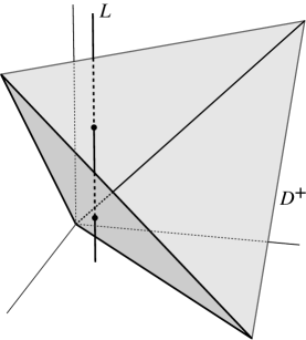
Figure 1. Model space transitions in sidelength space

Thus $L$ is the union of three closed segments, intersecting only at their two endpoints on $D^{+}$. We have just seen that the included angle function is decreasing on each segment, since the realizing triangles are in the same model space (by choice at the endpoints and by necessity elsewhere). Since the values at the endpoints are the same from left or right, the included angle function is decreasing on all of $L$. Similarly, each shoulder angle function is increasing.

Suppose $K>0$. The vertices of a triangle in the quadric model space are also the vertices of a triangle in an ambient $2$-plane, whose sides are the chords of the original sides. The length of the chord is an increasing function of the original sidelength. Thus to derive the lemma for $K>0$ from (2.1) and (2.2), we must verify the following: If a triangle in a quadric model space varies with fixed sidelengths adjacent to one vertex, and $v_{1},\,v_{2}$ are the tangent vectors to the sides at that vertex, then $<v_{1},v_{2}>$ is an increasing function of $<A_{1},A_{2}>$ where the $A_{i}$ are the chordal vectors of the two sides. Indeed, all points of a distance circle of nonzero radius in the quadric model space lie at a fixed nonzero ambient distance from the tangent plane at the centerpoint. Thus $A_{i}$ is a linear combination of $v_{i}$ and a fixed normal vector $N$ to the tangent plane, where the coefficients depend only on the sidelength $\ell_{i}$. The desired correlation follows.

By switching the sign of the metric, we obtain the claim for $K<0$. ∎

Remark 2.3.

The Law of Cosines in a semi-Riemannian model space with $K=0$ is (2.1). If $K\neq 0$, the Law of Cosines for $\triangle pqr$ may be written in unified form as follows:

(2.3) $$\cos\sqrt{KE(\gamma_{pr})}=\cos\sqrt{KE(\gamma_{pq})} \cos\sqrt{KE(\gamma_{qr})}$$

$$-K\angle pqr\frac{\sin\sqrt{KE(\gamma_{pq})}}{\sqrt{KE(\gamma_{pq})}}\frac{\sin\sqrt{KE(\gamma_{qr})}}{\sqrt{KE(\gamma_{qr})}}.$$

Here we assume $\triangle pqr$ satisfies the size bounds for $K$. Then each sidelength is $<\pi/\sqrt{K}$ if $K>0$, and $>-\pi/\sqrt{-K}$ if $K<0$. Part 1 of Lemma 2.2 can be derived from (2.3) as follows. Fix $E(\gamma_{pq})$ and $E(\gamma_{qr})$, and observe that $\cos\sqrt{Kc}$ is decreasing in $c$ if $K>0$, regardless of the sign of $c$ and even as $c$ passes through $0$, and increasing in $c$ if $K<0$. The size bounds imply that the factors $\frac{\sin\sqrt{Ka}}{\sqrt{Ka}}$ become either $\frac{\sin\sqrt{Ka}}{\sqrt{Ka}}$ for $\sqrt{Ka}\in[0,\pi)$, or $\frac{\sinh\sqrt{|Ka|}}{\sqrt{|Ka|}}$, depending on the signs of $K$ and $a$, and hence are nonnegative.

Now we are ready to prove a semi-Riemannian version of Alexandrov’s Straightening Lemma, according to which a triangle inherits comparison properties from two smaller triangles that subdivide it. It turns out that the comparisons we need are on nonnormalized shoulder angles. Moreover, the original and “subdividing” triangles may lie in varying model spaces, so that geometrically we have come a long way from the original interpretation in terms of hinged rods.

Since geodesics are parametrized by $[0,1]$, a point $m$ on a directed side of a triangle inherits an affine parameter $\lambda_{m}\in[0,1]$.

Lemma 2.4 (Straightening Lemma for Shoulder Angles).

Suppose $\triangle\widetilde{p}\widetilde{q}\widetilde{r}$ is a triangle satisfying size bounds for $K$ in a model space of curvature $K$. Let $\widetilde{m}$ be a point on side $\widetilde{p}\,\widetilde{r}$, and set $\lambda=\lambda_{\widetilde{m}}$. Let $\triangle q_{1}p_{1}m_{1}$ and $\triangle q_{2}m_{2}r_{2}$ be triangles in respective model spaces of curvature $K$, where $|q_{1}m_{1}|=|q_{2}m_{2}|=|\widetilde{q}\widetilde{m}|$, $|q_{1}p_{1}|=|\widetilde{q}\,\widetilde{p}|$, $|q_{2}r_{2}|=|\widetilde{q}\,\widetilde{r}|$, $|p_{1}m_{1}|=|\widetilde{p}\widetilde{m}|$, and $|m_{2}r_{2}|=|\widetilde{m}\widetilde{r}|$. Assume $|q_{i}m_{i}|<\pi/\sqrt{K}$ if $K>0$, and $|q_{i}m_{i}|>-\pi/\sqrt{-K}$ if $K<0$. If

$$(1-\lambda)\,\angle p_{1}m_{1}q_{1}+\lambda\,\angle r_{2}m_{2}q_{2}\geq 0,$$

then

$$\angle\widetilde{q}\,\widetilde{p}\widetilde{m}\geq\angle q_{1}p_{1}m_{1}\;\textit{ and }\;\angle\widetilde{q}\,\widetilde{r}\widetilde{m}\geq\angle q_{2}r_{2}m_{2}.$$

The same statement holds with all inequalities reversed.

Proof.

By the definition of nonnormalized angles, $(1-\lambda)\,\angle\widetilde{q}\widetilde{m}\widetilde{p}+\lambda\,\angle\widetilde{r}\widetilde{m}\widetilde{p}=0$. Therefore, by hypothesis, either $\angle q_{1}m_{1}p_{1}\geq\angle\widetilde{q}\widetilde{m}\widetilde{p}$ or $\angle r_{2}m_{2}p_{2}\geq\angle\widetilde{q}\widetilde{m}\widetilde{p}$. By Lemma 2.2.2, the inequality $|p_{i}m_{i}|\geq|\widetilde{p}\widetilde{m}|$ holds for either $i=1$ or $i=2$, and hence for both. But then by Lemma 2.2.1, the claim follows. ∎

3. Modified distance functions on model spaces

In this section we give a unified proof that in the model spaces of curvature $K$, the restrictions to geodesics $\gamma$ of the modified distance functions $h_{K,q}$ defined by (1.6) satisfy the differential equation

(3.1) $$(h_{K,q}\circ\gamma)^{\prime\prime}+K\langle\gamma^{\prime},\gamma^{\prime}\rangle h_{K,q}\circ\gamma=\langle\gamma^{\prime},\gamma^{\prime}\rangle.$$

We begin by constructing the $K$-affine functions on the model spaces. For intrinsic metric spaces the notion of a $K$-affine function was considered in [AB1] and their structural implications were pursued in [AB2]. For semi-Riemannian manifolds the definition should be formulated to account for the causal character of geodesics, as follows.

Definition 3.1.

A $K$-affine function on a semi-Riemannian manifold is a real-valued function $f$ such that for every geodesic $\gamma$ the restriction satisfies

(3.2) $$(f\circ\gamma)^{\prime\prime}+K\langle\gamma^{\prime},\gamma^{\prime}\rangle f=0.$$

We say $f$ is $K$-concave if “$\leq 0$” holds in (3.2), and $K$-convex if “$\geq 0$” holds.

(Elsewhere we have called the latter classes $\mathcal{F}(K)$-concave/convex.)

As in the Riemannian case, the $n$-dimensional model spaces of curvature $K$ carry an $n+1$-dimensional vector space of $K$-affine functions, namely, the space of restrictions of linear functionals in the ambient semi-Euclidean space of a quadric surface model.

Specifically, let $\mathbf{R}^{n+1}_{k}$ be the semi-Euclidean space of index $k$. For $K\neq 0$, set $Q_{K}=\{p\in\mathbf{R}^{n+1}_{k}:\langle p,p\rangle=\frac{1}{K}\}$, with the induced semi-Riemannian metric, so that $Q_{K}$ is an $n$-dimensional space of constant curvature $K$. (The $2$-dimensional model spaces $M_{K}$ are the universal covers of such quadric surfaces.) For $q\in Q_{K}$, let $\ell_{K,q}:Q_{K}\to\mathbf{R}$ be the restriction to $Q_{K}$ of the linear functional on $\mathbf{R}^{n+1}_{k}$ dual to the element $q$, namely, $\ell_{K,q}(p)=\langle q,p\rangle$. Define $E_{q}$ on $Q_{K}$ by (1.5).

Proposition 3.2.

For $K\neq 0$, the function $\ell_{K,q}$ on $Q_{K}$ is $K$-affine. For any $p$ that is joined to $q$ by a geodesic in $Q_{K}$,

$$\ell_{K,q}(p)=\frac{1}{K}\cos\sqrt{KE_{q}(p)},$$

where the argument of cosine may be imaginary.

Proof.

We use the customary identification of elements of $\mathbf{R}^{n+1}_{k}$ with tangent vectors to $\mathbf{R}^{n+1}_{k}$and $Q_{K}$. Then the gradient of the linear functional $\langle q,\cdot\rangle$ on $\mathbf{R}^{n+1}_{k}$ is $q$, viewed as a parallel vector field. For $p\in Q_{K}$, projection $\pi_{p}:T_{p}\mathbf{R}^{n+1}_{k}\to T_{p}Q_{K}$ is given by $\pi_{p}(v)=v-K\langle v,p\rangle p$. In particular, $\pi_{p}p=0$. It is easily checked that $\operatorname{grad}_{p}\ell_{K,q}=\pi_{p}q$.

The connection $\nabla$ of $Q_{K}$ is related to the connection $D$ of $\mathbf{R}^{n+1}_{k}$ by projection, that is, $\nabla_{v}X=\pi_{p}D_{v}X$ for $v\in T_{p}Q_{K}$. Writing $p=\gamma(t)$, $v=\gamma^{\prime}(t)$ for a geodesic $\gamma$ of $Q_{K}$, then

$$(\ell_{K,q}\circ\gamma)^{\prime\prime}(t)=\langle\nabla_{v}\operatorname{grad}\ell_{K,q},v\rangle =\langle\pi_{p}D_{v}\pi_{p}q,v\rangle$$

$$=\langle\pi_{p}D_{v}(q-K\langle q,p\rangle p),v\rangle$$

$$=\langle\pi_{p}(0-K\langle q,v\rangle p-K\langle q,p\rangle\nabla_{v}p),v\rangle$$

(3.3) $$=-K\langle v,v\rangle\ell_{K,q}(\gamma(t)).$$

Thus $\ell_{K,q}$ is $K$-affine.

Since $q$ is orthogonal to the tangent plane $T_{q}Q_{K}$, the derivatives of $\ell_{K,q}$ at $q$ are all $0$. Along a geodesic $\gamma$ in $Q_{K}$ that starts at $q$, the initial conditions for $\ell_{K,q}\circ\gamma$ are $\ell_{K,q}(q)=1/K$, $(\ell_{K,q}\circ\gamma)^{\prime}(v)=0$, so the formula for $\ell_{K,q}\circ\gamma(t)$ is $\cos(\sqrt{K\langle v,v\rangle}\,t)/K$. ∎

For the case $K=0$ we consider the quadric surface model to be a hyperplane not through the origin, so that the affine functions on it are trivially the restrictions of linear functionals.

On a model space $Q_{K}$ of curvature $K\neq 0$, the modified distance function $h_{K,q}$ defined by (1.6) may be written on its domain as

(3.4) $$h_{K,q}=-\ell_{K,q}+1/K,$$

and satisfies the same differential equation along geodesics as $\ell_{K,q}$ except for an additional constant term, that is, $h_{K,q}$ satisfies (3.1). It is trivial to check that this equation holds when $K=0$ and $h_{K,q}=E_{q}/2$.

4. Ricatti comparisons for modified shape operators

In a given semi-Riemannian manifold $M$, set $h=h_{K,q}$ (as in (1.6)) for some fixed choice of $K$ and $q$. Define the modified shape operator $S=S_{K,q}$, on the region where $h$ is smooth, to be the self-adjoint operator associated with the Hessian of $h$, namely,

(4.1) $$Sv=\nabla_{v}\operatorname{grad}h.$$

The form of $h$ was chosen so that in a model space $Q_{K}$, $S$ is always a scalar multiple of the identity. Indeed, at any point in $Q_{K}$,

(4.2) $$S=\begin{cases}I,\quad&\text{if \,}K=0,\\ K\ell_{K,q}\cdot I,\quad&\text{if \,}K\neq 0,\end{cases}$$

where the latter equality is by Proposition 3.2 and (3.3).

Below, our Riccati equation (4.3) along radial geodesics $\sigma$ from $q$ differs from the standard one in [AH] and [Kr], being adjusted to facilitate the proof of Theorem 1.1. Thus it applies even if $\sigma$ is null; it concerns an operator $S$ that is defined on the whole tangent space; when $\sigma$ is nonnull, the restriction of $S$ to the normal space of $\sigma$ does not agree with the second fundamental form of the equidistant hypersurface but rather with a rescaling of it; and we do not differentiate with respect to an affine parameter along $\sigma$, but rather use the integral curve parameter of $\operatorname{grad}h$.

The gradient vector field $G=\operatorname{grad}h$ is tangent to the radial geodesics from $q$. Note that $G$ is nonzero along null geodesics radiating from $q$ even though $h$ vanishes along such geodesics. Specifically, $G$ may be expressed in terms of $\operatorname{grad}E_{q}$ on a normal coordinate neighborhood via (1.6). Here $\operatorname{grad}E_{q}=2P$, where $P$ is the image under $d\exp_{q}$ of the position vector field $v\mapsto v_{v}$ on $T_{q}M$ (see [O’N, p. 128]). If $K=0$, then $G=P$, and an affine parameter $t$ on a radial geodesic from $q$ is given in terms of the integral curve parameter $u$ of $G$ by $t=ae^{u}$ with $u=-\infty$ at $0$. If $K\neq 0$, then $G=(\sin\sqrt{KE_{q}}/\sqrt{KE_{q}})P$, so $G$ agrees with $P$ up to higher order terms, and the dominant term at $q$ in the integral curve expression is an exponential.

Let $R_{G}$ be the self-adjoint Ricci operator, $R_{G}v=R(G,v)G$. We are going to establish comparisons on modified shape operators, governed by comparisons on Ricci operators. Since we are interested in comparisons along two given geodesics, each radiating from a given basepoint, the effect of restricting to normal coordinate neighborhoods in the following proposition is merely to rule out conjugate points along both geodesics.

Proposition 4.1.

In a semi-Riemannian manifold $M$, on a normal coordinate neighborhood of $q$, the modified shape operator $S$ satisfies the first-order PDE

(4.3) $$\nabla_{G}S+S^{2}-(1-Kh)S+R_{G}+Kdh\otimes G=0.$$

Before verifying Proposition 4.1, we shift to the general setting of systems of ordinary differential equations in order to summarize all we need about Jacobi and Riccati equations.

Lemma 4.2.

For self-adjoint linear maps $R(t)$ on a semi-Euclidean space, suppose $F(t)$ satisfies

(4.4) $$F^{\prime\prime}(t)+R(t)F(t)=0$$

for $t\in[0,b]$, where $F(0)=0$,  $F^{\prime}(0)$ is invertible, and $F(t)$ is invertible for all $t\in(0,b]$. For a given function $g:[0,b]\to\mathbf{R}$ with $g(0)=0$,  $g^{\prime}(0)=1$, and $g>0$ on $(0,b]$, define $S$ by

(4.5) $$g(t)F^{\prime}(t)=S(t)F(t)\text{ for }t\in(0,b],$$

and

(4.6) $$S(0)=I.$$

Then $S$ is self-adjoint, smooth on $[0,b]$, and satisfies

(4.7) $$gS^{\prime}+S^{2}-g^{\prime}S+g^{2}R=0.$$

Proof.

Self-adjointness of $S$ follows from (4.4) and self-adjointness of $R$ (see [AH, p. 839]). By (4.5) and (4.4), on $(0,b]$ we have

$$S^{\prime}F+g^{-1}S^{2}F =S^{\prime}F+SF^{\prime}=g^{\prime}F^{\prime}+gF^{\prime\prime}$$

$$=g^{\prime}F^{\prime}-gRF=g^{\prime}g^{-1}SF-gRF.$$

Multiplying the first and last expressions by $gF^{-1}$ on the right yields (4.7).

On $[0,b]$ we have $g=t\overline{g}$ where $\overline{g}(0)=g^{\prime}(0)=1$, and $F=t\overline{F}$ where $\overline{F}(0)=F^{\prime}(0)$ is invertible. Then (4.5) gives $t\overline{g}F^{\prime}=St\overline{F}$ on $(0,b]$. By (4.6), $S=\overline{g}F^{\prime}\overline{F}^{-1}$ on $[0,b]$, so $S$ is smooth there. ∎

Comparisons of solutions of (4.7) will be in terms of the notion of positive definite and positive semi-definite self-adjoint operators [AH, p. 838]. A linear operator $A$ on a semi-Euclidean space is positive definite if $\langle Av,v\rangle>0$ for every $v\neq 0$, positive semi-definite if $\langle Av,v\rangle\geq 0$. We then write $A<B$ if $B-A$ is positive definite, and similarly for $A\leq B$. Note that the identity map $I$ is not positive definite if the index is positive; however, the eigenvalues of a positive definite operator $A$ are real. If $A\geq 0$ and $\langle Av,v\rangle=0$, then $Av=0$.

In [AH, p. 846-847], a comparison theorem for the shape operators of tubes in semi-Riemannian manifolds is stated without proof. For the proof of Theorem 1.1 we require a stronger version of the special case in which the central submanifolds are just points, so the shape operators of distance-spheres are compared; the strengthening comes from the extension to modified shape operators. Since it is a key result for us, we now show how this version can be derived from a modification of the comparison theorem proved in [AH, p. 838-841], together with a Taylor series argument to cover the behavior at the base-point singularity.

Theorem 4.3.

Let $g$ and $R_{i},\,F_{i},\,S_{i}$ ($i=1,2$) be as in Lemma 4.2, and assume $g^{\prime\prime}(0)=0$. If $R_{1}(t)\leq R_{2}(t)$ for all $t\in[0,b]$, then $S_{1}(t)\geq S_{2}(t)$ on $[0,b]$. If $S_{1}(b)=S_{2}(b)$, then $R_{1}(t)=R_{2}(t)$ on $[0,b]$.

Proof.

First we show that (4.7) and the initial data for $g$ imply

(4.8) $$S^{\prime}(0)=0$$

and

(4.9) $$S^{\prime\prime}(0)=\frac{1}{3}(g^{\prime\prime\prime}(0)I-2R(0)).$$

To see this, differentiate (4.7), obtaining

$$g^{\prime}S^{\prime}+gS^{\prime\prime}+S^{\prime}S+SS^{\prime}-g^{\prime\prime}S-g^{\prime}S^{\prime}+(g^{2}R)^{\prime}=0.$$

Applying the initial data for $g$ and $S(0)=I$ gives (4.8). Now cancel the $\pm g^{\prime}S^{\prime}$ terms and differentiate again:

$$g^{\prime}S^{\prime\prime}+gS^{\prime\prime\prime}+2{S^{\prime}}^{2}+SS^{\prime\prime}+S^{\prime\prime}S-g^{\prime\prime\prime}S-g^{\prime\prime}S^{\prime}+(g^{2}R)^{\prime\prime}=0.$$

Setting $t=0$ gives (4.9).

Now for $\delta>0$, let $R_{\delta}=R_{2}+\delta B$, where $B$ is a positive definite self-adjoint operator, constant as a function of $t$. The solutions $F_{\delta}$ of $F^{\prime\prime}+R_{\delta}F=0$ with $F_{\delta}(0)=0$ and $F_{\delta}^{\prime}(0)=F_{2}^{\prime}(0)=\overline{F_{2}}(0)$ depend continuously on the parameter $\delta$, approaching the solution $F_{2}$ of $F^{\prime\prime}(t)+R_{2}F=0$. In particular, $F_{\delta}(t)$ is invertible for all $t\in[0,b]$ if $\delta$ is sufficiently small. Define $S_{\delta}(t)$ as in (4.4),  (4.5) with $R=R_{\delta}$.

Since $R_{\delta}(0)>R_{2}(0)\geq R_{1}(0)$, setting $S=S_{\delta}$ and $S=S_{1}$ in (4.9) implies $S_{1}^{\prime\prime}(0)>S_{\delta}^{\prime\prime}(0)$. Since $S_{1}(0)=I=S_{\delta}(0)$, and $S_{1}^{\prime}(0)=0=S_{\delta}^{\prime}(0)$ by (4.8), then $S_{1}(t)>S_{\delta}(t)$ for all $t\in(0,a)$, where $a>0$ depends on $\delta$.

But then $S_{1}(t)>S_{\delta}(t)$ for $t\in(0,b]$. Our argument for this follows [AH, p. 839], except for showing that the additional linear term in (4.7) is harmless. Namely, assume the statement is false. Then there exists $t_{0}\in(a,b]$ for which $S_{1}(t_{0})\geq S_{\delta}(t_{0})$, $S_{1}(t_{0})-S_{\delta}(t_{0})$ is not positive definite, and $S_{1}(t)>S_{\delta}(t)$ for $t<t_{0}$. Hence there is a nonzero vector $x_{0}$ such that $\langle(S_{1}(t_{0})-S_{\delta}(t_{0}))x_{0},x_{0}\rangle=0$, and so $S_{1}(t_{0})x_{0}=S_{\delta}(t_{0})x_{0}$. For $f(t)=\langle(S_{1}(t)-S_{\delta}(t))x_{0},x_{0}\rangle$, then by (4.7),

$$g(t_{0})f^{\prime}(t_{0}) =\langle(g(t_{0})S_{1}^{\prime}(t_{0})-g(t_{0})S_{\delta}^{\prime}(t_{0}))x_{0},x_{0}\rangle$$

$$=\langle S_{\delta}(t_{0})x_{0},S_{\delta}(t_{0})x_{0}\rangle-\langle S_{1}(t_{0})x_{0},S_{1}(t_{0})x_{0}\rangle$$

$$+\langle g^{\prime}(t_{0})(S_{1}(t_{0})-S_{\delta}(t_{0}))x_{0},x_{0}\rangle+g(t_{0})^{2}\langle(R_{\delta}(t_{0})-R_{1}(t_{0}))x_{0},x_{0}\rangle$$

$$=g(t_{0})^{2}\langle(R_{\delta}(t_{0})-R_{1}(t_{0}))x_{0},x_{0}\rangle>0.$$

This contradicts $g(t_{0})f^{\prime}(t_{0})\leq 0$, which is true because $f(t)>0$ on $(a,t_{0})$ and $f(t_{0})=0$.

Since $S_{1}(t)>S_{\delta}(t)$ for all $t\in(0,b]$, and $S_{\delta}(t)\to S_{2}(t)$ for all $t\in[0,b]$, we have $S_{1}(t)\geq S_{2}(t),\,t\in[0,b]$. ∎

Returning to the geometric setting, let us verify Proposition 4.1.

Proof of Proposition 4.1. Let $N$ be the unit radial vector field tangent to nonnull geodesics from $q$. By continuity, it suffices to verify (4.3) at every point that is joined to $q$ by a nonnull geodesic $\sigma$.

First we check that (4.3) holds when applied to $\sigma^{\prime}=N$. Note that the modified shape operator $S$ satisfies

(4.10) $$SN=\nabla_{N}G=(1-Kh)N.$$

Indeed, the form of $\nabla_{N}G$ along a unitspeed radial geodesic from the basepoint is the same in all manifolds, hence the same in $M$ as in a model space. But in a model space, (4.2) and (3.4) imply $\nabla_{N}G=SN=K\ell_{K,q}N=(1-Kh)N$. Therefore

$$(\nabla_{G}S+ S^{2}-(1-Kh)S+R_{G}+Kdh\otimes G)N$$

$$=-K(Gh)N+(1-Kh)^{2}N-(1-Kh)^{2}N+0+K(Nh)G$$

$$=-Kg(Nh)N+K(Nh)gN=0,$$

as required.

Now we verify that (4.3) holds on $V=V_{\sigma(t)}=\sigma^{\prime}(t)^{\perp}$. If $M$ has dimension $n$ and index $k$, consider an isometry $\varphi:T_{q}M\to\mathbf{R}_{k}^{n}$. For a nonnull, unitspeed geodesic $\sigma$ in $M$ radiating from $q$, identify $T_{\sigma(t)}M$ with $\mathbf{R}_{k}^{n}$ by parallel translation to the base point composed with $\varphi$. Thus we identify linear operators on $T_{\sigma(t)}M$ and $\mathbf{R}_{k}^{n}$, and likewise on $V_{\sigma(t)}$ and the corresponding $(n-1)$-dimensional subspace of $\mathbf{R}_{k}^{n}$. If we restrict to $V=V_{\sigma(t)}$, and set $R=R_{\sigma^{\prime}}$ and $g=1$, then (4.4) becomes the Jacobi equation for normal Jacobi fields, and the operator defined by (4.5) is $S(t)=W(t)$, the Weingarten operator, for $t>0$:

$$Wv=\nabla_{v}N,\,v\in V.$$

(See [AH], which uses the opposite sign convention for $W$.) If instead we set $R=R_{\sigma^{\prime}}$ as before but $g=|<G,G>|^{\frac{1}{2}}$ where $G=\operatorname{grad}h$, so that $G=gN$ and $vg=0$ for $v\in V$, then the operator $S(t)$ defined by (4.5) and (4.6) is the restriction to $V$ of the modified shape operator, for $t\geq 0$. Indeed, (4.5) implies $S(t)=g(t)W(t)$ for $t>0$, hence

$$Sv=g\nabla_{v}N=\nabla_{v}(gN)=\nabla_{v}G,$$

which agrees with the definition (4.1) of the modified shape operator. And the modified shape operator is the identity at $q$ by (4.10), since $N$ can be chosen to be any unit vector at $q$. Then it is straightforward from (4.7) that the restriction to $V$ of the modified shape operator satisfies (4.3).

The proof of the rigidity statement proceeds just as in [AH, p. 840]. ∎

Remark 4.4.

To summarize, [AH, Theorem 3.2] applies to the Weingarten operator of the equidistant hypersurfaces from a hypersurface. In that case, both $R$ and $W(0)$ are perturbed in order to obtain a strict inequality on operators; if instead we considered the modified Weingarten operator $S=gW$, so $S(0)=0$, we would perturb $R$ and $S^{\prime}(0)$. On the other hand, Theorem 4.3 above applies to $gW$, where $W$ is the Weingarten operator of the equidistant hypersurfaces from a point. Here we had $S(0)=I$ and $S^{\prime}(0)=0$, and showed that merely perturbing $R$ implied a desired perturbation of $S^{\prime\prime}(0)$ and hence of $S(a)$ for small $a$. The theorem stated without proof in [AH, p.846-847] applies to the intermediate case of equidistant hypersurfaces from any submanifold $L$. Except for changes in details, our proof above works for that case as well.

Now let us compare modified shape operators via Theorem 4.3. We say two geodesic segments $\sigma$ and $\widetilde{\sigma}$ in semi-Riemannian manifolds $M$ and $\widetilde{M}$ correspond if they are defined on the same affine parameter interval and satisfy $\langle\sigma^{\prime},\sigma^{\prime}\rangle=\langle\widetilde{\sigma}^{\prime},\widetilde{\sigma}^{\prime}\rangle$.

Corollary 4.5.

For semi-Riemannian manifolds $M$ and $\widetilde{M}$ of the same dimension and index, suppose $\sigma$ and $\widetilde{\sigma}$ are corresponding nonnull geodesic segments radiating from the basepoints $q\in M$ and $\widetilde{q}\in\widetilde{M}$ and having no conjugate points. Identify linear operators on $T_{\sigma(t)}M$ with those on $T_{\widetilde{\sigma}(t)}\widetilde{M}$ by parallel translation to the basepoints, together with an isometry of $T_{q}M$ and $T_{\widetilde{q}}\widetilde{M}$ that identifies $\sigma^{\prime}(0)$ and $\widetilde{\sigma}^{\prime}(0)$. If $R_{\sigma^{\prime}}\geq\widetilde{R}_{\widetilde{\sigma}^{\prime}}$ at corresponding points of $\sigma$ and $\widetilde{\sigma}$, then the modified shape operators satisfy $S\leq\widetilde{S}$ at corresponding points of $\sigma$ and $\widetilde{\sigma}$.

Proof.

The modified shape operators split into direct summands, corresponding to their action on the one-dimensional spaces tangent to the radial geodesics and on the orthogonal complements $V$. The first summand is the same for both $M$ and $\widetilde{M}$. The second summand is as described in Lemma 4.2 with $R=R_{\sigma^{\prime}}$ and $g=|<G,G>|^{\frac{1}{2}}$. (Since our identification of $T_{\sigma(t)}M$ and $T_{\widetilde{\sigma}(t)}\widetilde{M}$ identifies $G$ and $\widetilde{G}$, we denote both of these by $G$.) Furthermore, $g^{\prime}=1-Kh$ by (4.10), so $g^{\prime\prime}(0)=0$ by (1.6). Therefore the corollary follows from Theorem 4.3. ∎

Corollary 4.6.

Suppose $M$ is a semi-Riemannian manifold satisfying $R\geq K$, and $\widetilde{M}=Q_{K}$ has the same dimension and index as $M$ and constant curvature $K$. Then for any $p\in M$ that is joined to $q$ by a geodesic that has no conjugate points and such that a corresponding geodesic segment in $\widetilde{M}$ has no conjugate points, the modified shape operator $S=S_{K,q}$ satisfies

(4.11) $$S(p)\leq(1-Kh_{K,q}(p))\cdot I.$$

The same statement holds with inequalities reversed.

Proof.

Let $\sigma$ be the given geodesic from $q$ to $p=\sigma(t)$, and $\widetilde{\sigma}$ be a corresponding geodesic from $\widetilde{q}\in\widetilde{M}$ to $\widetilde{p}=\widetilde{\sigma}(t)$. If $\sigma$ is nonnull, then by Corollary 4.5, (4.2) and (3.4), we have

$$S(p)\leq\widetilde{S}(\widetilde{p}) =K\ell_{K,\widetilde{q}}(\widetilde{p})\cdot\widetilde{I}$$

$$=(1-K\widetilde{h}_{K,\widetilde{q}}(\widetilde{p}))\cdot\widetilde{I},$$

where $\widetilde{I}$ denotes the identity operator on $T_{\widetilde{p}}\widetilde{M}$, and $T_{p}M,\,T_{\widetilde{p}}\widetilde{M}$ are identified by parallel translation to $q,\,\widetilde{q}$ followed by an isometry identifying $\sigma^{\prime}(0),\,\widetilde{\sigma}^{\prime}(0)$. Corollary 4.5 applies here because the righthand side of (1.1) is $\widetilde{R}(v,w,v,w)$, and so $R_{\sigma^{\prime}}\leq\widetilde{R}_{\widetilde{\sigma}^{\prime}}$ at corresponding points of $\sigma$ and $\widetilde{\sigma}$. Since $\widetilde{h}_{K,\widetilde{q}}(\widetilde{p})=h_{K,q}(p)$, then (4.11) holds at $p$. Therefore (4.11) holds everywhere by continuity. ∎

5. Proof of Theorem 1.1

Now we are ready to prove that in a semi-Riemannian manifold $M$, triangle comparisons hold in any normal neighborhood $U$ in which there is a curvature bound $K$ and triangles satisfy size bounds for $K$. By the Realizability Lemma, such a $\triangle pqr$ has a model triangle $\triangle\widetilde{p}\,\widetilde{q}\,\widetilde{r}$, which in this section we embed in $Q_{K}$, where $Q_{K}$ is taken of the same dimension and index as $U$.

There are several equivalent formulations of the triangle comparisons we seek:

Proposition 5.1.

The following conditions on all triangles in $U$ are equivalent:

• The signed distance between any two points is $\geq$ ($\leq$) the signed distance between the corresponding points in the model triangle.

• The signed distance from any vertex to any point on the opposite side is $\geq$ ($\leq$) the signed distance between the corresponding points in the model triangle.

• The nonnormalized angles are $\leq$ ($\geq$) the corresponding nonnormalized angles of the model triangle.

Proof.

$1$ obviously implies $2$. Conversely, for $\triangle pqr$ in $U$, suppose $m$ is on side $\gamma_{pr}$ and $n$ is on side $\gamma_{pq}$, and $\lambda_{m}$ and $\lambda_{n}$ are the corresponding affine parameters. Let $\triangle\widetilde{p}\,\widetilde{q}\widetilde{r}$ be the model triangle for $\triangle pqr$, $\triangle\widetilde{p}^{\prime}\,\widetilde{m}^{\prime}\widetilde{q}^{\prime}$ be the model triangle for $\triangle pmq$, and $\triangle\overline{p}\,\overline{m}\,\overline{n}$ be the model triangle for $\triangle pmn$. Let $\widetilde{m}$ on $\gamma_{\widetilde{p}\,\widetilde{r}}$ and $\widetilde{n}$ on $\gamma_{\widetilde{p}\,\widetilde{q}}$ have affine parameters $\lambda_{m}$ and $\lambda_{n}$, and similarly for $\widetilde{n}^{\prime}$ on $\gamma_{\widetilde{p}^{\prime}\,\widetilde{q}^{\prime}}$. By 2, $|\overline{m}\,\overline{n}|=|mn|\geq|\widetilde{m}^{\prime}\widetilde{n}^{\prime}|$. Therefore by Lemma 2.2.1 (Hinge),

(5.1) $$\angle\overline{m}\,\overline{p}\,\overline{n}\leq\angle\widetilde{m}^{\prime}\,\widetilde{p}^{\prime}\,\widetilde{n}^{\prime}.$$

Again by 2, $|\widetilde{m}^{\prime}\,\widetilde{q}^{\prime}|=|mq|\geq|\widetilde{m}\,\widetilde{q}|$. By Hinge applied to $\triangle pmq$, together with (5.1), we have

(5.2) $$\angle\overline{m}\,\overline{p}\,\overline{n}\leq\angle\widetilde{m}^{\prime}\,\widetilde{p}^{\prime}\,\widetilde{n}^{\prime}\leq\angle\widetilde{m}\,\widetilde{p}\,\widetilde{n}.$$

Again by Hinge, $|mn|=|\overline{m}\,\overline{n}|\geq|\widetilde{m}\,\widetilde{n}|$, and so 2 implies 1.

The implication $2\Rightarrow 3$ is a direct consequence of the first variation formula (see [O’N, p. 289]):

(5.3) $$(E_{q}\circ\gamma_{pr})^{\prime}(0)=2\angle qpr.$$

(Note that our definition of $E$ and O’Neill’s differ by a factor of $2$.)

Conversely, using the same triangle notation as above, 3 gives $\angle pmq\leq\angle\widetilde{p}^{\prime}\,\widetilde{m}^{\prime}\,\widetilde{q}^{\prime}$, and similarly $\angle qmr\leq\angle\widetilde{q}^{\prime}\,\widetilde{m}^{\prime}\,\widetilde{r}^{\prime}$. Since $(1-\lambda_{m})\,\angle pmq+\lambda\,\angle qmr=0$, we have $(1-\lambda_{m})\angle\widetilde{p}^{\prime}\,\widetilde{m}^{\prime}\,\widetilde{q}^{\prime}+\lambda_{m}\angle\widetilde{q}^{\prime}\,\widetilde{m}^{\prime}\,\widetilde{r}^{\prime}\geq 0$. By Lemma 2.4 (Straightening), $\angle\widetilde{q}^{\prime}\,\widetilde{p}^{\prime}\widetilde{m}^{\prime}\leq\angle\widetilde{q}\,\widetilde{p}\widetilde{m}$. Therefore by Hinge, $|qm|=|\widetilde{q}^{\prime}\,\widetilde{m}^{\prime}|\geq|\widetilde{q}\,\widetilde{m}|$, and so 3 implies 2. ∎

Turning to the proof of Theorem 1.1, consider $\triangle pqr$ in $U$, and its model triangle $\widetilde{p}\,\widetilde{q}\,\widetilde{r}$, which we regard as lying in $\widetilde{M}=Q_{K}$. Taking $q$ and $\widetilde{q}$ as base points gives modified distance functions $h_{K,q}$ and $\widetilde{h}_{K,\widetilde{q}}$. For any $m\in U$, the signed distance $|qm|$ is a monotone increasing function of $h_{q}(m)$, and distances from $\widetilde{q}$ in $Q_{K}$ have exactly the same relation with $\widetilde{h}_{K,\widetilde{q}}$. Thus the following proposition shows that curvature bounds imply triangle comparisons in the sense of Proposition 5.1.2, thereby proving the “only if” part of Theorem 1.1.

Proposition 5.2.

Set $h=h_{K,q}\circ\gamma_{pr}$ and $\widetilde{h}=\widetilde{h}_{K,\widetilde{q}}\circ\widetilde{\gamma}_{\widetilde{p}\widetilde{r}}$.

If $R\geq K$ in $U$, then $h\geq\widetilde{h}$.

If $R\leq K$ in $U$, then $h\leq\widetilde{h}$.

Proof.

Assume $R\geq K$. Aside from reversing inequalities the proof for $R\leq K$ is just the same.

Set $\gamma=\gamma_{pr}$ and $\widetilde{\gamma}=\widetilde{\gamma}_{\widetilde{p}\widetilde{r}}$. For $m=\gamma(s)$, by Corollary 4.6, the modified shape operator $S=S_{K,q}$ satisfies

$$S(m)\leq(1-Kh_{K,q}(m))\cdot I.$$

Since, by definition, $\langle Sv,v\rangle$ is the second derivative of $h_{K,q}$ along the geodesic with velocity $v$, then

$$(h_{K,q}\circ\gamma)^{\prime\prime}(s)\leq(1-Kh_{K,q}(m))\langle\gamma^{\prime}(s),\gamma^{\prime}(s)\rangle.$$

That is, along $\gamma$, $h_{K,q}$ satisfies the differential inequality

$$h^{\prime\prime}+KE(\gamma)h\leq E(\gamma).$$

On the other hand, the above inequalities become equations in $Q_{K}$, so

$$\widetilde{h}^{\prime\prime}+KE(\widetilde{\gamma})\widetilde{h}=E(\widetilde{\gamma}).$$

But $E(\widetilde{\gamma})=E(\gamma)$ since $\widetilde{\gamma}$ is a model segment for $\gamma$. Hence the difference $f=h-\widetilde{h}$ is $KE(\gamma)$-concave:

$$f^{\prime\prime}+KE(\gamma)f\leq 0.$$

Moreover, at $0$ and $1$ the values of $h$ and $\widetilde{h}$ are the same since $E_{q}(p)=E_{\widetilde{q}}(\widetilde{p})$ and $E_{q}(r)=E_{\widetilde{q}}(\widetilde{r})$, so the end values of $f$ are just $f(0)=f(1)=0$. By concavity $f$ is bounded below by the $KE(\gamma)$-affine function with those end values, which is just $0$. That is, $f\geq 0$, or $h\geq\widetilde{h}$. ∎

Next we verify the “if” part of Theorem 1.1:

Proposition 5.3.

If signed distances between pairs of points on any triangle in $U$ are at least (at most) those between the corresponding points of the comparison triangle, then $R\geq K$ ($R\leq K$).

Proof.

Let $\sigma$ be a nonnull geodesic segment in $U$, let $v\in T_{\sigma(0)}M$ be nonnull and perpendicular to $\sigma^{\prime}(0)$, and let $J$ be the Jacobi field along $\sigma$ such that $J(0)=0,J^{\prime}(0)=v$. In the $2$-dimensional model space $\widetilde{M}$ of curvature $K$ and of the same signature as the section spanned by $\sigma^{\prime}(0)$ and $v$, choose a geodesic $\widetilde{\sigma}$ and vector $\widetilde{v}$ at $\widetilde{\sigma}(0)$ perpendicular to $\sigma^{\prime}(0)$ such that $\langle\widetilde{\sigma}^{\prime}(0),\widetilde{\sigma}^{\prime}(0)\rangle=\langle\sigma^{\prime}(0),\sigma^{\prime}(0)\rangle$ and $\langle\widetilde{v},\widetilde{v}\rangle=\langle v,v\rangle$. Let $\widetilde{J}$ be the Jacobi field on $\widetilde{\sigma}$ such that $\widetilde{J}(0)=0,\widetilde{J}^{\prime}(0)=v$.

Write

$$\tau(t,s)=\sigma_{s}(t)=\exp_{\sigma(0)}t(\sigma^{\prime}(0)+sv),$$

and similarly for $\widetilde{\tau}$. Since $\frac{\partial\tau}{\partial t}(0,s)=\sigma^{\prime}(0)+sv$, then $\langle\frac{\partial\tau}{\partial t}(0,0),\frac{\partial\tau}{\partial t}(0,s)\rangle$ is equal to the corresponding expression in $\widetilde{M}$. But then our triangle comparison assumption, in the form given in Proposition 5.1.3, and Lemma 2.2.1 (Hinge) combine to give $|\sigma_{0}(t)\sigma_{s}(t)|\leq|\widetilde{\sigma}_{0}(t)\widetilde{\sigma}_{s}(t)|.$ Since

$$|J(t)|=\lim_{s\to 0}|\sigma_{0}(t)\sigma_{s}(t)|/s,$$

and similarly in $\widetilde{M}$, we conclude

$$\langle J(t),J(t)\rangle\leq\langle\widetilde{J}(t),\widetilde{J}(t)\rangle.$$

Now we calculate the third order Taylor expansion of $J$.

$$J^{\prime\prime}=-R_{\sigma^{\prime}J}\gamma^{\prime},\quad J^{\prime\prime}(0)=0,$$

$$J^{\prime\prime\prime}=-R^{\prime}_{\gamma^{\prime}J}\gamma^{\prime}-R_{\gamma^{\prime}J^{\prime}}\gamma^{\prime},\quad J^{\prime\prime\prime}(0)=-R_{\gamma^{\prime}(0)v}\gamma^{\prime}(0),$$

and hence

$$J(t)=\mathcal{P}_{t}(vt-\frac{1}{6}R_{\gamma^{\prime}(0)v}\gamma^{\prime}(0)t^{3}+O(t^{4})),$$

where $\mathcal{P}_{t}$ is parallel translation from $\gamma(0)$ to $\gamma(t)$ and the primes indicate $\nabla_{\gamma^{\prime}(t)}$. Then we get an expansion

$$\langle J(t),J(t)\rangle=\langle v,v\rangle t^{2}-\frac{1}{3}\langle R_{\gamma^{\prime}(0)v}\gamma^{\prime}(0),v\rangle t^{4}+O(t^{5}),$$

and a similar expansion for $\langle\widetilde{J}(t),\widetilde{J}(t)\rangle$. Since the $t^{2}$-terms are the same, we must have the inequality for the $t^{4}$-terms:

$$\langle R_{\gamma^{\prime}(0)v}\gamma^{\prime}(0),v\rangle\geq\langle\widetilde{R}_{\widetilde{\gamma}^{\prime}(0)\,\widetilde{v}}\widetilde{\gamma}^{\prime}(0),v\rangle=K\langle\gamma^{\prime}(0),\gamma^{\prime}(0)\rangle\langle v,v\rangle.$$

Since $\gamma^{\prime}(0)$ and $v$ span an arbitrary nonnull section, $R\geq K$ follows. ∎

6. Algebraic meaning of curvature bounds

Curvature bounds of the type studied in this paper are clarified by the analysis by Beem and Parker of the pointwise ranges of sectional curvature [BP], as we now explain. We go further, to relate our curvature bounds to the “null” curvature bounds considered by Uhlenbeck [U] and Harris [H1].

Since in a semi-Riemannian manifold with indefinite metric, a spacelike section always lies in a Lorentz or anti-Lorentz $3$-plane $V$, the range of sectional curvature may be studied by restricting to such $3$-planes $V$. On $V$, unless the curvature is constant, both the time-like and space-like sections have infinite intervals as their range, and either both are the entire real line or both are rays which overlap in at most a common end (see Theorem 6.1). Then as we vary $V$ in the tangent bundle, either the separation between the two rays can be lost or we can have numbers that separate all pairs of intervals, namely, a curvature bound in our sense.

In this section, $V$ always denotes a Lorentz or anti-Lorentz $3$-plane. Following [BP], consider a curvature tensor $R$ on $V$. Express $R$ as a homogeneous quadratic form $v\wedge w\mapsto\mathcal{Q}_{1}(v\wedge w)=R(v,w,v,w)$ on $\bigwedge^{2}V$. If $(e_{1},e_{2},e_{3})$ is a frame for which $e_{2}$ and $e_{3}$ have the same signature, then $(e_{1}\wedge e_{2},e_{1}\wedge e_{3},e_{2}\wedge e_{3})$ is a frame for $\bigwedge^{2}V$ with signature $(-,-,+)$ with respect to the natural extension of the inner product. Every nonzero element $x_{1}e_{1}\wedge e_{2}+x_{2}e_{1}\wedge e_{3}+x_{3}e_{2}\wedge e_{3}$ of $\bigwedge^{2}V$ is decomposable, and so represents a oriented section of $V$, so the projective plane $\mathbf{P}^{2}$ of all nonorientable sections of $V$ has homogeneous coordinates $x_{1},x_{2},x_{3}$. The inner product quadratic form on $\bigwedge^{2}V$ has the coordinate expression $\mathcal{Q}_{2}=\langle v,v\rangle=(x_{3})^{2}-(x_{1})^{2}-(x_{2})^{2}$, and the sectional curvature function is $\mathcal{K}=\mathcal{Q}_{1}/\mathcal{Q}_{2}$. We also identify $\mathcal{Q}_{1}$ and $\mathcal{Q}_{2}$ with the quadratic functions on $\mathbf{P}^{2}-\{\ell_{\infty}\}$ given in terms of the corresponding nonhomogeneous coordinates $x=x_{1}/x_{3},\quad y=x_{2}/x_{3}$ by $\mathcal{Q}_{1}/(x_{3})^{2}$ and $\mathcal{Q}_{2}/(x_{3})^{2}=1-x^{2}-y^{2}$. For various curvature tensors there is no restriction on $\mathcal{Q}_{1}$; that is, for a given point $p$ in any $n$-dimensional manifold $M$, and a given $3$-dimensional subspace $V$ of $T_{p}M$, a semi-Riemannian metric with indefinite restriction to $V$ can be specified in a neighborhood of $p$ in terms of normal coordinates so as to realize any curvature tensor on $V$.

The null conic $N$ is given by $\mathcal{Q}_{2}=0$, and represents those sections of $V$ on which the inner product is degenerate and $\mathcal{K}=\mathcal{Q}_{1}/\mathcal{Q}_{2}$ is undefined. The homaloidal (flat) conic $H$ is given by $\mathcal{Q}_{1}=0$. The inclusion $N\subset H$ is equivalent to $\mathcal{K}$ being constant on the sections of $V$, which is to say, $\mathcal{Q}_{1}$ being $\mathcal{Q}_{2}$ multiplied by that constant value (which may be $0$ so the inclusion could be proper). Otherwise, $H$ and $N$ intersect in at most $4$ points, counting multiplicities. The points of odd multiplicity are precisely the points where $H$ and $N$ cross.

Since the interior and exterior of $N$ are connected sets on which $\mathcal{K}$ is continuous, the ranges of $\mathcal{K}$ on time-like sections and space-like sections of $V$ are intervals, $I_{ti}$ and $I_{sp}$. The following theorem characterizes the possible ranges. It implies, in particular, that if on $V$ either timelike or spacelike curvatures are bounded, then both are, and there exists a curvature bound in our sense.

Theorem 6.1 ([BP]).

For a curvature tensor on a Lorentz or anti-Lorentz $3$-plane:

• $\mathcal{K}$ is constant if $N\subset H$.

• $I_{sp}=I_{ti}=\mathbf{R}$ if $H$ and $N$ cross.

• $I_{sp}$ and $I_{ti}$ are oppositely directed closed half-lines, separated by a nontrivial open interval of curvature bounds, if $H$ does not intersect $N$ (including the cases when $H$ is empty or a point not in $N$).

• $I_{sp}$ and $I_{ti}$ are oppositely directed half-lines with a common endpoint otherwise, namely, when $H$ and $N$ have a point of tangency but never cross. More specifically, $I_{sp}$ and $I_{ti}$ are both open, both closed, or complementary, according as $H$ and $N$ intersect in a single point of order $2$, two points of order $2$, or a single point of order $4$.

In a semi-Riemannian manifold with indefinite metric, $R\geq K$ holds if and only if the restriction of the curvature tensor to each Lorentz or anti-Lorentz $3$-plane $V$ satisfies $R\geq K$ (and similarly for $R\leq K$). Equivalently, on each $V$, either $\mathcal{K}$ is constantly $K$, or $I_{ti}$ is a semi-infinite interval in $(-\infty,K]$ and $I_{sp}$ is a semi-infinite interval in $[K,\infty)$. Theorem 6.1 leads us to consider a weaker condition, which we denote by $R_{V}\geq K(V)$, in which the interval betweeen $I_{ti}$ and $I_{sp}$ varies with the indefinite $3$-plane $V$, and there may be no $K$ common to all.

Write $R_{null}\geq 0$ if $R(v,x,v,x)\geq 0$ for any null vector $x$ and non-zero vector $v$ perpendicular to $x$. It is shown in [H1, Proposition 2.3] (or see [BEE, Proposition A.7]) that if $R_{null}>0\,(<0)$ at a point, then the range of timelike sectional curvatures at that point is unbounded below (above). The following proposition gives precise information.

Proposition 6.2.

A semi-Riemannian manifold with indefinite metric satisfies $R_{null}\geq 0$ if and only if $R_{V}\geq K(V)$, and similarly with signs reversed.

Proof.

In a given Lorentz or anti-Lorentz $3$-plane $V$, the condition $R_{null}\geq 0$ is equivalent to $\mathcal{Q}_{1}\geq 0$ on the null conic $N$. In turn this implies that $N$ and $H$ do not cross, and hence cases 1, 3 or 4 of Theorem 6.1 hold. In case 1, obviously there is a lower curvature bound. In cases 3 and 4, there are points of $N$ at which $\mathcal{Q}_{1}>0$. Approaching $N$ from the spacelike side gives $R\to\infty$, so $I_{sp}$ is unbounded above and again $V$ has a lower curvature bound.

Conversely, suppose there is a lower curvature bound for $V$, so case 2 is ruled out. In case 1, $\mathcal{Q}_{1}=0$ on $N$. In cases 3 or 4, since $I_{sp}$ is bounded below, there cannot be points of $N$ at which $\mathcal{Q}_{1}<0$. ∎

The condition $R_{null}\leq 0$ plus a “growth condition” was used in [U] to prove a Hadamard-Cartan theorem for Lorentz manifolds. It seems interesting to investigate the relation between $R\leq 0$ and these hypotheses; Uhlenbeck comments about the growth condition,“it is to be hoped that a similar condition that does not depend on coordinates can be found” [U, p. 75].

The condition $R_{null}>0$ (or $<0$) isolates case 3 of Theorem 6.1. Now let us show how a strengthening of this condition bounds below the length of the interval of curvature bounds in each Lorentz or anti-Lorentz $3$-plane $V$.

While sectional curvature is undefined for null sections, Harris has used a substitute, relative to a choice of null vector $x$. Namely, for a null section $\Pi$ containing $x$, define the null curvature of $\Pi$ with respect to $x$ by

(6.1) $$\mathcal{K}_{x}(\Pi)=R(w,x,w,x)/\langle w,w\rangle$$

for any non-null vector $w$ in $\Pi$ [H1]. While there is no a priori way to normalize the null vector $x$, it is still possible to strengthen Proposition 6.2. This is because, in the presence of an interval of curvature bounds larger than a single point, the algebra of the curvature operator $\mathcal{R}:\bigwedge^{2}V\to\bigwedge^{2}V$ selects a distinguished timelike unit vector $t$, or “observer”, and hence a distinguished circle of null vectors $x$.

In the following proposition, we suppose $V$ is Lorentz (that is, has signature $(+,+,-)$). There are obvious sign changes if $-V$ is Lorentz.

Proposition 6.3.

Suppose there is an interval $[K_{1},K_{2}]$ of curvature bounds below on the Lorentz $3$-plane $V$, where $K_{1}<K_{2}$. Then $\mathcal{R}$ is diagonalizable. Let $t$ be a unit timelike vector perpendicular to the spacelike eigenbivector of $\mathcal{R}$. Then

(6.2) $$K_{2}-K_{1}=\min_{v}K_{x}(\Pi),$$

where $v$ runs over unit vectors perpendicular to $t$, and $x$ and $\Pi$ are the null vector and null section $x=t+v$ and $\Pi=x^{\perp}$ respectively. For curvature bounds above, substitute

(6.3) $$K_{1}-K_{2}=\max_{v}K_{x}(\Pi)$$

for (6.2).

Proof.

We consider the case of curvature bounds below. First observe that, while self-adjoint linear operators in indefinite inner product spaces are not always diagonalizable, our hypotheses imply diagonalizability. Indeed, the unit eigenbivectors of $\mathcal{R}$, of which one is spacelike and two are timelike, are the critical points of the corresponding quadratic form on unit bivectors. The values of this quadratic form are sectional curvatures, up to sign. Therefore $K_{2}$, the minimum spacelike sectional curvature, and $K_{1}$, the maximum timelike sectional curvature, are eigenvalues, which are distinct by hypothesis. The corresponding eigenbivectors span a nondegenerate $2$-dimensional subspace of $\bigwedge^{2}V$; a bivector perpendicular to both is an eigenbivector by self-adjointness. Thus our eigenbivectors diagonalize $\mathcal{R}$. Let $t,v_{1},v_{2}$ be a frame of vectors perpendicular to the eigensections, so that $t\wedge v_{1}$ and $t\wedge v_{2}$ are the timelike eigenbivectors. Then the null vectors $x=t+v$ have the form $t+\cos\theta v_{1}+\sin\theta v_{2}$, and the null curvatures $\mathcal{K}_{x}(\Pi)$ have the form $K_{2}-K_{1}\cos^{2}\theta-K_{3}\sin^{2}\theta$ where $K_{3}\leq K_{1}$. Thus the minimum is $K_{2}-K_{1}$. ∎

7. Warped product examples

If $B$ and $F$ are Riemannian manifolds, $(-B)\times_{f}F$ will denote the product manifold with the warped product metric $\langle\,,\,\rangle=-ds^{2}_{B}+f^{2}ds^{2}_{F}$. The sectional curvature $\mathcal{K}$ of $(-B)\times_{f}F$, in terms of the sectional curvatures $\mathcal{K}_{B}$ and $\mathcal{K}_{F}$, may be calculated for a frame $x+v,y+w$, for $x,y\in T_{p}B$ and $v,w\in T_{\overline{p}}F$. Without loss of generality, suppose $\langle x,y\rangle=\langle v,w\rangle=0$. Let $G$ be the gradient of $f$. Then

$$\mathcal{K}((x+v) \wedge(y+w))=-\mathcal{K}_{B}(x\wedge y)<x,x><y,y>$$

$$-f^{-1}(p)\left[<w,w>\nabla^{2}f(x,x)+<v,v>\nabla^{2}f(y,y)\right]$$

$$+f^{-2}(p)\left[\mathcal{K}_{F}(v\wedge w)-<G(p),G(p)>\right]<v,v><w,w>.$$

Therefore:

Proposition 7.1.

Consider Riemannian manifolds $B$ and $F$, and a smooth function $f:B\to\mathbf{R}_{>0}$. Then $(-B)\times_{f}F$ is a semi-Riemannian manifold satisfying $R\geq K$ ($R\leq K$) if and only if the following three conditions hold:

• $f$ is $(-K)$-concave   ($(-K)$-convex).

• $\dim B=1$ or $B$ has sectional curvature $\leq-K$ ($\geq K$),

• $\dim F=1$, or for all points $(p,\overline{p})$ and $2$-planes $\Pi_{\overline{p}}$ tangent to $F$,

  $\mathcal{K}_{F}(\Pi_{\overline{p}})\geq$ ($\leq$) $Kf(p)^{2}+<G(p),G(p)>$.

Taking $B$ to be an interval $I$ in Proposition 7.1, we easily construct a rich class of Lorentz examples:

Corollary 7.2.

If $f:I\to\mathbf{R}$ is $(-K)$-concave and $F$ is a Riemannian manifold of sectional curvature $\geq C$, then $(-I)\times_{f}F$ satisfies $R\geq K$ for any $K$ in the interval

(7.1) $$\left[\sup\frac{f^{\prime\prime}}{f},\,\inf\frac{C+(f^{\prime})^{2}}{f^{2}}\right].$$

If $f:I\to\mathbf{R}$ is $(-K)$-convex and $F$ is a Riemannian manifold of sectional curvature $\leq C$, then $(-I)\times_{f}F$ satisfies $R\leq K$ for any $K$ in the interval

(7.2) $$\left[\sup\frac{C+(f^{\prime})^{2}}{f^{2}},\,\inf\frac{f^{\prime\prime}}{f}\right].$$

Example 7.3.

Following [HE], by a Robertson-Walker space we mean a warped product $M=(-I)\times_{f}F$ where $F$ is $3$-dimensional spherical, hyperbolic or Euclidean space, say with curvature $C$. Then the sectional curvatures of sections containing $\partial/\partial t$ are $K_{-}(t)=\frac{f^{\prime\prime}(t)}{f(t)}$, and those of sections $\Pi$ tangent to the fiber are $K_{+}(t)=\frac{C+f^{\prime}(t)^{2}}{f(t)^{2}}$. By Corollary 7.2, $M$ satisfies $R\geq K$ if and only if $\sup K_{-}\leq\inf K_{+}$.

It is easy to check that a Robertson-Walker space satisfies the strong energy condition, $\operatorname{Ric}(t,t)\geq 0$ for all timelike vectors $t$, if and only if the curvature restricted to each tangent $4$-plane has a nonpositive curvature bound below in our sense (see [O’N, Exercise 10, p. 362]).

By the Einstein equation, taking the cosmological constant $\Lambda=0$, the stress-energy tensor of any Robertson-Walker space has the form of a perfect fluid whose energy density $\rho$ and pressure $p$ are functions of $t$ given by (see [O’N, p. 346]):

(7.3) $$8\pi\rho/3=K_{+},\hskip 36.135pt-4\pi(3p+\rho)/3=K_{-}.$$

As discussed in [O’N, p. 348-350], the conditions $\rho>0$, $\frac{-1}{3}<a\leq\frac{p}{\rho}\leq A$ for some constants $a$ and $A$, and positive Hubble constant $H_{0}=\frac{f^{\prime}}{f}(t_{0})$ for some $t_{0}$, correspond to an initial big bang singularity. Then $\rho<3a\rho\leq 3p\leq 3A\rho$, hence $0<(1+3a)\rho\leq 3p+\rho$. Therefore by (7.3), these big bang Robertson-Walker spaces all satisfy $R\geq 0$.

Suppose the interval $I$ in these models is maximal. If $C\leq 0$, then $I$ is semi-infinite and $\inf\rho=0$, hence also $\inf p=0$, so $0$ is the only curvature bound for the entire space. However, every point has a neighborhood which has an interval of curvature bounds having $0$ as an interior point. If $C>0$, then $f$ reaches a maximum followed by a big crunch, and $K_{+}=\frac{C+(f^{\prime})^{2}}{f^{2}}$ takes a positive minimum. Thus when $C>0$, the entire space has an interval of curvature bounds with $0$ as an interior point.

Taking $\Lambda\neq 0$ here does not change the existence of curvature bounds, but shifts them to the right by $\Lambda/3$.

In particular, a Friedmann model is the special case in which $\Lambda=0$ and $p=0$. Then one can solve explicitly for $f$, obtaining (see [HE, p. 138]):

(7.4) $$f=\begin{cases}\frac{\mathcal{E}}{3}(\cosh\tau-1),\quad&t=\frac{\mathcal{E}}{3}(\sinh\tau-\tau),\text{ if }C=-1;\\ \tau^{2},\quad&t=\tau^{3}/3,\text{ if }C=0;\\ -\frac{\mathcal{E}}{3}(1-\cos\tau),\quad&t=-\frac{\mathcal{E}}{3}(\tau-\sin\tau),\text{ if }C=1.\end{cases}$$

The first two of these solutions satisfy $R\geq 0$, and the third satisfies $R\geq K$ for all $K\in[-\frac{9}{8\mathcal{E}^{2}},\frac{9}{4\mathcal{E}^{2}}]$.

Remark 7.4.

Vacuum spacetimes ($\operatorname{Ric}=0$) only have curvature bounds when they are flat. More generally, any $4$-dimensional Einstein Lorentz space with a curvature bound has constant curvature, since perpendicular sections always have the same curvature by a theorem of Thorpe [T].

Example 7.5.

We may also generate examples with higher index, that is, higher-dimensional base. The following examples (a) and (b) of curvature bounds for $(-B)\times_{f}F$ are from [AH]:

(a) $R\geq K\,\,(\leq K)$: Take a Cartesian product $(-B)\times F$ (so $f=1$), with sectional curvature$\leq K$ in $B$ and $\geq K$ in $F$   (or the reverse).

(b) $R\geq 1\,\,(\leq 1)$: Take $B=H^{k}$, $f=\cosh(\text{distance to a point})$, and $F$ of sectional curvature $\geq 1\,\,(\leq 1)$.

Note that to achieve $R\geq 1$ when $B$ is not $1$-dimensional, $B$ must have curvature $\leq-1$. Such a $B$ carries many $(-1)$-convex functions, but by Proposition 7.1, we need the warping function $f$ on $B$ to be $(-1)$-concave. A solution is to take $B=H^{k}$ and $f$ to be $(-1)$-affine. Example (b) fits this pattern, with the righthand side of the inequality in Proposition 7.1.3 equal to $1$. Other constructions in this pattern are:

(c) $R\geq 1\,\,(\leq 1)$: Take $B=H^{k}$, $f=\exp(\text{Busemann function})$, and $F$ of sectional curvature $\geq 0\,\,(\leq 0)$.

(d) $R\geq-1\,\,(\leq-1)$: Take $B=S^{k}$, $f=\cos(\text{distance to a point})$, and $F$ of sectional curvature $\geq-1\,\,(\leq-1)$.

Examples (a) - (d) are all geodesically complete. Reversing the sign on an example that satisfies $R\geq K$ and is negative definite on the base, gives one that satisfies $R\leq-K$ and is negative definite on the fiber.

References

- [AB1] S. B. Alexander, R. L. Bishop, -convex functions on metric spaces, Manuscripta Math. 110 (2003), 115-133.
- [AB2] by same author, A cone splitting theorem for Alexandrov spaces, Pacific Jour. Math. 218 (2005), 1-16.
- [AH] L. Andersson, R. Howard, Comparison and rigidity theorems in semi-Riemannian geometry, Comm. Anal. Geom. 6 (1998), 819-877.
- [AGH] L. Andersson, G. Galloway, R. Howard, A strong maximum principle for weak solutions of quasi-linear elliptic equations with applications to Lorentzian and Riemannian geometry, Comm. Pure Appl. Math.51 (1998), 819-877.
- [BP] J. Beem, P. Parker, Values of pseudoriemannian sectional curvature, Comment. Math. Helvetici 59 (1984), 319-331.
- [BE] J. Beem, P. Ehrlich, Cut points, conjugate points and Lorentzian comparison theorems, Math. Proc. Camb. Phil Soc. 86 (1979), 365-384.
- [BEE] J. Beem, P. Ehrlich, K. Easley, Global Lorentzian Geometry, 2nd ed. Dekker, New York, 1996.
- [BH] M. Bridson, A. Haefliger, Metric Spaces of Non-positive Curvature, Springer-Verlag, Berlin,1999.
- [BBI] D. Burago, Yu. Burago, S. Ivanov, A Course in Metric Geometry, Graduate Studies in Mathematics, Vol. 33, Amer. Math. Soc., Providence, 2001.
- [BGP] Yu. D. Burago, M. Gromov, G. Perelman, A. D. Alexandrov spaces with curvature bounded below, Russian Math. Surveys 47 (1992), 1-58.
- [DGH] J. Díaz-Ramos, E. García-Río, L. Hervella, Comparison results for the volume of geodesic celestial spheres in Lorentzian manifolds, Diff. Geom. App. 23 (2005), 1-16.
- [EF] J. Eells, B. Fuglede, Harmonic Maps between Riemannian Polyhedra. With a preface by M. Gromov. Cambridge Tracts in Mathematics, 142. Cambridge University Press, Cambridge, 2001.
- [F] F. Flaherty, Lorentzian manifolds of non-positive curvature, Proc. Symp. Pure Math. XXVII, part 2, Amer. Math. Soc., Providence (1975), 395-399.
- [Gv] M. Gromov, Hyperbolic manifolds, groups and actions. I. Kra, B. Maskit (eds.), Riemann Surfaces and Related Topics, Annals of Math. Studies 97, Princeton University (1981), 183-213.
- [GvS] M. Gromov, R. Schoen, Harmonic maps into singular spaces and -adic superrigidity for lattices in groups of rank one, Inst. Hautes Etudes Sci. Publ. Math. No. 76 (1992), 165–246.
- [Ge] K. Grove, Review of “Metric Structures for Riemannian and non-Riemannian spaces” by M. Gromov, Bull. Amer. Math. Soc, 38 (2001), 353-363.
- [H1] S. Harris, A triangle comparison theorem for Lorentz manifolds, Indiana Math. J. 31 (1982), 289-308.
- [H2] by same author, On maximal geodesic diameter and causality in Lorentzian manifolds, Math. Ann. 261 (1982), 307-313.
- [HE] S. Hawking, G. Ellis, The Large Scale Structure of Space-Time, Cambridge U. P., Cambridge,1993.
- [J] J. Jost, Nonpositive Curvature: Geometric and Analytic Aspects, Birkhauser, Basel, Boston, 1997.
- [Kr] H. Karcher, Riemannian Comparison Constructions. S. S. Chern, (ed.), Global Differential Geometry, MAA Studies in Math., 27, Math. Assoc. Amer. 1987.
- [Ki] R. Kulkarni, The values of sectional curvatures in indefinite metrics, Comment. Math. Helv. 54 (1979), 173-176.
- [O’N] B. O’Neill, Semi-Riemannian geometry with applications to relativity, Academic Press, New York, 1983.
- [P] G. Perelman, Alexandrov’s spaces with curvature bounded from below II, preprint (1991).
- [T] J. Thorpe, Curvature and the Petrov canonical forms, J. Math. Phys. 10 (1969), 1-7.
- [U] K. Uhlenbeck, A Morse theory for geodesics on a Lorentz manifold, Topology 14 (1975), 69-90.