Intermittent behaviour of a Cracked Rotor in the resonance region

Abstract

Vibrations of the Jeffcott rotor are modelled by a three degree of freedom system including coupling between lateral and torsional modes. The crack in a rotating shaft of the rotor is introduced via time dependent stiffness with off diagonal couplings. Applying the external torque to the system allows to observe the effect of crack ”breathing” and gain insight into the system. It is manifested in the complex dynamic behaviour of the rotor in the region of internal resonance, showing a quasi–periodic motion or even non-periodic behaviour. In the present paper report, we show the system response to the external torque excitation using nonlinear analysis tools such as bifurcation diagram, phase portraits, Poincaré maps and wavelet power spectrum. In the region of resonance we study intermittent motions based on laminar phases interrupted by a series nonlinear beats.

1 Introduction

In many technical devices and machines possessing rotors, i.e. turbines, pumps, compressors, etc., their actual dynamic condition determines their proper and safe operation. Often, these machines have to work over the extended periods of time in various temperature regimes under large variable loading. As a consequence, the components of the machine are exposed to potential damage, such as for example transverse crack [1, 2]. For reliable and safe operation of such machines their rotors should be systematically monitored for presence of cracks and tested using non–destructive tests or vibration based techniques [21]. Structural health assessment of the rotating components may be performed by examining the dynamical response of the system subjected to external excitation applied to the rotating shaft. Such a strategy requires solution and study of the dynamical behaviour of the rotor [3, 4]. The main difference between the cracked and uncracked rotors can appear in the region of internal or combination resonances [5, 6]. One should notice that the dynamics of the rotor is related to the coupling of torsional and lateral vibrations and the whole system is nonlinear. The crucial point is related to the model of the ”breathing” crack, indicating that cracks involve additional parametric excitations with the frequency equal to an angular velocity of the rotor rotation [8, 7]. The crack introduces extra nonlinearity terms and produces coupling terms of lateral and torsional modes.

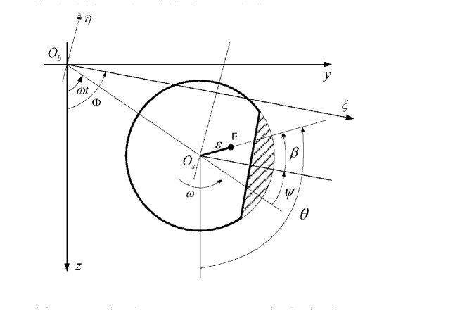
Figure 1: Schematic plot of the cracked Jeffcott rotor [7].

Tondl [9], Cohen and Porat [10] and Bernasconi [11] showed that typical lateral excitations, such as unbalance, may result in both lateral and torsional responses of uncracked rotor. Continuing these works Muszynska et al. [12] and Bently et al. [13] discussed rotor coupled lateral and torsional vibrations due to unbalance. Their experimental results exhibited the existence of significant torsional vibrations, due to coupling with the lateral modes. Further reported works have used this coupling under external excitation as a means to identify the presence of cracks [14, 15]. It has become clear that the spectral components of the shaft response under radial excitation can be used to identify the presence of transverse shaft cracks. In particular, Iwatsubo et al. [16] considered the vibrations of a slowly rotating shaft subject to either periodic or impulsive excitation. They identified specific harmonics in the response spectrum, which are combinations between the rotation speed and excitation frequency and they can be used to detect the presence of the crack. Also, Iwatsubo et al. [16] noted that the sensitivity of the response to the magnitude of the damage depends on the value of the excitation frequency chosen for the detection. Finally, Ishida and Inoue [17] considered the response of a horizontal rotor to harmonic external torques. Furthermore, Sawicki et al. [18, 19, 7] examined transient response of the cracked rotor, including the stalling effect under the constant driving torque.

In this paper we continue these investigations. By applying the external harmonic torque excitation we show the characteristic features of internal resonances leading to quasi-periodic and non–periodic types of motion.

2 The model and equations of motion

The model of the Jeffcott rotor, which is by a definition limited to a rotating mass disc and massless rotating elastic shaft, is presented in Fig. 1.

The angular position of the unbalance vector can be written as

$$\theta(t)=\omega t+\psi(t)+\beta,$$ (1)

where $\omega$ is a constant spin speed of the shaft, $\psi(t)$ is a torsional angle, while $\beta$ is the fixed angle between the unbalance vector and the centerline of the transverse shaft surface crack. It should be noted that

$$\dot{\theta}=\dot{\Phi}=\omega+\dot{\psi},\hskip 28.45274pt\ddot{\theta}=\ddot{\psi},$$ (2)

where $\Phi$ is the spin angle of the rotor (Fig. 1).

The kinetic $T$ and potential $U$ energies for the rotor system subjected to lateral and torsional vibrations can be expressed as follows:

$$T=\frac{1}{2}J_{p}\dot{\theta}^{2}+\frac{1}{2}M\left(\dot{z}^{2}+\dot{y}^{2}\right)+\frac{1}{2}M\epsilon^{2}\dot{\theta}^{2}+M\epsilon\dot{\theta}\left(-\dot{z}\sin\theta+\dot{y}\cos\theta\right)$$ (3)

$$U=\frac{1}{2}\left\{z~{}y\right\}{\bf K}_{I}\left\{\begin{array}[]{c}z\\ y\end{array}\right\}+\frac{1}{2}k_{t}\psi^{2},$$ (6)

where the stiffness matrix reads

$${\bf K}_{I}=\left[\begin{array}[]{cc}k_{zz}&k_{zy}\\ k_{yz}&k_{yy}\end{array}\right].$$ (9)

The coupled equations for transverse and torsional motion for the rotor system take the following form:

$$M\ddot{z}+C_{l}\dot{z}+k_{zz}z+k_{zy}y=F_{z}+M\epsilon\left(\dot{\theta}^{2}\cos\theta+\ddot{\theta}\sin\theta\right)$$ (10)

$$M\ddot{y}+C_{t}\dot{z}+k_{yz}z+k_{yy}y=F_{y}+M\epsilon\left(\dot{\theta}^{2}\sin\theta+\ddot{\theta}\cos\theta\right)$$ (11)

$$J_{p}\ddot{\psi}+C_{t}\dot{\psi}+\epsilon C_{l}(\dot{z}\sin\theta-\dot{y}\cos\theta)-\epsilon(F_{z}\sin\theta-F_{y}\cos\theta)$$ (12)

$$+\epsilon\left[(k_{zz}z+k_{zy}y)\sin\theta-(k_{yz}z+k_{yy}y)\cos\theta\right]+\frac{\partial U}{\partial\psi}=T_{e},$$

where $M$ and $J_{p}$ is the mass and mass moment of inertia of the disk, while $\epsilon$ is eccentricity of the disk. $F_{z}$ and $F_{y}$ are the external forces (including gravity) in $z$ and $y$ directions, respectively, $C_{l}$ and $C_{t}$ are lateral and torsional damping coefficients, $T_{e}$ is an external torque. In our case

$$F_{z}=-Mg,~{}~{}~{}~{}F_{y}=0,~{}~{}~{}~{}T_{e}=T_{0}\sin(\omega_{e}t).$$ (13)

where $g$ is the gravitational acceleration, $T_{0}$ and $\omega_{e}$ are amplitude and frequency of the external torque, respectively.

The stiffness matrix for a Jeffcott rotor with a cracked shaft in rotating coordinates can be written as:

$${\bf K}_{R}=\left(\begin{array}[]{cc}k_{\xi}&0\\ 0&k_{\eta}\end{array}\right)=\left(\begin{array}[]{cc}k&0\\ 0&k\end{array}\right)-f(\Phi)\left(\begin{array}[]{cc}\Delta k_{\xi}&0\\ 0&\Delta k_{\eta}\end{array}\right),$$ (20)

where the first matrix, on the left hand side, refers to the stiffness of the uncracked shaft, and the second defines the variations in shaft stiffness $k_{\xi}$ and $k_{\eta}$ in $\xi$ and $\eta$ directions, respectively. The function $f(\Phi)$ is a crack steering function which depends on the angular position of the crack $\Phi$. The hinge model of the crack might be an appropriate representation for very small cracks, Mayes and Davies [20] proposed a model with a smooth transition between the opening and closing of the crack that is more adequate for larger cracks. In this case the crack steering function, or the Mayes function, takes the following form:

$$f(\Phi)=\frac{1+\cos(\Phi)}{2}.$$ (21)

The stiffness matrix for a Jeffcott rotor with a cracked shaft in inertial coordinates, ${\bf K}_{I}$ is derived as

$${\bf K}_{I}={\bf T}{\bf K}_{R}{\bf T}^{-1},~{}~{}~{}{\bf T}=\left(\begin{array}[]{cc}\cos\Phi&-\sin\Phi\\ \sin\Phi&\cos\Phi\end{array}\right),$$ (24)

where

$$\Delta k_{1}=\frac{\Delta k_{\xi}+\Delta_{\eta}}{2},~{}~{}~{}~{}~{}\Delta k_{1}=\frac{\Delta k_{\xi}-\Delta_{\eta}}{2}.$$ (25)

Consequently after [7]:

$$\frac{\partial U}{\partial\psi}=-\frac{k}{4}\frac{\partial f(\Phi)}{\partial\psi}\left[(\Delta k_{1}+\Delta k_{2}\cos 2\Phi)z^{2}\right.$$

$$\left.+2zy\Delta k_{2}\sin 2\Phi+(\Delta k_{1}-\Delta k_{2}\cos 2\Phi)y^{2}\right]$$ (26)

$$+\frac{f(\Phi)k\Delta k_{2}}{2}\left[z^{2}\sin 2\Phi-2zy\cos 2\Phi-y^{2}\sin 2\Phi\right]+k_{t}\psi.$$

3 Results of Simulations

Assuming the example of simply supported steel shaft, with a disc at the center and a transverse crack located near the disk, we applied Eqs. 10-12 and performed the simulations. The parameters of the examined system are shown in the Table 1. Simulations were done using the Euler integration procedure with a integration step $\delta t=2\pi/(36000\omega)$ and a sampling time $\Delta t=1000\delta t$.

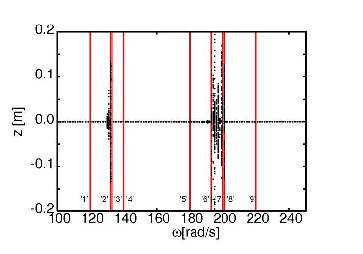
Figure 2: Bifurcation diagram of the cracked rotor. The numbers ’1’–’9’ correspond to $\omega=$ 120, 132, 133, 140, 180, 193, 200, 201, and 220 rad/s.

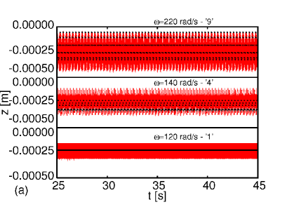
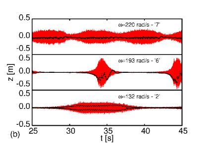
Figure 3: Time histories of displacement in the vertical direction (a) for $\omega=120$, 140, 220 rad/s (small amplitude periodic vibrations) and (b) for $\omega=132$, 200, 201 rad/s (intermittent vibrations). Black points shows stroboscopic points. Numbers ’1’, ’4’, ’9’, ’2’, ’6’, and ’7’ indicate the corresponding values in the bifurcation diagram (Fig. 2).

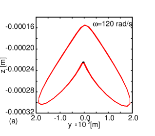
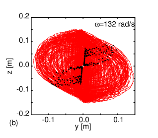
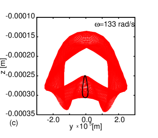
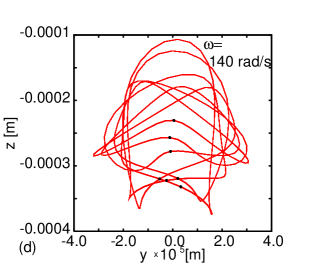
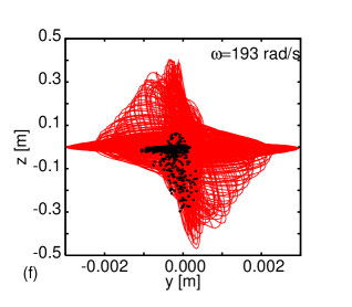
Figure 4: Phase diagram projections into z-y plane for few values of speed velocities ($\omega=120$, 132, 133, 140, 180, 193, 200, and 201).

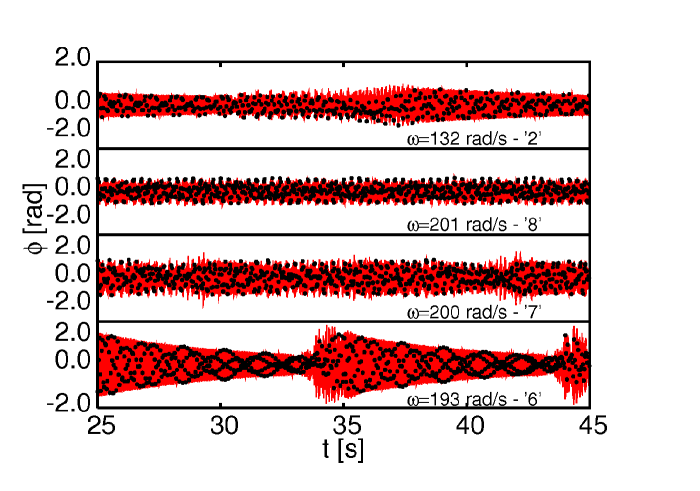
Figure 5: Time histories of torsional angular displacements $\phi$ for intermittent oscillations ($\omega=132$, 193, 200, 201). Black points shows stroboscopic points. Numbers ’6’, ’7’, ’8’, ’2’ indicate the corresponding values in the bifurcation diagram (Fig. 1).

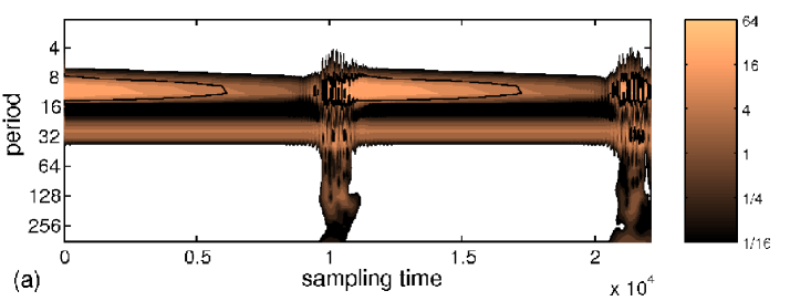
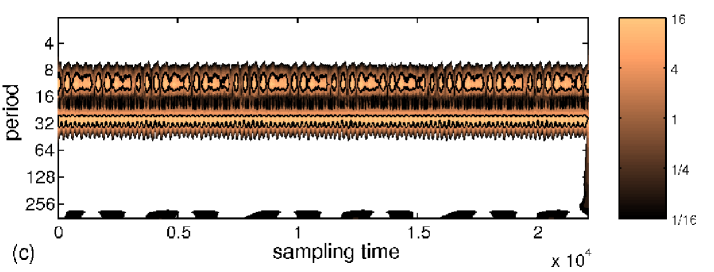
Figure 6: Wavelet power spectra for torsional angular displacements $\phi$; $\omega=193$, 200, 201, 132 for (a), (b), (c), and (d); respectively. Note, the logarithmic colour scale on the right hand side. White regions in figures (a-d) indicate that power spectrum values exceed the scale.

Table 1: Parameters for a simple-supported Jeffcott rotor with a crack.

Disk mass, $M$	3 kg
Disk polar moment of inertia, $J_{p}$	0.01 kg m2
Eccentricity of the disk, $\epsilon$	2.2 $\times$ 10-5 m
Torsional natural frequency, $\omega_{t}$	630 rad/s
Lateral natural frequency, $\omega_{t}$	210 rad/s
Shaft lateral stiffness, $k$	$k=\omega_{l}^{2}M$
Shaft torsional stiffness, $k_{t}$	$k_{t}=\omega_{t}^{2}J_{p}$
Damping ratio in lateral direction, $\xi_{l}$ ($C_{l}=2\xi_{l}M\omega_{l}$)	0.008
Damping ratio in torsional direction, $\xi_{t}$ ($C_{t}=2\xi_{l}J_{p}\omega_{t}$)	0.0006
External torque amplitude, $T_{0}$	800 Nm
External torque amplitude, $\omega_{e}$	$\in[100,250]$ rad/s
Relative stiffness change caused by cracks $\frac{\Delta k_{\xi}}{k}$	0.4
($\Delta k_{1}=\frac{7}{6}\Delta k_{\xi}/k$, $\Delta k_{2}=\frac{5}{6}\frac{\Delta k_{\xi}}{k}$)

The results for the range of rotational velocities $\omega\in[100,250]$ are presented in the bifurcation diagram (Fig. 2). One can see that the resonances appear as they are expected just below the lateral natural frequency and slightly above the half of lateral natural frequency, which one would expect for a non-linear system of this kind. Spanning the rotor spin speed in the range of 145-149 rad/sec and 216-234 rad/sec, reveals the presence of a wide variety of the excited response characteristics. To explain the nature of vibrations in the regions of resonance we focused on the specific frequencies denoted by ’1’–’9’ for the corresponding values $\omega=$ 120, 132, 133, 140, 180, 193, 200, 201, and 220 rad/s. In Fig. 3a we show the time histories of displacement in the vertical direction for nonresonat cases $\omega=$ 120, 140, 220 rad/s. Black points are stroboscopic points plotted with the rotation frequency $\omega$. Note that all three considered here cases indicate periodic vibrations with a small amplitude. On the other hand in Fig. 3b we show the resonant time series with rotation velocities $\omega=$ 132, 200, 201 rad/s. In contrary to the previous cases the displacement $z$ can be large. Interestingly it increases after small laminar behaviour with a relatively small amplitude. Note that in both panels the numbers ’1’, ’4’, ’9’, ’2’, ’6’, and ’7’ indicate the corresponding values $\omega$ in the bifurcation diagram (Fig. 2).

To shed some more light into the lateral modes we plotted, in Figs. 4a-h the phase diagram projections into z-y plane are plotted for few values of speed velocities( $\omega=$ 120, 132, 133, 140, 180, 193, 200, and 201). Black points indicate the corresponding Poincaré maps. In cases of nonresonant vibrations (Figs. 4a,d,e) of small amplitudes we observe with closed lines and a number of singular black points indicating periodic motion. Interestingly in Fig. 4c the Poincare map show a line instead of points indicating the quasiperiodic character of motion. The rest of plots (Fig. 4b,f,g) have non-periodic character. while Fig. 4h has features of moth quasi-periodic and non-periodic. Note that Fig. 4b,f,g, and h look like chaotic attractors, however to tell more about the non-periodic beats nature one should perform standard calculations of Lyapunov exponents or correlation dimension analysis.

Finally in Fig. 5 we plot the time histories of torsional angular displacements ( $\omega=$ 132, 193, 200, 201). Black points shows stroboscopic points. Numbers ’6’, ’7’, ’8’, ’2’ indicate the corresponding values in the bifurcation diagram (Fig. 1). These plots shows the relaxation nature of the torsional oscillations. This is consistent with results for intermittent lateral oscillations presented in Fig. 3. Such an intermittent behaviour can be presented by temporal frequency diagram [22, 23] which can be given by the wavelet power spectra [24]. In Fig. 6 one clearly see the laminar (periodic) interplay with turbulent (chaotic) regions. Note that for smaller rotation velocities we observe longer laminar intervals.

4 Discussion and Conclusions

Using a simple model of the breathing crack we have showed that the response to periodic torque applied at the ends of rotating shaft is complex. In our results we observe on one hand the multi-frequency synchronization, and on the other hand quasi-periodic motion and nonlinear beats in the regions of resonances. Especially the beats are characteristic as far as the nonlinear coupling of lateral and torsional modes induced by the crack is concerned. The beats are visible in both channels. They are also the signatures of interplay of external and parametric excitations, which arise from the crack existence. Interestingly the beats causing the intermittency of the laminar phases introduce the non-periodic element of vibrations. The chaotic nature of such dynamic response of the rotor system exceeds the present report and will be discussed in detail in a future publication.

References

- [1] Gasch R. Dynamic behavior of a simple rotor with a cross-sectional crack. In: Vibrations in Rotating Machinery. The Institution of Mechanical Engineers. Paper C178/76: 123–8; 1976.
- [2] Gasch R. A survey of the dynamic behavior of a simple rotating shaft with a transverse crack. Journal of Sound and Vibration 160: 313–32; 1993.
- [3] Dimarogonas AD. Vibration of cracked structures: a state of the art review. Engineering Fracture Mechanics 55: 831–57; 1996.
- [4] Wauer J. Dynamics of cracked rotors: a literature review. Applied Mechanics Reviews 43 (1) (1990) 13–8.
- [5] Plaut RH, Wauer J. Parametric, external, and combination resonances in coupled flexural and torsional oscillations of an unbalanced rotating shaft. Journal of Sound and Vibration 183; 889–97; 1995.
- [6] Chondros TG, Dimarogonas AD. A consistent cracked bar vibration theory. Journal of Sound and Vibration 200: 303–13; 1997.
- [7] Sawicki JT, Wu X, Gyekenyesi AL, and Baaklini G. Application of nonlinear dynamics tools for diagnosis of cracked rotor vibration signatures. Proc. of SPIE’s Int. Symposium on Smart Structures and Materials, San Diego, California; 2005.
- [8] Penny JET, and Friswell MI. Simplified modelling of rotor cracks. Proc. of ISMA 27, Leuven, Belgium, 607–15; 2002.
- [9] Tondl A. Some Problems of Rotor Dynamics. Publishing House of Czechoslovakia Academy of Science, Prague; 1965.
- [10] Cohen R, Porat I. Coupled torsional and transverse vibration of unbalanced rotor. ASME Journal of Applied Mechanics 52: 701–5; 1985.
- [11] Bernasconi O. Bisynchronous torsional vibrations in rotating shafts. ASME Journal of Applied Mechanics 54: 893–7; 1987.
- [12] Muszynska A, Goldman P, and Bently DE. Torsional/lateral cross-coupled responses due to shafts anisotropy: A new tool in shaft crack detection”, Proc. of IMechE Vibrations in Rotating Machinery C432-090, 257–62; 1992.
- [13] Bently DE, Goldman P, and Muszynska A. ”Snapping” torsional response of an anisotropic radially loaded rotor. Journal of Engineering for Gas Turbines and Power 119: 397–403; 1997.
- [14] Collins KR, Plaut RH, and Wauer J. Detection of cracks in rotating Timoshenko beams using axial impluses. Journal of Vibration and Acoustics 113: 74–8;1991.
- [15] Darpe AK, Gupta K, Chawla A. Coupled bending, longitudinal and torsional vibrations of a cracked rotor. Journal of Sound and Vibration 269: 33–60; 2004.
- [16] Iwatsubo T, Arii S, and Oks A. Detection of a transverse crack in a rotor shaft by adding external force. Proc. IMechE Vibrations in Rotating Machinery, C432/093: 275-282; 1992.
- [17] Ishida Y, Inoue T. Detection of a rotor crack by a periodic excitation. In: Proc. of ISCORMA; 1004–11; 2001.
- [18] Sawicki JT, Wu X, Baaklini G, and Gyekenyesi AL. Vibration-based crack diagnosis in rotating shafts during acceleration through resonance,” Proc. of SPIE 10th Annual International Symposium on Smart Structures and Materials, San Diego, California; 2003.
- [19] Sawicki JT, Bently DE, Wu X, Baaklini G, and Friswell MI. Dynamic behavior of cracked flexible rotor subjected to constant driving torque. Proc. of the 2nd International Symposium on Stability Control of Rotating Machinery, Gdansk, Poland: 231–41; 2003.
- [20] Mayes IW, Davies WGR. Analysis of the response of a multi-rotor-bearing system containing a transverse crack in a rotor. ASME Journal of Vibration, Acoustics, Stress, and Reliability in Design 106: 139–45; 1984.
- [21] Sawicki JT. Some advances in diagnostics of rotating machinery malfunctions. Proc. of the Int. Symposium on Machine Condition Monitoring and Diagnosis, The University of Tokyo, Tokyo: 138–43; 2002.
- [22] Sen AK, Litak G, and Syta A. Cutting process dynamics by nonlinear time series and wavelet analysis. Chaos 17: 023133; 2007.
- [23] Sen AK, Litak G, Taccani R, and Radu R. Wavelet analysis of cycle-to-cycle pressure variations in an internal combustion engine. Chaos, Solitons & Fractals, in press, doi:10.1016/j.chaos.2007.01.041
- [24] Torrence C, Compo GP. A practical guide to wavelet analysis. Bulletin of the American Meteorological Society 79; 61–78; 1998.