Spatiotemporal correlations in entangled photons
generated by spontaneous parametric down conversion

Abstract

In most configurations aimed at generating entangled photons based on spontaneous parametric down conversion (SPDC), the generated pairs of photons are required to be entangled in only one degree of freedom. Any distinguishing information coming from the other degrees of freedom that characterize the photon should be suppressed to avoid correlations with the degree of freedom of interest. However, this suppression is not always possible. Here, we show how the frequency information available affects the purity of the two-photon state in space, revealing a correlation between the frequency and the space degrees of freedom. This correlation should be taken into account to calculate the total amount of entanglement between the photons.

1 Introduction

Pairs of photons generated via spontaneous parametric down conversion (SPDC) are widely used in quantum cryptography, to test violation of Bell’s inequalities and in other quantum information tasks, including dense coding and teleportation [1]. The popularity of this source of paired photons is strongly related to the relative simplicity of its experimental realization, and to the variety of quantum features that down converted photons can exhibit. It is well known that a pair of photons generated via SPDC can be entangled in different degrees of freedom, for example in polarization [2, 3], in frequency [4, 5] and in the equivalent degrees of freedom: orbital angular momentum [6, 7], space and transverse momentum [8, 9].

Usually, when considering entanglement between the two generated photons, only one of the degrees of freedom in which the pair may be entangled is considered and any influence of the others is neglected. This is often justified by the assumption of a filtering process in which the use of very narrow filters in one degree of freedom allows to neglect it [10]. Only one degree of freedom is considered, for example, in the experimental demonstration of teleportation [11] and in some proposals to measure the spatial entanglement between paired photons [8].

Pairs of photons generated with specific characteristics in various degrees of freedom have been also considered. For example, in hyperentanglement [12, 13] where the photons are entangled in various degrees of freedom that are assumed to be independent and, in configurations where one degree of freedom modifies the quantum state of the photons in other degrees of freedom: to distillate position entanglement using the polarization [14] or to control the joint frequency distribution of the generated pair by modifying the spatial properties of the pump beam [5].

All the configurations mentioned before assume a specific relationship between frequency, polarization and space in the two-photon state. In this paper, we will concentrate on the frequency and spatial properties of a pure two-photon state. We will show that the purity of the spatial two-photon state generated by SPDC depends on the frequency information available. This imply a correlation between space and frequency that cannot be ignored in any real filtering process, where the finite bandwidth of the filters affects the separability of the frequency and the space degrees of freedom. This is analogous to the effect of the spatial [15] and frequency [16] correlations of the paired photons on the degree of polarization entanglement of the generated photons. Additionally, in this letter we will show how the spatiotemporal correlations affect the entanglement between the photon. We will calculate how the purity of the signal photon in space and frequency, and therefore the amount of entanglement between the photons, depends on the geometry of the SPDC configuration, the characteristics of the pump beam and the filtering process.

This paper is divided in three sections. In section 2 we discuss the main characteristics of the two-photon quantum state generated in spontaneous parametric down conversion considering the space and frequency degrees of freedom. In section 3, the spatial state of the two-photon is described. It is shown how the spatial state may become mixed as a consequence of tracing out the frequency variables, which implies correlation between those degrees of freedom. Finally, in section 4, the purity of the signal photon state is analyzed taking into account the space and the frequency degrees of freedom.

2 Quantum State of pairs of photons generated via spontaneous parametric down conversion

2.1 General case

Spontaneous parametric down conversion (SPDC) is an optical process in which a nonlinear crystal of length $L$ is illuminated by a laser pump beam propagating in the $z$ direction. Due to the interaction of a pump photon with the crystal there is a small probability to generate a pair of photons: signal and idler. In general, the direction of propagation of the pump beam is modified by a small angle $\rho_{0}$ due to the presence of Poynting vector walk-off inside the crystal. All photons that interacts in the nonlinear process are characterized by the transverse momentum $\mathbf{q_{n}}=(q_{n}^{x},q_{n}^{y})$, and the frecuency $\omega_{n}=\omega_{n}^{0}+\Omega_{n}$, where $\omega_{n}^{0}$ is the central frequency and $\Omega_{n}$ is the frequency deviation. The index $n$ labels the signal $(n=s)$, idler $(n=i)$ and pump $(n=p)$.

For the sake of simplicity, in what follows we will assume that in the frequency and space degrees of freedom, the two-photon state is pure [17], therefore the density matrix reads

$$\rho= \int d\mathbf{q}_{s}d\Omega_{s}d\mathbf{q}_{i}d\Omega_{i}d\mathbf{q}_{s}^{\prime}d\Omega_{s}^{\prime}d\mathbf{q}_{i}^{\prime}d\Omega_{i}^{\prime}$$

$$\times\Phi(\mathbf{q}_{s},\Omega_{s},\mathbf{q}_{i},\Omega_{i})\Phi^{*}(\mathbf{q}^{\prime}_{s},\Omega^{\prime}_{s},\mathbf{q}^{\prime}_{i},\Omega^{\prime}_{i})$$

$$\times|\mathbf{q}_{s},\Omega_{s}\rangle|\mathbf{q}_{i},\Omega_{i}\rangle\langle\mathbf{q}^{\prime}_{s},\Omega^{\prime}_{s}|\langle\mathbf{q}^{\prime}_{i},\Omega^{\prime}_{i}|.$$

The spatiotemporal mode function $\Phi(\mathbf{q}_{s},\Omega_{s},\mathbf{q}_{i},\Omega_{i})$ in a noncollinear configuration is given by

$$\Phi(\mathbf{q}_{s},\Omega_{s},\mathbf{q}_{i},\Omega_{i}) \propto E_{p}(q_{s}^{x}+q_{i}^{x},\Delta_{0})B_{p}(\Omega_{s}+\Omega_{i})$$

$$\times\mathcal{C}_{spatial}(\mathbf{q}_{s})\mathcal{C}_{spatial}(\mathbf{q}_{i})$$

$$\times\mathcal{F}_{frequency}(\Omega_{s})\mathcal{F}_{frequency}(\Omega_{i})$$

$$\times\mathrm{sinc}\left(\frac{\Delta_{k}L}{2}\right)$$

where $B_{p}(\omega_{p}^{0}+\Omega_{p})$ and $E_{p}(\mathbf{q}_{p})$ are the frequency and transverse momentum distribution of the pump beam at the center of the nonlinear crystal, respectively. The effect of the unavoidable spatial filtering produced by the specific optical detection system is described by the spatial collection function $\mathcal{C}_{spatial}(\mathbf{q}_{n})$. The presence of frequency filters in the paths of signal and idler is indicated by frequency filter function $\mathcal{F}_{frequency}(\Omega_{n})$. The Phase matching conditions appears in equation (2.1) through the “Delta” factors, defined by

$$\Delta_{0} = q_{s}^{y}\cos\varphi_{s}+q_{i}^{y}\cos\varphi_{i}+k_{s}\sin\varphi_{s}-k_{i}\sin\varphi_{i}$$ (3)

$$\Delta_{k} = k_{p}-k_{s}\cos\varphi_{s}-k_{i}\cos\varphi_{i}-q_{s}^{y}\sin\varphi_{s}+q_{i}^{y}\sin\varphi_{i}$$

$$+(q_{s}^{x}+q_{i}^{x})\tan\rho_{0}\cos\alpha+\Delta_{0}\tan\rho_{0}\sin\alpha$$

where $k_{n}=\left[\left(\omega_{n}^{0}n_{n}/c\right)^{2}-|\mathbf{q}_{n}|^{2}\right]^{1/2}$ is the longitudinal wave vector inside the crystal. $\varphi_{s}$ and $\varphi_{i}$ are the propagation directions of the generated photons inside the crystal with respect to the pump direction $z$ and $\alpha$ is the azimuthal angle [10, 18].

2.2 Gaussian approximations

In order to find analytical expressions for the purity of the spatial two-photon state and the purity of the signal state in frequency and space, we make some assumptions and approximations following refs [19, 20].

We consider a gaussian shape for the spatial and frequency distributions of the pump beam:

$$E_{p}(q_{p}^{x},q_{p}^{y})=\exp\left[-\frac{\mathrm{w}_{p}^{2}}{4}(q_{p}^{x2}+q_{p}^{y2})\right]$$ (4)

and

$$B_{p}(\Omega_{s}+\Omega_{i})=\exp\left[-\frac{T_{0}^{2}}{4}\Omega_{p}^{2}\right].$$ (5)

The pump beam waist is given by $\mathrm{w}_{p}$ and the pulse temporal duration is $T_{0}$.

Both, the spatial collection and the frequency filter functions are described by Gaussians, so that $\mathcal{C}_{spatial}(\mathbf{q}_{n})\propto\exp\left[-\mathrm{w}_{n}^{2}|\mathbf{q}_{n}|^{2}/2\right]$ and $\mathcal{F}_{frequency}(\Omega_{n})\propto\exp\left[-\Omega_{n}^{2}/(2B_{n}^{2})\right]$ where $\mathrm{w}_{n}$ is the spatial collection mode width and $B_{n}$ is the frequency bandwidth. Notice that, in order to have more convenient units, the filters in momentum are defined in a different way than the filters in frequency. While $B_{s,i}\rightarrow 0$ implies a single frequency collection, the condition for a single q vector collection is $w_{s,i}\rightarrow\infty$. In what follows we consider $B_{s}=B_{i}$ and $\mathrm{w}_{s}=\mathrm{w}_{i}$.

Under these considerations and by making the approximation $\mathrm{sinc}\left(\Delta_{k}L/2\right)\approx\exp\left[-\beta^{2}\Delta_{k}^{2}L^{2}/4\right]$ with $\beta=0.455$, the mode function of the generated pair can be written as

$$\Phi(\mathbf{q}_{s},\Omega_{s},\mathbf{q}_{i},\Omega_{i})=N\exp\left[-\frac{1}{2}x^{t}Ax\right]$$ (6)

where $N$ is a normalization constant, $A$ is a positive-definite real $6\times 6$ matrix containing all the parameters that describes the SPDC process and $x^{t}$ is the transpose of the vector $x$ given by $x^{t}=\left(\begin{array}[]{cccccc}q_{s}^{x},&q_{s}^{y},&\Omega_{s},&q_{i}^{x},&q_{i}^{y},&\Omega_{i}\\ \end{array}\right)$.

The physical system described by equation (6) can be considered as composed by two subsystems. These subsystems can either be the two degrees of freedom, figure 1 (a) or the two photons, figure 1 (b). In both cases, the correlations that may exist between the subsystems imply that the system is not in a separable state, i.e., when considering the two degrees of freedom $\Phi(\mathbf{q}_{s},\Omega_{s},\mathbf{q}_{i},\Omega_{i})\neq\Phi_{\mathbf{q}}(\mathbf{q}_{s},\mathbf{q}_{i})\Phi_{\Omega}(\Omega_{s},\Omega_{i})$ and when considering the two photons $\Phi(\mathbf{q}_{s},\Omega_{s},\mathbf{q}_{i},\Omega_{i})\neq\Phi_{s}(\mathbf{q}_{s},\Omega_{s})\Phi_{i}(\mathbf{q}_{i},\Omega_{i})$.

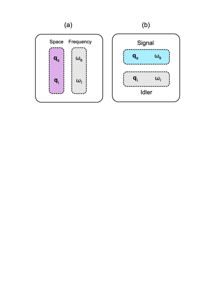
Figure 1: The two-photon state in space and frequency can be considered as composed by two subsystems. In (a) those subsystems are the degrees of freedom. The frequency, in gray, is traced out in the calculations of Sec. 3. In (b) the subsystems considered are the generated photons. In gray we show the idler photon that is traced out in the calculations of Sec. 4.

3 Correlations between space and frequency degrees of freedom

Let us consider the two degrees of freedom as subsystems like in figure  1(a). The state of one subsystem can be calculated tracing out the parameters that describe the other subsystem. Tracing out the frequency, the reduced density matrix for the resulting spatial two-photon state is given by

$$\rho_{\mathbf{q}} = Tr_{\Omega}(\rho)$$

$$= \int d\Omega_{s}^{\prime\prime}d\Omega_{i}^{\prime\prime}\langle\Omega_{s}^{\prime\prime},\Omega_{i}^{\prime\prime}|\rho|\Omega_{s}^{\prime\prime}\Omega_{i}^{\prime\prime}\rangle$$

$$= \int d\mathbf{q}_{s}d\Omega_{s}d\mathbf{q}_{i}d\Omega_{i}d\mathbf{q}_{s}^{\prime}d\mathbf{q}_{i}^{\prime}$$

$$\Phi(\mathbf{q}_{s},\Omega_{s},\mathbf{q}_{i},\Omega_{i})\Phi^{*}(\mathbf{q}^{\prime}_{s},\Omega_{s},\mathbf{q}^{\prime}_{i},\Omega_{i})|\mathbf{q}_{s},\mathbf{q}_{i}\rangle\langle\mathbf{q}^{\prime}_{s},\mathbf{q}^{\prime}_{i}|$$

and the corresponding purity $Tr(\rho_{\mathbf{q}}^{2})$ of the spatial two-photon state is

$$Tr(\rho_{\mathbf{q}}^{2}) =\int d\mathbf{q}_{s}d\Omega_{s}d\mathbf{q}_{i}d\Omega_{i}d\mathbf{q}_{s}^{\prime}d\Omega_{s}^{\prime}d\mathbf{q}_{i}^{\prime}d\Omega_{i}^{\prime}$$

$$\times\Phi(\mathbf{q}_{s},\Omega_{s},\mathbf{q}_{i},\Omega_{i})\Phi^{*}(\mathbf{q}^{\prime}_{s},\Omega_{s},\mathbf{q}_{i}^{\prime},\Omega_{i})$$

$$\times\Phi(\mathbf{q}_{s}^{\prime},\Omega_{s}^{\prime},\mathbf{q}_{i}^{\prime},\Omega_{i}^{\prime})\Phi^{*}(\mathbf{q}_{s},\Omega_{s}^{\prime},\mathbf{q}_{i},\Omega_{i}^{\prime}).$$

We can solve this integral using the exponential character of the mode function given by equation (6), so that the purity becomes

$$Tr(\rho_{\mathbf{q}}^{2})=\frac{\det(2A)}{\sqrt{\det(B)}}$$ (9)

where $B$ is a positive-definite real $12\times 12$ matrix given by

$$N^{4}\exp\left[-\frac{1}{2}X^{t}BX\right]=\Phi(\mathbf{q}_{s},\Omega_{s},\mathbf{q}_{i},\Omega_{i})$$ (10)

$$\times\Phi^{*}(\mathbf{q}^{\prime}_{s},\Omega_{s},\mathbf{q}^{\prime}_{i},\Omega_{i})\Phi(\mathbf{q}_{s}^{\prime},\Omega_{s}^{\prime},\mathbf{q}_{i}^{\prime},\Omega_{i}^{\prime})\Phi^{*}(\mathbf{q}_{s},\Omega_{s}^{\prime},\mathbf{q}_{i},\Omega_{i}^{\prime}).$$

$X^{t}=\left(\begin{array}[]{cc}x^{t},&x^{\prime t}\\ \end{array}\right)$ is a vector resulting from the concatenation of $x^{t}$ and $x^{\prime t}=\left(\begin{array}[]{cccccc}q_{s}^{x^{\prime}},&q_{s}^{y^{\prime}},&\Omega_{s}^{\prime},&q_{i}^{x^{\prime}},&q_{i}^{y^{\prime}},&\Omega^{\prime}_{i}\\ \end{array}\right)$.

Since the composed quantum system described by equation (LABEL:densitymatrix) is in a pure state ($Tr(\rho^{2})=1$), the purity of the spatial two-photon state given by equation 9, is different from $1$ only if the degrees of freedom are correlated [21]. This correlation is stronger when the partial purity gets closer to $0$ [1].

Notice that the purity of the spatial two-photon state is equal to the purity of the frequency two-photon state when the spatial degree of freedom is traced out. Therefore all the results derived for the spatial two-photon state can be extended to a frequency two-photon state.

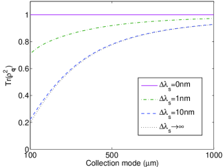
Figure 2: Purity of the spatial state of the pair of generated photons for different values of the frequency filter bandwidth, as a function of the spatial collection mode width ($\mathrm{w}_{s}=\mathrm{w}_{i}$). The pump beam waist is $\mathrm{w}_{p}=400\mu m$ and the emission angle is $\varphi=10^{\circ}$.

We plot the purity of the spatial state $Tr(\rho_{\mathbf{q}}^{2})$ as a function of the spatial filter width for different frequency filter bandwidths, figure  2. The half width at $1/e$ of the frequency filters in the wavelength variable is given by $\Delta\lambda_{n}$, that is related to $B_{s}$ and $B_{i}$ by $B_{n}=\pi c\Delta\lambda_{n}/(\lambda_{n}^{2}\sqrt{\ln 2})$. The SPDC process considered occurs in a $L=1$ mm lithium iodate ($LiIO_{3}$) type I crystal, illuminated by a pump beam with $\lambda_{p}^{0}=405$ nm and a beam waist $\mathrm{w}_{p}=400$ $\mu$m. The generated signal and idler photons are emitted with a wavelength $\lambda_{s}^{0}=\lambda_{i}^{0}=810$ nm at an angle $\varphi=\varphi_{s}=\varphi_{i}=10^{\circ}$. We consider negligible Poynting vector walk-off ($\rho_{0}=0$) and in this case all the values of $\alpha$ are equivalent.

In figure  2 we see that the purity of the spatial two photon state can be different from $1$, which implies a correlation between space and frequency. The strength of the correlation increases as the purity decreases. From this figure we can see that as $\mathrm{w}_{s}$ and $\mathrm{w}_{i}$ increase the spatial purity of the two-photon state gets closer to $1$. This can be understood intuitively since an infinitely big $\mathrm{w}_{s}$ ($\mathrm{w}_{i}$) implies the case of collecting only one $\mathbf{q}_{s}$ ( $\mathbf{q}_{i}$) and therefore the two-photon state is separable in frequency and space.

The separability and the lack of correlation between frequency and space, can also be seen in the “narrow band” limit where $\Delta\lambda_{s}=\Delta\lambda_{i}\rightarrow 0$ nm: for any value of $\mathrm{w}_{s}=\mathrm{w}_{i}$ the purity is always $1$. For a typical commercial interference filter, $\Delta\lambda_{s}=\Delta\lambda_{i}\approx 1$ nm, the correlation between space and frequency is significant and consequently the purity decreases as can be observed in the figure. As the width of the frequency filters increases, the purity converge quickly enough to make the case of $\Delta\lambda_{s}=\Delta\lambda_{i}=10$ nm almost equivalent to the case without frequency filters $\Delta\lambda_{s},\Delta\lambda_{i}\rightarrow\infty$.

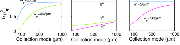
Figure 3: Spatial purity as function of the collection mode for three experimental cases. In (a) is showed the case of reference [5], in (b) the case described in reference [22] and in (c) the case reported in reference [23].

In order to compare these theoretical results with previous works, in figure 3 we show the purity of the spatial state as a function of the collection mode, for three reported experiments. In figure 3 (a) we used the data of reference [5]. In their case, a type I SPDC process in a $1$mm long $LiIO_{3}$ crystal is analyzed. As a pump beam their considered a diode laser with wavelength $\lambda_{p}=405$nm and bandwidth $\Delta\lambda_{p}=0.4$nm. The pairs of photons generated propagate at $\varphi=17^{o}$ and are detected by using monochromators with $\Delta\lambda_{s,i}=0.2$nm. Two cases are depicted, the first one when the pump beam is focalize with a waist of $w_{p}=30\mu$m over the crystal and the second one where the pump beam waist is $w_{p}=462\mu$m. Their main result is the control of the frequency correlations by changing the spatial properties of the pump beam. As the pump beam influence the spatial shape of the generated photons, they report implicitly a correlation between the space and the frequency. For their spatial collection mode $w_{s}=133,48\mu$m it can be seen in the figure that according with our theoretical model the correlation appears.

Figure 3(b) shows $Tr[\rho_{{\bf q}}^{2}]$ for the case described in reference [22]. A continues wave pump beam with $\lambda_{p}=405$nm is used to generate photons with $\lambda_{s,i}=810$nm in a $1.5$mm length BBO crystal. Interference filters of $\Delta\lambda_{s,i}=10$nm are used before the detection. The pump beam waist satisfies the condition $w_{p}>>L$ and the generated photons propagates at $\varphi=0^{o}$. As it can be seen from the plot, the lack of correlation in this case is due to the collinear configuration. Under the conditions reported, but in a non collinear configuration will not be possible to neglect the space and frequency correlations.

Finally in figure 3(c), $Tr[\rho_{{\bf q}}^{2}]$ is plotted in the case described in reference [23]. In their case a pump beam with $\lambda_{p}=351.1$nm is focused with a waist of $w_{p}\approx 20\mu m$ on a $2$mm long BBO crystal. Generated photons at $\lambda_{s,i}=702$nm, propagating at $4^{o}$, are collected after passing $10$nm interference filters. In this noncollinear case, the lack of correlations are due the small pump beam waist. As can be seen in the figure, for less focused pump beams the correlations become appreciable.

4 Spatiotemporal entanglement between signal and idler

The correlations between frequency and space in the two photon states showed in the previous section, suggest that for a complete description of the entanglement between the photons, both degrees of freedom need to be taken into account.

In contrast with the previous section, here the physical system considered is composed of two photons, each one described with space and time variables, like is shown in figure  1 (b). In what follows, we will calculate the purity of the signal photon. Since the global state given by equation (LABEL:densitymatrix) is pure, the result of this section allows us to calculate the degree of spatiotemporal entanglement between signal and idler.

The reduced density matrix in space and frequency for the signal, calculated by making a partial trace over the idler photon, writes

$$\rho_{signal} = Tr_{idler}(\rho)$$

$$= \int d\mathbf{q}_{i}^{\prime\prime}d\Omega_{i}^{\prime\prime}\langle\mathbf{q}_{i}^{\prime\prime},\Omega_{i}^{\prime\prime}|\rho|\mathbf{q}_{i}^{\prime\prime},\Omega_{i}^{\prime\prime}\rangle$$

$$= \int d\mathbf{q}_{s}d\Omega_{s}d\mathbf{q}_{i}d\Omega_{i}d\mathbf{q}_{s}^{\prime}d\Omega_{s}^{\prime}$$

$$\Phi(\mathbf{q}_{s},\Omega_{s},\mathbf{q}_{i},\Omega_{i})\Phi^{*}(\mathbf{q}^{\prime}_{s},\Omega_{s}^{\prime},\mathbf{q}_{i},\Omega_{i})|\mathbf{q}_{s},\Omega_{s}\rangle\langle\mathbf{q}^{\prime}_{s},\Omega_{s}^{\prime}|$$

and its purity is given by

$$Tr(\rho_{signal}^{2}) =\int d\mathbf{q}_{s}d\Omega_{s}d\mathbf{q}_{i}d\Omega_{i}d\mathbf{q}_{s}^{\prime}d\Omega_{s}^{\prime}d\mathbf{q}_{i}^{\prime}d\Omega_{i}^{\prime}$$

$$\times\Phi(\mathbf{q}_{s},\Omega_{s},\mathbf{q}_{i},\Omega_{i})\Phi^{*}(\mathbf{q}^{\prime}_{s},\Omega_{s}^{\prime},\mathbf{q}_{i},\Omega_{i})$$

$$\times\Phi(\mathbf{q}_{s}^{\prime},\Omega_{s}^{\prime},\mathbf{q}_{i}^{\prime},\Omega_{i}^{\prime})\Phi^{*}(\mathbf{q}_{s},\Omega_{s},\mathbf{q}_{i}^{\prime},\Omega_{i}^{\prime}).$$

Recalling the exponential character of the mode function described by equation  (6), we can write equation  (4) as

$$Tr(\rho_{signal}^{2})=\frac{\det(2A)}{\sqrt{\det(C)}},$$ (13)

where $C$ is a positive-definite real $12\times 12$ matrix given by

$$N^{4}\exp\left[-\frac{1}{2}X^{t}CX\right]=\Phi(\mathbf{q}_{s},\Omega_{s},\mathbf{q}_{i},\Omega_{i})$$ (14)

$$\times\Phi^{*}(\mathbf{q}^{\prime}_{s},\Omega_{s}^{\prime},\mathbf{q}_{i},\Omega_{i})\Phi(\mathbf{q}_{s}^{\prime},\Omega_{s}^{\prime},\mathbf{q}_{i}^{\prime},\Omega_{i}^{\prime})\Phi^{*}(\mathbf{q}_{s},\Omega_{s},\mathbf{q}_{i}^{\prime},\Omega_{i}^{\prime}).$$

Notice that the difference between the matrix $C$ and matrix $B$, in the last section, is the order of the primed and unprimed variables in the arguments of the mode function.

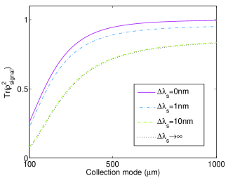
Figure 4: Purity of the spatial frequency state of the signal photon for different values of the frequency filter bandwidth as a function of the spatial collection mode width ($\mathrm{w}_{s}=\mathrm{w}_{i}$). The pump beam waist is $\mathrm{w}_{p}=400\mu m$ and the emission angle is $\varphi=10^{\circ}$.

Figure 4 shows the space-frequency purity of the signal photon as a function of the spatial filter width for different values of the frequency filter width. Maximal separability for the photons is achieved when infinitely narrow filters in space and frequency are used. In the region of small values of $\mathrm{w}_{s}$ and $\mathrm{w}_{i}$, the correlations between frequency and space are considerable even in the case of infinitely narrow frequency filters. Different values for the signal photon purity can be achieved by changing the filters width, as it can be seen from figure 4. It is important to take into account that $Tr(\rho_{signal}^{2})$ is confined between the values obtained for $\Delta\lambda_{s}=\Delta\lambda_{i}\rightarrow 0$ nm and $\Delta\lambda_{s},\Delta\lambda_{i}\rightarrow\infty$. This limits can be tailored by modifying the SPDC configuration. Furthermore, in specific configurations where non infinite filter are used in space and/or frequency, the purity can be tailored by using other parameters.

Figure 5 shows $Tr(\rho_{signal}^{2})$ as a function of the pump beam waist $\mathrm{w}_{p}$ for various values of the emission angle $\varphi=\varphi_{s}=\varphi_{i}$. In figure  5 (a) we considered a frequency filter $\Delta\lambda_{s}=\Delta\lambda_{i}=10$ nm with infinitely narrow spatial filters. In this case, maximal purity can be found for each emission angle at a particular value of the pump beam waist. For a highly narrow band frequency filter with a $\mathrm{w}_{s}=\mathrm{w}_{i}=400$ $\mu$m spatial filter, figure  5 (b) shows how the correlation between the photons is minimal for small pump beams being irrelevant the emission angle, for this particular crystal length. Finally, in figure 5 (c) the case of finite spatial and frequency filters is despicted. As can be seen, the purity of the signal photon is always smaller than one, it increases for noncollinear angles and it has a maximum for a given value of the pump beam waist.

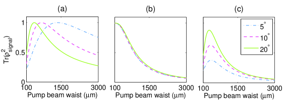
Figure 5: Spatiotemporal purity of the signal photon for different values of the emission angle, as a function of pump beam width ($\mathrm{w}_{p}$). In (a) $\Delta\lambda_{s}=\Delta\lambda_{i}=10$ nm and $\mathrm{w}_{s},\mathrm{w}_{i}\rightarrow\infty$. In (b) $\Delta\lambda_{s},\Delta\lambda_{i}\rightarrow 0$ nm and $\mathrm{w}_{s}=\mathrm{w}_{i}=400$ $\mu$m. In (c) $\Delta\lambda_{s}=\Delta\lambda_{i}=10$ nm and $\mathrm{w}_{s}=\mathrm{w}_{i}=400$ $\mu$m.

From the purity, equation (13), the amount of entanglement between the signal and idler photons can be calculated by using, for example, the I-concurrence $C=\sqrt{2(1-Tr(\rho_{signal}^{2}))}$ [8, 24] or the Schmidt number $K=1/Tr(\rho_{signal}^{2})$ [15].

5 Conclusion

An analytical expression that fully characterizes the purity of the spatial two-photon state was obtained as a function of the parameters involved in the SPDC process, equation (9). The fact that the spatial two-photon state may be mixed reveals a correlation between space and frequency that cannot be neglected even in the cases of very narrow filtering. This results were compared to previous analysis where the correlations between space and frequency are neglected [22, 23] and with other one in witch the correlations appears [5]. This correlation is mathematically analogous to the entanglement in the sense that the mode function $\Phi(\mathbf{q}_{s},\Omega_{s},\mathbf{q}_{i},\Omega_{i})\neq\Phi_{\mathbf{q}}(\mathbf{q}_{s},\mathbf{q}_{i})\Phi_{\Omega}(\Omega_{s},\Omega_{i})$. However, the concept of entanglement is strongly associated to the possibility of a spatial separation of the correlated subsystems.

The purity of the signal photon in space and frequency has been also calculated, equation (13). This expression represents a tool to tailor the space and frequency purity of the signal photon by means of the geometrical SPDC configuration and the filtering process.

References

References

• [1] Nielsen M A and Chuang I L 2000 Quantum Computation and Quantum Information (Cambridge: Cambridge University Press)
• [2] Walborn S P, Padua S and Monken C H 2003 Phys. Rev. A 68 042313
• [3] Kwiat P G, Eberhard P H, Steinberg A M and Chiao R Y 1994 Phys. Rev. A 49 3209
• [4] Mosley P J, Lundeen J S, Smith B J, Wasylczyk P, URen A B, Silberhorn C and Walmsley I A 2008 Phys. Rev. Lett. 100 133601
• [5] Valencia A, Cere A, Shi X, Molina-Terriza G and Torres J P 2007 Phys. Rev. Lett. 99 243601
• [6] Mair A, Vaziri A, Weihs G and Zeilinger A 2001 Nature 412 313
• [7] Molina-Terriza G, Torres J P and Torner L 2007 Nature Phys. 3 305
• [8] Walborn S P and Monken C H 2007 Phys. Rev. A 76 062305
• [9] Law C K and Eberly J H 2004 Phys. Rev. Lett. 92 127903
• [10] Osorio C I, Molina-Terriza G, Font B and Torres J P 2007 Opt. Express 15 14636
• [11] Bouwmeester D, Pan J W, Mattle K, Eibl M, Weinfurter H and Zeilinger A 1997 Nature 390 575
• [12] Barreiro J T, Langford N K, Peters N A and Kwiat P G 2005 Phys. Rev. Lett. 95 260501
• [13] Barbieri M, Cinelli C, Mataloni P and De Martini F 2005 Phys. Rev. A 72 052110
• [14] Caetano D P and Souto Ribeiro P H 2002 Opt. Comm. 211 265
• [15] van Exter M P, Aiello A, Oemrawsingh S S R, Nienhuis G and Woerdmann J P 2006 Phys. Rev. A 74 012309
• [16] Humble T S and Grice W P 2008 Phys. Rev. A 77 022312
• [17] Molina-Terriza G, Vaziri A, Rehacek J, Hradil Z and Zeilinger A 2004 Phys. Rev. Lett. 92 167903
• [18] Torres J P, Molina-Terriza G and Torner L 2005 J. Opt. B: Quantum Semiclass. Opt. 7 235
• [19] Joobeur A, Saleh B E A, Larchuk T S and Teich M C 1996 Phys. Rev. A 53 4360
• [20] Torres J P, Osorio C I and Torner L 2004 Opt. Lett. 29 1939
• [21] Nielsen M A and Kempe J 2001 Phys. Rev. Lett 86 5184
• [22] Yarnall T, Abouraddy A F, Saleh B E A and Teich M C 2008 Opt. Express 16 7634
• [23] Altman A R, Koprulu K G, Corndorf E, Kumar P and Barbosa G A 2005 Phys. Rev. Lett. 94 123601
• [24] Mintert F, Kus M and Buchleitner A 2005 Phys. Rev. Lett. 95 260502