A 610-MHz survey of the Lockman Hole with the Giant Metrewave Radio Telescope – I. Observations, data reduction and source catalogue for the central 5 deg²

Abstract

We present observations of the Lockman Hole taken at 610 MHz with the Giant Metrewave Radio Telescope (GMRT). Twelve pointings were observed, covering a total area of $\sim$5 deg² with a resolution of 6 $\times$ 5 arcsec², position angle $+45\degr$. The majority of the pointings have an rms noise of $\sim$60 $\mu$Jy beam^-1 before correction for the attenuation of the GMRT primary beam. Techniques used for data reduction and production of a mosaicked image of the region are described, and the final mosaic is presented, along with a catalogue of 2845 sources detected above $6\sigma$. Radio source counts are calculated at 610 MHz and combined with existing 1.4-GHz source counts, in order to show that pure luminosity evolution of the local radio luminosity functions for active galactic nuclei and starburst galaxies is sufficient to account for the two source counts simultaneously.

1 Introduction

The Lockman Hole (Lockman, Jahoda & McCammon, 1986) is the region of lowest Hi column density in the sky, with the low infrared background (0.38 MJy sr^-1 at 100 $\mu$m; Lonsdale et al., 2003) making this region particularly well suited for deep infrared observations. The Spitzer Space Telescope (Werner et al., 2004) observed $\sim$12 deg² of the region in 2004 as part of the Spitzer Wide-area Infrared Extragalactic survey (SWIRE; Lonsdale et al., 2003). Observations were centered on $10^{\rm h}45^{\rm m}00^{\rm s}$, $+58\degr 00^{\prime}00^{\prime\prime}$ (J2000 coordinates, which are used throughout this work) using the Infrared Array Camera (IRAC; Fazio et al., 2004) operating at 3.6, 4.5, 5.8 and 8 $\mu$m, and the Multiband Imaging Photometer for Spitzer (MIPS; Reike et al., 2004) at 24, 70 and 160 $\mu$m.

A great deal of complementary data has been taken on the Lockman Hole at other wavelengths in order to exploit the availability of sensitive infrared observations. There have been deep optical observations in the $U$, $g^{\prime}$, $r^{\prime}$ and $i^{\prime}$ bands taken with the Mosaic-I camera at Kitt Peak National Observatory (KPNO), to $5\sigma$ Vega magnitude limits of 24.1, 25.1, 24.4 and 23.7 respectively (Surace et al., 2005). There is existing near-infrared data across the region from the Two Micron All Sky Survey (2MASS; Beichman et al., 2003), to $J$, $H$ and $K_{\rm s}$ band magnitudes of 17.8, 16.5 and 16.0, and a band-merged catalogue containing 323 044 sources from the IRAC, MIPS 24 $\mu$m, 2MASS and KPNO data has been produced (Surace et al., 2005). A photometric redshift catalogue containing 229 238 galaxies and quasars within the Lockman Hole has been constructed from the band-merged data (Rowan-Robinson et al., 2008). Data Release Six of the Sloan Digital Sky Survey (SDSS DR6; Adelman-McCarty et al., 2007) covers the whole region in the $ugriz$ bands, with both photometric and spectroscopic observations available to a depth of $\sim$22 mag. Further deep infrared observations of the Lockman Hole are underway as part of the Deep Extragalactic Survey section of the UK Infrared Deep Sky Survey (UKIDSS; Lawrence et al., 2007) in the $J$, $H$ and $K$ bands, with a target sensitivity of $J\sim 22$ mag. There have been deep surveys of the Lockman Hole with the Submillimetre Common-User Bolometer Array (SCUBA; Holland et al., 1999) at 850 $\mu$m (Coppin et al., 2006), and with the X-ray satellites ROSAT (Hasinger et al., 1998), XMM-Newton (Hasinger et al., 2001; Mainieri et al., 2002; Brunner et al., 2008) and Chandra (Polletta et al., 2006).

A variety of radio surveys cover areas within the Lockman Hole. The first of these was by de Ruiter et al. (1997), who observed 149 1.4-GHz sources within an area of 0.35 deg², using the Very Large Array (VLA) in C-configuration, with an rms noise level of 30-55 $\mu$Jy beam^-1. A similar deep observation was carried out by Ciliegi et al. (2003), who observed 63 sources at 4.9 GHz within a 0.087 deg² region, using the VLA in C-configuration, with an rms noise level of 11 $\mu$Jy beam^-1. More recently, Biggs & Ivison (2006) found 506 sources within a 0.35 deg² area, using the VLA at 1.4 GHz operating in the A- and B-configurations, and with an rms noise level of 4.6 $\mu$Jy beam^-1. The Faint Images of the Radio Sky at Twenty-cm (FIRST; Becker, White & Helfand, 1995) and NRAO VLA Sky Survey (NVSS; Condon et al., 1998) surveys both cover the entire region at 1.4 GHz, but only to relatively shallow noise levels of 150 and 450 $\mu$Jy beam^-1 respectively.

There is a clear need for deep radio observations over a significant area within the Lockman Hole, in order to extend the multi-wavelength information presently available for a large number of sources. In this paper, we present observations of the Lockman Hole taken at 610 MHz with the Giant Metrewave Radio Telescope (GMRT; Ananthakrishnan, 2005), covering $\sim$5 deg² of sky with a resolution of $6\times 5$ arcsec², position angle (PA) $+45\degr$ and centred on $10^{\rm h}45^{\rm m}00^{\rm s}$, $+58\degr 00^{\prime}00^{\prime\prime}$ to match the SWIRE coverage. This is the third in a series of 610-MHz GMRT surveys targeting the Spitzer deep legacy survey regions, following the Spitzer extragalactic First Look Survey (xFLS; Garn et al., 2007) and the European Large Area ISO Survey-North 1 (ELAIS-N1) survey (EN1; Garn et al., 2008). This work, in combination with the deep optical and infrared data, will be used to study the infrared / radio correlation for star-forming galaxies (e.g. Helou, Soifer & Rowan-Robinson, 1985; Condon, 1992; Garrett, 2002; Appleton et al.,, 2004; Murphy et al.,, 2006; Vlahakis, Eales & Dunne, 2007; Ibar et al.,, 2008; Garn, Ford & Alexander, 2008), and the link between star formation and Active Galactic Nuclei (AGN) activity (e.g. Richards et al., 2007; Bundy et al., 2007), as well as the properties of the faint radio source population at 610 MHz (Bondi et al., 2007; Moss et al., 2007; Tasse et al., 2007; Garn et al., 2008).

In Section 2 we describe the observations and data reduction techniques used in the creation of the survey. Section 3 presents the mosaic and a source catalogue containing 2845 sources above $6\sigma$. In Section 4 we calculate the 610-MHz differential source counts, and using local radio luminosity functions obtained from the literature, we demonstrate that a model of pure luminosity evolution is sufficient to account for the differential source counts at 610 MHz and 1.4 GHz simultaneously.

Throughout this work a flat cosmology with $\Omega_{\Lambda}=0.7$ and $H_{0}=70$ km s^-1 Mpc^-1 is assumed.

2 Observations and data reduction

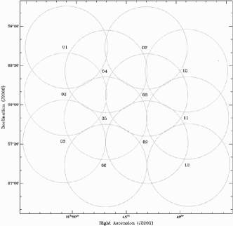
Figure 1: The arrangement of 12 pointings observed in the central region of the Lockman Hole.

The ‘central’ region of the Lockman Hole, consisting of 12 pointings spaced by 36 arcmin in a hexagonal pattern (shown in Fig. 1) was observed in 2004 July 24 and 25, using the GMRT operating at 610 MHz. A further 26 pointings surrounding the central region (the ‘outer’ region) were observed in 2006 July in order to complete the coverage of the majority of the region observed by Spitzer. The outer observations suffered from a series of power failures in one of the arms of the GMRT, and required several catch-up observing sessions to cover the whole field. This paper describes the observations of the central 12 pointings only, with the results from the outer region to be presented in Paper II.

The flux density scale was set through observations of 3C48 or 3C286 at the beginning and end of each observing session. The task setjy was used to calculate 610-MHz flux densities of 29.4 and 21.1 Jy respectively, using the Astronomical Image Processing Software (aips) implementation of the Baars et al. (1977) scale. Each field was observed for a series of interleaved scans, varying between 8 and 10 min in duration, in order to maximise the $uv$ coverage. The scans took place over a total time period of 7 and 9 hours on the two days, with the typical total time being spent on each field being 48 min. A nearby phase calibrator, J1035$+$564, was observed for 4 min between every three scans to monitor any time-dependent phase and amplitude fluctuations of the telescope. The measured phase typically varied by less than $10\degr$ between phase calibrator observations.

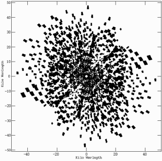
Figure 2: The $uv$ coverage for pointing 10. Baselines less than 1 k$\lambda$ were not used in imaging and have been omitted from the figure.

Observations were made in two 16-MHz sidebands centred on 610 MHz, each split into 128 spectral channels, with a 16.9 s integration time. An error in the timestamps of the uv data was corrected using uvfxt (Garn et al., 2007, for further details see). Initial editing of the data was performed separately on each sideband with standard aips tasks, to remove bad baselines, antennas, and channels that were suffering from large amounts of narrow band interference, along with the first and last integration periods of each scan. The flux calibrators were used to create a bandpass correction for each antenna. In order to create a continuum channel, five central frequency channels were combined together, and an antenna-based phase and amplitude calibration created using observations of J1035$+$564. This calibration was applied to the original data, which was then compressed into 11 channels of bandwidth 1.25 MHz, each small enough that bandwidth smearing was not a problem for our images. The first and last few spectral channels, which tended to be the noisiest, were omitted from the data, leading to an total effective bandwidth of 13.75 MHz in each sideband. Further flagging was performed on the 11-channel data set, and the two sidebands combined using uvflp (again, see Garn et al., 2007) to improve the $uv$ coverage. The $uv$ coverage for one of the pointings is shown in Fig. 2. Baselines shorter than 1 k$\lambda$ were omitted from the imaging, since the GMRT has a large number of small baselines which would otherwise dominate the beam shape.

Each pointing was divided into 31 smaller facets, arranged in a hexagonal grid, which were imaged individually with a separate assumed phase centre. The large total area imaged (a diameter of $1\aas@@fstack{\circ}8$, compared with the full width at half-maximum of the GMRT, which is $\sim$0$\aas@@fstack{\circ}74$) allows bright sources well away from the observed phase centre to be cleaned from the images, while the faceting procedure avoids phase errors being introduced due to the non-planar nature of the sky. All images were made with an elliptical restoring beam of size $6\times 5$ arcsec², PA $+45\degr$, with a pixel size of 1.5 arcsec to ensure that the beam was well oversampled.

The images went through three iterations of phase self-calibration at 10, 3 and 1 min intervals, and then a final iteration of phase and amplitude self-calibration, at 10 min intervals, with the overall amplitude gain held constant in order not to alter the flux density of sources. The self-calibration steps improved the noise level by about 10 per cent, and significantly reduced the residual sidelobes around the brighter sources.

The final rms noise before correction for the GMRT primary beam was between 57 and 63 $\mu$Jy beam^-1 for pointings 1 to 9 and pointing 12, with higher noise levels of around 80 $\mu$Jy beam^-1 for the remaining two pointings. The expected thermal noise limit is $\sim$55 $\mu$Jy beam^-1, calculated using Equation 1 from Garn et al. (2007). The increased noise level for pointings 10 and 11 is due to a very bright radio source (FIRST J103333.2$+$581502), with 1.4-GHz flux density of $\sim$2 Jy, located $\sim$0$\aas@@fstack{\circ}75$ from the pointing centres. This source lies within the region cleaned during the imaging process, but residual sidelobes remain in our mosaic, and the increased noise level is visible in Fig. 3.

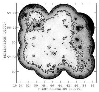
Figure 3: The rms noise of the final mosaic, calculated using SExtractor (see Section 3). The grey-scale ranges between 60 and 300 $\mu$Jy beam^-1, and the contours are at 100 and 200 $\mu$Jy beam^-1 respectively. The increased noise for pointings 10 and 11 (top right and centre-right) is due to a very bright radio source located at $10^{\rm h}33^{\rm m}33.2^{\rm s}$, $+58\degr 15^{\prime}02^{\prime\prime}$.

In our previous 610-MHz GMRT surveys (Garn et al., 2007; Garn et al., 2008) we detected a systematic difference in the measured flux densities of sources present in more than one pointing. This is thought to be due to an elevation-dependent error in the position of the GMRT primary beam (N. Kantharia, private communication). We repeated the analysis of Garn et al. (2007), correcting each pointing for the nominal primary beam shape (Kantharia & Rao, 2001) and modelling the effective phase centre of the primary beam as having a systematic offset from its nominal value. A shift of $\sim$2.5 arcmin in a north-east direction was required for each pointing in order to remove the systematic flux density offset.

The 12 pointings were mosaicked together, taking into account the offset primary beam and weighting the final mosaic appropriately by the relative noise of each pointing. The mosaic was cut off at the point where the primary beam correction dropped to 20 per cent of its central value, a radius of 0$\aas@@fstack{\circ}$53 from the centre of the outer pointings. The final mosaicked image is available via http://www.mrao.cam.ac.uk/surveys/, and a sample region of the mosaic, away from bright sources, is shown in Fig. 4 to illustrate the quality of the image.

3 Source Catalogue

Source Extractor (SExtractor; Bertin & Arnouts, 1996) was used to calculate the rms noise $\sigma$ across the mosaic. A grid of $16\times 16$ pixels was used in order to track changes in the local noise level, which varies significantly near the brightest sources. Fig. 3 illustrates the local noise, with the grey-scale varying between 60 $\mu$Jy beam^-1 (the approximate noise level in the centre of the pointings) and 300 $\mu$Jy beam^-1 (the expected noise level at the distance where the GMRT primary beam gain was 20 per cent of its central value). The 100 and 200 $\mu$Jy beam^-1 contours are plotted on Fig. 3 to guide the eye. Our GMRT data suffer from dynamic range issues near the brightest sources, and the final mosaic has increased noise and residual sidelobes in these regions, as for the xFLS and EN1 surveys. While the local noise calculated by SExtractor increases due to these residuals, some of them still have an apparent signal-to-noise level that is greater than $6\sigma$. We therefore opted for a two-stage selection process for our final catalogue.

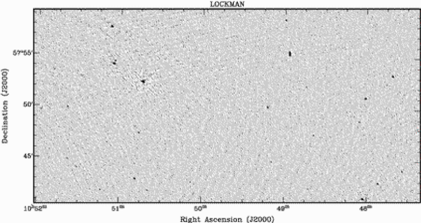
Figure 4: A 0.2 deg² region of the 610-MHz mosaic, illustrating the image quality. The grey-scale ranges between $-0.2$ and 1.0 mJy beam^-1, and the noise is relatively uniform and around 70 $\mu$Jy beam^-1, apart from small regions near bright sources where the noise increases. The brightest source in the field is GMRTLH J105043.2$+$575231, with a peak brightness of 50.4 mJy beam^-1.

3.1 Catalogue creation

An initial catalogue of 5223 sources was created using SExtractor. The mosaic was cut off at the point where the primary beam correction dropped to 20 per cent of its central value, but only sources inside the 30 per cent region were included in the catalogue to avoid the mosaic edges from affecting the local noise estimation. The requirements for a source to be included in the initial catalogue were that it had at least 5 connected pixels with brightness greater than 3 times the local noise $\sigma$, and a peak brightness greater than 6$\sigma$. The image pixel size meant that the beam was reasonably oversampled, so the source peak was taken to be the value of the brightest pixel within a source. The integrated flux density was calculated using the FLUX_AUTO option within SExtractor, which creates an elliptical aperture around each object (as described in Kron, 1980), and integrates the flux contained within the ellipse.

Artefacts are seen near bright sources which may be included in the initial catalogue. We used the technique described in Garn et al. (2008) in order to identify regions that are affected by these artefacts, and within these areas required sources to have a peak brightness greater than 12$\sigma$ in order to be included in the final catalogue. All sources with peaks greater than 10 mJy beam^-1 were examined for artefacts. The final catalogue contains 2845 sources – we have erred on the side of caution in order to produce a catalogue with little contamination from spurious sources.

Table 1 presents a sample of 10 entries in the catalogue, which is sorted by RA. The full table is available as Supplementary Material to the online version of this article, and via http://www.mrao.cam.ac.uk/surveys/. Column 1 gives the IAU designation of the source, in the form GMRTLH Jhhmmss.s$+$ddmmss, where J represents J2000.0 coordinates, hhmmss.s represents RA in hours, minutes and truncated tenths of seconds, and ddmmss represents the Dec. in degrees, arcminutes and truncated arcseconds. Columns 2 and 3 give the RA and Dec. of the source, calculated using first moments of the relevant pixel brightnesses to give a centroid position. Column 4 gives the brightness of the peak pixel in each source, in mJy beam^-1, and column 5 gives the local rms noise in $\mu$Jy beam^-1. Columns 6 and 7 give the integrated flux density and error, calculated from the local noise level and source size. Columns 8 and 9 give the $X$, $Y$ pixel coordinates from the mosaic image of the source centroid. Column 10 is the SExtractor deblended object flag – 1: where a nearby bright source may be affecting the calculated flux, 2: where a source has been deblended into two or more components from a single initial island of flux, and 3: when both of the above criteria apply. There are 77 sources present in our catalogue with non-zero deblend flags, and it is necessary to examine the images to distinguish between the case where one extended object has been represented by two or more entries, and where two astronomically distinct objects are present.

Table 1: A sample of 10 entries from the 610-MHz Lockman Hole catalogue, sorted by ascending RA. The full version of this table is available as Supplementary Material to the online version of this article, and via http://www.mrao.cam.ac.uk/surveys/.

Name	RA	Dec.	Peak	Local Noise	Int. Flux Density	Error	$X$	$Y$	Flags
	J2000.0	J2000.0	mJy beam-1	$\mu$Jy beam-1	mJy	mJy
(1)	(2)	(3)	(4)	(5)	(6)	(7)	(8)	(9)	(10)
GMRTLH J104237.0$+$583759	10:42:37.04	$+$58:37:59.1	0.564	82	1.666	0.136	3994	4773	0
GMRTLH J104237.1$+$572634	10:42:37.10	$+$57:26:34.7	0.539	88	0.473	0.072	4018	1917	0
GMRTLH J104237.4$+$574652	10:42:37.41	$+$57:46:52.1	0.445	68	0.412	0.056	4010	2729	3
GMRTLH J104238.3$+$572630	10:42:38.36	$+$57:26:30.7	0.698	88	0.586	0.082	4012	1914	0
GMRTLH J104239.2$+$585011	10:42:39.27	$+$58:50:11.5	0.536	73	0.626	0.085	3978	5261	0
GMRTLH J104239.3$+$572752	10:42:39.35	$+$57:27:52.1	0.545	78	0.643	0.081	4006	1969	0
GMRTLH J104240.6$+$580353	10:42:40.62	$+$58:03:53.6	0.438	71	0.786	0.083	3987	3409	0
GMRTLH J104240.6$+$573836	10:42:40.65	$+$57:38:36.5	0.410	60	0.331	0.054	3995	2398	0
GMRTLH J104241.4$+$580505	10:42:41.46	$+$58:05:05.9	0.648	77	0.710	0.082	3982	3458	0
GMRTLH J104241.6$+$573259	10:42:41.63	$+$57:32:59.6	0.547	78	0.518	0.078	3992	2173	0

3.2 Comparison with the FIRST survey

In order to test the positional accuracy of our catalogue, we paired it with sources in the FIRST survey (Becker et al., 1995). The whole of our 610-MHz survey region is covered by FIRST, and 340 sources are found with positions within 6 arcsec in the two surveys. The difference in source positions in the GMRT catalogue relative to the VLA FIRST survey is approximately Gaussian, with mean offset of 0.01 arcsec in RA and $-0.1$ arcsec in Dec. The standard deviations of the distribution are 0.3 and 0.5 arcsec respectively. We make no alteration to the coordinates of sources in our survey due to the good agreement in positions.

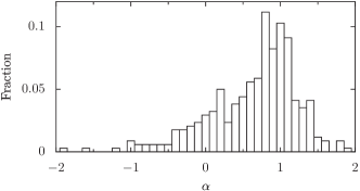
Figure 5: Radio spectral index $\alpha$ between 610 MHz and 1.4 GHz, for sources in the FIRST catalogue.

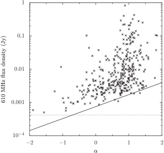
Figure 6: The variation in spectral index $\alpha$ with 610-MHz flux density. Crosses represent sources in the GMRT and FIRST catalogues, with the solid black line showing the limiting spectral index that could be detected, given the respective sensitivity levels. The 610-MHz flux density limit is shown by the dotted black line.

The spectral index distribution of the matched sources is shown in Fig. 5, using the integrated flux density measurements. The distribution peaks around $\alpha=0.8$, where $\alpha$ is defined so that the flux density $S$ scales with frequency $\nu$ as $S=S_{0}\nu^{-\alpha}$. There are significant biases in this distribution due to the differing sensitivity levels of the two surveys – Fig. 6 shows the variation in spectral index with the 610-MHz flux density. Below a few mJy, steep spectrum sources that are visible at 610 MHz cannot be detected in the FIRST survey, due to its limited depth (shown by the solid line).

3.3 Sub-millimetre galaxies

Biggs & Ivison (2007) have produced a sample of 12 sub-millimetre galaxies (SMGs) detected with combined VLA and Multi-Element Radio-Linked Interferometer (MERLIN) observations at 1.4 GHz. The majority of sources have a flux density at 1.4 GHz less than 150 $\mu$Jy, but there are three ‘bright’ sources, SMG06, SMG10 and SMG11 with 1.4-GHz flux densities of 246, 295 and 249 $\mu$Jy respectively, and typical errors of $\sim 10$ $\mu$Jy. One of these (SMG10, at $z=1.212$) is detected in the 610-MHz catalogue with a flux density of $538\pm 83$ $\mu$Jy, giving it a spectral index of $\alpha=0.72\pm 0.19$. The remaining two radio-bright SMGs, and all of the faint ones, are undetected at 610 MHz. The 610-MHz noise level at the location of the two undetected bright SMGs is approximately 100 $\mu$Jy beam^-1, leading to an upper limit on the spectral index of these sources of $\alpha=1.05$.

4 Differential source counts

We calculated source counts for the Lockman Hole using a method similar to the one used for the ELAIS-N1 field (Garn et al., 2008), by deriving faint and bright source counts from two separate regions of the mosaic. In order to calculate source counts below 10 mJy, we chose a $75\times 75$ arcmin² region that was relatively free from bright sources above 10 mJy (and consequently from the errors resulting from those sources). For reliability, source counts were constructed from all sources with a signal-to-noise ratio greater than 7, and binned by their integrated flux density, using the same flux density bins as in Garn et al. (2008). The lowest flux bin went down to 556 $\mu$Jy, corresponding to the approximate noise of 80 $\mu$Jy beam^-1 within the selected region. We calculated the differential source count for sources with flux densities above 10 mJy by considering the central $\sim$3.3 deg² of the map, excluding the region near pointing 10 which had significantly greater noise. Within this area, residual sidelobes are seen from several bright sources, but inspection of the residuals found them to have a typical flux density of below 1 mJy, which will not affect the source counts.

The differential source counts ${\rm d}N/{\rm d}S$ were corrected for the fraction of the image over which they could be detected, taking into account the increase in noise near the bright sources. In order to correct for resolution bias, we applied a correction factor of 3 per cent for source counts below 1 mJy (Moss et al., 2007). No correction for resolution bias was made for brighter sources. Table 2 gives the source counts, mean flux density $\langle S\rangle$ of sources in each bin, ${\rm d}N/{\rm d}S$ and ${\rm d}N/{\rm d}S$ normalised by $\langle S\rangle^{2.5}$, the value expected from a static Euclidean universe, along with Poisson error estimates calculated from the number of sources detected in each flux density bin. The source counts are consistent with our results from the Spitzer extragalactic First Look Survey and ELAIS-N1 fields (Garn et al., 2007; Garn et al., 2008), and in Table 3 we give the source counts found by combining data from the three fields.

Table 2: 610-MHz differential source counts for the Lockman Hole survey.

Flux Bin	$\langle S\rangle$	$N$	$N_{\rm c}$	${\rm d}N/{\rm d}S$	${\rm d}N/{\rm d}S~{}\langle S\rangle^{2.5}$
(mJy)	(mJy)			(sr-1 Jy-1)	(sr-1 Jy1.5)
0.556 – 0.798	0.674	94	108.8	$9.4\pm 1.0\times 10^{8}$	$11.1\pm 1.2$
0.798 – 1.145	0.951	61	61.3	$3.7\pm 0.5\times 10^{8}$	$10.4\pm 1.3$
1.145 – 1.643	1.381	31	31.0	$1.3\pm 0.2\times 10^{8}$	$9.3\pm 1.7$
1.643 – 2.358	1.992	27	27.0	$7.9\pm 1.5\times 10^{7}$	$14.0\pm 2.7$
2.358 – 3.384	2.909	26	26.0	$5.3\pm 1.0\times 10^{7}$	$24.3\pm 4.8$
3.384 – 4.856	3.981	14	14.0	$2.0\pm 0.5\times 10^{7}$	$20.0\pm 5.3$
4.856 – 6.968	5.700	9	9.0	$8.9\pm 3.0\times 10^{6}$	$21.9\pm 7.3$
6.968 – 10.00	8.429	6	6.0	$4.2\pm 1.7\times 10^{6}$	$27.1\pm 11.1$
10.00 – 13.49	11.70	14	14.0	$4.0\pm 1.1\times 10^{6}$	$59.3\pm 15.9$
13.49 – 18.20	15.70	8	8.0	$1.7\pm 0.6\times 10^{6}$	$52.5\pm 18.6$
18.20 – 24.56	20.71	17	17.0	$2.7\pm 0.7\times 10^{6}$	$165\pm 40.0$
24.56 – 33.14	27.65	11	11.0	$1.3\pm 0.4\times 10^{6}$	$163\pm 49.2$
33.14 – 44.72	37.70	7	7.0	$6.0\pm 2.3\times 10^{5}$	$167\pm 63.1$
44.72 – 60.34	57.47	2	2.0	$1.3\pm 0.9\times 10^{5}$	$101\pm 71.7$
60.34 – 81.41	74.23	4	4.0	$1.9\pm 1.0\times 10^{5}$	$285\pm 142$
81.41 – 109.8	94.89	4	4.0	$1.4\pm 0.7\times 10^{5}$	$390\pm 195$
109.8 – 148.2	120.5	3	3.0	$7.8\pm 4.5\times 10^{4}$	$395\pm 228$
148.2 – 200.0	160.3	1	1.0	$1.9\pm 1.9\times 10^{4}$	$199\pm 199$

Table 3: Average 610-MHz differential source counts for the Spitzer extragalactic First Look, ELAIS-N1 and Lockman Hole surveys.

Flux Bin	$\langle S\rangle$	$N$	$N_{\rm c}$	${\rm d}N/{\rm d}S$	${\rm d}N/{\rm d}S~{}\langle S\rangle^{2.5}$
(mJy)	(mJy)			(sr-1 Jy-1)	(sr-1 Jy1.5)
0.270 – 0.387	0.331	269	399.6	$3.8\pm 0.2\times 10^{9}$	$7.6\pm 0.5$
0.387 – 0.556	0.463	269	287.2	$1.9\pm 0.1\times 10^{9}$	$8.8\pm 0.5$
0.556 – 0.798	0.669	268	288.3	$8.7\pm 0.5\times 10^{8}$	$10.1\pm 0.6$
0.798 – 1.145	0.958	172	172.3	$3.6\pm 0.3\times 10^{8}$	$10.3\pm 0.8$
1.145 – 1.643	1.365	125	125.0	$1.8\pm 0.2\times 10^{8}$	$12.6\pm 1.1$
1.643 – 2.358	1.951	84	84.0	$8.6\pm 0.9\times 10^{7}$	$14.5\pm 1.6$
2.358 – 3.384	2.793	73	73.0	$5.2\pm 0.6\times 10^{7}$	$21.5\pm 2.5$
3.384 – 4.856	4.060	53	53.0	$2.6\pm 0.4\times 10^{7}$	$27.7\pm 3.8$
4.856 – 6.968	5.712	33	33.0	$1.1\pm 0.2\times 10^{7}$	$28.2\pm 4.9$
6.968 – 10.00	8.414	28	28.0	$6.8\pm 1.3\times 10^{6}$	$43.9\pm 8.3$
10.00 – 13.49	11.55	56	56.0	$5.5\pm 0.7\times 10^{6}$	$78.6\pm 10.5$
13.49 – 18.20	15.77	38	38.0	$2.8\pm 0.5\times 10^{6}$	$86.1\pm 14.0$
18.20 – 24.56	21.01	49	49.0	$2.6\pm 0.4\times 10^{6}$	$168\pm 24.1$
24.56 – 33.14	28.57	36	36.0	$1.4\pm 0.2\times 10^{6}$	$198\pm 33.0$
33.14 – 44.72	38.16	24	24.0	$7.1\pm 1.4\times 10^{5}$	$202\pm 41.2$
44.72 – 60.34	54.58	9	9.0	$2.0\pm 0.7\times 10^{5}$	$137\pm 45.7$
60.34 – 81.41	68.26	11	11.0	$1.8\pm 0.5\times 10^{5}$	$217\pm 65.5$
81.41 – 109.8	94.89	4	4.0	$4.8\pm 2.4\times 10^{4}$	$133\pm 66.7$
109.8 – 148.2	121.6	6	6.0	$5.3\pm 2.2\times 10^{4}$	$276\pm 113$
148.2 – 200.0	175.1	4	4.0	$2.6\pm 1.3\times 10^{4}$	$339\pm 170$

Fig. 7 shows the normalised differential source counts from our three survey fields, along with 610-MHz source counts from two other GMRT surveys (Moss et al., 2007; Bondi et al., 2007), and a collection of shallow surveys made with the Westerbork Synthesis Radio Telescope (WSRT; Valentijn et al., 1977; Katgert, 1979; Valentijn, 1980; Katgert-Merkelijn et al., 1985). The turnover in source counts is clearly visible below $\sim$2 mJy, due to the emergence of a new population of radio sources (see e.g. Simpson et al., 2006).

4.1 Source count models

Radio source counts have been used to understand the evolution of radio sources for many years (e.g. Longair, 1966). We model the source counts as being due to three distinct populations of radio sources, following Seymour, McHardy & Gunn (2004). The normalised differential source counts for a population with radio luminosity function (RLF) given by $\phi_{z}(L)$ can be calculated using

$$S^{2.5}\frac{{\rm d}N}{{\rm d}S}\propto S^{1.5}\int_{0}^{\infty}\phi_{0}(S,z)h(z)(1+z)^{P}{\rm d}z$$ (1)

where $\phi_{z}(L)$ has been separated into luminosity evolution $\phi_{0}(S,z)$ and density evolution $(1+z)^{P}$ terms, and the change in comoving volume with redshift is given by $h(z)$ – for more details, see Section 4.3 of Seymour et al. (2004).

The three populations of radio sources consist of a ‘steep’ spectrum AGN population with assumed spectral index of $\alpha=0.8$, a ‘flat’ spectrum AGN population with spectral index of 0 and a ‘starburst’ population, also assumed to have spectral index of 0.8. Following Seymour et al. (2004) we consider no density evolution $(P=0)$, and use the 1.4-GHz AGN luminosity functions and luminosity evolution from Rowan-Robinson et al. (1993), which is based on earlier work at 2.7 GHz by Dunlop & Peacock (1990). The AGN contribution to the radio source counts is therefore fixed at the same values found by previous authors, and dominates the source counts above a few mJy.

We obtain a local RLF for starburst galaxies from Mauch & Sadler (2007), measured from 4006 local radio sources present in the 6dF Galaxy Survey (Jones et al., 2005) and NVSS surveys, classified as starburst galaxies through their optical spectra. Following Hopkins et al. (1998) the starburst luminosity evolution is parameterised as $(1+z)^{Q}$, where we assume evolution takes place between $z=0$ and 2, based on measurements of the change in cosmic star formation rate across this redshift range (Madau et al., 1996; Hopkins & Beacom, 2006). The star formation rate is assumed to remain constant for $z>2$. An M82-type galaxy at $z=2$ would have a flux density below 1 $\mu$Jy at 1.4 GHz, and would therefore not contribute to the observed source counts, making this assumption valid.

We construct models for the source counts at 610 MHz and 1.4 GHz, with the 1.4-GHz RLFs converted to 610 MHz through the use of the spectral indices chosen above. Fig. 7 shows the predicted 610-MHz source counts from three models of pure luminosity evolution, with the starburst evolution parameter $Q$ taking the values 2, 2.5 and 3, in order to compare to previous works. The source count measurements at 1.4 GHz are taken from a wide range of surveys (White et al., 1997; Ciliegi et al., 1999; Gruppioni et al., 1999; Prandoni et al., 2001; Bondi et al., 2003; Hopkins et al., 2003; Seymour et al., 2004; Huynh et al., 2005; Biggs & Ivison, 2006; Simpson et al., 2006), and are shown in Fig. 8 along with the same three luminosity evolution models.

We find that a value of $Q$ between 2.5 and 3 agrees well with the data. From 1.4-GHz source counts, Rowan-Robinson et al. (1993) found $Q=3.1$, Condon, Cotton & Broderick (2002) found $Q=3\pm 1$, Seymour et al. (2004) found $Q=2.5\pm 0.5$ and Huynh et al. (2005) found $Q=2.7$. Using 1.4-GHz information and a range of other star formation indicators, Hopkins (2004) find $Q=2.7\pm 0.6$ and $P=0.15\pm 0.6$. Moss et al. (2007) use their 610-MHz source counts to fit a value of $Q=2.45^{+0.25}_{-0.4}$. Our results are therefore consistent with previous findings, and demonstrate that both sets of source counts can be modelled simultaneously with the same radio luminosity functions and evolutionary dependence.

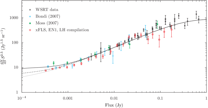
Figure 7: Differential source counts at 610 MHz (Valentijn et al., 1977; Katgert, 1979; Valentijn, 1980; Katgert-Merkelijn et al., 1985; Bondi et al., 2007; Moss et al., 2007; Garn et al., 2007; Garn et al., 2008), normalised by the value expected in a static Euclidean universe. Model source counts calculated with pure luminosity evolution with $Q$ = 2 (dotted line), 2.5 (dashed line) and 3 (solid line) are shown – see Section 4.1 for more details.

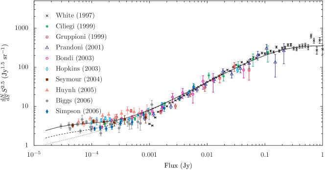
Figure 8: Differential source counts at 1.4 GHz (White et al., 1997; Ciliegi et al., 1999; Gruppioni et al., 1999; Prandoni et al., 2001; Bondi et al., 2003; Hopkins et al., 2003; Seymour et al., 2004; Huynh et al., 2005; Biggs & Ivison, 2006; Simpson et al., 2006), normalised by the value expected in a static Euclidean universe. Model source counts calculated with pure luminosity evolution with $Q$ = 2 (dotted line), 2.5 (dashed line) and 3 (solid line) are shown – see Section 4.1 for more details.

5 Conclusions

We have observed $\sim$5 deg² of the Lockman Hole with the GMRT at 610 MHz. The majority of the observations have a rms noise of $\sim$60 $\mu$Jy beam^-1 before primary beam correction, with the noise level increasing in the direction of a bright FIRST source outside of our image. A catalogue of 2845 radio source components detected above 6$\sigma$ has been presented, and the full catalogue and mosaic made available via http://www.mrao.cam.ac.uk/surveys/.

We calculate differential source counts at 610 MHz by considering two separate regions of the mosaic. The source counts are calculated between 556 $\mu$Jy and 200 mJy, and are shown to agree with previous 610-MHz source counts in other regions. We present average source counts calculated from this work and two previous surveys of the Spitzer extragalactic First Look Survey field and ELAIS-N1 field. The turnover in differential source counts is clearly visible below 2 mJy, and we show that a three-component population containing steep spectrum AGN, flat spectrum AGN and starburst galaxies which undergo pure luminosity evolution is sufficient to model the 610-MHz and 1.4-GHz source counts simultaneously.

References

- Adelman-McCarty et al. (2007) Adelman-McCarty J. K., et al., 2007, preprint (astro-ph/0707.3413)
- Ananthakrishnan (2005) Ananthakrishnan S., 2005, in Sripathi Acharya B., Gupta S., Jagadeesan P., Jain A., Karthikeyan S., Morris S., Tonwar S., eds, Proc. 29th Int. Cosmic Ray Conf. Vol. 10, Tata Institute of Fundamental Research, Mumbai. pp 125–136
- Appleton et al. (2004) Appleton P. N., et al., 2004, ApJS, 154, 147
- Baars et al. (1977) Baars J., Genzel R., Pauliny-Toth I., Witzel A., 1977, A&A, 61, 99
- Becker et al. (1995) Becker R. H., White R. L., Helfand D. J., 1995, ApJ, 450, 559
- Beichman et al. (2003) Beichman C. A., Cutri R., Jarrett T., Steining R., Skrutskie M., 2003, AJ, 125, 2521
- Bertin & Arnouts (1996) Bertin E., Arnouts S., 1996, A&AS, 117, 393
- Biggs & Ivison (2006) Biggs A. D., Ivison R. J., 2006, MNRAS, 371, 963
- Biggs & Ivison (2007) Biggs A. D., Ivison R. J., 2007, MNRAS, in press (astro-ph/0712.3047)
- Bondi et al. (2003) Bondi M., et al., 2003, A&A, 403, 857
- Bondi et al. (2007) Bondi M., et al., 2007, A&A, 463, 519
- Brunner et al. (2008) Brunner H., Cappelluti N., Hasinger G., Barcons X., Fabian A. C., Mainieri V., Szokoly G., 2008, A&A, 479, 283
- Bundy et al. (2007) Bundy K., et al., 2007, preprint, astro-ph/0710.2105
- Ciliegi et al. (1999) Ciliegi P., et al., 1999, MNRAS, 302, 222
- Ciliegi et al. (2003) Ciliegi P., Zamorani G., Hasinger G., Lehmann I., Szokoly G., Wilson G., 2003, A&A, 398, 901
- Condon (1992) Condon J. J., 1992, ARA&A, 30, 575
- Condon et al. (2002) Condon J. J., Cotton W. D., Broderick J. J., 2002, AJ, 124, 675
- Condon et al. (1998) Condon J. J., Cotton W. D., Yin Q. F., Perley R. A., Taylor G. B., Broderick G. B., 1998, AJ, 115, 1693
- Coppin et al. (2006) Coppin K., et al., 2006, MNRAS, 372, 1621
- de Ruiter et al. (1997) de Ruiter H. R., et al., 1997, A&A, 319, 7
- Dunlop & Peacock (1990) Dunlop J. S., Peacock J. A., 1990, MNRAS, 247, 19
- Fazio et al. (2004) Fazio G., et al., 2004, ApJS, 154, 10
- Garn et al. (2008) Garn T., Ford D. C., Alexander P., 2008, MNRAS, submitted
- Garn et al. (2007) Garn T., Green D. A., Hales S. E. G., Riley J. M., Alexander P., 2007, MNRAS, 376, 1251
- Garn et al. (2008) Garn T., Green D. A., Riley J. M., Alexander P., 2008, MNRAS, 383, 75
- Garrett (2002) Garrett M. A., 2002, A&A, 384, L19
- Gruppioni et al. (1999) Gruppioni C., et al., 1999, MNRAS, 305, 297
- Hasinger et al. (1998) Hasinger G., Burg R., Giacconi R., Schmidt M., Trümper J., Zamorani G., 1998, A&A, 329, 482
- Hasinger et al. (2001) Hasinger G., et al., 2001, A&A, 365, L45
- Helou et al. (1985) Helou G., Soifer B. T., Rowan-Robinson M., 1985, ApJ, 298, L7
- Holland et al. (1999) Holland W. S., et al., 1999, MNRAS, 303, 659
- Hopkins (2004) Hopkins A. M., 2004, ApJ, 615, 209
- Hopkins et al. (2003) Hopkins A. M., Alfonso J., Chan B., Cram L. E., Georgakakis A., Mobasher B., 2003, AJ, 125, 465
- Hopkins & Beacom (2006) Hopkins A. M., Beacom J. F., 2006, ApJ, 651, 142
- Hopkins et al. (1998) Hopkins A. M., Mobasher B., Cram L., Rowan-Robinson M., 1998, MNRAS, 296, 839
- Huynh et al. (2005) Huynh M. T., Jackson C. A., Norris R. P., Prandoni I., 2005, AJ, 130, 1373
- Ibar et al. (2008) Ibar E., et al., 2008, MNRAS, in press (astro-ph/0802.2694v2)
- Jones et al. (2005) Jones D. H., Saunders W., Read M., Colless M., 2005, PASA, 22, 277
- Kantharia & Rao (2001) Kantharia N., Rao A., 2001, GMRT Technical Note R00185
- Katgert (1979) Katgert J. K., 1979, A&A, 73, 107
- Katgert-Merkelijn et al. (1985) Katgert-Merkelijn J. K., Windhorst R. A., Katgert P., Robertson J. G., 1985, A&AS, 61, 517
- Kron (1980) Kron R. G., 1980, ApJS, 43, 305
- Lawrence et al. (2007) Lawrence A., et al., 2007, MNRAS, 379, 1599
- Lockman et al. (1986) Lockman F. J., Jahoda K., McCammon D., 1986, ApJ, 302, 432
- Longair (1966) Longair M. S., 1966, MNRAS, 133, 421
- Lonsdale et al. (2003) Lonsdale C., et al., 2003, PASP, 115, 897
- Madau et al. (1996) Madau P., Ferguson H. C., Dickinson M. E., Giavalisco M., Steidel C. C., Fruchter A., 1996, MNRAS, 283, 1388
- Mainieri et al. (2002) Mainieri V., Bergeron J., Hasinger G., Lehmann H., Rosati P., Schmidt M., Szokoly G., Della Ceca R., 2002, A&A, 393, 425
- Mauch & Sadler (2007) Mauch T., Sadler E. M., 2007, MNRAS, 375, 931
- Moss et al. (2007) Moss D., Seymour N., McHardy I. M., Dwelly T., Page M. J., Loaring N. S., 2007, MNRAS, 378, 995
- Murphy et al. (2006) Murphy E. J., et al., 2006, ApJ, 638, 157
- Polletta et al. (2006) Polletta M., et al., 2006, The X-ray Universe 2005, 604, 807
- Prandoni et al. (2001) Prandoni I., Gregorini L., Parma P., de Ruiter H. R., Vettolani G., Wieringa M. H., Ekers R. D., 2001, A&A, 365, 392
- Reike et al. (2004) Reike G., et al., 2004, ApJS, 154, 25
- Richards et al. (2007) Richards A., et al., 2007, A&A, 472, 805
- Rowan-Robinson et al. (1993) Rowan-Robinson M., Benn C. R., Lawrence A., McMahon R. G., Broadhurst T. J., 1993, MNRAS, 263, 123
- Rowan-Robinson et al. (2008) Rowan-Robinson M., et al., 2008, MNRAS, in press (astro-ph/0802.1890v1)
- Seymour et al. (2004) Seymour N., McHardy I. M., Gunn K. F., 2004, MNRAS, 352, 131
- Simpson et al. (2006) Simpson C., et al., 2006, MNRAS, 372, 741
- Surace et al. (2005) Surace J. A., et al., 2005, The SWIRE Data Release 2: Image Atlases and Source Catalogues for ELAIS-N1, ELAIS-N2, XMM-LSS and the Lockman Hole, SWIRE DR2 online data paper
- Tasse et al. (2007) Tasse C., Röttgering H. J. A., Best P. N., Cohen A. S., Pierre M., Wilman R., 2007, A&A, 471, 1105
- Valentijn (1980) Valentijn A. E., 1980, A&A, 89, 234
- Valentijn et al. (1977) Valentijn E. A., Jaffe W. J., Perola G. C., 1977, A&A, 28, 333
- Vlahakis et al. (2007) Vlahakis C., Eales S., Dunne L., 2007, MNRAS, 379, 1042
- Werner et al. (2004) Werner M., et al., 2004, ApJS, 154, 1
- White et al. (1997) White R. L., Becker R. H., Helfand D. J., Gregg M. D., 1997, ApJ, 475, 479