Energy spectra for protons

emitted in the reaction

${}^{\textrm{nat}}{\textrm{Ca}}(\textrm{n},x\textrm{p})$ at 94 MeV

Pär-Anders Söderström

Abstract

The MEDLEY setup based at The Svedberg Laboratory (TSL), Uppsala, Sweden has previously been used to measure double-differential cross sections for elastic $nd$ scattering, as well as light ion production reactions for various nuclei in the interaction with neutrons around 95 MeV. When moved to the new beam line, the first experimental campaign was on light-ion production from Ca at 94 MeV in February 2005.

These data sets have been analyzed for proton production in forward and backward angles. The $\Delta E-\Delta E-E$ technique have been used to identify protons, and a cutoff as low as 2.5 MeV is achieved. Suppression of events induced by neutrons in the low-energy tail of the neutron field is achieved by time-of-flight techniques. The data are normalized relative to elastic $np$ scattering measured in the 20-degree telescope. Results from an accepted neutron spectrum are presented and some methods to correct for events from low energy neutrons are presented and evaluated. The data are compared with calculations using the nuclear code TALYS. It was found that TALYS systematically overestimates the compound part, and underestimates the pre-equilibrium part of the cross section.

List of acronyms

ADC

analog-to-digital converter

BD

beam dump

CFD

constant fraction discriminator

CM

center of mass

CsI(Tl)

thallium activated cesium iodide

DWBA

distorted wave Born approximation

FIFO

fan-in/fan-out

FWHM

full width at half maximum

ICM

ionization chamber monitor

INF

Department of Neutron Physics, Uppsala University

LET

linear-energy-transfer

NN

Nucleon-Nucleon

OMP

optical model potential

PWA

partial wave analysis

QDC

charge-to-digital converter

RF

radio-frequency

SRIM

The Stopping and Range of Ions in Matter

T1

Telescope 1

T2

Telescope 2

T7

Telescope 7

T8

Telescope 8

TDC

time-to-digital converter

TFBC

thin-film breakdown counter

TOF

time-of-flight

TSL

The Svedberg Laboratory

List of Figures

1. 1.1 $\beta$-decay of a free neutron
2. 1.2 Man as a source for radiation
3. 1.3 Reparation errors and DNA-damage
4. 2.1 The different types of reactions
5. 2.2 Optical potentials plotted for ⁴⁰Ca and incoming neutrons.
6. 2.3 Different reaction paths in the two component exciton model
7. 3.1 Drawing of the new neutron beam facility in the Blue Hall
8. 3.2 The exit of the collimator
9. 3.3 The MEDLEY spectrometer
10. 3.4 One of the aluminum frames and the CH₂ target
11. 3.5 One of the detector telescopes
12. 3.6 Stopping and range of protons in silicon
13. 3.7 MEDLEY electronics
14. 4.1 Calibrated $\Delta E_{1}$-$\Delta E_{2}$ and $\Delta E_{2}$-$E$ plots for T1
15. 4.2 RF 1 versus RF 2
16. 4.3 Scematic illustration of the two RF signals
17. 4.4 First graphical selection cuts for protons
18. 4.5 Refined selection cuts for protons
19. 4.6 Neutron TOF versus proton energy
20. 4.6 Corrections
21. 4.9 Signal and background plots
22. 4.10 Target correction results
23. 4.11 Accepted neutron spectrum
24. 4.12 Elastic np peak
25. 5.1 Experimental double-differential cross sections
26. 5.2 Experimental angular-differential cross sections
27. 5.3 Experimental energy-differential cross sections
28. 6.1 TOF shift in T1 and run 37 in T8
29. 6.2 Mismatch between T1 and T8
30. 6.6 Different approaches to angular distributions
31. 6.6 Double- and energy-differential cross sections with experimental data subtracted
32. 6.7 Double- and energy-differential cross sections with TALYS data subtracted
33. 6.8 Double- and energy-differential cross sections with modified TALYS data subtracted
34. A.1 Contributions to total cross section from various reaction types
35. A.2 Typical sequence of hexadecimal raw data for an event
36. B.3 Scattering in the laboratory frame

List of Tables

1. 2.1 OMP parameters for ⁴⁰Ca
2. 4.1 Thickness and punch through energies for the different silicon detectors used.
3. 4.2 Stopping of protons in calcium
4. 4.3 Accepted neutron spectrum
5. 6.1 Angular-differential and total cross sections with subtracted data
6. 6.2 Systematic uncertainties
7. A.1 Detector setup
8. A.2 Runs with table at 180 degrees
9. A.3 Runs with table at 0 degrees
10. A.4 Calibration values
11. A.5 Energy binning for carbon subtraction
12. A.6 Experimental double-differential cross sections at 20 degrees
13. A.7 Experimental double-differential cross sections at 40 degrees
14. A.8 Experimental double-differential cross sections at 140 degrees
15. A.9 Experimental double-differential cross sections at 160 degrees
16. A.10 Experimental energy-differential cross sections
17. A.11 Experimental angular-differential cross sections
18. A.12 Experimental total cross sections

1 Introduction

In the last years, fast neutrons have gathered more and more interest worldwide. Lots of applications involving fast neutrons in some way are predicted to be available within 50 years, for example one can mention fusion power reactors and transmutation of spent nuclear fuel. Even today, fast neutrons play an important role in the field of electronics, where it can cause so called single event effects, doing damage to the hardware and software. Fast neutrons are also used for hadronic radiotherapy of cancer in several places in the world, for exampel at iTemba LABS in South Africa. So understanding of fast neutron interactions is a large and important part of applied nuclear physics.

In this work the interaction between 94 MeV neutrons with calcium will be examined, in particular the productions of protons at forward and backward angles. A first rough estimation of the angular distributions will also be carried out. In this introduction to the work, some general properties of the neutron, and experiments with the neutron, will be discussed, as well as a short introduction to the nucleus under study. This is followed by a few sections about what is actually measured and some possible applications and motivations for this work in the form of a biological introduction.

1.1 The neutron

The second lightest (known) baryon in the universe is the uncharged neutron, discovered in 1932 by James Chadwick [1], when he was examining mysterious radiation emitted from beryllium, boron and lithium that had been discovered a few years earlier by Bothe and Becker [2]. Since the neutron is the second lightest, the slight mass difference between it and the lightest, the proton, makes the neutron unstable when it is in an unbound state and it decays according to figure 1.1 with a lifetime of 887 seconds [3].

Figure 1.1: $\beta$-decay of a free neutron into a proton, an electron and an antineutrino.

The neutron interacts with its surroundings through all four of the fundamental forces: the strong nuclear force, the weak nuclear force, the electromagnetic force and the gravitational force. In experiments with neutrons there exist a few difficulties that do occur due to its special properties. Acceleration of neutrons is impossible today since accelerators use the charge of the particles. Instead, one has to rely on a neutron beam as a secondary beam. This means that one uses a primary beam of charged particles, for example protons, and let them hit some target that can induce a neutron production nuclear reaction. Similarly the focusing of particle beams is done by large magnets, while the beam shaping for a beam of uncharged particles must be done with collimators. Dealing with neutrons also gives rise to background and radiation protection issues. This since high-energy neutrons has a lower probability than charged particles for interaction and higher possibility for passing through the shielding material.

1.2 Calcium

The nucleus under study in this work builds up a quite hard, silvery white, alkaline earth metal. The name calcium origins from the Latin word calcis that means lime, referring to the group of minerals dominated by calcium-carbonates, -oxides and -hydroxides often used as building material, for example in limestone, concrete and mortar between bricks in masonry [5].

In the human body, calcium is the most common mineral where almost all of it is located in the skeleton in the form of hydroxide apatite crystals. The skeleton of a normal adult contains about 1 kg of calcium. Some of it can also be found in the soft tissue in the form of Ca²⁺ ions [6]. There are six stable isotopes of calcium where the doubly magic isotope ⁴⁰Ca is the absolutely most common one, with a natural abundance of 96.941 % [3].

1.3 Cross-section measurements

One of the most fundamental needs in nuclear physics, as well as in all other physics and even all other sciences, is theoretical models to explain nature. Of course, another fundamental need in the field of science is also the to go the other way, by obtaining experimental data to verify theoretical models.

In nuclear and particle physics the cross section is in a way the connection between everyday life and the often complicated and abstract theoretical models. It is a quantity that both can be measured in experiments, as well as calculated from simple or complex nuclear models. The unit is a non-SI, although accepted for use with the SI, areal unit named barn that can be visualized as the effective area a projectile sees when approaching a target. This makes the interpretation of a cross section as a reaction probability a little more intuitive; the larger the effective area of the target – the larger the probability of hitting it. It is important to keep in mind though that the reaction cross section is not the same as the geometric cross section.

1.4 Ionizing radiation and humans

The human body is constantly exposed to radioactivity in terms of ionizing radiation. The sources are partly due to human activities like rest products from atmospheric nuclear weapons tests, nuclear power accidents, dental x-rays and many other things. But there are also various natural sources of radioactivity. For example radon gas from earths crust and cosmic radiation. Even man itself contains various radioactive isotopes and is a source for radiation, as illustrated in figure 1.2.

Figure 1.2: In some sense, everyone of us is a Radioactive Man [8].

The damage that ionizing radiation does on human tissue is mainly on the DNA and a majority of the DNA damage is indirect by ionizing the water in the cell and creating very reactive free radicals. Following [9], there are three possible damages that can occur, namely base pair damage, single strand break and double strand break. Base pair damage and single strand break are the most common of these three, but causes generally no problems for the cell and are fixed fast and easy. Double strand break on the other hand can create some more severe problems.

When the DNA, in the form of chromosomes, gets exposed to a double strand break and the cell tries to repair it there are three possible outcomes. The first is that the reparation succeeds and everything is back to normal, but the reparation can also go wrong in two different ways. One way is that we get an abnormal chromosome, like a ring chromosome where the end of each arm has been lost and repaired into a ring formation. Another abnormal chromosome, that will appear in about 60 % of chromosome aberrations, is the di-centric chromosome where the chromosome has been repaired into one with two centromeres, the region where the two the two identical parts of the chromosome touch during cell division, instead of just one. Both these examples of abnormal chromosomes are, although fatal to the cell, quite harmless to humans since the damaged cell never can survive mitosis, cell division. This is illustrated in figure 1.3.

The third outcome, also illustrated in figure 1.3, of a double strand break is the worst one. Here the chromosomes undergo stable rearrangements instead of getting abnormal shapes. The stable rearrangements could consist of translocation of two of the arms or that a small portion of an arm is removed from the chromosome. This mutation does not lead to mitotic cell death. Instead the damage will multiply at the same rate as the cell, something that very well can be a part of inducing a cancer tumor. This is the reason why cancer-inducing effects are often refereed to as stochastic effects. The probability of the statistically rare event of mutation increases with increasing exposure, but the effect of an injury is independent of the received dose.

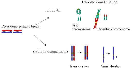
Figure 1.3: Possible reparation errors when fixing a double strand break and the resulting DNA-damage [10].

1.5 Cancer therapy

In principle there are three ways to treat cancer. One can use surgery, chemotherapy or radiation therapy. The basics behind radiation therapy of cancer are to damage the cancer cells DNA strands and in that way prevent the cell to divide. In this case one actually wants a double strand break that ends up in an abnormal chromosome and prevents the mitosis, as mentioned in section 1.4. The most common type of radiation therapy is using $\gamma$-rays from ⁶⁰Co, x-rays or electron beams. However some tumors, called radioresistant tumors, seem to respond quite poorly to this treatment and therefore other methods are needed.

One way is to use hadrons such as protons, neutrons, helium ions or pions instead of photons or electrons. Since hadrons have a larger linear-energy-transfer (LET), that is the stopping power in the medium, than electrons and photons, they has a higher chance to do biological damage to the cell. Actually there are three things that make a high LET particle more effective than a low LET particle. Firstly it is harder for the cells to repair the larger damage, secondly high LET particles is more efficient in damaging the oxygen-poor tissue in a tumor. And finally high LET radiation is not as sensitive to whether or not the cell is currently dividing as low LET radiation [9, 11]. Another property of charged hadrons is the interaction depth. While photons and neutrons deposit most of their energy in the surface, charged hadrons deposit most of their energy in a well-defined depth in the patient. This known as the Bragg peak.

Using fast neutrons for cancer therapy is a little more complex method than using photons, electrons or hadrons, since neutrons do not damage the tissue via direct interactions. Instead, nuclear reactions with neutrons damage the tissue indirectly by production of various types of light ions. This means that in order to make accurate dose calculations, typically via Monte Carlo based radiation transport codes, it is fundamental that the double-differential cross sections for light ion production are well known [12].

1.6 TALYS

TALYS is a joint project between NRG Petten in the Netherlands and CEA Bruyéres-le-Chétel in France, and is a nuclear reactions modelling program working with nuclear reactions of energies 1 keV - 200 MeV. It is written completely from scratch in Fortran77, with the only exception of the implemented coupled-channels code ECIS-97 [13].

The two main purposes of TALYS are to be used as a physics tool during experimental analysis, and as a data tool to generate nuclear data for use in various applications. The program is also very flexible, since one can get a reasonable cross section by a minimal input like the four lines:

projectile n
element    Ca
mass       40
energy     94

But it also reacts to more than 150 keywords, making it possible to adjust the nuclear models and the output [14].

2 Theory

As mentioned in section 1.6 the theoretical predictions are made using a nuclear reactions code called TALYS. This is an outline of how TALYS does the calculations in this particular case, after a brief introduction to the basics of nuclear reactions.

One should remember that this is only a crude simplification of the calculation process valid only for incident high-energy neutrons on a spherical nucleus and emission of protons. When dealing with more complex particles like deuterons, tritons, helium isotopes and so on effects like continuum stripping, pick-up and knock-out also needs to be taken into account. Deformed nuclei also introduce a number of corrections not needed here. An example of the different reactions contribution to the total cross section can be found in figure A.1.

2.1 The shell model and magic nuclei

In nuclear physics there is not a single simple model to describe the atomic nucleus completely. Instead several different models that fit different kinds of parameters or properties for the nuclei are used. For example there are the liquid drop model and the shell model.

The shell model for nuclei is quite analogous to the shell model for atoms. In the atomic shell model the electrons populate shells outside the nucleus and when a shell is filled they start filling the next. In a nucleus the principle is the same, only here it is protons and neutrons that occupy shells and not electrons. Since the neutron and the proton have individual shells two layers of shells are filled in parallel [15].

Since the shell model deals with particles populating different energy levels there are some regions of extra interest and these are the nuclei with filled, or close to filled, shells. The nuclei with certain number of nucleons, corresponding to filled shells in the shell model, are found to be more tightly bound than others. These numbers of nucleons are commonly referred to as magic numbers and are: 2, 8, 20, 28, 50, 82 and 126. Nuclei containing filled shells are consequently called magic nuclei and nuclei with both protons and neutrons in filled shells are called double magic nuclei. Examples of double magic nuclei are ¹⁶O, ⁴⁰Ca, ⁴⁸Ca and ²⁰⁸Pb.

There are theories that also higher numbers of neutrons and of protons are magic numbers which would give rise to stable exotic nuclei such as ${}^{298}_{114}$Uuq, ${}^{304}_{120}$Ubn and ${}^{310}_{126}$Ubh in an island of stability among the otherwise highly unstable elements at the end of the periodic table [16].

2.2 Fundamental nuclear reactions

One important field of research to understand nuclear physics is the study of nuclear reactions. The general nuclear reaction is when an incoming particle, $a$, hits a target, $X$, causing the emission of a particle, $b$, and a recoil nucleus, $Y$. This can be written on the same form as a chemical reaction

$$a+X\rightarrow Y+b$$ (2.1)

or in a more compact form $X(a,b)Y$ where the $Y$ often is dropped. An example of a reaction could be

$$\textrm{p}+{{}^{7}\textrm{Li}}\rightarrow{{}^{4}\textrm{He}}+\alpha$$ (2.2)

or correspondingly ${{}^{7}\textrm{Li}}(\textrm{p},\alpha)$. One can now divide (2.1) into two subgroups, elastic and inelastic nuclear reactions. An elastic reaction is when $a=b$ and $X=Y$ in (2.1) and no energy is lost due to excitation of any of the components, while in an inelastic process the target gets excited and/or $a\neq b$.

When studying high-energy reactions, another way to classify nuclear reactions is in terms of the time scales at which they occur, or equivalently in terms of the number of collisions within the nucleus. The fastest reactions, with the fewest collisions, are called direct reactions and occur on time scales of about $10^{-22}$ s. Here the incoming projectile primarily interacts with the surface of the target. At the opposite end there is the compound reaction at time scales of about $10^{-16}-10^{-18}$ s [15], and in between these types pre-equilibrium reactions may occur. The spectrum of the different reactions is illustrated in figure 2.1, where also the corresponding shape of the cross section is sketched.

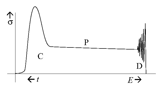
Figure 2.1: The different types of reactions, adapted from [14]: Compound reactions are indicated by C, pre-equilibrium reactions by P and direct reactions by D. The x-axis represent reaction time and particle energy and the y-axis the cross section.

2.3 The optical model

Before diving into details in the different nuclear reaction it is suitable to have a closer look at the basis of nuclear reaction calculations, something that is called the optical model potential (OMP). An analogy to this nuclear model is a murky glass sphere with some incoming light. Some of the light will be refracted, or elastically scattered, through the sphere, while other rays will be partially absorbed. In the nuclear model, this effect is mathematically described by defining a scattering potential as

$$\mathcal{U}(r,E)=\mathcal{V}(r,E)+i\mathcal{W}(r,E)$$ (2.3)

that can be inserted into the Schrödinger equation. Following the parametrisation in [14, 17], these potentials can in turn be described as a sum of potentials caused by different properties of the nucleus as

$$\mathcal{V}(r,E)=-\mathcal{V}_{V}(r,E)+\mathcal{V}_{SO}(r,E)\cdot\mathbf{L}\cdot\mathbf{\sigma}+\mathcal{V}_{C}(r)$$ (2.4a)

$$\mathcal{W}(r,E)=-\mathcal{W}_{V}(r,E)-\mathcal{W}_{D}(r,E)+\mathcal{W}_{SO}(r,E)\cdot\mathbf{L}\cdot\mathbf{\sigma}$$ (2.4b)

where the indices denote the volume part, $V$, the spin-orbit coupling part, $SO$, the surface derivative part, $D$, and the Coulomb part, $C$. Finally, all of these can be further broken down into an energy dependent part and a radial dependent form function part as follows

$$\mathcal{V}_{V}(r,E)=V_{V}(E)f(r,R_{V},a_{V})$$ (2.5a)

$$\mathcal{V}_{SO}(r,E)=V_{SO}(E)\left(\frac{\hbar}{m_{\pi}c}\right)^{2}\frac{1}{r}\frac{\textrm{d}}{\textrm{d}r}f(r,R_{SO},a_{SO})$$ (2.5b)

$$\mathcal{V}_{C}(r)=\left\{\begin{array}[]{cl}\frac{Zze^{2}}{2R_{C}}\left(3-\frac{r^{2}}{R_{C}^{2}}\right)&\text{for $r\leq R_{C}$}\\ \frac{Zze^{2}}{r}&\text{for $r\geq R_{C}$}\end{array}\right.$$ (2.5c)

$$\mathcal{W}_{V}(r,E)=W_{V}(E)f(r,R_{V},a_{V})$$ (2.5d)

$$\mathcal{W}_{D}(r,E)=-4a_{D}W_{D}(E)\frac{\textrm{d}}{\textrm{d}r}f(r,R_{D},a_{D})$$ (2.5e)

$$\mathcal{W}_{SO}(r,E)=W_{SO}(E)\left(\frac{\hbar}{m_{\pi}c}\right)^{2}\frac{1}{r}\frac{\textrm{d}}{\textrm{d}r}f(r,R_{SO},a_{SO}).$$ (2.5f)

The parameters $R_{i}=r_{i}A^{1/3}$ and $a_{i}$ are the radius and diffuseness parameters for the nucleus and the form function often is assumed to be of Woods-Saxon type

$$f(r,R_{i},a_{i})=\frac{1}{1+e^{\frac{r-R_{i}}{a_{i}}}}.$$ (2.6)

These parameters are listed by Koning and Delaroche [17] for a vast amount of nuclei and for ⁴⁰Ca and incoming neutrons they are given by table 2.1. The change in the potentials with energy of the incoming neutron and distance from the center of the nucleus is plotted in figure 2.2.

$r_{V}$	$a_{V}$	$r_{D}$	$a_{D}$	$r_{SO}$	$a_{SO}$
1.206	0.676	1.295	0.543	1.01	0.60
$V_{V}$	$V_{SO}$	$V_{C}$	$W_{V}$	$W_{D}$	$W_{SO}$
26.06	$3.984$	0	$8.216$	$1.597$	-0.9518

Table 2.1: Numerical values for the OMP parameters for ⁴⁰Ca with an incident neutron.

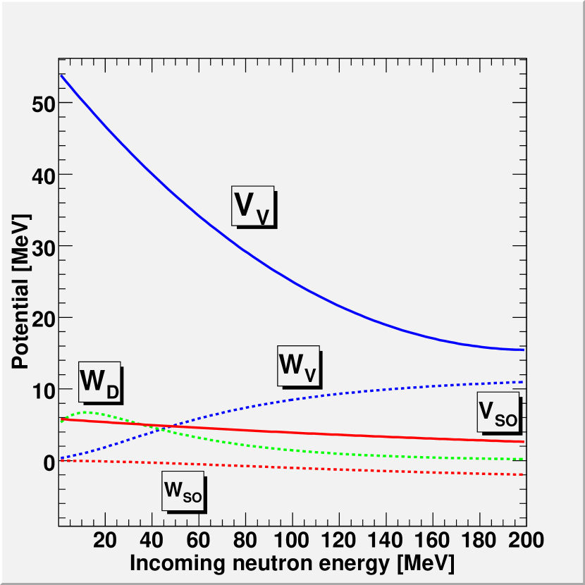
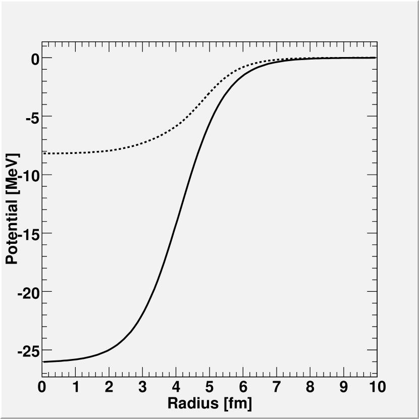
Figure 2.2: Optical potentials plotted for ⁴⁰Ca and incoming neutrons. The left panel shows $V_{V}(E)$, $V_{SO}(E)$, $W_{V}(E)$, $W_{D}(E)$ and $W_{SO}(E)$ for incident neutron energies between 0 and 200 MeV while the right panel shows $\mathcal{V}(r)$ (solid line) and $\mathcal{W}(r)$ (dashed line) for an energy of 94.5 MeV. Parametrized via [17].

2.4 Direct reactions

To calculate the cross sections from the direct formation processes TALYS has several models incorporated, like the weak coupling model or giant resonances. For near-spherical nuclides TALYS calculates the cross sections for the direct formation processes with the distorted wave Born approximation (DWBA). This basically means that one uses first order perturbation theory on the regular Born approximation, that the incoming and outgoing wave functions are just plane waves. This will give a result where the simple plane waves of the Born approximation is disturbed by the scattering potential of Eq. (2.3). This first order model for small deformations is valid since ⁴⁰Ca is a double magic nucleus, and hence near spherical. For a reaction like (2.1), the cross section is obtained from the relation

$$\frac{\textrm{d}\sigma^{\textrm{D}}}{\textrm{d}\Omega}=\frac{E_{a}E_{b}}{(2\pi)^{2}(\hbar c)^{4}}\frac{p_{b}}{p_{a}}\frac{1}{(2s_{a}+1)(2s_{X}+1)}\sum_{m_{a},m_{X},m_{b},m_{Y}}\left|\left\langle f\left|H_{\textrm{int}}\right|i\right\rangle\right|^{2}$$ (2.7)

where $E_{i}$ is the total energy, $p_{i}$ the momentum, $s_{i}$ the spin of the particle, $i$, and $m_{i}$ the mass. The initial and final states $\left\langle f\right|$ and $\left|i\right\rangle$ are given by the DWBA and $H_{\textrm{int}}$ is the interaction potential [18].

2.5 Pre-equilibrium reactions

After the direct reaction and before the nucleus reaches equilibrium some pre-equilibrium processes takes place. In TALYS the pre-equilibrium stage is calculated using a model called the two-component exciton model, following [14, 19]. In analogy to solid state physics one can define particle-hole pairs, also called pairs of excitons, above the Fermi surface as

$$n_{\pi}=p_{\pi}+h_{\pi}$$ (2.8a)

$$n_{\nu}=p_{\nu}+h_{\nu}$$ (2.8b)

$$p=p_{\pi}+p_{\nu}$$ (2.8c)

$$h=h_{\pi}+h_{\nu}$$ (2.8d)

$$n=n_{\pi}+n_{\nu}$$ (2.8e)

where $p$ is the number of particles, $h$ the number of holes and $n$ the number of excitons while $\pi$ corresponds to protons and $\nu$ to neutrons. When the incoming projectile interacts with the nucleus it can excite a particle-hole pair. On its path through the nucleus it can either excite new particle-hole pairs, annihilate existing ones or change configuration of the existing pairs as illustrated in figure 2.3, as well as release some excitation energy by emitting a particle.

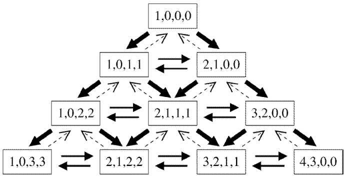
Figure 2.3: Different possible reaction paths in the two component exciton model for an incoming proton [19]. The numbers in the boxes correspond to $p_{\pi}$, $h_{\pi}$, $p_{\nu}$ and $h_{\nu}$ of some population $\mathcal{P}\left(p_{\pi},h_{\pi},p_{\nu},h_{\nu}\right)$. The thickness of the arrows is proportional to the transition rate, and as the arrows pointing backwards are really small compared to the others, they are neglected by TALYS. This is the so called never-come-back approximation.

The more interactions the particle undergoes on its way through the nucleus, the more it looses its memory of incoming direction and energy until it reaches some equilibrium state and the compound model takes over. The cross section for this pre-equilibrium state is described by

$$\frac{\textrm{d}\sigma_{k}^{\textrm{P}}}{\textrm{d}E_{k}}=\sigma^{\textrm{CF}}\sum_{p_{\pi}=p_{\pi}^{0}}^{p_{\pi}^{\textrm{max}}}\sum_{p_{\nu}=p_{\nu}^{0}}^{p_{\nu}^{\textrm{max}}}W_{k}\left(p_{\pi},h_{\pi},p_{\nu},h_{\nu},E_{k}\right)\tau\left(p_{\pi},h_{\pi},p_{\nu},h_{\nu}\right)P\left(p_{\pi},h_{\pi},p_{\nu},h_{\nu}\right)$$ (2.9)

where $\sigma^{\textrm{CF}}$ is the total compound formation cross section, $W_{k}$ is the emission rate, $\tau$ the lifetime of the particle-hole states and $P$ the states that survived and are left from the last process.

The total compound-formation cross section is just the reaction cross section, that can be calculated from the OMP, with the sum of the cross sections for direct reactions calculated from the DWBA subtracted, $\sigma^{\textrm{CF}}=\sigma^{\textrm{reac}}-\sigma^{\textrm{direct}}$. The emission rate depends on known parameters, the inverse reaction cross section calculated from the OMP and the particle-hole state density. Both the lifetime and the survived population are calculated from the internal transition rates for particle-hole pair creation, conversion and annihilation [14].

2.6 Compound formation

For the compound formation one can separate two different processes. At low energies it is a binary reaction where the projectile is captured by the target, followed by emission of another particle. But at high incident energies the nucleus will still be left in a highly excited state after the binary reaction and other process take over. Although the two processes at first sight seem identical, there are two major differences. One of them being that the first process is non-isotropic, and the other the presence of a width fluctuation factor in the first process that correlates the incoming and outgoing waves [13]. An analogy is often made with the evaporation of a hot fluid, that works in basically the same way, where particles evaporate from the nucleus until it is cooled down.

Also for compound reactions TALYS includes several models for different situations. At high energies, as in this case, the default model used is multiple pre-equilibrium emission within the exciton model. This is an extension of the pre-equilibrium model and includes the pre-equilibrium population $\mathcal{P}^{\textrm{pre}}\left(Z,N,p_{\pi},h_{\pi},p_{\nu},h_{\nu},E_{x}(i)\right)$ that needs to be included in (2.9) and summed over all possible combinations of parameters. The populations that are not used for a new $\mathcal{P}^{\textrm{pre}}$ are used to feed another multiple emission model called multiple Hauser-Feshbach decay [14].

2.7 Angular distribution

Continuum angular distributions can be achieved using the systematics by Kalbach [20]. The systematics is based on that the angular distribution, to a first approximation, is independent of the energy of the projectile, as well as the type of the target, projectile and ejectile. Instead it depends on the emitted particles energy and the fraction of multi-step direct and multi-step compound emissions for the given energy [20]. In this phenomenological approach the angular distribution is described as

$$\frac{\textrm{d}^{2}\sigma}{\textrm{d}\Omega\textrm{d}E}=\frac{1}{4\pi}\frac{\textrm{d}\sigma}{\textrm{d}E}\frac{a}{\sinh(a)}\left(\cosh(a\cos\theta)+f_{\textrm{MSD}}\sinh(a\cos\theta)\right)$$ (2.10)

with $a=a(E)$ as a free parameter to be fitted and $f_{\textrm{MSD}}$ as the fraction of emissions that comes from multi-step direct processes. This parameter, as well as the energy-differential cross section, $\frac{d\sigma}{dE}$, is assumed to be known. This result is physically motivated by Chadwick and Obložinský [21]. The form in Eq. (2.10) is the form that TALYS uses, but for fitting purposes the generalized form

$$\frac{\textrm{d}^{2}\sigma}{\textrm{d}\Omega\textrm{d}E}=be^{a\cos\theta}$$ (2.11)

is used. Here $a=a(E)$ is still a free parameter and another free parameter, $b=b(E)$, is introduced.

3 Experimental setup

The experiment was carried out at The Svedberg Laboratory (TSL) in Uppsala in February 2005 using a setup called MEDLEY. The MEDLEY setup is designed to measure light ion reactions like (n,p), (n,d), (n,t), (n,³He) and (n,$\alpha$). Besides calcium, MEDLEY has also performed cross section measurements at 96 MeV on other nuclei of biological or technical relevance like silicon [22], oxygen [23], carbon [24], iron, lead and uranium [25]. This chapter contains a brief description of TSL, the neutron beam, and a more in depth description of the MEDLEY spectrometer setup. The last two sections are devoted to the electronics and data acquisition system involved.

3.1 The Svedberg Laboratory

The protons for the primary beam was produced by the Gustaf Werner isochronous cyclotron that can accelerate protons up to energies of 180 MeV and heavy ions with charge $Q$ and mass number $A$ up to 192 $Q^{2}/A$ MeV. It consists of two D-shaped electrodes with a perpendicular magnetic field that makes the particles go in a circular pattern, and a high-voltage field between the electrodes that make the particles accelerate in the gap between the electrodes. By using a radio-frequency (RF) alternating electric field the particle will get a spiral trajectory outwards until extracted. The Gustaf Werner cyclotron is operated with a RF of 58 ns for 98 MeV protons. However, for protons of energies higher than 100 MeV, as well as ³He at their highest energies, relativistic effects need to be compensated for and the cyclotron switches to a frequency modulated synchrocyclotron mode where the driving RF is varied. This switching between modes is something that makes the Gustaf Werner cyclotron unique.

From the cyclotron the proton beam is transported to the Blue Hall, as seen in the drawing in figure 3.1. Here it hits a highly enriched target of ⁷Li, where it induces the nuclear reaction ⁷Li(p,n)⁷Be with a $Q$ value of 1.64 MeV [3], resulting in a quasi-monoenergetic neutron beam in the range of 20-180 MeV. There are different thicknesses of the lithium target available, ranging from 2 to 24 mm [26], in this experiment the thickness used was 8 mm. The remaining proton beam is bent away using a bending magnet, actually recycled from the former LISA spectrometer, into a well-shielded beam dump (BD) and integrated in a Faraday cup. The charge deposited in the BD is used as one of three independent monitors for the neutron flux.

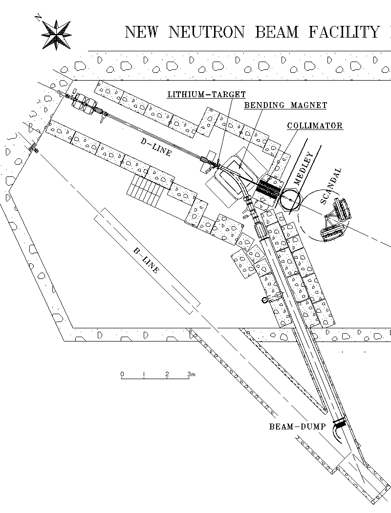
Figure 3.1: Drawing of the new neutron beam facility in the Blue Hall at TSL

The actual beam is defined by a collimator, consisting of 100 cm long iron cylinders of different diameter, embedded in a wall of concrete. These cylinders can give a beam of, more or less, any shape and diameter up to 30 cm, even though the standard forms available are circular beams in steps of about 5 cm. Right after the collimator is the experimental area with the MEDLEY setup, that is used for experiments concerning neutron-induced charged particle production and will be described in more detail in section 3.2. It is centered at a distance of 3.74 m from the lithium production target. After MEDLEY there is another setup called SCANDAL [27] used for experiments on elastic neutron scattering. Running several experiments at once like this is possible since almost the entire neutron beam passes the first setup without interacting. Two more independent neutron monitors are available namely the ionization chamber monitor (ICM) that uses the ionization of the gas inside the detector and via an electric field collects the ion pairs created [28], and the thin-film breakdown counter (TFBC) [29]. The exit area from the collimator as well as the ICM and the TFBC can be seen in figure 3.2. However, in this experiment there was a problem with the ICM so that it could not be used as an absolute monitor of the neutron flux, but instead as a relative monitor calibrated to the TFBC.

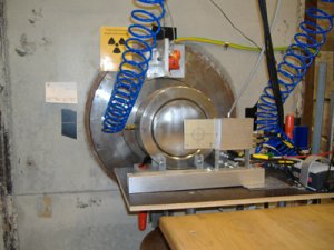
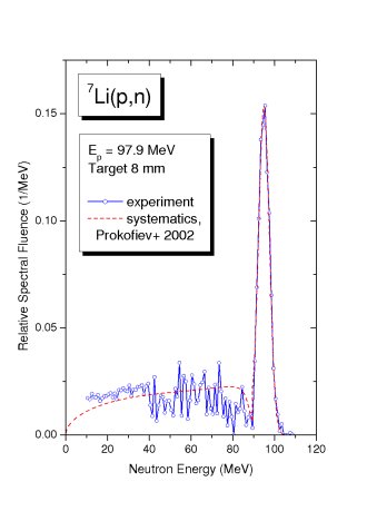
Figure 3.2: In the left panel, the exit of the collimator with the larger cylindrical ICM and the smaller rectangular TFBC in front. The right panel shows the neutron spectrum emerging from the collimator [30].

3.2 MEDLEY spectrometer

The MEDLEY spectrometer, as seen in figure 3.3, consists of a 24 cm high cylindrical vacuum chamber with 90 cm diameter. Inside this chamber there are eight telescopes mounted at even intervals covering angles from 20 to 160 degrees, four on each side, and can be changed by rotating the table inside the chamber. The distance from the target to the different telescopes can also be varied.

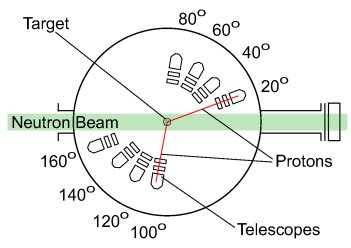
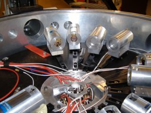
Figure 3.3: The MEDLEY spectrometer. The left panel shows a schematic sketch of the scattering chamber and in the right panel is a photography of a similar setup.

To get a clean positioning of the target within the beam without getting too much background signal from the target holder, a small aluminum frame is used that is well off the beam. The target itself is strung up in the frame using thin wires. This setup can be seen in figure 3.4. There are three of these frames so one can easily switch between targets without breaking the vacuum. For calibration purposes an ²⁴¹Am source is also available, though this was not used in this experiment.

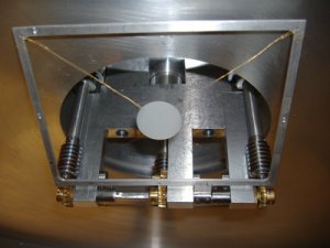
Figure 3.4: One of the aluminum frames and the CH₂ target stinged up inside the MEDLEY spectrometer.

3.3 Detector telescopes

Each of the telescopes, as can be seen in figure 3.5, in the MEDLEY spectrometer consists of three individual detectors. First there are two silicon detectors, one thin of about 50 - 60 µm and one thick of about 400 - 500 µm thickness respectively. Finally there is a 5 cm long crystal of thallium activated cesium iodide (CsI(Tl)). These detectors are often referred to as the $\Delta E_{1}$, the $\Delta E_{2}$, and the $E$ detector, or sometimes A, B, and C detector. The detectors are mounted in an aluminum housing. Since the configuration of the detectors in this experiment was not the usual for MEDLEY it is listed in table A.1.

There also exists a possibility to use plastic scintillators mounted as active anti-coincidence collimators to discard the signals from particles that did not pass straight into the detector. Attempts have actually been made in earlier experiments, but due to problems with them they were not used in this experiment.

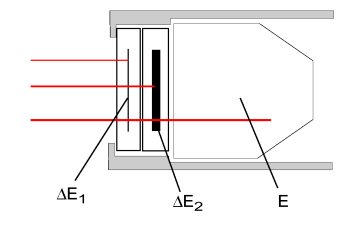
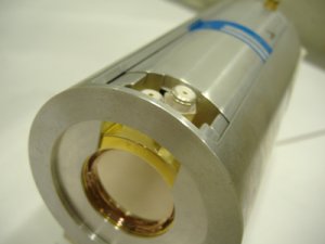
Figure 3.5: One of the detector telescopes. The left panel shows a schematic sketch of the telescope as well as the different kinds of events mentioned in section 3.3.1 and in the right panel is a photography of a similar telescope.

3.3.1 Silicon detectors

The two most common semiconductor detectors are silicon and germanium detectors, and are in principle a large diode in reverse bias. The primary way of energy loss is via Coulomb interaction in the material where the atoms are either ionized or excited. This will create electron-hole pairs that can be collected by two electrodes and measured as a small current pulse when a particle is passing through.

Another feature that is fundamental for this experiment is that the amount of energy lost per unit length is not constant. Actually it decreases with increasing energy. In figure 3.6 the stopping power and the distance a proton can travel before it is completely stopped, the so called range, is plotted for the range of proton energies relevant in this experiment. This property will be used for particle identification in the analysis.

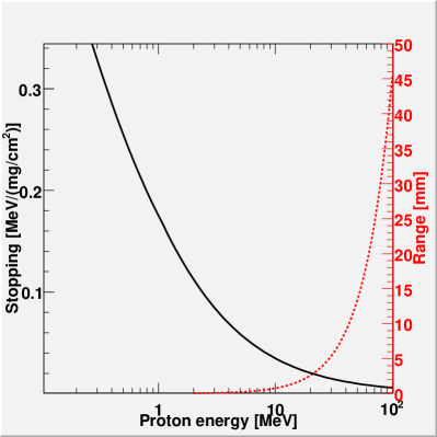
Figure 3.6: Stopping power (solid line) and range (dashed line) of protons in silicon calculated using SRIM.

These detectors are standard fully depleted surface-barrier detectors from ORTEC [31] were the silicon wafer is glued to a metal ring. One side is covered with a thin layer of gold and the other with aluminum [32]. The $\Delta E_{1}$ detector is used as a transmission detector, that is the particles pass through the detector leaving only a fraction of its energy. This is also the case for the $\Delta E_{2}$ detector at energies above 10 MeV, but for low energy events the proton is stopped in this detector. Protons that stop in $\Delta E_{1}$ are below the cutoff and are not included in the analysis. For an illustration of the different kinds of events, see figure 3.5.

3.3.2 CsI(Tl) detectors

An inorganic scintillator is used as $E$ detector in this setup. Here the incoming radiation creates electron-hole pairs in the crystal by moving an electron from the valence band to the conduction band on its way through the crystal. In the crystal, some impurities are often added. These impurities will have lower ionization energy than the crystal, which is why the holes will drift here and ionize the impurities. The ionized impurities will then pick up an electron from the conduction band and decay to the ground state and emit a scintillation photon [28].

A quite popular inorganic scintillator is the cesium iodide, available with both thallium and sodium activation. The high density of the CsI(Tl) gives it large stopping power and it also has a really high light yield of about 65000 photons/MeV [28]. The wavelength of the emission light, 540 nm, is quite bad suited for a photomultiplier tube so instead a Hamamatsu photodiode is used [31]. To suite this, the last 2 cm of the 4 cm diameter cylinder is tapered off to 1.8 cm to fit the surface of the diode. Another useful feature of the CsI(Tl) worth mentioning is that it has a variable decay time for different kinds of particles [28] that makes it suitable to use with pulse shape analysis.

3.4 Readout and electronics

Both the $\Delta E_{1}$ and the $\Delta E_{2}$ detector can generate a trigger signal, in order to allow triggers from both low- and high-energy particles. The signal from the detector is split up in two branches, a timing branch and an energy branch. A complete scheme is found in figure 3.7.

A signal from a detector is first amplified and then, if the pulse height is enough, converted to a logical signal using a constant fraction discriminator (CFD). The timing signal is split up into two branches. One of them is connected via a fan-in/fan-out (FIFO) logic to the other detector and telescopes as a master event. The other branch is delayed and sent as a stop signal for the timing channel in the time-to-digital converter (TDC). If the computer is busy processing earlier event the current event is discarded, otherwise it, through a logic FIFO, generates an energy gate signal for the analog-to-digital converter (ADC) and charge-to-digital converter (QDC) units, a start signal for the TDC and finally a trigger for the data acquisition.

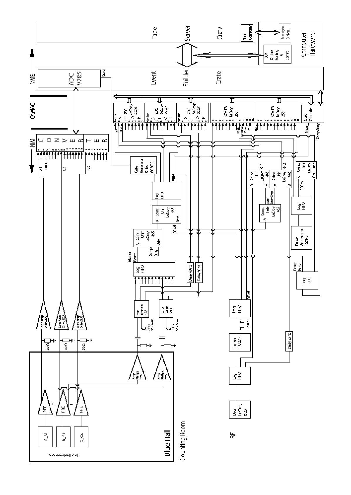
Figure 3.7: Scheme of the MEDLEY electronics as of week 9, 2004

The energy signal is recorded from all three detectors and all eight telescopes as soon as one detector triggers. It is sent into a ADC, with the previously named master signal as gate, after amplifying and shaping. From the cyclotron one also gets a RF signal that indicates a pulse from the neutron beam. The RF is split up through a FIFO into three branches. Two of the RF signals, where one is delayed, are used as a stop signal for the time-of-flight (TOF) channels in the TDC. It is also possible to use this RF signal as a veto for the master signal if the cyclotron is switched off.

3.5 Data acquisition

For the data acquisition a system called SVEDAQ is used, and it is summarized here from [34]. The system is taken from the EUROGAM experiment and has been modified to be suitable for use at the TSL. It is divided into three main blocks, as can be seen in figure 3.7, connected via two independent networks. The three blocks are the event builder, the tape server and the control and monitoring workstation.

The event builder is the block that reads out the data from the ADC units in the VME crate as well as the TDC units and scalers in the CAMAC crate. The event builder itself is also located in the VME. It mainly consists of a Motorola CPU that runs the readout program and sends packages to the data network when the readout buffers are full. It also sends the computer busy signals for vetoing of the master event and the 100 Hz clock so that events occurring during processing of other events are discarded.

The tape server is an optional part of the acquisition system. Of course if one wants to use the data after the experiment one needs to write it to the hard drive, but if one wants to conduct different kinds of test runs it is not needed by the event builder.

To control all this a SUN workstation is used. It is via this workstation that the system is started and stopped, but since the three blocks are more or less independent of each other the event builder and tape server will continue to write data from the CAMAC and VME even if the workstation is completely shut down. This workstation is connected to the local area network at TSL and can be remotely controlled from there. But it is also connected to the data network via a sort-spy daemon process so it can listen to the traffic without formally being a part of the network with its own IP number. This makes it possible to display a large number of one- and two-dimensional spectra from the CAMAC signals and conduct some on-line sorting and analysis.

4 Data analysis

The analysis of the data is split up into several parts. Since the SVEDAQ system writes the events as binary data, the raw files first have to be properly decoded. After the decoding, the information needs to be calibrated so that it corresponds to correct energy and timing information, before the particle selection procedure can take place, where events corresponding to the right particle type and incoming neutron energy are selected. Finally the relevant corrections for background and other effects can be carried out before extracting the final cross section.

During the analysis, three different data sets were analyzed simultaneously. Two of them were the calcium data and the background data, while the third was a reference data set of polyethene for calibration and normalization purposes. The complete set of runs is listed in tables A.2 and A.3.

4.1 ROOT

The main tool used for the analysis is ROOT. ROOT is an object oriented data analysis framework initiated at CERN by René Brun and Fons Rademakers. The framework is freely distributed as open source, where everyone is free to further distribute and modify it. This is something that has contributed, and still is contributing, to its rapid growth. It contains a large amount of packages concerning different part of data analysis like histogramming, curve fitting, minimization, statistics tools and much more [35].

The framework of ROOT is closely bound to a C++ interpreter called CINT that is written by Masahuru Goto. This means that one actually can use C++ as a scripting language for rapid prototype development of programs. Then the same code can be compiled to take advantage of the fast running of a machine language executable, unlike if one had used a normal scripting language like Ruby, Perl or Python for the prototyping.

4.2 Decoding

The raw data from SVEDAQ are written into binary data files in the EUROGAM standards with a 24 byte header followed by event-by-event records [34]. A typical example of a data sequence can be found in figure A.2. The events are recorded as a series of shorts, with the first one being the number of bytes that are used to register one event. Between the first short and the telescope events there are 20 scaler channels with numbers 1-13 containing information about the telescope triggers, the 100 Hz clocks and the neutron monitors. The last seven channels are left empty. Next is the telescope events, each of them written in five shorts corresponding to three energy signals, one from each detector, and timing signals from the two silicon detectors. Finally the two RF signals are written before the event is ended. To translate the SVEDAQ files into ROOT files a small computer code called SV2ROOT [36] was used.

4.3 Calibration

4.3.1 Energy calibration

Since the data from the runfile are given in the unit of channel numbers from the ADC an energy calibration is needed to convert these to incoming energies. The silicon detectors are assumed to have a linear response to the energy, that is the correlation looks like

$$E=kx+m$$ (4.1)

where $E$ is the energy output, $x$ is the channel number, and $k$ and $m$ the constants to be fitted.

Unfortunately the CsI(Tl) is not that simple since it has a non-linear response function between light output, $L$, and incoming energy, $E$, which makes the calibration more complicated. The light output is assumed to be given by a three-parameter formula that follows

$$L=a_{0}+a_{1}\left(E-a_{2}Az^{2}\ln\left[\frac{E+a_{2}Az^{2}}{a_{2}Az^{2}}\right]\right),$$ (4.2)

where $a_{i}$ is the fitting constants, and $A$ and $z$ is the mass number and charge of the incident particle [31]. However, to conduct the calibration we need the inverse of expression (4.2). Since this inverse is analytically complicated to calculate, the approximation according to Dangtip et al. [31]

$$E\approx a+bL+c(bL)^{2}$$ (4.3)

is used for the hydrogen isotopes. The parameter $c$ depends only on particle type and is found by Tippawan [12] to be $c=0.0032$ for protons, which leaves only $a$ and $b$ as constants to be fitted.

Here the calibration of the silicon detectors is done by calculating the incoming energies needed to break through each of the silicon detectors - the punch through energies. These are calculated using a program called The Stopping and Range of Ions in Matter (SRIM), based on the work of Ziegler et al. [37]. The punch through values for Telescope 1 (T1), Telescope 2 (T2), Telescope 7 (T7) and Telescope 8 (T8) are found in table 4.1.

	T1		T2		T7		T8
	$\Delta E_{1}$	$\Delta E_{2}$	$\Delta E_{1}$	$\Delta E_{2}$	$\Delta E_{1}$	$\Delta E_{2}$	$\Delta E_{1}$	$\Delta E_{2}$
Thickness [µm]	64.9	549	60.5	538	52.9	424	61.6	550
p [MeV]	2.42	8.62	2.32	8.51	2.34	8.63	2.13	7.41
d [MeV]	3.12	11.5	2.99	11.4	3.02	11.5	2.74	9.87
t [MeV]	3.60	13.5	3.43	13.4	3.47	13.6	3.14	11.6
3He [MeV]	8.60	30.6	8.23	30.2	8.32	30.6	7.56	26.3
4He [MeV]	9.56	34.4	9.14	34.0	9.24	34.5	8.38	29.6
6Li [MeV]	18.1	65.3	17.3	64.6	17.5	65.4	15.9	56.3
7Li [MeV]	19.1	69.7	18.3	68.9	18.5	69.8	16.7	60.0

Table 4.1: Thickness and punch through energies for the different silicon detectors used.

If one plots the $\Delta E_{1}$ versus $\Delta E_{2}$, these punch though points manifest themselves as turning points in the particle bands as can be seen in the left panel of figure 4.1. It is now quite straightforward to compare the channel numbers of these areas to the values in table 4.1 and get the coefficients to (4.1).

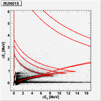
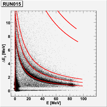
Figure 4.1: Calibrated $\Delta E_{1}$-$\Delta E_{2}$ and $\Delta E_{2}$-$E$ plots for T1. The red lines correspond to tabulated energy loss values for protons, deutrons, tritons, ³He and alpha particles in ascending order. The apparent mismatch for some lines in the right panel is due to the non-linear effects in the CsI(Tl).

But once again, the CsI(Tl) poses a bit of a problem. As can be seen in the right panel of figure 4.1, there are no turning points available for calibration. Instead, at least in forward angles, one can use the quite strong peak of elastic p(n,p) scattering in the CH₂ runs as one calibration point. In the lower part of the $E$ scale the proton band is quite bent, so here a couple of points are selected and the energy deposited in the $E$ detector is calculated from the energy lost in $\Delta E_{2}$. Numerical values obtained for the calibration constants are listed in table A.4.

4.3.2 Time calibration

For the time calibration a couple of special runs devoted were made. During these runs cables of different lengths, giving different delay times, were put between the RF signal and the TDC, displacing the peak in the recorded RF signal. The result from these runs can be fitted with a linear calibration formula

When each of the RF signals are time calibrated they need to be combined into a single time line. The two RF signals can be plotted against each other in figure 4.2, where four areas can be identified, schematically illustrated in figure 4.3. Events in area 1 and area 3 are events that occur during one of the RF signal pulses, and hence get start and stop signals simultaneously. So in these areas we only get signal from one of the RF. In area 2 and area 4 there is a signal from both RF 1 and RF 2.

To translate the two RF signals into a single time scale, one of the RF signals is chosen as base, in this case RF 1. In the areas where no information exists for the chosen base RF signal, the information from the other RF signal is transformed to the chosen base according to the algorithm in [33].

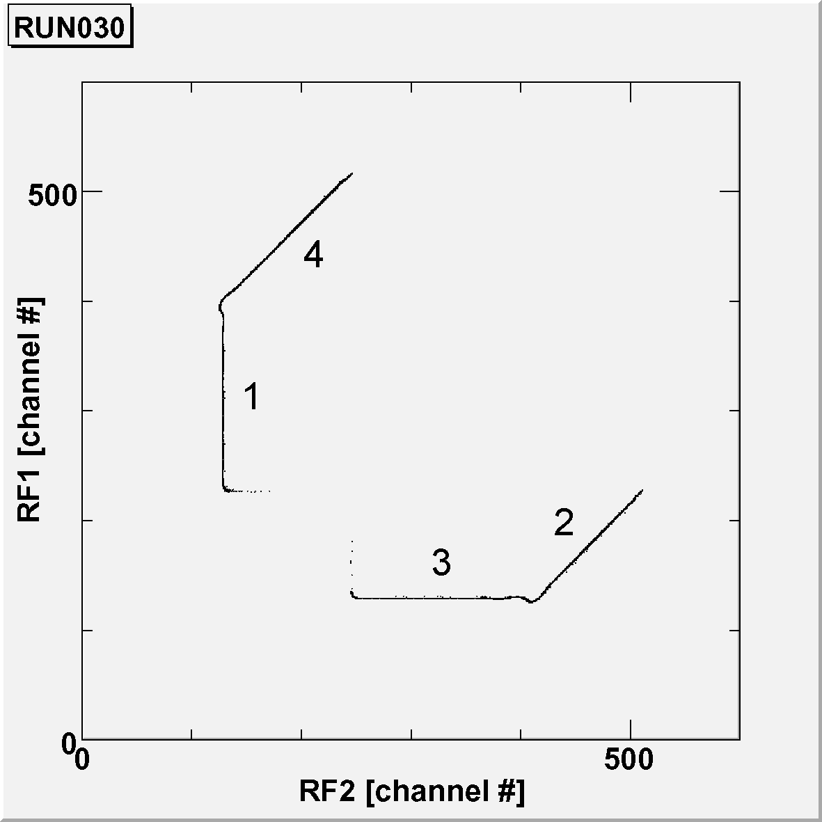
Figure 4.2: RF 1 versus RF 2. Each point in the 8-shaped trajectory correspond to a time between detection and production of the next burst. One lap around is 58 ns.

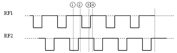
Figure 4.3: Scematic illustration of the two RF signals and the different possible events that can occur [33]. The RF is measured as the from the trigger to the next signal from the cyclotron.

4.4 Particle identification

As mentioned earlier, the bands that are shown in figure 4.1 correspond to different kinds of charged particles. This makes the particle identification procedure quite straightforward by taking some rough cuts around the structures of the desired particle type. These cuts should be very generous, since it is always easier to remove unwanted events than to recreate wanted ones and is shown for T1 in figure 4.4. The criterion here is that an event must be in both of these to be selected.

Figure 4.4: First graphical selection cuts for protons in T1. In the left panel the cut for the $\Delta E_{1}$-$\Delta E_{2}$ plot is shown and in the right panel the $\Delta E_{2}$-$E$ plot is shown.

When these first rough cuts are done, the particle bands are straightened for a more refined selection of events. To do this, the energy recorded in the $E$ detector is used together with SRIM to calculate the corresponding energies in the $\Delta E_{1}$ and $\Delta E_{2}$ detectors. By subtracting this value from the energy actually recorded the particle bands are straightened out around zero. The $\Delta E_{1}(\textrm{exp})-\Delta E_{1}(\textrm{tab})$ selection is mainly used to remove noise in the low energy region in the $\Delta E_{1}$-$\Delta E_{2}$ plot, and the $\Delta E_{2}(\textrm{exp})-\Delta E_{2}(\textrm{tab})$ selection is used to get a cleaner separation between protons and deuterons. These two are shown in figure 4.5.

Figure 4.5: Refined selection cuts for protons in T1. In the upper left panel the cut for the $\Delta E_{1}(\textrm{exp})-\Delta E_{1}(\textrm{tab})$ plot is shown and in the upper right panel the $\Delta E_{2}(\textrm{exp})-\Delta E_{2}(\textrm{tab})$ plot is shown. The lower panels contains the final proton cuts as in figure 4.4 for T1 together with the tabulated curve from SRIM

4.5 Time-of-Flight measurements

When only protons are selected, the next restriction is to only select protons that are produced by neutrons of the correct energy. Since the neutron beam is not completely monoenergetic, but contains about 60 % lower energy neutrons [31], the contribution from these has to be removed. To do this the TOF information obtained in section 4.3.2 is used. The TOF, $t$, for a particle with energy $E_{k}$ and velocity $v$ to travel a distance $s$ can be calculated as

$$t=\frac{s}{v}.$$ (4.4)

The velocity of the particle is given in its rest mass, $m_{0}$, and its momentum, $p$, as

$$v=\frac{p}{\sqrt{m_{0}^{2}+\frac{p^{2}}{c^{2}}}}$$ (4.5)

where the $p$ is given by

$$p=\frac{1}{c}\sqrt{E_{k}^{2}+2E_{k}m_{0}c^{2}}.$$ (4.6)

Plugging (4.6) into (4.5) into (4.4) and simplifying yields

$$t=\frac{s}{c}\sqrt{\frac{(m_{0}c^{2}+E_{k})^{2}}{E_{k}(E_{k}+2m_{0}c^{2})}}$$ (4.7a)

$$E_{k}=\sqrt{m_{0}^{2}+\frac{m_{0}^{2}}{\left(t\frac{c}{s}\right)^{2}-1}}-m_{0}$$ (4.7b)

where Eqs. (4.7a) and (4.7b) are equivalent.

But the time scale mentioned in section 4.3.2 includes both the neutrons TOF as well as the charged particles TOF from the target to the telescope. As can be calculated from (4.7a), if the particle is a 94.5 MeV neutron traveling a distance of 3.74 m the TOF would be about 29.9 ns. A 5 MeV proton traveling 26.83 cm has a TOF of 8.71 ns while a 90 MeV proton would have a TOF of only 2.19 ns. This makes quite a large difference, especially at low energies, and is compensated for by subtracting the charged particle TOF, calculated from the energy of $\Delta E_{1}$, $\Delta E_{2}$ and $E$ added together. The final TOF cuts are illustrated in figure 4.6.

Figure 4.6: Neutron TOF versus proton energy for calcium in the left panel, and CH₂ in the right panel, together with the TOF cut. The the low energy tail in the neutron spectra is clearly visible in the CH₂ plot. The extra TOF cut at high energies is motivated in section 6.3.

To choose a suitable sized cut, the elastic p(n,p) scattering is chosen to define the width. This peak has a full width at half maximum (FWHM) of 6.6 ns, quite in agreement with Dangtip et al. [31] where the FWHM is measured to be about 6-7 ns, and one of the large contributions is the finite time of a beam pulse from the cyclotron. The with of the cut is chosen as two standard deviations, and is a compromise between statistics, minimizing mismatching errors, and a high lower limit of the accepted neutron spectrum. For more details, see section 6.4.

4.6 Corrections

For each run, the live time of the data acquisition system is corrected for. As mentioned in section 3.4, events that occur while an earlier event is treated are discarded. The amount of discarded events is not constant, as seen in figure 4.8, but is assumed to be. The ratio of discarded events is obtained by comparing the 100 Hz scaler and the 100 Hz computer busy scaler. The finite efficiency of the CsI(Tl) is also corrected for. This has a non-linear dependence of energy deposited, and this is simulated by both MCNPX and GEANT [38]. The results of these simulations are found in figure 4.8. Since they are in good agreement, one of them is choosen, in this case the GEANT results.

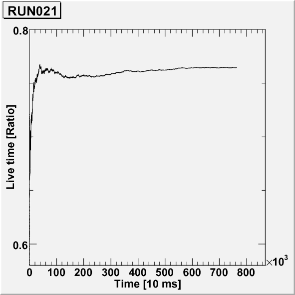
Figure 4.7: Typical live time of a run. The instabilities in the beginning are due to statistics.

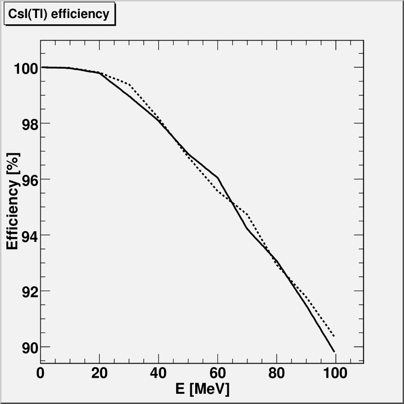
Figure 4.8: Efficiency of the CsI(Tl) detector. The dashed line is a simulation with MCNPX and the solid line is a simulation with GEANT [38].

During the entire event-by-event analysis, the data sets from the runs containing an empty frame were treated in parallel to the calcium and the polyethene data. When switching to analysis of histograms instead of events, the data from the background runs kan be subtracted from the calcium and polyethene data. In that way one can get pure signal histograms. A comparision between the calcium, polyethene and background data can be found in figure 4.9. The background in MEDLEY has been analyzed thoroughly by Tippawan [12] for the old facility. Its main components are particles produced by produced neutrons reacting in the beam pipe and the reaction chamber, and the CsI(Tl) and the telescope housing acting as an active target for the beam halo.

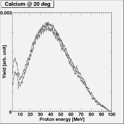
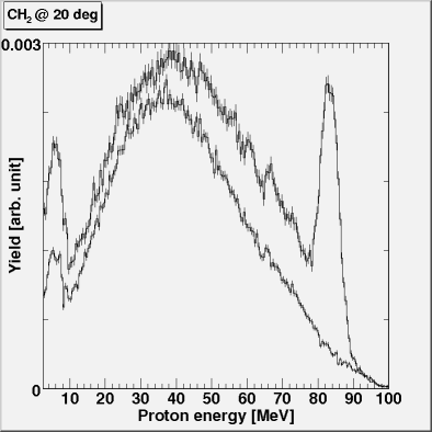
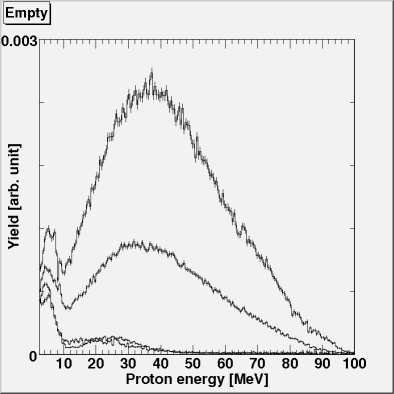
Figure 4.9: In the top panels, the signal and background for calcium, left, and polyethene, right, at an angle of 20 degrees. The bottom panel shows the background for the four angles analyzed: 140 degrees, 160 degrees, 40 degrees and 20 degrees in increasing order.

4.6.1 Target thickness

To achieve a count rate that is acceptable, some demands are put on the target. Since the neutron beam is quite low in intensity and only a small fraction of the neutrons interacts the target has to have some finite thickness. For high-energy protons this is of negligible importance. For low energy protons, on the other hand, the energy loss can be quite significant. In table 4.2, SRIM calculations for low energies are shown to illustrate the problem. The target used in these measurements was about 230 $\mu$m thick. These effects are compensated for through a method implemented in a computer code, TCORR, by Pomp and Tippawan [39] and is based on iterative calculations of response functions. The result of the target correction procedure is found in figure 4.10.

Ion Energy [MeV]	$\textrm{d}E/\textrm{d}x$ [keV/$\mu$m]	Range [$\mu$m]	Straggling [$\mu$m]
3.25	11.854	164.35	7.51
3.50	11.247	185.84	8.35
3.75	10.708	208.46	9.19
4.00	10.225	232.18	10.06
4.50	9.3934	282.85	12.85
5.00	8.7004	337.80	15.54
5.50	8.1137	396.92	18.20
6.00	7.6086	460.15	20.86
6.50	7.1698	527.41	23.55

Table 4.2: Stopping of protons in calcium

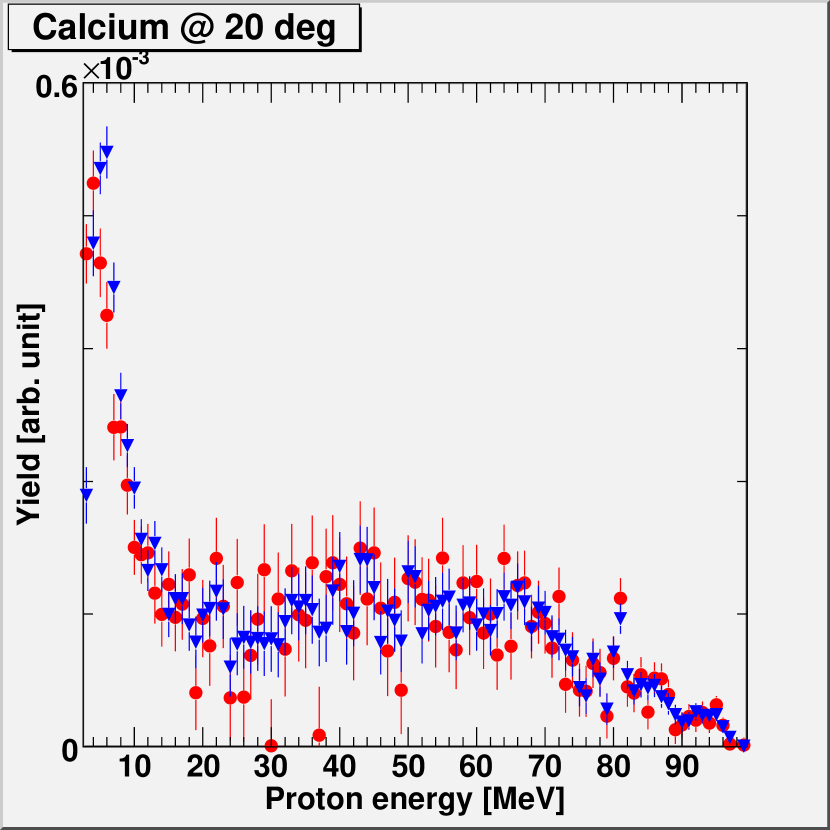
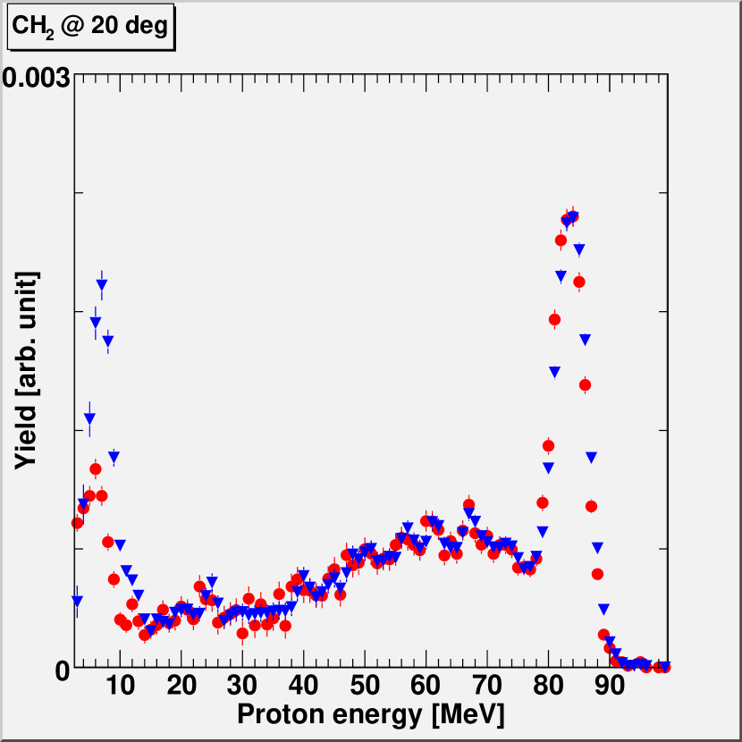
Figure 4.10: Target correction results for calcium in the left panel and polyethene in the right panel. Red circles represent the original data, while blue triangles show the corrected data, re-binned to 1 MeV for comparison. After three iterations the Kolmogorov test gave 100% probability for the current iteration compared to the previous one.

4.7 Accepted neutron spectrum

Even with the TOF selection in section 4.5, not all low energy neutrons were rejected. As can be seen in figure 4.6 the finite width of the TOF cut results in events induced by neutrons down to around 60 MeV to be accepted. In the same figure one can also see the how the low energy p(n,p) tail wraps around the time scale and allows events by about 10-14 MeV neutrons inside the cut. To be able to subtract data originating from these events the accepted neutron spectrum is deduced from the CH₂ data. To get a clean neutron spectrum, the contribution from carbon has to be subtracted from the CH₂ data. For 95 MeV neutrons, the subtracted carbon cross section comes from existing experimental data [24]. This is not possible for lower energy neutrons, so their contribution to the carbon spectrum is taken from tabulated data in [40].

To obtain a p(n,p) spectrum, the peak at 83 MeV is normalized to a cross section obtained from the partial wave analysis (PWA) solution SP05 of [41] via a procedure described in appendix B. In this first normalization, the fact that also carbon contributes slightly to the peak is ignored, but the peak is re-normalized to the cross section from [41] after the subtraction of experimental carbon data.

Now the remaining CH₂ data are divided into bins corresponding to 10 MeV neutron energy each, translated to elastically scattered proton energies as seen in table A.5. The bin right below the peak is integrated and the number of events in the bin is corrected for the variation in p(n,p) cross section, also listed in table A.5. The cross section is assumed constant within the bin and equal to the cross section in the center of the bin. When doing this an assumption is made that the high Q value of the C(n,p) reaction makes the contribution from the carbon to the bin content negligible. Now, when one have the fraction of accepted neutrons in that bin compared to the full energy peak, one can subtract the corresponding carbon cross section obtained from [40]. In parallel, the obtained bin content relative to the peak is used to build up an accepted neutron spectrum. This process is then iterated downwards in energy for each of the bins until a pure p(n,p) spectrum and a corresponding neutron spectrum is available, and the resulting spectrum is found in figure 4.11 and in table 4.3.

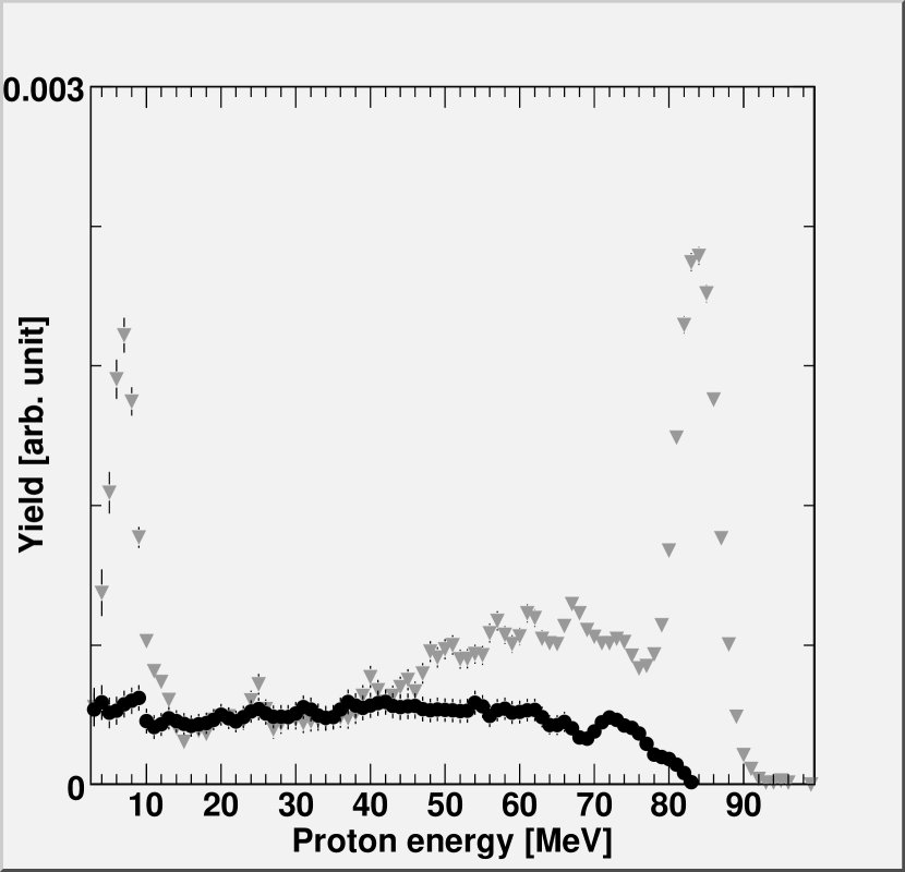
Figure 4.11: The deduced pure np spectrum in the left panel. Grey triangles are polyethene data and black circles are carbon data from the procedure in section 4.7. In the right panel is, the fraction of accepted neutrons per bin is shown.

Bin [MeV]	Contribution [%]
5-15	3.2
15-25	0
25-35	0
35-45	0
45-55	0
55-65	6.9
65-75	10
75-85	17
85-100	61

Table 4.3: Accepted neutron spectrum, as seen in figure 4.11.

4.8 Normalization

To obtain a value for the cross section all data are normalized to elastic p(n,p) scattering at 20 degrees. This since the p(n,p) scattering cross section is well known and the peak is clear at this angle. The peak together with a gaussian fit is seen in figure 4.12.

Figure 4.12: The elastic np peak fitted with a gaussian. The data are CH₂ with carbon [24] subtracted.

The FWHM of the peak is found to be 6.4 MeV, in agreement with the FWHM in Dangtip et al. [31], with the solid angle of the telescope as the main contribution. The cross section, $\sigma$, for each bin, $i$, in telescope $\textrm{T}X$ is now calculated from

$$\frac{\sigma_{\textrm{Ca},i,\textrm{T}X}}{N_{\textrm{Ca},i,\textrm{T}X}}=\frac{\sigma_{\textrm{H}}}{N_{\textrm{H}}}\frac{2m_{\textrm{CH}_{2}}}{M_{\textrm{CH}_{2}}}\frac{M_{\textrm{Ca}}}{m_{\textrm{Ca}}}\frac{\Omega_{\textrm{T}1,\textrm{T}8}}{\Omega_{\textrm{T}X}}\frac{\Phi_{\textrm{CH}_{2}}}{\Phi_{\textrm{Ca}}}$$ (4.8)

where $N$ is the number of counts, $m$ is the target mass, $M$ is the molecular mass, $\Phi$ is the relative neutron flux and $\Omega$ is the solid angle. Since the target distances for T1 and T8 are the same, as seen in table A.1 the solid angles for these telescopes are assumed to be equal. The other six telescopes, as also seen in table A.1 however needs to be corrected with a factor of 0.546, from a simple geometrical point of view. For a more in-deep analysis of the solid angle in MEDLEY, see [42].

Since the polyethylene is the reference target that is regularly used in MEDLEY experiments the weight, and number of protons, has been measured with high precision to be $461.55\pm 0.01$ mg and $3.963\cdot 10^{22}$ protons [42]. The weight of the calcium target used was measured to be $235.9\pm 0.1$ mg before the runs and $237.3\pm 0.1$ after the runs, which averages to 236.6 mg.

The cross section, $\sigma_{\textrm{H}}^{\textrm{cm}}$, is taken from Rahm et al. [43] where the p(n,p) cross section at a center of mass (CM) angle of 139.0 degrees and at 96 MeV is measured to be 7.735 mb/sr. In order to extrapolate this to 94.5 MeV at a CM angle of 139.1 degrees, data from PWA solution SP05 are used. From [41] the cross section for 94.5 MeV and 139.1 degrees is 8.041 mb/sr, while the cross section for 96 MeV and 139.0 degrees is 7.928 mb/sr. This gives an increase in cross section of about 1.43 %. Via the procedure in section B this is translated into $\sigma_{\textrm{H}}^{\textrm{lab}}=30.53$ mb/sr.

5 Results

The results given here are those of the accepted neutron spectrum obtained in section 4.7 and listed in table 4.3, resulting in a mean value for the neutron energy of 79.7 MeV. The total cross section for this spectrum is found in table A.12 with a cutoff energy of 2.5 MeV.

5.1 Double-differential cross sections

Double-differential cross sections at four different angles have been analyzed. The result is found in figure 5.1 and tables A.6-A.9, which also include corrected data introduced in section 6.1.3.

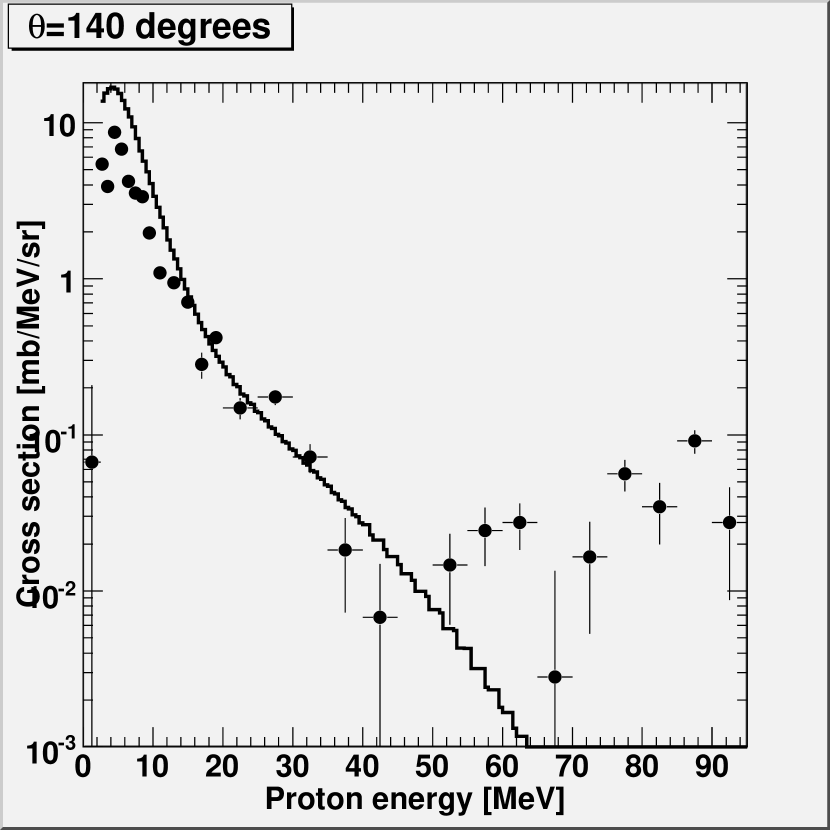
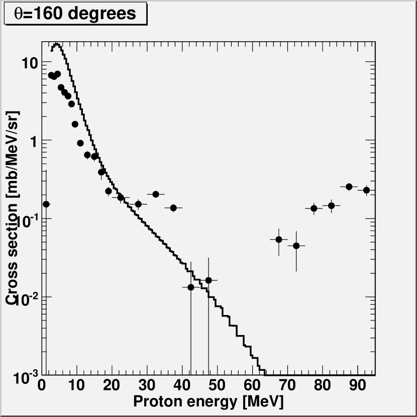
Figure 5.1: Experimental double-differential cross sections, filled circles, for the neutron spectrum in table 4.3 in the Ca(n,px) reaction. The solid histogram is TALYS calculations for this neutron spectrum. Cutoff energy is 2.5 MeV.

5.2 Single-differential cross sections

5.2.1 Angular-differential cross section

To get angular-differential cross sections, the double-differential spectra are summed over and weighted for the different bin widths. The result is found in table A.11. In figure 5.2 the angular-differential cross section for bins corresponding to compound, pre-equilibrium and direct reactions is found.

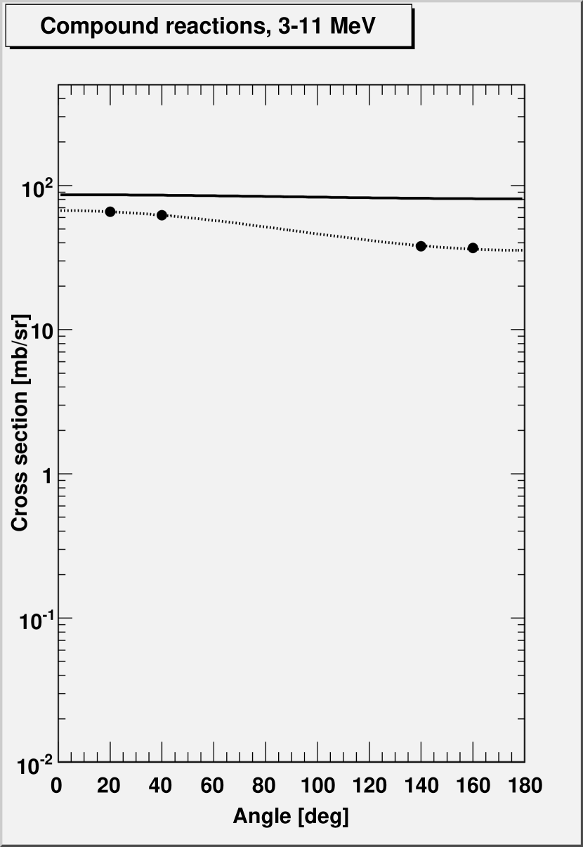
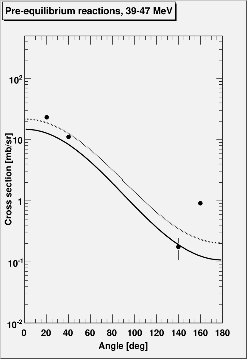
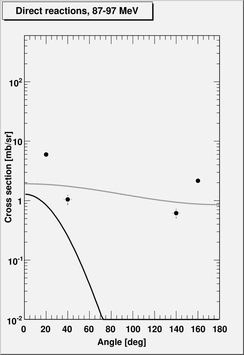
Figure 5.2: Experimental angular-differential cross sections for three different bins and the neutron spectra in table 4.3 in the Ca(n,px) reaction. The chosen bins are assumed to represent the three specific reaction types. The solid line results from TALYS and the dotted line is a fit to the data according to Eq. (2.11). Cutoff energy is 2.5 MeV.

5.2.2 Energy-differential cross section

To get energy-differential cross sections, each of the energy bins in the double-differential spectra are fitted with Eq. (2.11). Using the results from this fit, the data are interpolated to the angles 60, 80, 100 and 120 degrees, and also extrapolated to 5 and 175 degrees. These data points are summed over and weighted for the different bin as well as their angular contribution. The result is found in figure 5.3 and in table A.10.

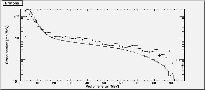
Figure 5.3: Experimental energy-differential cross sections, filled circles, for the neutron spectrum in table 4.3 in the Ca(n,px) reaction. The solid histogram is TALYS calculations for this neutron spectrum. Cutoff energy is 2.5 MeV.

6 Discussion

6.1 Comparison with theory

To be able to compare the result with theoretical calculations the contribution from the low-energy neutrons need to be subtracted. To do this three different methods, listed in sections 6.1.1-6.1.3, are presented. The difference in total cross section between these methods is shown in table 6.1.

6.1.1 Method 1: Rescaling of experimental data

In the first method for subtraction of low-energy neutron data, the energy spectrum for proton emission is assumed to be independent of the incoming neutron energy. The experimental cross section is weighted with the amount of low energy neutrons in the accepted spectrum from table 4.3, and rescaled to the peak in the neutron spectrum. The result is found in figure 6.6.

The main advantage of this method is that one gets rid of the model dependencies in the TALYS calculations, and the data used are pure experimental. This means that the result at low energies, up to about 40 MeV, should be quite accurate. The main disadvantage on the other hand is the obvious fact that the cross section spectrum for 94 MeV neutrons and lower energy neutrons differ a lot at high energies. This is especially relevant at energies above the low energy bin under consideration.

6.1.2 Method 2: Subtraction of TALYS data

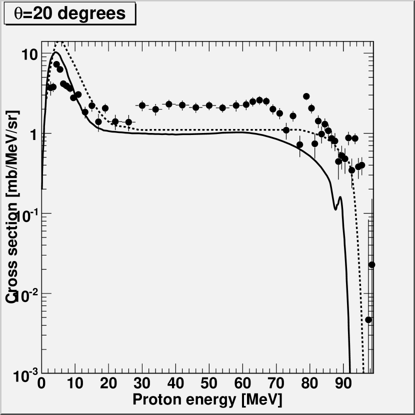
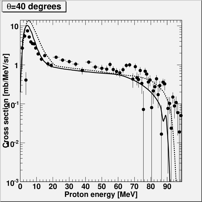
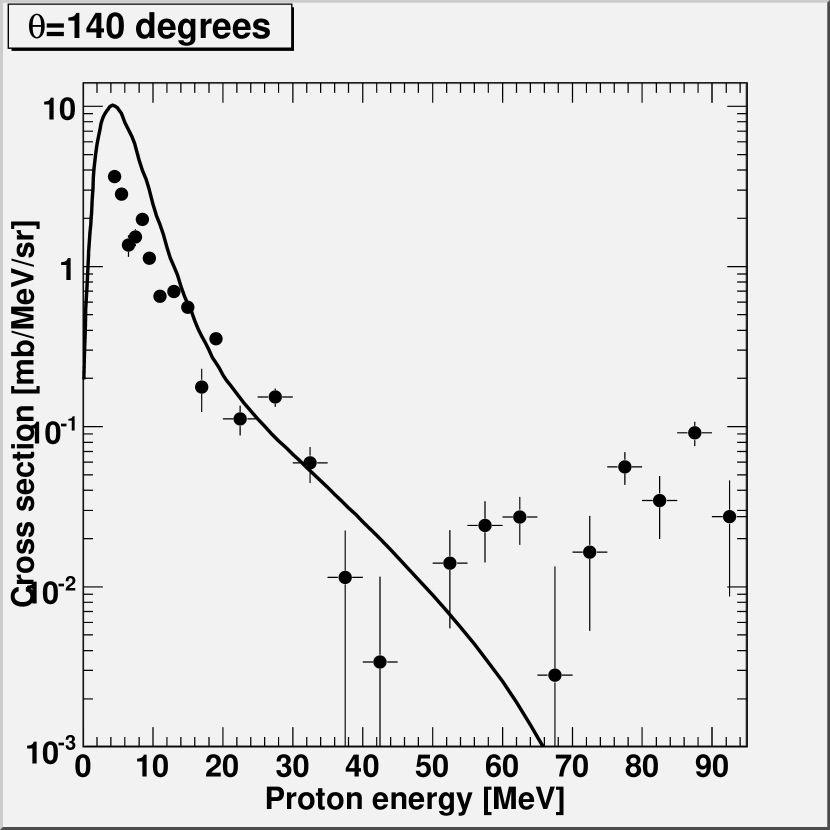
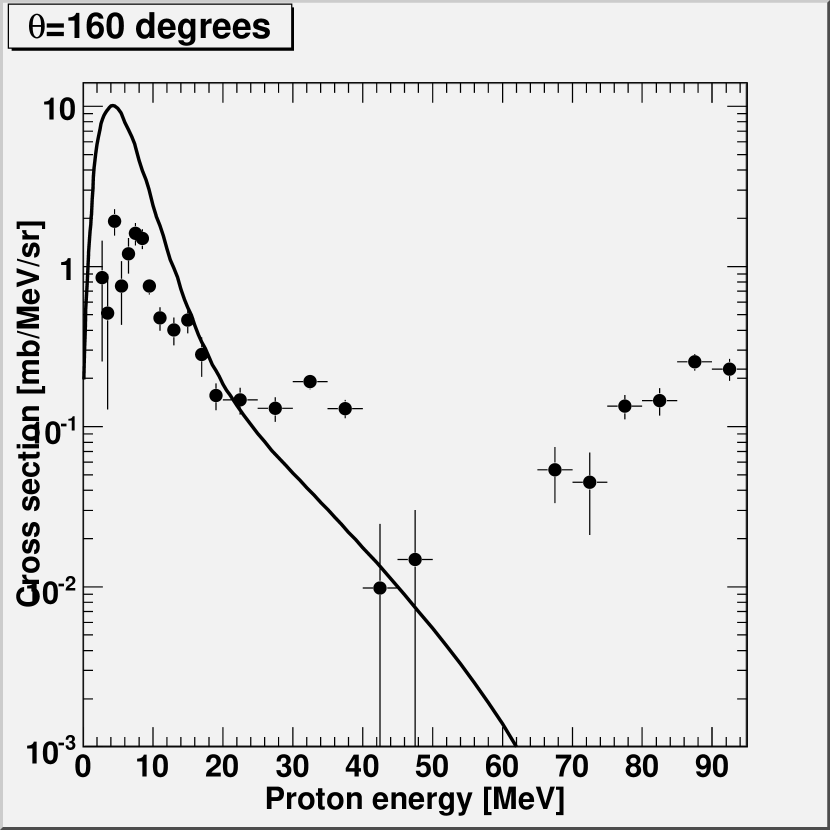
Figure 6.7: Double-differential cross sections in the four top panels, and angle integrated single-differential cross section in the bottom panel, with TALYS data (method 2) subtracted for 94 MeV neutrons in the Ca(n,px) reaction. Solid lines are predictions by TALYS, and dashed lines are predictions by GNASH [40]. Cutoff energy is 2.5 MeV.

Another way to correct for the low-energy neutron contribution is by using data from TALYS. For the accepted neutron spectrum in table 4.3, TALYS is used to calculate cross sections for each bin. The bins between 15 MeV and 55 MeV are left out, since the contribution in these bins probably derive from statistics. The result is found in figure 6.7.

The advantage of using this method is that it makes the comparison between experiment and theory straightforward. The difference one can see in figure 6.7 between experiment and theory is directly related to the TALYS calculations. So for code verification purposes, this method works fine. But for obtaining experimental data, this method is not so good, since the resulting experimental data points will have a heavy model dependency on calculations that are known to be incorrect.

6.1.3 Method 3: Subtraction of modified TALYS data

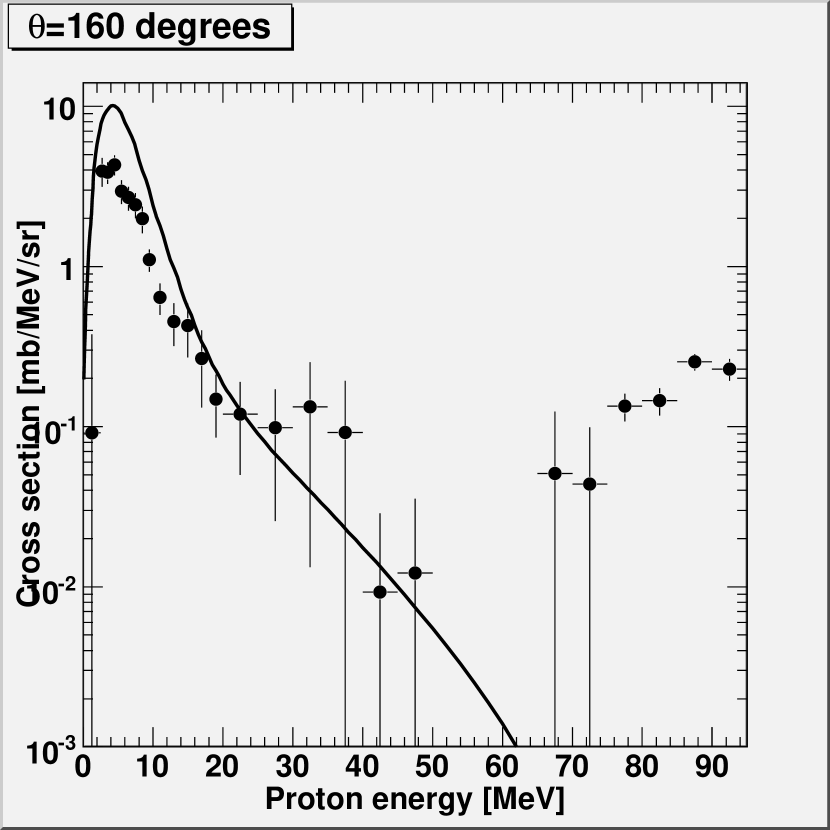
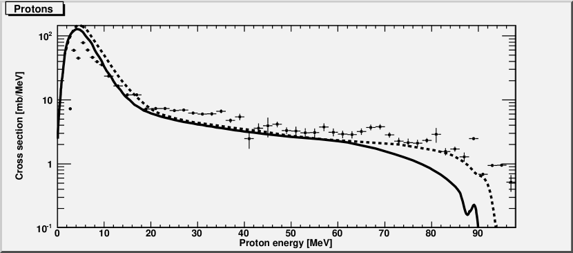
Figure 6.8: Double-differential cross sections in the four top panels, and angle integrated energy-differential cross section in the bottom panel, with modified TALYS data (method 3) subtracted for 94 MeV neutrons in the Ca(n,px) reaction. Solid lines are predictions by TALYS, and dashed lines are predictions by GNASH [40]. Cutoff energy is 2.5 MeV.

A third possible method is to try and modify the TALYS data to get it more correct. From previous experiment, TALYS is known to heavily overestimate the evaporation cross section in backward angles, and slightly overestimate it at forward angles. It also appears to underestimate pre-equilibrium cross sections in forward angles [22, 23]. Here, an assumption is made that the over/under-estimations in the TALYS calculations are truly systematic and do not vary with projectile energy. From this assumption one can divide the experimental data with the TALYS data in figure 5.1 and get a correction histogram. This correction histogram is assumed to contain the true over/under-estimations in TALYS, and by multiplying the low-energy TALYS calculations with this before subtracting them, the true cross-section spectra are obtained. The result is found in figure 6.8 and, together with uncorrected data, in tables A.6-A.9.

By using this method one can reduce the model dependencies compared to unmodified TALYS data, by adjusting the theory to the experiment. This method is the one that probably will give the result with smallest systematic errors for the low-energy neutron correction. However, it is first when one sees the results from similar experiments at different energies that one can conclude if the assumption made is too bold or not.

Method	$\frac{\textrm{d}\sigma}{\textrm{d}\Omega}(\theta=20)$	$\frac{\textrm{d}\sigma}{\textrm{d}\Omega}(\theta=40)$	$\frac{\textrm{d}\sigma}{\textrm{d}\Omega}(\theta=140)$	$\frac{\textrm{d}\sigma}{\textrm{d}\Omega}(\theta=160)$	$\sigma_{\textrm{prod}}(\textrm{n},\textrm{p}x)$
1. Exp. Data	$155\pm 2.92$	$99.4\pm 1.54$	$31.6\pm 0.486$	$32.1\pm 0.700$	$746\pm 1.97$
2. TALYS	$188\pm 4.76$	$107\pm 2.51$	$17.6\pm 0.792$	$18.6\pm 1.14$	$679\pm 3.74$
3. Mod. TALYS	$175\pm 6.69$	$107\pm 4.22$	$33.7\pm 1.73$	$35.1\pm 2.04$	$788\pm 5.83$
TALYS	131	106	62.4	62.4	1070
GNASH [40]	186	145	-	-	1300

Table 6.1: Comparison of angular-differential and total cross sections with subtracted data. Differential cross sections are given in mb/sr and total cross sections in mb. The cutoff energy is 2.5 MeV, except for the GNASH calculations of $\sigma_{\textrm{prod}}(\textrm{n},\textrm{p}x)$, where no cut-off is was applied.

6.2 Background and shielding

As can be seen in figure 4.9 the background problem is quite heavy. In the silicon data runs from the old facility, the signal-to-background ratio was about 8 [12]. By moving the spectrometer closer to the lithium target, and at the same time reducing the shielding, the background increased dramatically. In later data sets with energies of 180 MeV, the background problem were so large that it was virtually impossible to get acceptable results from the data [36]. To come to terms with the background problems recent GEANT simulations at St. Petersburg University show that the background for a 180 MeV neutron beam can be reduced by a factor 20-50, by exchanging the concrete wall to an iron wall. The background would probably be reduced even more for a 94 MeV beam. Available iron blocks from the old CELSIUS ring have actually been used when this reconstruction was undertaken in January 2007. The first data with the new shielding will probably be taken during February 2007.

6.3 Special TOF cut

Run 37 was itself unusable for the analysis, but still it may contain some interesting information on the phenomena. As can be seen in the right panel of figure 6.1 there exists a really strong shift in the TOF at high energies that does not seem to be constant, but disappears around 60 MeV. This effect is also visible in T1 as can be seen in the left panel of figure 6.1. This clear energy dependence makes a correction for this effect quite difficult. Therefore, the TOF cut instead has been expanded to include these effects. This had to be done for both T1 and T8 since the effect still was present, but weak, after the threshold adjustment in T8. The reasons for this effect is unfortunately still unknown, but since it was weakened by threshold adjustment it is suspected to be correlated to the pulse height in the $\Delta E_{2}$ detector. This suspicion is further strengthened by the fact that an analysis of emitted deutrons shows no effect like this.

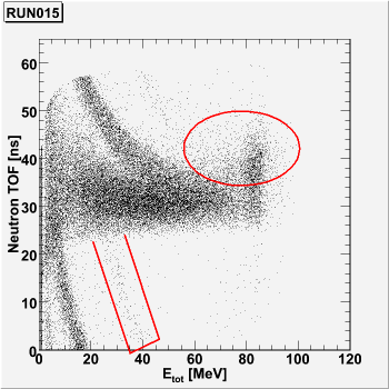
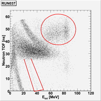
Figure 6.1: TOF shift in T1 in the left panel and run 37 in T8 in the right panel.

One can also note the energy shift in the lower part of the plot, that does not seem to be dependent on the threshold adjustment. If the cause of these problems is because of instabilities in the CFD a possibility to get rid of this problem is to use a timer based on the leading edge technique instead. This will require some extra work with the TOF selections and mean large corrections, since the timing of a leading edge discriminator is dependent on the pulse height.

6.4 Mismatch between T1 and T8

As one can see in figure 6.2 there are some mismatches between T1 and T8. The low energy mismatch has been carefully examined, unfortunately without solving the problem. The intermediate energy mismatch seen in the calcium data in figure 6.2 was however found to depend on the TOF cut. The mismatch was reduced when the upper part of the TOF cut in figure 4.6 was increased. But increasing the TOF cut also increases the amount of accepted low energy neutrons that need to be subtracted from the data. So the chosen TOF cut of two standard deviations from the peak, is a compromise between the error from the telescope matching and the error from the low-energy neutron correction.

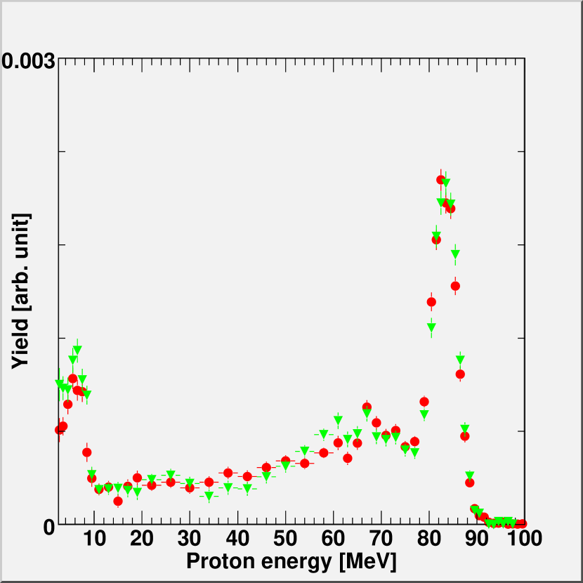
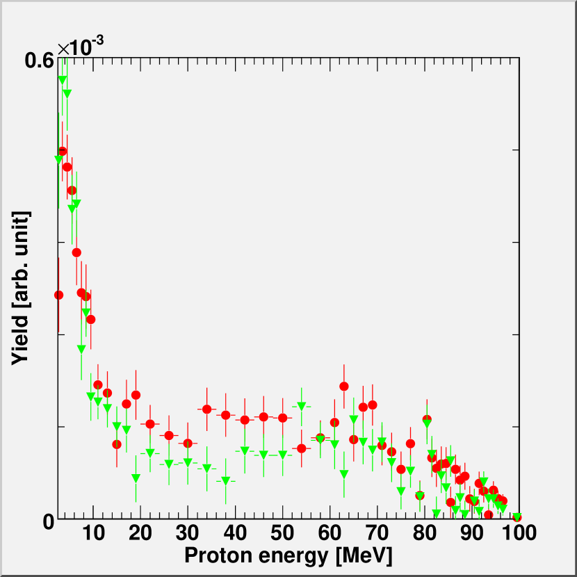
Figure 6.2: Mismatch between T1 (filled circles) and T8 (filled triangles). The left panel shows the CH₂ runs and the right panel shows the calcium runs.

6.5 Reaction losses

Due to nuclear interactions within the CsI(Tl) some protons may, for example, produce gamma radiation that will escape the CsI(Tl) undetected. Thus only a certain fraction of the incident protons is detected at its true energy, and the rest will form a reaction tail of apparently lower energy. This issue is currently under investigation, but so far the results show that for low energies the lost fraction is really small and correcting for these effects only gets important at higher energies, as shown in figure 4.8.

6.6 Different approaches to angular distributions

In this work, the angular distributions were obtained by fitting Eq. (2.11) to the data. This is an approach coming from experiment, and trying to fit some angular shape to the data, that can be integrated to get the cross section. Another approach one can use is to go from theory and calculate the predicted shape, $a$, of the angular distributions and fitting Eq. (2.10) to the data under assumption that $f_{\textrm{MSD}}=1$. The actual form of $f_{\textrm{MSD}}$, as calculated by TALYS, is found in figure 6.5. To calculate $a$, the parametrization used [20] is

$$a=0.04\frac{E_{1}{e_{b}}^{\prime}}{{e_{a}}^{\prime}}+1.8\cdot 10^{-6}\left(\frac{E_{1}{e_{b}}^{\prime}}{{e_{a}}^{\prime}}\right)^{3}+6.7\cdot 10^{-7}\left(\frac{E_{3}{e_{b}}^{\prime}}{{e_{a}}^{\prime}}\right)^{4}$$ (6.1)

where $E_{1}=\min({e_{a}}^{\prime},130)$, $E_{3}=\min({e_{a}}^{\prime},41)$, ${e_{a}}^{\prime}=E_{a}+S_{a}$ and ${e_{b}}^{\prime}=E_{b}+S_{b}$. Here $E_{a}$ is the incoming neutron energy, $E_{b}$ is the outgoing proton energy, and $S_{a,b}$ is the separation energy between particle $a,b$ and the compound nucleus. The separation energy, $S_{a,b}$, is calculated using the Myers and Swiatecki mass formula [14]. As seen in figure 6.5 there exist some differences in angular distributions between the theoretical and the experimental approach, especially at higher energies, where the theory predicts the forward peaking be larger. The negative values on $a$ at really high energies, that would imply backward peaking, are probably statistical artifacts from the background subtraction.

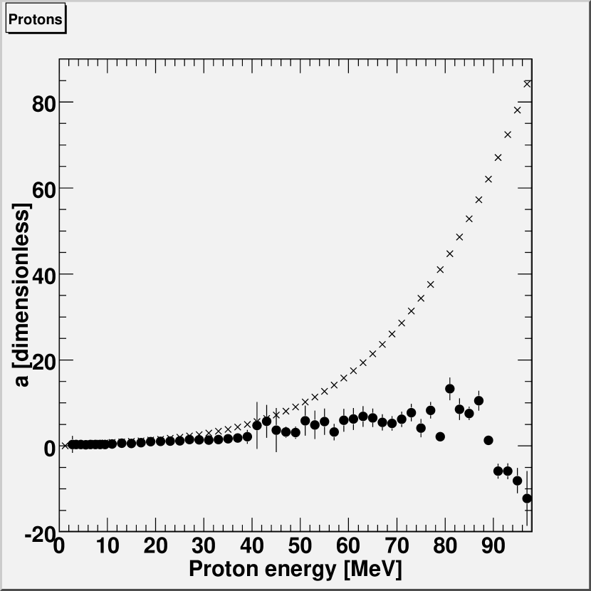
Figure 6.3: Theoretical and experimental values of angular forward peaking, $a$. The values of parameter $a$ are obtained from experimental fits (solid circles) and from Kalbach systematics (crosses).

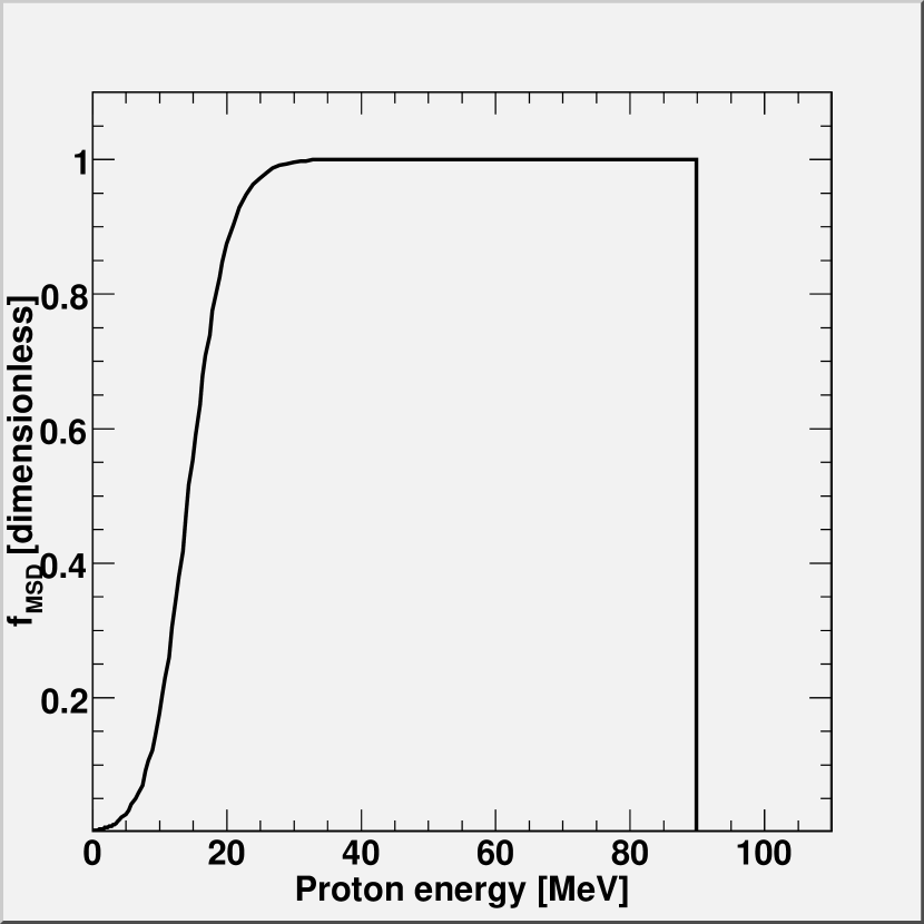
Figure 6.4: Theoretical pre-equilibrium ratio, $f_{\textrm{MSD}}$, as calculated by TALYS.

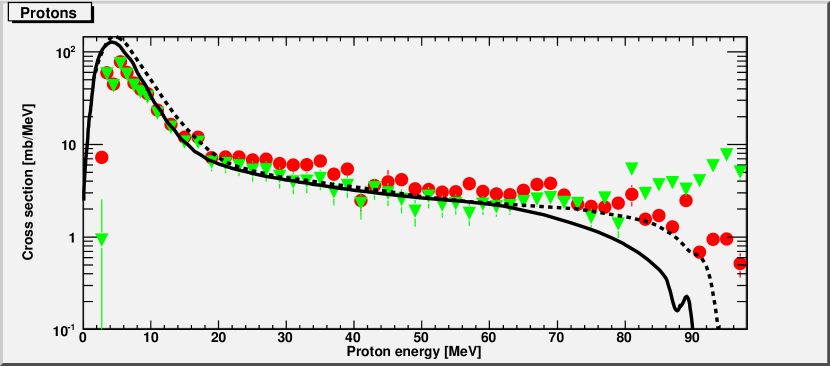
Figure 6.5: Theoretical and experimental approaches to angular distributions and the differences in energy-differential cross sections for the two approaches, where experimental angular distributions are filled circles and calculated angular distribution are filled triangles. The data used are the data with modified TALYS calculations subtracted. The solid line is prediction by TALYS, and the dashed line is prediction by GNASH [40].

As can be seen in figure 6.5, this parametrization gives a result closer to the model at intermediate energies but deviates more at high energies, while at low energies the difference between the methods are small. This is quite expected from the approximation of $f_{\textrm{MSD}}=1$. An investigation of the parametrization with the calculated form of $f_{\textrm{MSD}}$, or even experimental determination of $f_{\textrm{MSD}}$, is something I think could be interesting in the future.

6.7 Systematic uncertainties

Throughout this work the error bars only represent the statistical uncertainties in the experiment. To give a complete picture, the systematic errors should be added to the result. These are listed in table 6.2, where some values are for this particular experiment, and some values are adapted from Tippawan et al. [23].

Origin	Uncertainty
Target correction	1-10 %
Solid angle	1-5 %
Beam monitoring	2-3 %
Number of Ca	1 %
CsI(Tl) efficiency	1 %
Particle identification	1 %
Dead time	$<0.1$ %
Absolute cross section	5 %

Table 6.2: Systematic uncertainties

6.8 Conclusions

As presented in sections 6.1.1-6.1.3 and shown in figures 6.6 - 6.8, comparisons between three different methods have been made. No matter which method one chooses, the results all show the same trend as the previous experiments [22, 23]. The evaporation peak is overestimated by TALYS and predicted to be almost isotropic, while in experiment it significantly decreases with angle. The GNASH calculations overestimate the peak even more. In the pre-equilibrium region, TALYS instead underestimates the cross section, but the predictions seem to be more accurate at larger angles.

The problem in the TOF is an issue that needs to be investigated, especially since similar effects have been noted in other data sets as well [24]. But since one of the mismatches in section 6.4 was found to be dependent on the TOF cut, a solution to the TOF problem might shed some light on the mismatch.

6.9 Outlook

The data sets analyzed in this work was the first, and at this moment the only, data set available from the upgraded neutron facility [26] at TSL. To further improve the calcium results, experimental data from the angles 60, 80, 100 and 120 degrees should be analyzed. The reactions Ca(n,d), Ca(n,t), Ca(n,³He) and Ca(n,$\alpha$) would also be interesting to have a look at.

Apart from that, and as mentioned in section 3, lots of work has previously been carried out at 96 MeV [22, 23, 25] and there still exists a never-ending selection of isotopes to be measured. But since the nuclei under study in these works are especially interesting from a biological and technical point of view it is more interesting to use the capabilities of the new neutron facility and run the experiments at 180 MeV. By obtaining more data sets, one extends the relevant database for future applications. At the same time one makes it possible to do a more quantitative analysis on the nuclei and get a better systematic feedback for the development of TALYS.

Method 1

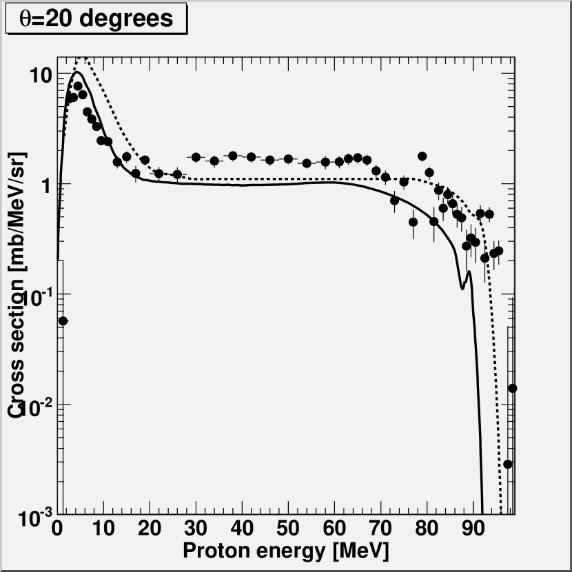
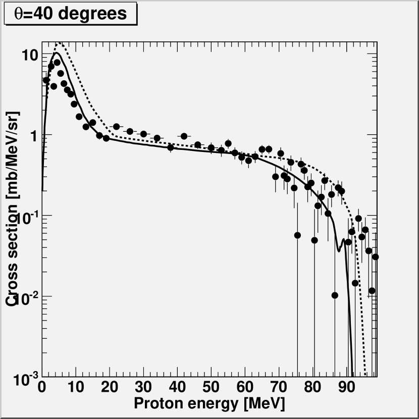
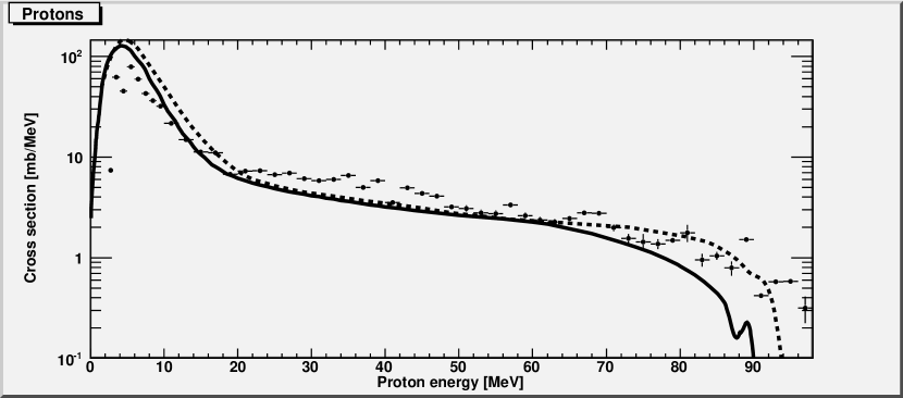
Figure 6.6: Double-differential cross sections in the four top panels, and angle integrated energy-differential cross section in the bottom panel, with experimental data (method 1) subtracted for 94 MeV neutrons in the Ca(n,px) reaction. Solid lines are predictions by TALYS, and dashed lines are predictions by GNASH [40]. Cutoff energy is 2.5 MeV.

Method 2

Method 3

Appendices

Appendix A Figures and tables

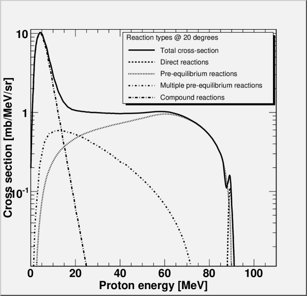
Figure A.1: Contribution to total cross section from various reaction types, according to TALYS calculations.

No	Si1	Si2	Distance [cm]	Angle [deg]	$\Delta x_{1}$ [$\mu$m]	$\Delta x_{2}$ [$\mu$m]
1	38-110B	35-150B	26.83	20	64.9	549
2	37-198D	37-051B	19.83	40	60.5	538
3	38-110D	37-052A	19.83	60	63.9	533
4	37-198G	37-052C	19.83	80	61.7	526
5	31-325C	37-199A	19.83	100	50.4	439
6	31-325D	37-199E	19.83	120	50.1	432
7	38-110G	39-100B	19.83	140	61.6	550
8	31-325H	37-199G	26.83	160	52.9	424

Table A.1: Detector setup

Run	Target	Beam	Neutron fluence	Lifetime	Runtime
		[µA]	[n/cm${{}^{2}}\cdot 10^{8}$]	[%]	[h]
004	Junk
005	Empty	1.2	3.1	84	0:57
006	Empty	1.1	4.2	74	1:15
007	Empty	1.2	5.2	72	1:29
008	Empty		5.5	72	1:35
009	Empty				1:27
010	Empty		5.9	72	1:36
011	Empty	1.2	3.5	72	0:57
012	Empty		5.6	72	1:33
013	Empty		6.9	72	1:55
014	CH2	1.2	6.5	71	1:45
015	CH2		5.5	71	1:33
016	CH2		4.3	71	1:09
017	Empty	1.2	4.7	72	1:22
018	Empty	1.2	4.7	73	1:26
019	Ca	1.1	1.6	74	0:27
020	Ca		5.9	74	1:50
021	Ca		7.1	74	2:02
022	Ca	1.1	7.1	74	2:11
023	Ca		5.9	74	1:47
024	Ca		5.6	74	1:37
025	Ca		4.6	73	1:19
026	CH2		5.1	72	1:28
027	CH2		4.6	72	1:19
028	Ca		7.1	73	2:01
029	Ca		6.9	73	1:56
030	Ca		5.5	73	2:00
031	Ca		3.4	73	0:52
032	Ca		5.7	73	1:37
033	Ca		6.6	73	1:55
034	Ca		7.0	73	2:01
035	Ca		3.7	74	1:06
036	Ca		1.6	74	0:35

Table A.2: List of runs when the table was positioned at 180 degrees, that is with T1 in forward and T8 in backward direction.

Run	Target	Beam	Neutron fluence	Lifetime	Runtime
		[µA]	[n/cm${{}^{2}}\cdot 10^{8}$]	[%]	[h]
001	Junk
002	Junk	1.2
003	Junk	1.2
037	CH2	1.1			1:05
038	Junk
039	CH2	1.1	0.96	71	0:15
040	CH2		5.6	71	1:43
041	CH2	1.1	5.5	71	1:35
042	CH2		1.8	71	0:30
043	CH2		6.9	71	2:00
044	Empty		5.9	72	1:44
045	Empty		9.3	72	2:44
046	Empty		7.2	72	2:07
047	Empty		6.9	72	2:00
048	Empty		7.0	72	2:01
049	Empty		6.7	72	1:59
050	Empty		6.8	72	2:00
051	Empty		5.2	72	1:31
052	Ca	1.1	4.5	71	1:15
053	Ca	1.1	5.3	72	1:37
054	Ca	1.1	5.4	72	1:35
055	Ca		5.7	72	1:45
056	Ca		3.4	72	1:00
057	Ca		4.7	72	1:25
058	Ca		6.4	71	1:55
059	Ca		6.9	71	2:02
060	Ca		6.4	71	1:56
061	Ca		6.6	71	2:01
062	Ca		4.2	72	1:17
063	Ca	1.1	5.4	72	1:39
064	Ca	1.1	6.5	72	1:59
065	Ca		6.5	72	1:59
066	Ca		3.5	72	1:02

Table A.3: List of runs when the table was positioned at 0 degrees, that is with T8 in forward and T1 in backward direction.

013C	4264	04FE	0000	0000	4265	05B2	0000	0000	4266
083E	0000	0000	4267	039B	0000	0000	4268	06B5	0000
0000	4269	06F4	0000	0000	426A	048B	0000	0000	426B
0325	0000	0000	426C	0A2C	0000	0000	426D	074E	0000
0000	426E	0C53	0000	0000	426F	000E	0000	0000	4270
02D9	0000	0000	4271	0000	0000	0000	4272	0000	0000
0000	4273	0000	0000	0000	4274	0000	0000	0000	4275
0000	0000	0000	4276	0000	0000	0000	4277	0000	0000
0000	4501	0066	0065	004F	0000	01F4	4502	004B	02CA
0137	0000	007E	4503	007A	0068	0040	0000	001C	4504
004B	0034	0043	0000	0206	4505	0064	005A	0036	0000
01F5	4506	0077	0049	003F	0000	01CF	4507	0062	006D
00D4	0000	0225	4508	0083	0065	004D	0000	01D3	480A
0060	0068	0067	004D	0069	0047	005A	0062	0000	4C09
0025	0038	004A	004E	0040	0039	002E	002F	0FDC	0FDC
0FDC	0FDC	0000	4300	0000	0083	018F	FFFF

Figure A.2: Typical sequence of hexadecimal raw data for an event. Group identifiers are marked in bold. Groups 42XX are the scalers, 45XX are the readout from the telescopes and the group 4300 0000 is the identifier for the RF signals. The event is ended by FFFF.

	T1	T2	T7	T8
$k_{1}$	0.00334	0.00332	0.00309	0.00278
$m_{1}$	-0.264	-0.197	-0.284	-0.256
$k_{2}$	0.00893	0.00863	0.00969	0.00904
$m_{2}$	-0.851	-0.667	-1.04	-0.893
$a$	-2.09	-0.734	-1.57	-1.49
$b$	0.0259	0.0199	0.0226	0.0228
$c$	0.0032	0.0032	0.0032	0.0032

Table A.4: Calibration values, as used in Eq. (4.1) and Eq. (4.3).

Neutron bin [MeV]	np bin [MeV]	$\sigma_{(\textrm{n},\textrm{p})}$ [mb]
5-15	4-13	292.60
15-25	13-22	153.78
25-35	22-31	100.51
35-45	31-40	73.033
45-55	40-48	57.336
55-65	48-57	47.461
65-75	57-66	40.841
75-85	66-78	36.239

Table A.5: Energy binning for subtraction of carbon data from the CH₂ runs.

Bin	Uncorrected	Corrected	Bin	Uncorrected	Corrected
[MeV]	[mb/sr/MeV]		[MeV]	[mb/sr/MeV]
2.5-3	$0.0931\pm 0.23$	$0.0559\pm 0.25$	68-70	$2.67\pm 0.30$	$2.25\pm 0.37$
3-4	$9.61\pm 0.75$	$5.66\pm 1.1$	70-72	$2.13\pm 0.29$	$1.85\pm 0.32$
4-5	$9.81\pm 0.50$	$5.90\pm 0.86$	72-74	$1.87\pm 0.28$	$1.67\pm 0.30$
5-6	$12.5\pm 0.50$	$7.71\pm 1.00$	74-76	$1.15\pm 0.26$	$1.07\pm 0.26$
6-7	$10.4\pm 0.50$	$6.54\pm 0.95$	76-78	$1.69\pm 0.25$	$1.59\pm 0.25$
7-8	$7.29\pm 0.45$	$4.79\pm 0.75$	78-80	$0.73\pm 0.22$	$0.716\pm 0.22$
8-9	$6.25\pm 0.44$	$4.13\pm 0.73$	80-81	$2.89\pm 0.30$	$2.88\pm 0.30$
9-10	$5.37\pm 0.40$	$3.61\pm 0.68$	81-82	$2.05\pm 0.28$	$2.05\pm 0.28$
10-12	$4.00\pm 0.28$	$2.68\pm 0.45$	82-83	$0.739\pm 0.26$	$0.739\pm 0.26$
12-14	$3.93\pm 0.30$	$2.60\pm 0.53$	83-84	$1.42\pm 0.26$	$1.42\pm 0.26$
14-16	$2.56\pm 0.31$	$1.66\pm 0.45$	84-85	$0.979\pm 0.23$	$0.979\pm 0.23$
16-18	$2.86\pm 0.35$	$1.83\pm 0.53$	85-86	$1.3\pm 0.23$	$1.30\pm 0.23$
18-20	$2.02\pm 0.35$	$1.28\pm 0.47$	86-87	$1.07\pm 0.21$	$1.07\pm 0.21$
20-24	$2.66\pm 0.28$	$1.68\pm 0.41$	87-88	$0.861\pm 0.21$	$0.861\pm 0.21$
24-28	$2.00\pm 0.30$	$1.25\pm 0.39$	88-89	$0.801\pm 0.20$	$0.801\pm 0.20$
28-32	$1.98\pm 0.31$	$1.23\pm 0.39$	89-90	$0.444\pm 0.18$	$0.444\pm 0.18$
32-36	$2.83\pm 0.33$	$1.74\pm 0.46$	90-91	$0.524\pm 0.17$	$0.524\pm 0.17$
36-40	$2.61\pm 0.33$	$1.59\pm 0.46$	91-92	$0.479\pm 0.17$	$0.479\pm 0.17$
40-44	$2.92\pm 0.32$	$1.78\pm 0.49$	92-93	$0.874\pm 0.17$	$0.874\pm 0.17$
44-48	$2.85\pm 0.31$	$1.75\pm 0.47$	93-94	$0.345\pm 0.14$	$0.345\pm 0.14$
48-52	$2.66\pm 0.29$	$1.69\pm 0.43$	94-95	$0.862\pm 0.13$	$0.862\pm 0.13$
52-56	$2.72\pm 0.28$	$1.83\pm 0.40$	95-96	$0.380\pm 0.11$	$0.380\pm 0.11$
56-60	$2.49\pm 0.26$	$1.77\pm 0.35$	96-97	$0.400\pm 0.10$	$0.400\pm 0.10$
60-62	$2.56\pm 0.35$	$1.92\pm 0.45$	97-98	$-0.0245\pm 0.080$	$-0.0245\pm 0.080$
62-64	$2.57\pm 0.33$	$1.99\pm 0.43$	98-99	$0.00468\pm 0.079$	$0.00468\pm 0.079$
64-66	$2.73\pm 0.32$	$2.18\pm 0.41$	99-100	$0.0227\pm 0.13$	$0.0227\pm 0.13$
66-68	$2.80\pm 0.316$	$2.27\pm 0.41$

Table A.6: Experimental double-differential cross sections at 20 degrees in the Ca(n,px) reaction for the neutron spectrum in table 4.3 and for 94 MeV neutrons according to the subtraction method in section 6.1.3.

Bin	Uncorrected	Corrected	Bin	Uncorrected	Corrected
[MeV]	[mb/sr/MeV]		[MeV]	[mb/sr/MeV]
2.5-3	$7.64\pm 1.9$	$4.59\pm 2.2$	70-71	$0.489\pm 0.17$	$0.428\pm 0.19$
3-4	$11.3\pm 0.57$	$6.68\pm 1.0$	71-72	$0.950\pm 0.18$	$0.834\pm 0.22$
4-5	$6.43\pm 0.24$	$3.87\pm 0.51$	72-73	$0.506\pm 0.17$	$0.456\pm 0.18$
5-6	$12.6\pm 0.34$	$7.80\pm 0.95$	73-74	$0.459\pm 0.16$	$0.414\pm 0.17$
6-7	$9.31\pm 0.30$	$5.84\pm 0.78$	74-75	$0.738\pm 0.16$	$0.689\pm 0.17$
7-8	$6.97\pm 0.28$	$4.59\pm 0.63$	75-76	$0.355\pm 0.15$	$0.334\pm 0.16$
8-9	$5.80\pm 0.27$	$3.84\pm 0.60$	76-77	$0.0924\pm 0.14$	$0.0861\pm 0.14$
9-10	$5.16\pm 0.25$	$3.47\pm 0.58$	77-78	$0.700\pm 0.15$	$0.667\pm 0.15$
10-12	$3.87\pm 0.16$	$2.60\pm 0.38$	78-79	$0.586\pm 0.14$	$0.571\pm 0.14$
12-14	$2.72\pm 0.15$	$1.81\pm 0.34$	79-80	$0.366\pm 0.13$	$0.362\pm 0.13$
14-16	$2.03\pm 0.16$	$1.33\pm 0.31$	80-81	$0.411\pm 0.13$	$0.409\pm 0.13$
16-18	$2.29\pm 0.17$	$1.48\pm 0.37$	81-82	$0.0804\pm 0.11$	$0.0804\pm 0.11$
18-20	$1.58\pm 0.18$	$1.01\pm 0.31$	82-83	$0.215\pm 0.12$	$0.215\pm 0.12$
20-24	$1.47\pm 0.14$	$0.926\pm 0.22$	83-84	$0.274\pm 0.11$	$0.274\pm 0.11$
24-28	$2.04\pm 0.15$	$1.28\pm 0.29$	84-85	$0.439\pm 0.10$	$0.439\pm 0.10$
28-32	$1.78\pm 0.15$	$1.11\pm 0.27$	85-86	$0.172\pm 0.094$	$0.172\pm 0.094$
32-36	$1.65\pm 0.15$	$1.02\pm 0.27$	86-87	$0.295\pm 0.089$	$0.295\pm 0.089$
36-40	$1.48\pm 0.15$	$0.907\pm 0.25$	87-88	$0.0167\pm 0.076$	$0.0167\pm 0.076$
40-44	$1.13\pm 0.15$	$0.694\pm 0.22$	88-89	$0.360\pm 0.080$	$0.36\pm 0.080$
44-48	$1.55\pm 0.14$	$0.971\pm 0.26$	89-90	$0.325\pm 0.10$	$0.325\pm 0.10$
48-52	$1.22\pm 0.13$	$0.785\pm 0.21$	90-91	$-0.202\pm 0.00$	$-0.202\pm 0.00$
52-54	$1.12\pm 0.18$	$0.746\pm 0.27$	91-92	$0.076\pm 0.074$	$0.076\pm 0.074$
54-56	$1.04\pm 0.18$	$0.720\pm 0.25$	92-93	$0.102\pm 0.047$	$0.102\pm 0.047$
56-58	$1.26\pm 0.17$	$0.897\pm 0.27$	93-94	$0.0237\pm 0.063$	$0.0237\pm 0.063$
58-60	$0.966\pm 0.16$	$0.712\pm 0.23$	94-95	$0.149\pm 0.046$	$0.149\pm 0.046$
60-62	$0.851\pm 0.16$	$0.647\pm 0.2$	95-96	$0.0882\pm 0.046$	$0.0882\pm 0.046$
62-64	$0.773\pm 0.15$	$0.605\pm 0.18$	96-97	$0.108\pm 0.046$	$0.108\pm 0.046$
64-66	$0.871\pm 0.14$	$0.701\pm 0.19$	97-98	$0.0595\pm 0.044$	$0.0595\pm 0.044$
66-68	$1.07\pm 0.14$	$0.876\pm 0.19$	98-99	$0.0190\pm 0.045$	$0.0190\pm 0.045$
68-70	$1.07\pm 0.13$	$0.909\pm 0.18$	99-100	$0.0499\pm 0.050$	$0.0499\pm 0.050$

Table A.7: Experimental double-differential cross sections at 40 degrees in the Ca(n,px) reaction for the neutron spectrum in table 4.3 and for 94 MeV neutrons according to the subtraction method in section 6.1.3.

Bin	Uncorrected	Corrected	Bin	Uncorrected	Corrected
[MeV]	[mb/sr/MeV]		[MeV]	[mb/sr/MeV]
2.5-3	$0.0668\pm 0.14$	$0.0401\pm 0.15$	30-35	$0.175\pm 0.020$	$0.114\pm 0.082$
3-4	$5.41\pm 0.42$	$3.19\pm 0.60$	35-40	$0.0721\pm 0.015$	$0.0472\pm 0.045$
4-5	$3.90\pm 0.20$	$2.35\pm 0.35$	40-45	$0.0183\pm 0.011$	$0.0123\pm 0.018$
5-6	$8.68\pm 0.30$	$5.37\pm 0.69$	45-50	$0.00676\pm 0.0082$	$0.00474\pm 0.010$
6-7	$6.76\pm 0.27$	$4.26\pm 0.59$	50-55	$-0.0278\pm 0.0090$	$-0.0208\pm 0.031$
7-8	$4.21\pm 0.21$	$2.80\pm 0.41$	55-60	$0.0146\pm 0.0085$	$0.0117\pm 0.020$
8-9	$3.55\pm 0.18$	$2.37\pm 0.39$	60-65	$0.0244\pm 0.0099$	$0.0209\pm 0.033$
9-10	$3.37\pm 0.16$	$2.31\pm 0.39$	65-70	$0.0274\pm 0.0090$	$0.0246\pm 0.041$
10-12	$1.97\pm 0.055$	$1.36\pm 0.20$	70-75	$0.00282\pm 0.011$	$0.00267\pm 0.011$
12-14	$1.09\pm 0.045$	$0.762\pm 0.15$	75-80	$0.0165\pm 0.011$	$0.0161\pm 0.021$
14-16	$0.946\pm 0.046$	$0.663\pm 0.16$	80-85	$0.0562\pm 0.013$	$0.0561\pm 0.014$
16-18	$0.709\pm 0.052$	$0.493\pm 0.16$	85-90	$0.0346\pm 0.015$	$0.0346\pm 0.015$
18-20	$0.283\pm 0.053$	$0.193\pm 0.096$	90-95	$0.0914\pm 0.016$	$0.0914\pm 0.016$
20-25	$0.420\pm 0.024$	$0.280\pm 0.11$	95-100	$0.0274\pm 0.019$	$0.0274\pm 0.019$
25-30	$0.149\pm 0.0233$	$0.0968\pm 0.057$

Table A.8: Experimental double-differential cross sections at 140 degrees in the Ca(n,px) reaction for the neutron spectrum in table 4.3 and for 94 MeV neutrons according to the subtraction method in section 6.1.3.

Bin	Uncorrected	Corrected	Bin	Un-corrected	Corrected
[MeV]	[mb/sr/MeV]		[MeV]	[mb/sr/MeV]
2.5-3	$0.152\pm 0.26$	$0.0915\pm 0.28$	30-35	$0.152\pm 0.023$	$0.0984\pm 0.073$
3-4	$6.70\pm 0.60$	$3.95\pm 0.81$	35-40	$0.204\pm 0.020$	$0.133\pm 0.12$
4-5	$6.44\pm 0.38$	$3.87\pm 0.61$	40-45	$0.137\pm 0.017$	$0.0918\pm 0.10$
5-6	$6.97\pm 0.36$	$4.31\pm 0.62$	45-50	$0.0132\pm 0.015$	$0.00927\pm 0.019$
6-7	$4.68\pm 0.32$	$2.95\pm 0.50$	50-55	$0.0163\pm 0.015$	$0.0122\pm 0.023$
7-8	$4.05\pm 0.30$	$2.69\pm 0.46$	55-60	$-0.00418\pm 0.017$	$-0.00335\pm 0.018$
8-9	$3.63\pm 0.25$	$2.43\pm 0.44$	60-65	$-0.00651\pm 0.019$	$-0.00558\pm 0.021$
9-10	$2.89\pm 0.21$	$1.98\pm 0.38$	65-70	$-0.0545\pm 0.019$	$-0.0491\pm 0.081$
10-12	$1.59\pm 0.083$	$1.10\pm 0.17$	70-75	$0.0539\pm 0.021$	$0.0511\pm 0.073$
12-14	$0.915\pm 0.079$	$0.640\pm 0.14$	75-80	$0.0449\pm 0.024$	$0.0439\pm 0.055$
14-16	$0.647\pm 0.079$	$0.454\pm 0.14$	80-85	$0.134\pm 0.023$	$0.134\pm 0.026$
16-18	$0.616\pm 0.080$	$0.428\pm 0.16$	85-90	$0.146\pm 0.028$	$0.146\pm 0.028$
18-20	$0.388\pm 0.078$	$0.266\pm 0.13$	90-95	$0.254\pm 0.030$	$0.254\pm 0.030$
20-25	$0.223\pm 0.030$	$0.148\pm 0.063$	95-100	$0.229\pm 0.036$	$0.229\pm 0.036$
25-30	$0.184\pm 0.0281$	$0.120\pm 0.070$

Table A.9: Experimental double-differential cross sections at 160 degrees in the Ca(n,px) reaction for the neutron spectrum in table 4.3 and for 94 MeV neutrons according to the subtraction method in section 6.1.3.

Bin	Uncorrected	Corrected	Bin	Uncorrected	Corrected
[MeV]	[mb/MeV]		[MeV]	[mb/MeV]
0-2.5	-	-	46-48	$6.69\pm 0.29$	$4.15\pm 0.41$
2.5-3	$12.1\pm 0.32$	$7.24\pm 0.36$	48-50	$5.23\pm 0.28$	$3.32\pm 0.37$
3-4	$102\pm 0.52$	$59.7\pm 0.77$	50-52	$5.04\pm 0.35$	$3.26\pm 0.55$
4-5	$73.7\pm 0.26$	$45.0\pm 0.47$	52-54	$4.54\pm 0.33$	$3.05\pm 0.56$
5-6	$129\pm 0.33$	$78.7\pm 0.73$	54-56	$4.46\pm 0.33$	$3.07\pm 0.49$
6-7	$97.3\pm 0.30$	$60.4\pm 0.62$	56-58	$5.44\pm 0.29$	$3.77\pm 0.53$
7-8	$69.7\pm 0.26$	$46.1\pm 0.49$	58-60	$4.27\pm 0.32$	$3.12\pm 0.44$
8-9	$59.2\pm 0.24$	$39.5\pm 0.47$	60-62	$3.85\pm 0.31$	$2.91\pm 0.39$
9-10	$52.5\pm 0.21$	$35.4\pm 0.45$	62-64	$3.68\pm 0.30$	$2.86\pm 0.37$
10-12	$35.2\pm 0.11$	$23.6\pm 0.26$	64-66	$4.00\pm 0.27$	$3.21\pm 0.36$
12-14	$24.2\pm 0.10$	$16.4\pm 0.23$	66-68	$4.54\pm 0.29$	$3.70\pm 0.37$
14-16	$18.3\pm 0.10$	$12.0\pm 0.22$	68-70	$4.50\pm 0.28$	$3.79\pm 0.35$
16-18	$18.0\pm 0.11$	$12.0\pm 0.26$	70-72	$3.25\pm 0.24$	$2.84\pm 0.28$
18-20	$11.0\pm 0.13$	$7.19\pm 0.22$	72-74	$2.53\pm 0.27$	$2.27\pm 0.28$
20-22	$11.8\pm 0.11$	$7.34\pm 0.24$	74-76	$2.34\pm 0.45$	$2.15\pm 0.32$
22-24	$12.0\pm 0.11$	$7.35\pm 0.27$	76-78	$2.23\pm 0.25$	$2.11\pm 0.25$
24-26	$10.9\pm 0.12$	$6.82\pm 0.28$	78-80	$2.42\pm 0.12$	$2.33\pm 0.20$
26-28	$11.3\pm 0.14$	$6.95\pm 0.30$	80-82	$2.89\pm 0.56$	$2.89\pm 0.74$
28-30	$10.0\pm 0.14$	$6.25\pm 0.31$	82-84	$1.55\pm 0.23$	$1.55\pm 0.19$
30-32	$9.53\pm 0.12$	$5.99\pm 0.31$	84-86	$1.71\pm 0.15$	$1.71\pm 0.15$
32-34	$9.74\pm 0.12$	$6.04\pm 0.39$	86-88	$1.29\pm 0.21$	$1.29\pm 0.21$
34-36	$10.7\pm 0.13$	$6.64\pm 0.46$	88-90	$2.47\pm 0.070$	$2.47\pm 0.070$
36-38	$8.17\pm 0.11$	$4.76\pm 0.39$	90-92	$0.684\pm 0.045$	$0.684\pm 0.041$
38-40	$9.51\pm 0.12$	$5.42\pm 0.61$	92-94	$0.942\pm 0.044$	$0.942\pm 0.044$
40-42	$5.76\pm 0.13$	$2.49\pm 0.77$	94-96	$0.949\pm 0.060$	$0.949\pm 0.060$
42-44	$8.05\pm 0.21$	$3.59\pm 0.68$	96-98	$0.516\pm 0.15$	$0.516\pm 0.15$
44-46	$7.12\pm 0.32$	$3.94\pm 1.3$	98-100	$0.315\pm 0.15$	$0.315\pm 0.15$
44-46	$7.12\pm 0.31$	$3.94\pm 0.41$

Table A.10: Experimental energy-differential cross sections in the Ca(n,px) reaction for the neutron spectrum in table 4.3 and for 94 MeV neutrons according to the subtraction method in section 6.1.3.

Angle	Uncorrected	Corrected
[deg]	[mb/sr]
20	$253\pm 4.76$	$175\pm 6.69$
40	$162\pm 2.51$	$107\pm 4.22$
140	$51.5\pm 0.792$	$33.7\pm 1.73$
160	$52.4\pm 1.14$	$35.1\pm 2.04$

Table A.11: Experimental angular-differential cross sections in the Ca(n,px) reaction for the neutron spectrum in table 4.3 and for 94 MeV neutrons according to the subtraction method in section 6.1.3. Cutoff energy is 2.5 MeV.

Uncorrected	Corrected
[mb]
$1220\pm 3.21$	$788\pm 5.83$

Table A.12: Experimental total cross sections in the Ca(n,px) reaction for the neutron spectrum in table 4.3 and for 94 MeV neutrons according to the subtraction method in section 6.1.3. Cutoff energy is 2.5 MeV.

Appendix B Notes about extracting information from NN databases

When using databases to obtain data on elastic Nucleon-Nucleon (NN) scattering it is not always intuitive to get what one wants from it. The problem is that NN databases often gives the cross section for a given neutron scattering angle, but one most often knows the proton angle. To get the cross section one wants, some transformations between different frames and calculations of ratio-factors are needed [42]. This is an eight-step process to get through this without (too many) tears. First some necessary kinematic relations for a general scattering reaction are given in [18],

$$E_{1}=T_{1}+m_{1}$$ (B.1a)

$$p_{1}=\sqrt{T_{1}^{2}+2T_{1}m_{1}}$$ (B.1b)

$$s=m_{1}^{2}+m_{2}^{2}+2E_{1}m_{2}$$ (B.1c)

$$E_{3}^{\textrm{cm}}=\frac{1}{2\sqrt{s}}\left(s+m_{3}^{2}-m_{4}^{2}\right)$$ (B.1d)

$$v_{\textrm{cm}}=\frac{p_{1}}{E_{1}+m_{2}}$$ (B.1e)

$$p_{3}^{\textrm{cm}}=\sqrt{(E_{3}^{\textrm{cm}})^{2}-m_{3}^{2}}$$ (B.1f)

$$\tan\theta_{3}=\frac{\sin\theta_{3}^{\textrm{cm}}\sqrt{1-v_{\textrm{cm}}^{2}}}{\cos\theta_{3}^{\textrm{cm}}+\frac{v_{\textrm{cm}}E_{3}^{\textrm{cm}}}{p_{3}^{\textrm{cm}}}}.$$ (B.1g)

The relevant quantities are defined in figure B.3, where $m_{i}$ is the mass, $T_{i}$ is the kinetic energy and $p_{i}$ is the momentum of particle $i$. Quantities in the CM system are labeled cm, unlabeled quantities are in the laboratory frame.

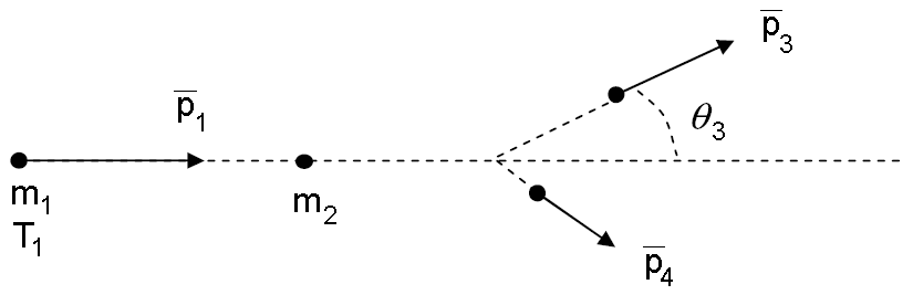
Figure B.3: Scattering in the laboratory frame, adapted from [18].

For a NN reaction with a neutron on a proton target we switch the indices in the notations as $1,4\rightarrow n$ and $2,3\rightarrow p$. Known parameters are assumed to be $m_{p}$, $m_{n}$, $T_{n}$ and $\theta_{\textrm{lab}}^{p}$. An unlabeled $\theta$ is always the scattering angle of the neutron.

1. Using the relations (B.1a) to (B.1g) it is straightforward, although (B.1g) might make it analytically tricky, to calculate $\theta^{\textrm{cm}}_{p}$.

2. The easy part: $\theta^{\textrm{cm}}_{n}=180-\theta^{\textrm{cm}}_{p}$.

3. Calculate $\theta^{\textrm{lab}}_{n}$. This is preferably done via some computer code for relativistic kinematics, for example the code RELKIN circulating at Department of Neutron Physics, Uppsala University (INF) [30].

4. From the NN database of choice, extract the cross section in the CM frame for the opposite case, that is when the neutron is scattered in the desired proton angle. That is, the cross section $\left(\frac{\textrm{d}\sigma}{\textrm{d}\Omega}\right)^{\textrm{cm}}_{\theta_{n}=\theta^{\textrm{cm}}_{p}}$.

5. In the same way as in step 4, use a NN database to extract the cross section in the CM frame for the desired case. That is, the cross section $\left(\frac{\textrm{d}\sigma}{\textrm{d}\Omega}\right)^{\textrm{cm}}_{\theta_{n}=\theta^{\textrm{cm}}_{n}}$.

6. Do step 4, but in the laboratory frame, to get $\left(\frac{\textrm{d}\sigma}{\textrm{d}\Omega}\right)^{\textrm{lab}}_{\theta_{n}=\theta^{\textrm{lab}}_{p}}$ from the NN database.

7. Now to calculate the ratio factor, $R$, introduced in [42] for transformations between lab frame cross section and CM frame cross section. Since the $R$ given in the reference only is valid for particles of equal masses the results from step 4 and step 6 is used to calculate $R$ explicitly from the relation $\left(\frac{\textrm{d}\sigma}{\textrm{d}\Omega}\right)^{\textrm{cm}}_{\theta_{n}=\theta^{\textrm{cm}}_{p}}=R\left(\frac{\textrm{d}\sigma}{\textrm{d}\Omega}\right)^{\textrm{lab}}_{\theta_{n}=\theta^{\textrm{lab}}_{p}}$.

8. Using $R$ obtained in step 7 it is now possible to transform the cross section from step 5 into the lab frame, by the relation previously used and obtained from [42], $\left(\frac{\textrm{d}\sigma}{\textrm{d}\Omega}\right)^{\textrm{lab}}_{\theta_{n}=\theta^{\textrm{lab}}_{n}}=\left(\frac{\textrm{d}\sigma}{\textrm{d}\Omega}\right)^{\textrm{cm}}_{\theta_{n}=\theta^{\textrm{cm}}_{n}}\frac{1}{R}$.

Finally we have the cross section $\left(\frac{\textrm{d}\sigma}{\textrm{d}\Omega}\right)^{\textrm{lab}}_{\theta=\theta^{\textrm{lab}}_{n}}$ which is just what we wanted, since the cross section of scattering a neutron at an angle of $\theta^{\textrm{lab}}_{n}$ is equivalent to the cross section of scattering of a proton at an angle $\theta^{\textrm{lab}}_{p}$.

 

• Let us find the cross section for np scattering at $\theta_{\textrm{lab}}^{p}=20$ degrees with an incoming neutron energy of $T_{n}=50$ MeV. Using the mass values $m_{n}=939.57$ MeV/c² and $m_{n}=938.27$ MeV/c² the relations (B.1a) to (B.1g) will give $\theta^{\textrm{cm}}_{p}\approx 40.5$ degrees and, consequentially, $\theta^{\textrm{cm}}_{n}\approx 139.5$ degrees. Using RELKIN [30], a code for relativistic kinematics, $\theta^{\textrm{lab}}_{p}$ is calculated to be $\theta^{\textrm{lab}}_{p}\approx 69.4$ degrees. From the SAID NN database [41] we get

  $$\left(\frac{\textrm{d}\sigma}{\textrm{d}\Omega}\right)^{\textrm{cm}}_{\theta_{n}=40.5}\approx 14.1\frac{\textrm{mb}}{\textrm{sr}}$$ (B.2a)

  $$\left(\frac{\textrm{d}\sigma}{\textrm{d}\Omega}\right)^{\textrm{cm}}_{\theta_{n}=139.5}\approx 15.0\frac{\textrm{mb}}{\textrm{sr}}$$ (B.2b)

  $$\left(\frac{\textrm{d}\sigma}{\textrm{d}\Omega}\right)^{\textrm{lab}}_{\theta_{n}=20.0}\approx 53.9.\frac{\textrm{mb}}{\textrm{sr}}$$ (B.2c)

  Note the different observable keywords DSG for cross section in the center of mass frame, and DSGL for the cross section in the laboratory frame. The ratio factor, $R$, can now be calculated using the information in (B.2a), (B.2c) and the definition in step 7

  $$R\equiv\frac{\left(\frac{\textrm{d}\sigma}{\textrm{d}\Omega}\right)^{\textrm{cm}}_{\theta_{n}=\theta^{\textrm{cm}}_{p}}}{\left(\frac{\textrm{d}\sigma}{\textrm{d}\Omega}\right)^{\textrm{lab}}_{\theta_{n}=\theta^{\textrm{lab}}_{p}}}=\frac{14.1}{53.9}\approx 0.261.$$ (B.3)

  The ratio factor from (B.3) and the cross section (B.2b) can now be used to obtain

  $$\left(\frac{\textrm{d}\sigma}{\textrm{d}\Omega}\right)^{\textrm{lab}}_{\theta_{n}=69.4}=\left(\frac{\textrm{d}\sigma}{\textrm{d}\Omega}\right)^{\textrm{cm}}_{\theta_{n}=139.5}\frac{1}{R}=15.0\cdot\frac{1}{0.261}\approx 57.5\frac{\textrm{mb}}{\textrm{sr}}$$ (B.4)

  which is the sought cross section.

References

- Chadwick [1932] J. Chadwick. The Existence of a Neutron. Proceedings of the Royal Society of London. Series A, Containing Papers of a Mathematical and Physical Character, 136(830):692–708, June 1932.
- Bothe and Becker [1930] W. Bothe and H. Becker. Künstliche Erregung von Kern--Strahlen. Zeitschrift fur Physik, 66:289–306, December 1930.
- Nordling and Österman [1999] C. Nordling and J. Österman. Physics Handbook for Science and Engineering. Studentlitteratur, 6th edition, 1999.
- Baker et al. [2006] C. A. Baker, D. D. Doyle, P. Geltenbort, K. Green, M. G. D. van der Grinten, P. G. Harris, P. Iaydjiev, S. N. Ivanov, D. J. R. May, J. M. Pendlebury, J. D. Richardson, D. Shiers, and K. F. Smith. Improved Experimental Limit on the Electric Dipole Moment of the Neutron. Physical Review Letters, 97(131801), September 2006.
- Adler et al. [1974] M. J. Adler, W. Benton, and C. E. Swanson, editors. The new Encyclopædia Britannica, volume II of Micropædia. Encyclopædia Britannica, inc., Chicago, 15th edition, 1974.
- Campbell and Reece [2001] N. Campbell and J. Reece. Biology. Benjamin Cummings, San Francisco, 6th edition, December 2001.
- Baker and Holloway [1944] C. P. Baker and M. G. Holloway. Note on the origin of the term “barn”. Technical Report LAMS-523, Los Alamos National Laboratory, Los Alamos, USA, September 1944.
- McCann and Graff [2001] J. L. McCann and R. L. Graff. Radioactive Man in Planet of the Strange-O’s. In M. Groening, editor, Simpsons Comics Royale. Harper Paperbacks, 2001.
- Nias [1998] A. H. W. Nias. An Introduction to Radiobiology. John Wiley & Sons, West Sussex, England, 2nd edition, July 1998.
- [10] H. Lundqvist. Material from the course 1TT746 Medical techniques and radiobiology, Uppsala University.
- Petti and Lennox [1994] P. L. Petti and A. J. Lennox. Hadronic Radiotherapy. Annual Review of Nuclear and Particle Science, 44:155–197, December 1994.
- Tippawan [2004] U. Tippawan. Secondary particle spectra from neutron induced nuclear reaction in the 14-100 MeV region. PhD thesis, Chiang Mai University, Chiang Mai, Thailand, May 2004.
- Koning et al. [2005] A. J. Koning, S. Hilaire, and M. C. Duijvestijn. TALYS: Comprehensive Nuclear Reaction Modeling. In R. C. Haight, P. Talou, T. Kawano, and M. B. Chadwick, editors, AIP Conference Proceedings 769: International Conference on Nuclear Data for Science and Technology, pages 1154–1159, May 2005.
- Koning et al. [2004] A. J. Koning, S. Hilaire, and M. C. Duijvestijn. Talys-0.64 User Manual. NRG Report 21297/04.62741/P FAI/AK/AK, December 2004.
- Krane [1987] K. S. Krane. Introductory Nuclear Physics. John Wiley & Sons, Inc., 2nd edition, 1987.
- Herzberg et al. [2006] R.-D. Herzberg, P. T. Greenlees, P. A. Butler, G. D. Jones, M. Venhart, I. G. Darby, S. Eeckhaudt, K. Eskola, T. Grahn, C. Gray-Jones, F. P. Hessberger, P. Jones, R. Julin, S. Juutinen, S. Ketelhut, W. Korten, M. Leino, A.-P. Leppänen, S. Moon, M. Nyman, R. D. Page, J. Pakarinen, A. Pritchard, P. Rahkila, J. Sarén, C. Scholey, A. Steer, Y. Sun, Ch. Theisen, and J. Uusitalo. Nuclear isomers in superheavy elements as stepping stones towards the island of stability. Nature, 442:896–899, August 2006.
- Koning and Delaroche [2003] A. J. Koning and J. P. Delaroche. Local and global nucleon optical models from 1 keV to 200 MeV. Nuclear Physics A, 713:231–310, January 2003.
- Höistad [2005] B. Höistad. Lecture Notes in Nuclear Physics, 2005.
- Koning and Duijvestijn [2004] A. J. Koning and M. C. Duijvestijn. A global pre-equilibrium analysis from 7 to 200 MeV based on the optical model potential. Nuclear Physics A, 744:15–76, November 2004.
- Kalbach [1988] C. Kalbach. Systematics of continuum angular distributions: Extensions to higher energies. Physical Review C, 37:2350–2370, June 1988.
- Chadwick and Obložinský [1994] M. B. Chadwick and P. Obložinský. Continuum angular distributions in preequilibrium nuclear reactions: Physical basis for Kalbach systematics. Physical Review C, 50:2490–2493, November 1994.
- Tippawan et al. [2004] U. Tippawan, S. Pomp, A. Ataç, B. Bergenwall, J. Blomgren, S. Dangtip, A. Hildebrand, C. Johansson, J. Klug, P. Mermod, L. Nilsson, M. Österlund, N. Olsson, K. Elmgren, O. Jonsson, A. V. Prokofiev, P.-U. Renberg, P. Nadel-Turonski, V. Corcalciuc, Y. Watanabe, and A. J. Koning. Light-ion production in the interaction of 96 MeV neutrons with silicon. Physical Review C, 69(064609), June 2004.
- Tippawan et al. [2006] U. Tippawan, S. Pomp, A. Ataç, B. Bergenwall, J. Blomgren, S. Dangtip, A. Hildebrand, C. Johansson, J. Klug, P. Mermod, L. Nilsson, M. Österlund, N. Olsson, A. V. Prokofiev, P. Nadel-Turonski, V. Corcalciuc, and A. J. Koning. Light-ion production in the interaction of 96 MeV neutrons with oxygen. Physical Review C, 73(034611), March 2006.
- [24] U. Tippawan. Private communication.
- Blideanu et al. [2004] V. Blideanu, F. R. Lecolley, J. F. Lecolley, T. Lefort, N. Marie, A. Ataç, G. Ban, B. Bergenwall, J. Blomgren, S. Dangtip, K. Elmgren, P. Eudes, Y. Foucher, A. Guertin, F. Haddad, A. Hildebrand, C. Johansson, O. Jonsson, M. Kerveno, T. Kirchner, J. Klug, C. Le Brun, C. Lebrun, M. Louvel, P. Nadel-Turonski, L. Nilsson, N. Olsson, S. Pomp, A. V. Prokofiev, P.-U. Renberg, G. Rivière, I. Slypen, L. Stuttgé, U. Tippawan, and M. Österlund. Nucleon-induced reactions at intermediate energies: New data at 96 MeV and theoretical status. Physical Review C, 70(014607), July 2004.
- Pomp et al. [2005] S. Pomp, A. V. Prokofiev, J. Blomgren, O. Byström, C. Ekström, N. Haag, A. Hildebrand, C. Johansson, O. Jonsson, P. Mermod, L. Nilsson, D. Reistad, N. Olsson, P.-U. Renberg, M. Österlund, U. Tippawan, D. Wessman, and V. Ziemann. The New Uppsala Neutron Beam Facility. In R. C. Haight, P. Talou, T. Kawano, and M. B. Chadwick, editors, AIP Conference Proceedings 769: International Conference on Nuclear Data for Science and Technology, pages 780–783, May 2005.
- Klug et al. [2002] J. Klug, J. Blomgren, A. Ataç, B. Bergenwall, S. Dangtip, K. Elmgren, C. Johansson, N. Olsson, S. Pomp, A. V. Prokofiev, J. Rahm, U. Tippawan, O. Jonsson, L. Nilsson, P.-U. Renberg, P. Nadel-Turonski, A. Ringbom, A. Oberstedt, F. Tovesson, V. Blideanu, C. Le Brun, J. F. Lecolley, F. R. Lecolley, M. Louvel, N. Marie, C. Schweitzer, C. Varignon, P. Eudes, F. Haddad, M. Kerveno, T. Kirchner, C. Lebrun, L. Stuttgé, I. Slypen, A. N. Smirnov, R. Michel, S. Neumann, and U. Herpers. SCANDAL-a facility for elastic neutron scattering studies in the 50-130MeV range. Nuclear Instruments and Methods in Physics Research A, 489:282–303, August 2002.
- Knoll [1999] G. F. Knoll. Radiation Detection and Measurements. John Wiley & Sons, Inc., 3rd edition, 1999.
- Eismont et al. [1995] V. P. Eismont, A. V. Prokofyev, and A. N. Smirnov. Thin-film breakdown counters and their applications (review). Radiation Measurements, 25:151–156, 1995.
- [30] S. Pomp. Private communication.
- Dangtip et al. [2000] S. Dangtip, A. Ataç, B. Bergenwall, J. Blomgren, K. Elmgren, C. Johansson, J. Klug, N. Olsson, G. A. Carlsson, J. Söderberg, O. Jonsson, L. Nilsson, P.-U. Renberg, P. Nadel-Turonski, C. L. Brun, F.-R. Lecolley, J.-F. Lecolley, C. Varignon, P. Eudes, F. Haddad, M. Kerveno, T. Kirchner, and C. Lebrun. A facility for measurements of nuclear cross sections for fast neutron cancer therapy. Nuclear Instruments and Methods in Physics Research A, 452:484–504, October 2000.
- ort [97/98] Modular Pulse-Processing Electronics and Semiconductor Radiation Detectors, 97/98. EG&G ORTEC catalog.
- Pomp [2006] S. Pomp. About the RF signal and its usage in the Medley experiment. Internal document, INF, Uppsala University, September 2006.
- Nyberg [1997] J. Nyberg. SVEDAQ a short description. Internal document, TSL, Uppsala University, December 1997.
- Brun et al. [2004] R. Brun, F. Rademakers, S. Panacek, I. Antcheva, and D. Buskulic. ROOT Users Guide 4.08. CERN, Geneva, July 2004.
- [36] M. Hayashi. Private communication.
- Ziegler et al. [1985] J.F. Ziegler, J.P. Biersack, and U. Littmark. The Stopping and Range of Ions in Solids. Pergamon Press, New York, 1985.
- [38] V. Blideanu. Private communication.
- Pomp and Tippawan [2007] S. Pomp and U. Tippawan. An iterative procedure to obtain inverse response functions for thick-target correction of measured charged-particle spectra. Nuclear Instruments and Methods in Physics Research A, 572:893–898, March 2007.
- ICR [2000] ICRU Report 63, Nuclear Data for Neutron and Proton Radiotherapy and for Radiation Protection, 2000.
- [41] SAID Nucleon Nucleon scattering database. Available from Center for Nuclear Studies, Department of Physics, George Washington University, USA. URL: http://gwdac.phys.gwu.edu.
- Pomp [2002] S. Pomp. Neutron flux measurement using np scattering with MEDLEY. Internal document, INF, Uppsala University, August 2002.
- Rahm et al. [2001] J. Rahm, J. Blomgren, H. Condé, S. Dangtip, K. Elmgren, N. Olsson, T. Rönnqvist, R. Zorro, O. Jonsson, L. Nilsson, P.-U. Renberg, A. Ringbom, G. Tibell, S. Y. van der Werf, T. E. Ericson, and B. Loiseau. scattering measurements at 96 MeV. Physical Review C, 63(044001), April 2001.