Ab initio determination of polarizabilities and van der Waals coefficients of Li atoms using the relativistic CCSD(T) method

Abstract

We report a new technique to determine the van der Waals coefficients of lithium (Li) atoms based on the relativistic coupled-cluster theory. These quantities are determined using the imaginary parts of the scalar dipole and quadrupole polarizabilities, which are evaluated using the approach that we have proposed in Sahoo (2007). Our procedure is fully ab initio, and avoids the sum-over-the-states method. We present the dipole and quadrupole polarizabilities of many of the low-lying excited states of Li. Also, the off-diagonal dipole and quadrupole polarizabilites between some of the low-lying states of Li are calculated.

I Introduction

In recent years, ultra-cold atom experiments have been used in the study of a variety of scattering physics, including the probing of different types of phase transitions Greiner et al. (2002). From an experimental point of view, lithium (Li) is a very interesting system since its ⁶Li and ⁷Li isotopes correspond to fermionic and bosonic systems, respectively. These isotopes are used in the study of boson-boson Moerdijk et al. (1994); Quemener et al. (2007), boson-fermion Bourdel et al. (2004) and fermion-fermion mixtures Taglieber et al. (2008); Quemener et al. (2007).

For the theoretical description of these kinds of systems, a knowledge of the interatomic potential is necessary. At a large nuclear separation $R$, the $s$-wave scattering interatomic potential is accurately represented by the sum of two independent contributions, the exchange and electrostatic potential Smirnov and Chibisov (1965). The former is related to the ionization energies and scattering lengths which will not be discussed hereafter. The electrostatic potential is given by Yan et al. (1996) as

$$V(R)=-\frac{C_{6}}{R^{6}}-\frac{C_{8}}{R^{8}}+\cdots,$$ (1)

where $C_{6}$ and $C_{8}$ are known as dispersion or van der Waals coefficients. As $R\rightarrow\infty$, the long-range potential $V(R)$ is dominated by $-C_{6}/R^{6}$ and $-C_{8}/R^{8}$, where the higher-order terms are sufficiently weak to be neglected. Both coefficients can be evaluated from the knowledge of the imaginary parts of the dynamic dipole and quadrupole polarizabilities Dalgarno and Davison (1966); Dalgarno (1967). Several groups have evaluated these quantities because of their necessity in the simulation, prediction, and interpretation of experiments on optical lattices in cold-atom collisions, photo-association, and fluorescence spectroscopy Boesten et al. (1996); Amiot et al. (2002).

Since the classic work of Dalgarno and Lewis Dalgarno and Lewis (1955), different procedures have been followed to determine polarizabilities. An often-used method is the sum-over-intermediate-states approach, which employs dipole/quadrupole matrix elements and excitation energies of important states Datta et al. (1995); Kundu and Mukherjee (1991); Spelsberg et al. (1993); Sahoo et al. (2007a); Mitroy and Bromley (2003). Sum-over-the-states methods are, however, limited in their accuracy because of the restrictions in the inclusion of higher states, which are difficult to generate. Coupled-cluster based linear response theory Datta et al. (1995); Kundu and Mukherjee (1991) seems to be a promising method to study both static and dynamic polarizabilities, while avoiding this limitation of the sum-over-the-states approach. This method is well applicable to closed-shell systems. For relativistic open-shell systems and adopting atomic symmetry properties, however, it is not an easy formalism. Therefore, the sum-over-the-states approach using dipole/quadrupole matrix elements or oscillator strengths is often used in open-shell atomic systems Sahoo et al. (2007a); Mitroy and Bromley (2003).

In this work, we present a novel approach to determine the van der Waals coefficients for lithium using a method which employs fully atomic symmetry properties in the framework of the relativistic coupled-cluster (RCC) approach. The approach is ab initio and avoids the limitations of the sum-over-the-states methods. It has recently been employed to determine static polarizabilities in closed-shell and one-valence open-shell systems Sahoo and Das (2008); Sahoo (2007); Sahoo et al. (2007b). We also present the static dipole and quadrupole polarizabilities of many of the excited states in Li. These could be useful in the calculation of the dispersion coefficients of the excited states and in determining Stark shifts. So far, only a few studies have been carried out on the polarizabilities of the Li excited states Pipin and Bishop (1992); Themelis and Nicolaides (1995); Mérawa and Rérat (1998); Zhang et al. (2007); Magnier and Aubert-Frecon (2002); Ashby and van Wijngaarden (2003a). Most of these studies use non-relativistic theories, and we will compare those results to our relativistic calculations to assess the relevance of relativistic effects. We also present the scalar polarizabilities among two different states, which are of interest for several types of studies Safronova et al. (1999).

The outline of the rest of the paper is as follows. We start by presenting the theory for polarizabilities and van der Waals coefficients in Sec. II. Next, we discuss our method of calculation in Sec. III, and in Sec. IV we present and discuss our results.

II Theory

In this section we give the definitions of the static and dynamic polarizabilities and the van der Waals coefficients.

II.1 Polarizability

The static dipole polarizability $\alpha_{1}(J_{v},m_{J_{v}})$ of a valence ($v$) state $|\Psi_{v}\rangle$ of a single valence system is given by Angel and Sandars (1968); Itano (2000)

$$\alpha_{1}(J_{v},m_{J_{v}}) = \sum_{I\neq v}\frac{\langle\Psi_{v}|D|\Psi_{I}\rangle\langle\Psi_{I}|D|\Psi_{v}\rangle}{E_{I}-E_{v}}$$

$$= \alpha_{1}^{0}(J_{v})+\frac{3m_{J_{v}}^{2}-J_{v}(J_{v}+1)}{J_{v}(2J_{v}-1)}\alpha_{1}^{2}(J_{v}),$$

where the scalar polarizability $\alpha_{1}^{0}(J_{v})$ is given by

$$\alpha_{1}^{0}(J_{v}) = \frac{2}{3(2J_{v}+1)}\sum_{I\neq v}\frac{|\langle J_{I}||D||J_{v}\rangle|^{2}}{E_{I}-E_{v}},$$ (3)

and the tensor polarizability $\alpha_{1}^{2}(J_{v})$ by

$$\alpha_{1}^{2}(J_{v}) = 2\left[\frac{10J_{v}(2J_{v}-1)}{3(J_{v}+1)(2J_{v}+1)(2J_{v}+3)}\right]^{1/2}$$

$$\sum_{I\neq v}(-)^{J_{v}-J_{I}}\left\{\matrix{J_{v}&1&J_{I}\cr 1&J_{v}&2}\right\}\frac{|\langle J_{v}||D||J_{I}\rangle|^{2}}{E_{v}-E_{I}}.$$

Here $D$ is the dipole operator, $J_{v}$ and $m_{J_{v}}$ are the angular momentum quantum numbers of $|\Psi_{v}\rangle$. $|\Psi_{I}\rangle$ represents allowed intermediate states with respect to $|\Psi_{v}\rangle$ with $E_{I}$ and $E_{v}$ their respective energies. Similarly, the scalar quadrupole polarizability of the valence state $|\Psi_{v}\rangle$ is given by

$$\alpha_{2}^{0}(J_{v}) = \sum_{I\neq v}\frac{|\langle\Psi_{v}|Q|\Psi_{I}\rangle|^{2}}{E_{I}-E_{v}}$$ (5)

$$= \frac{2}{5(2J_{v}+1)}\sum_{J_{I}\neq J_{v}}\frac{|\langle J_{v}||Q||J_{I}\rangle|^{2}}{E_{I}-E_{v}}$$

where $Q$ is the quadrupole operator.

Extending these definitions, the scalar polarizability between two (possibly different) states $|\Psi_{f}\rangle$ and $|\Psi_{i}\rangle$ is given by Blundell et al. (1992)

$$\alpha_{k}^{0}(J_{i},J_{f}) = -\sum_{I\neq i,f}\left[\frac{1}{E_{f}-E_{I}}+\frac{1}{E_{i}-E_{I}}\right]$$

$$\qquad\times\langle\Psi_{f}|O^{(k)}|\Psi_{I}\rangle\langle\Psi_{I}|O^{(k)}|\Psi_{i}\rangle,$$

where $O^{(k)}$ represents the dipole operator $D$ for $k=1$ and the quadrupole operator $Q$ for $k=2$, respectively. As a special case the scalar polarizabilities of a state can be recovered by setting $i=f$ in the above equation. Apart from the static polarizability, a dynamic polarizability can also be defined. The imaginary part of the dynamic polarizability between two states is given by

$$\alpha_{k}^{0}(\textrm{i}\omega) = -\sum_{I\neq i,f}\left[\frac{E_{f}-E_{I}}{(E_{f}-E_{I})^{2}+\omega^{2}}+\frac{E_{i}-E_{I}}{(E_{i}-E_{I})^{2}+\omega^{2}}\right]$$ (6)

$$\qquad\times\langle\Psi_{f}|O^{(k)}|\Psi_{I}\rangle\langle\Psi_{I}|O^{(k)}|\Psi_{i}\rangle,$$

where $\omega$ is the frequency of the external electromagnetic field.

From these definitions it follows that the determination of the polarizabilities requires the evaluation of transition matrix elements and the excitation energies, hence a powerful many-body approach is necessary to evaluate the above quantities to high accuracy.

II.2 Van der Waals coefficients

The general expression for the van der Waals coefficients between two different atoms $a$ and $b$ in terms of their dynamic polarizabilities is given by Dalgarno and Davison (1966)

$$C^{ab}_{2n}=\frac{(2n-2)!}{2\pi}\sum_{l=1}^{n-2}\frac{1}{(2l)!(2l^{\prime})!}\int\limits_{0}^{\infty}\alpha^{a}_{l}(\textrm{i}\omega)\alpha^{b}_{l^{\prime}}(\textrm{i}\omega)\textrm{d}\omega,$$ (7)

where $l^{\prime}\equiv n-l-1$ and $\alpha^{a}_{l}(\textrm{i}\omega)$ and $\alpha^{b}_{l^{\prime}}(\textrm{i}\omega)$ are the $2^{l}$-pole polarizability of atom $a$ and $2^{l^{\prime}}$-pole polarizability of atom $b$, respectively. In this article, we evaluate the $C_{6}$ and $C_{8}$ coefficients for the $s$-wave ground state of the Li atom using the simple formulas

$$C_{6} = \frac{3}{\pi}\int\limits_{0}^{\infty}\textrm{d}\omega[\alpha_{1}(\textrm{i}\omega)]^{2},$$ (8)

$$C_{8} = \frac{15}{\pi}\int\limits_{0}^{\infty}\textrm{d}\omega[\alpha_{1}(\textrm{i}\omega)\alpha_{2}(\textrm{i}\omega)],$$ (9)

obtained from Eq. (7). The long-range part of the interaction between three ground-state atoms is not exactly equal to the interaction energies taken in pairs. There is an extra term which comes from the third-order perturbation. This correction to the van der Waals potential can be given as $V(R)\propto-{v}/{R^{3}}$, where Yan et al. (1996)

$$v=\frac{3}{\pi}\int\limits_{0}^{\infty}\textrm{d}\omega[\alpha_{1}(\textrm{i}\omega)]^{3},$$ (10)

is called the triple-dipole constant. We have also determined this quantity $v$ for the Li atom and present the result here.

III Method of Calculation

The aim of this work is to evaluate Eq. (6) for both static ($\omega=0$) and dynamic (finite $\omega$) polarizabilities, while avoiding the sum-over-intermediate-states approach and at the same time treating electron-correlation effects rigourously. Coupled-cluster (CC) theory is one of the most powerful methods to incorporate the electron-correlation effects to all orders in the atomic wave functions. We employ here a relativistic CC theory that can determine the atomic wave functions accurately.

Using Eq. (6), we write for the dynamic polarizability between states $|\Psi_{f}\rangle$ and $|\Psi_{i}\rangle$

$$\alpha_{k}(\textrm{i}\omega) = \langle\Psi_{f}|O^{(k)}|\Psi_{i}^{\prime}\rangle+\langle\Psi_{f}^{\prime}|O^{(k)}|\Psi_{i}\rangle.$$ (11)

Comparing Eq. (6) and Eq. (11), we can express $|\Psi_{v}^{\prime}\rangle$, where $v=i,f$, as

$$|\Psi_{v}^{\prime}\rangle = \sum_{I\neq v}\frac{E_{I}-E_{v}}{(E_{I}-E_{v})^{2}+\omega^{2}}|\Psi_{I}\rangle\langle\Psi_{I}|O^{(k)}|\Psi_{v}\rangle$$

$$= \frac{H_{I}-E_{v}}{(H_{I}-E_{v})^{2}+\omega^{2}}\sum_{I\neq v}|\Psi_{I}\rangle\langle\Psi_{I}|O^{(k)}|\Psi_{v}\rangle$$

$$= \frac{H-E_{v}}{H-E_{v}+\textrm{i}\omega}$$

$$\times\left[|\Psi_{v}\rangle\langle\Psi_{v}|+\sum_{I\neq v}|\Psi_{I}\rangle\langle\Psi_{I}|\right]O^{(k)}|\Psi_{v}\rangle$$

$$= \frac{H-E_{v}}{H-E_{v}+\textrm{i}\omega}\,O^{(k)}|\Psi_{v}\rangle$$

$$= \left[\frac{1}{H-E_{v}-\textrm{i}\omega}\right]\left[\frac{H-E_{v}}{H-E_{v}+\textrm{i}\omega}\,O^{(k)}\right]|\Psi_{v}\rangle,$$

where $H$ is the Dirac-Coulomb Hamiltonian. If we next define an effective Hamiltonian

$$H_{\textrm{\scriptsize eff}}=H-\textrm{i}\omega$$

and an effective dipole or quadrupole operator

$$O^{(k)}_{\textrm{\scriptsize eff}}=\frac{H-E_{v}}{H-E_{v}+\textrm{i}\omega}O^{(k)}$$

we can find $|\Psi_{v}^{\prime}\rangle$ as the solution of

$$(H_{\textrm{\scriptsize eff}}-E_{v})|\Psi_{v}^{\prime}\rangle=O^{(k)}_{\textrm{\scriptsize eff}}|\Psi_{v}\rangle,$$ (13)

where $|\Psi_{v}^{\prime}\rangle$ are the first-order perturbed wave functions due to the external field.

III.1 Determination of the DC wave functions

To carry out our calculations, we will use CC cluster theory. As this has been described in detail in many other papers , we will limit ourselves to a short overview. In CC theory, the atomic wave function $|\Psi_{v}\rangle$ due to the real part of the effective Hamiltonian of a single valence ($v$) open-shell system can be expressed as Mukherjee et al. (1977); Lindgren (1978); Lindgen and Morrison (1985)

$$|\Psi_{v}\rangle=\textrm{e}^{T}\{1+S_{v}\}|\Phi_{v}\rangle,$$ (14)

where we define the reference state $|\Phi_{v}\rangle=a_{v}^{\dagger}|\Phi_{0}\rangle$, with $|\Phi_{0}\rangle$ the closed-shell Dirac-Fock (DF) state, which is taken as the Fermi vacuum. $T$ and $S_{v}$ are the CC excitation operators for core to virtual electrons, and valence-core to virtual electrons, respectively. The curly bracket in the above expression represents the normal-ordered form. In our calculation, we consider all possible single (S) and double (D) excitations, as well as the most important triple (T) excitations, an approximation known as the CCSD(T) method Kaldor (1987). To determine the amplitudes of the CC excitation operators we use

$$\langle\Phi^{L}|H_{c}|\Phi_{0}\rangle = \Delta E_{0}\ \delta_{L,0},$$

$$\langle\Phi_{v}^{K}|H_{c}S_{v}|\Phi_{v}\rangle = -\langle\Phi_{v}^{K}|H_{c}|\Phi_{v}\rangle$$

$$+\langle\Phi^{K}_{v}|S_{v}|\Phi_{v}\rangle\langle\Phi_{v}|H_{c}\{1+S_{v}\}|\Phi_{v}\rangle\delta_{K,0}$$

$$= -\langle\Phi_{v}^{K}|H_{c}|\Phi_{v}\rangle+\langle\Phi^{K}_{v}|S_{v}|\Phi_{v}\rangle\Delta E_{v}\delta_{K,0}$$

(15)

where we have defined $H_{c}\equiv\left\{H_{N}\textrm{e}^{T}\right\}_{c}$. The superscript $L\,(=1,2)$ represents the singly or doubly excited states from the closed-shell reference (DF) wave function and $\Delta E_{0}$ is the correlation energy for the closed-shell system. Further, $\Delta E_{v}$ is the electron affinity energy of the valence electron $v$, $K\,(=1,2)$ denotes the singly or doubly excited states from the single valence reference state, and the subscripts $N$ and $c$ represent the normal-ordered form and connected terms, respectively. Eqs. (15) are non-linear, and they are solved self-consistently by using a Jacobi iterative procedure. With the amplitudes of the CC excitation operators known, the zeroth-order wave functions can be calculated by using Eq. (14).

Table 1: The static dipole polarizability $\alpha_{1}$ of many low-lying levels in Li [au].

Level	Experiments		Other theoretical works		This work
	Scalar	Tensor	Scalar	Tensor	Scalar	Tensor
	164(3.4)a		162.3e,
2s ${}^{2}S_{1/2}$	164.2(1.1)b		164f		162.87
			4133e, 4098f
3s ${}^{2}S_{1/2}$	-	4136c	3832d		4107
			3.526$\times 10^{4}$e,
4s ${}^{2}S_{1/2}$	-		35040f		3.449 $\times 10^{4}$
	127(3.4)i
2p ${}^{2}P_{1/2}$	126.9(6)g		117.8e		129.41
3p ${}^{2}P_{1/2}$	-		2.835$\times 10^{4}$e		2.938 $\times 10^{4}$
4p ${}^{2}P_{1/2}$	-		2.734$\times 10^{5}$e		2.635 $\times 10^{5}$
2p ${}^{2}P_{3/2}$	127.2(7)g	1.64(4)g	117.8e	3.874e	123.09	5.95
3p ${}^{2}P_{3/2}$	-	-	2.835$\times 10^{4}$e	$-$2173e	2.929 $\times 10^{4}$	$-$2078
4p ${}^{2}P_{3/2}$	-	-	2.735$\times 10^{5}$e	$-$2.074$\times 10^{4}$e	2.634 $\times 10^{5}$	$-$1.473 $\times 10^{4}$
3d ${}^{2}D_{3/2}$	$-$15130(40)h	1.643(6)$\times 10^{4}$h	$-$1.504$\times 10^{4}$e	1.147$\times 10^{4}$e	$-$1.953 $\times 10^{4}$	1.412 $\times 10^{4}$
4d ${}^{2}D_{3/2}$	-	-	3.093$\times 10^{6}$e	$-$5.355$\times 10^{5}$e	3.834 $\times 10^{6}$	$-$6.650 $\times 10^{5}$
3d ${}^{2}D_{5/2}$	$-$15130(40)h	-	$-$1.510$\times 10^{4}$e	1.645$\times 10^{4}$e	$-$2.008 $\times 10^{4}$	2.139 $\times 10^{4}$
4d ${}^{2}D_{5/2}$	-	-	3.103$\times 10^{6}$e	$-$7.678$\times 10^{5}$e	3.843 $\times 10^{6}$	$-$9.496 $\times 10^{5}$

^a Molof et al. (1974) Molof et al. (1974), ^b Miffre et al. (2006) Miffre et al. (2006), ^c Themelis et al. (1995) Themelis and Nicolaides (1995), ^d Mérawa et al. (1998) Mérawa and Rérat (1998)

^e Ashby et al. (2003) Ashby and van Wijngaarden (2003b), ^f Magnier et al. (2002) Magnier and Aubert-Frecon (2002), ^g Windholz et al. (1992) Windholz et al. (1992) (⁶Li values), ^h Ashby et al. (2003) Ashby et al. (2003),

ⁱ Hunter et al. (1991) Hunter et al. (1991).

III.2 Determination of the first-order wave functions

The next step is to determine the first-order wave functions. We write the wave function of a state with valence electron $v$ in the presence of an external field as

$$|\tilde{\Psi}_{v}\rangle = |\Psi_{v}\rangle+|\Psi_{v}^{\prime}\rangle,$$ (16)

where $|\Psi_{v}\rangle$ is the wave function of the system in the absence of the external field and $|\Psi^{\prime}_{v}\rangle$ is the first-order correction to $|\Psi_{v}\rangle$ due to the external field. In the spirit of the CC approach, we take the ansatz

$$|\tilde{\Psi}_{v}\rangle=\textrm{e}^{\tilde{T}}\{1+\tilde{S}_{v}\}|\Phi_{v}\rangle,$$ (17)

where $\tilde{T}$ and $\tilde{S}_{v}$ are defined as

$$\tilde{T} = T+T^{\prime},$$ (18)

$$\tilde{S}_{v} = S_{v}+S_{v}^{\prime}.$$ (19)

Here $T^{\prime}$ and $S_{v}^{\prime}$ are the corrections to the $T$ and $S_{v}$ operators in the presence of the operator $O^{(k)}_{\textrm{\scriptsize eff}}$, respectively.

Substituting Eqs. (19) and (18) in Eq. (17), we find

$$|\tilde{\Psi}_{v}\rangle = \textrm{e}^{T}[1+S_{v}+T^{\prime}\{1+S_{v}\}+S_{v}^{\prime}]|\Phi_{v}\rangle,$$

where only the terms linear in $T^{\prime}$ and $S_{v}^{\prime}$ exist, since Eq. (13) contains just one $O^{(k)}_{\textrm{\scriptsize eff}}$ operator. By comparing Eqs. (14), (16), and (LABEL:eqn18), we get

$$|\Psi_{v}^{\prime}\rangle = \textrm{e}^{T}[T^{\prime}\{1+S_{v}\}+S_{v}^{\prime}]|\Phi_{v}\rangle.$$ (21)

We evaluate these perturbed CC operator amplitudes using the following equations (cf. Eqs. (15)):

$$\langle\Phi^{L}|\left[H_{c}^{2}+\omega^{2}\right]T^{\prime}|\Phi_{0}\rangle=\langle\Phi^{L}|\left\{O^{(k)}\textrm{e}^{T}\right\}_{c}|\Phi_{0}\rangle,$$

$$\langle\Phi_{v}^{K}|\left[(H_{c}\right. - \left.\Delta E_{v})^{2}+\omega^{2}\right]S_{v}^{\prime}|\Phi_{v}\rangle$$

$$= \langle\Phi_{v}^{K}|\left\{O^{(k)}\textrm{e}^{T}\right\}_{c}|\Phi_{v}\rangle$$

$$- \langle\Phi_{v}^{K}|\left(H_{c}+\frac{\omega^{2}}{H_{c}}\right)T^{(1)}\{1+S_{v}^{(0)}\}|\Phi_{v}\rangle$$

where the meaning of $L$ and $K$ was explained above. The first-order wave functions are determined using Eq. (21) after obtaining the perturbed CC amplitudes.

III.3 Evaluation of $\alpha$ using the RCC approach

The expression for the polarizabilities using our CC approach can now be obtained by substituting Eqs. (14) and (21) in Eq. (11). In this way we get (we also normalize)

$$\alpha_{k}(\textrm{i}\omega) = \frac{\langle\Psi_{f}|O^{(k)}|\Psi_{i}^{\prime}\rangle+\langle\Psi_{f}^{\prime}|O^{(k)}|\Psi_{i}\rangle}{\sqrt{\langle\Psi_{f}|\Psi_{f}\rangle\langle\Psi_{i}|\Psi_{i}\rangle}}$$

$$= \frac{1}{\sqrt{N_{i}N_{f}}}\times$$

$$\left(\langle\Phi_{f}|\{1+S_{f}^{\dagger}\}\overline{O^{(k)}}\large[T^{\prime}\{1+S_{i}\}+S_{i}^{\prime}\large]|\Phi_{i}\rangle+\right.$$

$$+ \left.\langle\Phi_{f}|[S_{f}^{\prime\dagger}+\{1+S_{f}^{\dagger}\}T^{\prime\dagger}]\overline{O^{(k)}}\{1+S_{i}\}|\Phi_{i}\rangle\right)$$

where

$$N_{v}=\langle\Phi_{v}|\{1+S_{v}^{\dagger}\}\mathcal{N}_{0}\{1+S_{v}\}|\Phi_{v}\rangle,$$

with $v=i,f$, and we have defined $\overline{O^{(k)}}=\textrm{e}^{T^{\dagger}}O^{(k)}\textrm{e}^{T}$ and $\mathcal{N}_{0}=\textrm{e}^{T^{\dagger}}\textrm{e}^{T}$.

We first evaluate, by using the generalized Wick’s theorem, the intermediate terms $\overline{O^{(k)}}$ and $\mathcal{N}_{0}$ in the above expressions as effective one-body, two-body, and so on, terms. Next we sandwich the open-shell valence-core electron excitation operators to evaluate the exact expression.

IV Results and Discussions

We have used partly numerical and partly analytical orbitals to generate the complete basis sets. The numerical orbitals were obtained using GRASP Parpia et al. , and the analytical orbitals were obtained using Gaussian-type orbitals (GTO’s) Chaudhuri et al. (1999). In total, we have taken up to the 30$s$, 30$p$, 25$d$, 25$f$, and 20$g$ orbitals to calculate the DF wave function. Out of these, we have generated the first 4, 3, 2, 2, and 2 orbitals from the $s$, $p$, $d$, $f$, and $g$ symmetries, respectively, using GRASP. The remaining continuum orbitals were obtained analytically from GTO’s, using as parameters $\alpha=0.00525$ and $\beta=2.73$. After this, the final orbitals were orthogonalized using Schmidt’s procedure Majumder et al. (2001).

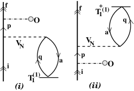
Figure 1: Extra correlation diagrams which appear in the calculation of the polarizabilities using our novel approach. These diagrams do not appear when the CC wave functions are used in the sum-over-the-states method.

We present the static dipole and quadrupole polarizabilities of several important low-lying states of Li in Table 1 and Table 2, respectively. In these Tables, we have also listed other theoretical results and the most recent experimental results, where available. For the ground state, a number of theoretical dipole polarizability results are available, for the excited states, however, few calculations have been carried out. All other theoretical results except one are based on non-relativistic theory. Some of these calculations are also performed using molecular codes, at the cost of atomic symmetries Magnier and Aubert-Frecon (2002). The one available relativistic calculation on the excited states is carried out using a rather approximate method to include the correlation effects due to the Coulomb interaction Ashby and van Wijngaarden (2003b). Our calculation uses a relativistic approach which considers correlation effects to all orders in the form of CC amplitudes.

Figure 2: The correlation diagram that causes a large discrepancy between the calculated and the experimental results of the tensor polarizability of the $2p_{3/2}$ state.

Table 2 shows the result for the static quadrupole polarizabilities. No experimental data is available for comparison, and the available theoretical results for the $2S_{1/2}$ level are not very consistent.

Table 2: The static quadrupole polarizability $\alpha_{2}^{0}$ of many important states in Li [au].

Level	Other theoretical works	This work
	1423a, 1424b,1430c, 1423.266(5)d,
2s ${}^{2}S_{1/2}$	1403e, 1393f, 1424(4)g, 1424.4h	1420
3s ${}^{2}S_{1/2}$	3.5642$\times 10^{5}$h	3.475 $\times 10^{5}$
4s ${}^{2}S_{1/2}$	1.1587$\times 10^{7}$h	1.113$\times 10^{7}$
2p ${}^{2}P_{1/2}$	-	7.804 $\times 10^{4}$
3p ${}^{2}P_{1/2}$	-	$1.033\times 10^{7}$
4p ${}^{2}P_{1/2}$	-	$3.301\times 10^{9}$

^a Spelsberg et al. (1993) Spelsberg et al. (1993), ^b Marinescu et al. (1994) Marinescu et al. (1994), ^c Mérawa et al. (1994) Mérawa et al. (1994), ^d Yan et al. (1996) Yan et al. (1996), ^e,f Patil and Tang (1997,1999) Patil and Tang (1997, 1999), ^g Snow et al. (2005) Snow et al. (2005),

^h Zhang et al. (2007) Zhang et al. (2007).

Table 3: The off-diagonal scalar polarizability in Li [au].

	DF	CCSD(T)
Dipole
$2s-3s$	$-$27.18	$-$20.41
$2s-4s$	$-$202.9	$-$164.2
$3s-4s$	$-$105.8	6.292
Quadrupole
$2s-3s$	2.495 $\times 10^{4}$	2.219$\times 10^{4}$
$2s-4s$	1.245 $\times 10^{5}$	1.134 $\times 10^{5}$
$3s-4s$	9.281 $\times 10^{5}$	6.647 $\times 10^{5}$

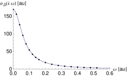
($i$)

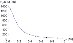
($ii$)

Figure 3: The imaginary parts of the dipole ($i$) and quadrupole ($ii$) polarizabilities of the ground state of Li as a function of the angular frequency $\omega$.

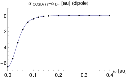
($i$)

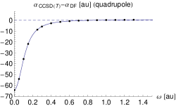
($ii$)

Figure 4: The difference between the DF and CCSD(T) results for the imaginary parts of the dipole ($i$) and quadrupole ($ii$) polarizabilities of the ground state of Li as a function of the angular frequency $\omega$.

Table 4: C₆ and C₈ values for the ground states of Li-Li [au].

	C6($\times 10^{3}$)	C8($\times 10^{5}$)
This work
Dirac-Fock	1.473	0.8891
CCSD(T)	1.396(6)	0.8360
Other theoretical works
Marinescu et al. (1994) Marinescu et al. (1994)	1.388	0.8324
Spelsberg et al. (1996)Spelsberg et al. (1993)
Yan et al. (1996) Yan et al. (1996)	1.39322	0.834258(42)
Patil and Tang (1999) Patil and Tang (1999)	1.360	0.8100
Porsev and Derevianko (2003) Porsev and Derevianko (2003)	-	0.834(4)
Mitroy and Bromley (2003) Mitroy and Bromley (2003)	1.3946	0.83515

Although our method is theoretically superior to the previously employed methods to determine both dipole and quadrupole polarizabilities, it seems that some of the earlier results are in better agreement with the experimental results than ours. This may be due to the fact that experimental energies are used in some of these calculations in contrast to our method which is fully ab initio. This means that in our calculation there may be strong cancelations with neglected higher-order excitations in the correlation effects. We note that in our approach we implicitly take into account certain correlation effects that cannot be accounted for in the usual sum-over-states approach that is used in so many of the earlier calculations. These diagrams, which are shown diagrammatically in Fig. 1, are part of the RPA.

As Table 1 shows, our value for the tensor polarizability of the $2p^{2}P_{3/2}$ level is larger than the experimental result. In our investigation we found that this large value is due to the unusual behavior of the correlation effects produced by the diagram shown in Fig. 2. Leaving out this diagrams yields a value for the tensor polarizability of the $2p^{2}P_{3/2}$ level of $\sim$ 1.6, which agrees nicely with the experiment. For the completeness of the theory this effect cannot be left out. We expect that this effect will cancel with the neglected higher-order excitations.

In Table 3, we present scalar dipole and quadrupole polarizabilities among different $s$-states of Li which are also important in the determination of the van der Waals coefficients of the excited states for ultra-cold atom experiments. Our method can also be employed to determine these quantities in the heavy alkali atoms like Cs and Fr that are important candidates for the study of atomic parity nonconservation Safronova et al. (1999). To our knowledge, no other results are available to compare with these results. As the Table shows, the scalar dipole polarizability between the $2s$ and $3s$ states in Li is of opposite sign to the other alkali atoms Safronova et al. (1999).

Table 5: The triple-dipole constant $v$ for Li-Li-Li ($\times 10^{4}$) [au].

	$v$(Li-Li-Li)
This work
Dirac-Fock	18.576
CCSD(T)	16.934
Other theoretical works
Yan et al. (1996) Yan et al. (1996)	17.0595(6)
Mitroy and Bromley (2003) Mitroy and Bromley (2003)	17.087

The main goal of this work is to illustrate how to evaluate the van der Waals coefficients using the present method. Figure 3 shows the imaginary parts of the dipole and quadrupole polarizabilities (in atomic units) of the ground state of Li as functions of angular frequency, $\omega$. As the Figures show, these quantities fall off exponentially for higher values of $\omega$. To illustrate the effect of electron correlation as a function of frequency, we have plotted the difference between the CCSD(T) and the DF results in Fig. 4. This Figure suggests that the correlation effects vanish for higher frequencies. Using the imaginary parts of the dipole and quadrupole polarizabilities in Eqs. (8), (9) and (10), we evaluated the $C_{6}$, $C_{8}$, and $v$ coefficients, respectively, using a numerical integration method.

In Table 4 we present our $C_{6}$ and $C_{8}$ coefficients and compare them with the other available results. Although our value for the static polarizability of the ground state of Li is slightly smaller than the results presented by others, our $C_{6}$ and $C_{8}$ values are in good agreement with the other results. We present the coefficient $v$ of the third-order correction to the long-range potential in Table 5, which matches well with the other available semi-empirical results.

V Conclusion

We have employed a novel approach to determine both ground and excited states polarizabilities by treating the electron-correlation effects and wave functions due to external operators in the spirit of RCC ansatz. This approach was used to determine the imaginary parts of the polarizabilities which we used to evaluate the van der Waals coefficients of the Li atom. By using this novel technique, we were able to consider the electron-correlation effects rigorously because the technique is fully relativistic and it avoids the sum-over-states method.

VI Acknowledgment

We thank Dr. R. K. Chaudhuri for his contribution in developing some parts of the codes. We thank the C-DAC TeraFlop Super Computing facility, Bangalore, India for the cooperation to carry out these calculations on its computers.

References

- Sahoo (2007) B. K. Sahoo, Chem. Phys. Lett. 448, 144 (2007).
- Greiner et al. (2002) M. Greiner, O. Mandel, T. Esslinger, T. W. Hänsch, and I. Bloch, Nature 415, 39 (2002).
- Moerdijk et al. (1994) A. J. Moerdijk, W. C. Stwalley, R. G. Hulet, and B. J. Verhaar, Phys. Rev. Lett. 72, 40 (1994).
- Quemener et al. (2007) G. Quemener, J. M. Launay, and P. Honvault, Phys. Rev. A 75, 050701 (2007).
- Bourdel et al. (2004) T. Bourdel, L. Khykovich, J. Cubizolles, J. Zhang, F. Chevy, M. Teichmann, L. Tarruell, S. J. Kokkelmans, and C. Salomon, Phys. Rev. Lett. 93, 050401 (2004).
- Taglieber et al. (2008) M. Taglieber, A.-C. Voigt, T. Aoki, T. W. Hänsch, and K. Dieckmann, Phys. Rev. Lett. 100, 010401 (2008).
- Smirnov and Chibisov (1965) B. M. Smirnov and M. I. Chibisov, Sov. Phys. JETP 21, 624 (1965).
- Yan et al. (1996) Z. C. Yan, J. F. Babb, A. Dalgarno, and G. F. W. Drake, Phys. Rev. A 54, 2824 (1996).
- Dalgarno and Davison (1966) A. Dalgarno and W. D. Davison, Adv. At. Mol. Phys. 2, 1 (1966).
- Dalgarno (1967) A. Dalgarno, Adv. Chem. Phys. 12, 143 (1967).
- Boesten et al. (1996) H. M. Boesten, J. M. Vogels, J. G. Tempelaars, and B. J. Verhaar, Phys. Rev. A 54 (1996).
- Amiot et al. (2002) C. Amiot, O. Dulieu, R. F. Gutterres, and F. Masnou-Seeuws, Phys. Rev. A 66, 052506 (2002).
- Dalgarno and Lewis (1955) A. Dalgarno and J. T. Lewis, Proc. R. Soc. London 233, 70 (1955).
- Datta et al. (1995) B. Datta, P. Sen, and D. Mukherjee, J. Phys. Chem. 99, 6441 (1995).
- Kundu and Mukherjee (1991) B. Kundu and D. Mukherjee, Chem. Phys. Lett. 179, 468 (1991).
- Spelsberg et al. (1993) D. Spelsberg, T. Lorenz, and W. Meyer, J. Chem. Phys. 99, 7845 (1993).
- Sahoo et al. (2007a) B. K. Sahoo, B. P. Das, R. K. Chaudhuri, D. Mukherjee, R. G. E. Timmermans, and K. Jungmann, Phys. Rev. A 76, 040504(R) (2007a).