The square-lattice quantum liquid of charge $c$ fermions and spin-neutral two-spinon $s1$ fermions

Abstract

The momentum bands, energy dispersions, and velocities of the charge $c$ fermions and spin-neutral two-spinon $s1$ fermions of a square-lattice quantum liquid referring to the Hubbard model on such a lattice of edge length $L$ in the one- and two-electron subspace are studied. The model involves the effective nearest-neighbor integral $t$ and on-site repulsion $U$ and can be experimentally realized in systems of correlated ultra-cold fermionic atoms on an optical lattice and thus our results are of interest for such systems. Our investigations profit from a general rotated-electron description, which is consistent with the model global $SO(3)\times SO(3)\times U(1)$ symmetry. For the model in the one- and two-electron subspace the discrete momentum values of the $c$ and $s1$ fermions are good quantum numbers so that in contrast to the original strongly-correlated electronic problem their interactions are residual. The use of our description renders an involved many-electron problem into a quantum liquid with some similarities with a Fermi liquid. For the Hubbard model on a square lattice in the one- and two-electron subspace a composite $s1$ fermion consists of a spin-singlet spinon pair plus an infinitely thin flux tube attached to it. In the $U/4t\rightarrow\infty$ limit of infinite on-site interaction the $c$ fermions become non-interacting spinless fermions and the $s1$ fermion occupancy configurations that generate the spin degrees of freedom of spin-density $m=0$ ground states become within a suitable mean-field approximation for the fictitious magnetic field $B_{s1}\,{\vec{e}}_{x_{3}}$ brought about by the correlations of the original $N$ electron problem those of a full lowest Landau level with $N/2$ degenerate one-$s1$ fermion states of the two-dimensional quantum Hall effect. In turn, for $U/4t$ finite the degeneracy of the $N/2$ one-$s1$-fermion states is removed by the emergence of a finite-energy-bandwidth $s1$ fermion dispersion yet the number of $s1$ band discrete momentum values remains being given by $B_{s1}\,L^{2}/\Phi_{0}$ and the $s1$ effective lattice spacing by $a_{s1}=l_{s1}/\sqrt{2\pi}$ where $l_{s1}$ is the fictitious-magnetic-field length and in our units the fictitious-magnetic-field flux quantum reads $\Phi_{0}=1$. Elsewhere it is found that the use of the square-lattice quantum liquid of charge $c$ fermions and spin-neutral two-spinon $s1$ fermions investigated here contributes to the further understanding of the role of electronic correlations in the unusual properties of the hole-doped cuprate superconductors. This indicates that quantum-Hall-type behavior with or without magnetic field may be ubiquitous in nature.

I Introduction

The Hubbard model on a square lattice is the simplest realistic toy model for description of the electronic correlation effects in general many-electron problems with short-range interaction on such a lattice and therefore is the obvious starting point for the study of the role of such effects in the exotic physics of the hole-doped cuprates two-gaps ; k-r-spaces ; duality ; 2D-MIT ; Basov ; ARPES-review ; Tsuei ; pseudogap-review . The model involves two effective parameters: the in-plane nearest-neighbor transfer integral $t$ and the effective on-site repulsion $U$. Despite that it is among the mostly studied models in condensed matter physics, there is no exact solution and few controlled approximations exist for finite $U/4t$ values.

In this paper we study the momentum bands, energy dispersions, and velocities of the charge $c$ fermions and spin-neutral two-spinon $s1$ fermions introduced for the model on the square lattice in Ref. companion . The $s1$ fermions emerge from the spin-neutral two-spinon $s1$ bond particles companion ; s1-bonds through an extended Jordan-Wigner transformation J-W ; Fradkin ; Wang ; Feng . Our study has as starting point the properties of the Hubbard model on the square lattice in the one- and two-electron subspace defined in Ref. companion and profits from the general rotated-electron description introduced in that reference.

There is consensus about the scientific interest of the Hubbard model on the square lattice as simplest toy model for describing the effects of electronic correlations in the high-$T_{c}$ superconductors two-gaps ; k-r-spaces ; duality ; 2D-MIT ; Basov ; ARPES-review ; Tsuei ; pseudogap-review and their Mott-Hubbard insulators parent compounds Cuprates-insulating-phase ; LCO-neutr-scatt . However, many open questions about its properties remain unsolved. Interestingly, the model can be experimentally realized with unprecedented precision in systems of correlated ultra-cold fermionic atoms on an optical lattice Zoller and one may expect very detailed experimental results over a wide range of parameters to be available.

The square-lattice quantum liquid of charge $c$ fermions and spin-neutral two-spinon $s1$ fermions and the related general rotated-electron description of Ref. companion are consistent with the global $SO(3)\times SO(3)\times U(1)=[SO(4)\times U(1)]/Z_{2}$ symmetry found recently in Ref. bipartite for the model on any bipartite lattice. Such a global symmetry is an extension of the $SO(4)$ symmetry known to occur for the model on such lattices HL ; Zhang . The extended global symmetry is related to the rotated electrons, which for on-site repulsion $U>0$ emerge from the the electrons through a unitary transformation of the type considered in Ref. Stein , and to the local symmetries and unitary transformations studied in Ref. U(1)-NL .

The building blocks of the general description introduced in Ref. companion are the $\eta$-spin-$1/2$ $\eta$-spinons, spin-$1/2$ spinons, and spinless and $\eta$-spinless charge $c$ fermions whose occupancy configurations generate the state representations of the $\eta$-spin $SU(2)$ symmetry, spin $SU(2)$ symmetry, and $U(1)$ symmetry, respectively, associated with the model global $SO(3)\times SO(3)\times U(1)=[SU(2)\times SU(2)\times U(1)]/Z_{2}^{2}$ symmetry. Such three basic objects are well defined for $U>0$. These state representations are found in Ref. companion to correspond to a complete set of momentum eigenstates. The $\eta$-spin-$1/2$ $\eta$-spinons describe the $\eta$-spin degrees of freedom of the rotated-electron occupancy configurations that generate such states involving doubly occupied and unoccupied sites, the spin-$1/2$ spinons the spin degrees of freedom of the rotated-electron configurations of the singly occupy sites, and the $c$ fermions the charge excitations associated with rotated-electron motion that conserves the numbers of singly occupied, doubly occupied, and unoccupied sites.

For $U/4t\gg 1$ the $c$ fermion, spinon, and $\eta$-spinon operators become the quasicharge, spin, and pseudospin operators, respectively, obtained from the transformation considered in Ref. Ostlund-06 , which does not introduce Hilbert-space constraints. Such quasicharge, spin, and pseudospin operators have for $U/4t\gg 1$ the same expressions in terms of creation and annihilation electron operators as the $c$ fermion, spinon, and $\eta$-spinon operators for $U>0$ in terms of rotated-electron creation and annihilation operators. The unitary character of the transformation between electrons and rotated electrons then assures that the transformation that generates the $c$ fermion, spinon, and $\eta$-spinon operators from the electronic operators also does not introduce Hilbert-space constraints. The vacuum of the theory is given in Eq. (154) of Appendix A, where some basic information on the square-lattice quantum liquid one- and two-electron subspace defined in Ref. companion is provided. There is a vacuum of general form given in that equation for each subspace with a constant finite value $2S_{c}$ for the number of rotated electrons that singly occupy sites. $S_{c}$ is also the eigenvalue of the generator of the hidden charge $U(1)$ global symmetry bipartite . For both the model on the square and one-dimensional (1D) lattice such a $S_{c}>0$ vacuum is invariant under the electron - rotated-electron unitary transformation.

For the square-lattice quantum liquid associated with the Hubbard model in the one- and two-electron subspace only the charge $c$ fermions and spin-neutral two-spinon $s1$ bond particles play an active role companion ; s1-bonds . In contrast to previous descriptions involving Jordan-Wigner transformations Wang ; Feng or slave-boson representations 2D-MIT ; Fazekas ; Xiao-Gang and referring to the model for large values of the on-site repulsion $U$ or Heisenberg and $t-J$ models, whose spinless fermions arise from spin-$1/2$ objects, the $s1$ fermions emerge from hard-core spin-neutral two-spinon composite objects and are well defined for finite $U$ values of the on-site repulsion. As mentioned above, the spin-$1/2$ spinons are the spins of the rotated electrons that singly occupied lattice sites and emerge from a suitably electron - rotated-electron unitary transformation introduced in Ref. companion . Therefore, here the single-occupancy constraint is naturally fulfilled.

For the Hubbard model on the square lattice in the one- and two-electron subspace as defined in that reference there are no $\alpha\nu$ fermions other than none or one zero-momentum $s2$ fermion and $[S_{c}-S_{s}]$ or $[S_{c}-S_{s}-2]$ $s1$ fermions, respectively, where $S_{s}$ denotes the spin. The interest of the description introduced in Ref. companion lies in the fact that for the subspaces of the one- and two-electron subspace spanned by mutually neutral states where the $s1$ fermion operators act onto, the two $s1$ translation generators $\vec{q}_{s1\,x_{1}}$ and $\vec{q}_{s1\,x_{2}}$ in the presence of the fictitious magnetic field ${\vec{B}}_{s1}$ associated with the $s1$ fermion Jordan-Wigner transformation commute with each other and with both the Hamiltonian and momentum operator. In contrast, the Hubbard model on the square lattice in the whole Hilbert space does not commute with such translation generators companion . Therefore, for the square-lattice quantum liquid corresponding to the Hubbard model on a square lattice in the one- and two-electron subspace the $s1$ fermion discrete momentum values $\vec{q}_{j}=[{q_{j}}_{x_{1}},{q_{j}}_{x_{2}}]$ are good quantum numbers. Here ${q_{j}}_{x_{1}}$ and ${q_{j}}_{x_{2}}$ are eigenvalues of the two $s1$ translation generators $\vec{q}_{s1\,x_{1}}$ and $\vec{q}_{s1\,x_{2}}$, respectively. In addition, the description of Ref. companion has been constructed to inherently the $c$ fermion discrete momentum values being good quantum numbers for the whole Hilbert space. In turn, our method involves approximations to derive the shape of the $s1$ momentum band boundary and the form of the $c$ and $s1$ fermion energy dispersions. The fulfillment of such tasks is the main goal of this paper. For the 1D model the discrete momentum values of the $c$ and $s1$ fermions in units of $2\pi/L$ are quantum numbers of the exact solution companion . For the model on the square lattice the nearest-neighboring components of the $c$ and $s1$ discrete momentum values $\vec{q}_{j}=[{q_{j}}_{x_{1}},{q_{j}}_{x_{2}}]$ are such that $[{q_{j}}_{xi}-{q_{j^{\prime}}}_{xi}]=2\pi/L$ where $i=1$ or $i=2$ and the indices $j$ and $j^{\prime}$ refer to nearest neighboring discrete momentum values. The shape of the $c$ band is that of the first Brillouin zone. Hence the main open issue is the shape of the $s1$ boundary line for $x\geq 0$ and $m=0$ ground states, and that along with the $c$ and $s1$ fermion energy dispersions is one of the problems studied in this paper.

It follows from the results of Ref. companion that for the Mott-Hubbard insulator at hole concentration $x=0$ and spin density $m=0$ both the $c$ and $s1$ bands are full. For the Hubbard model on a square-lattice the $c$ band has for all energy eigenstates the same momentum area and shape as the electronic first Brillouin zone. For $m=0$ ground states with a small finite hole concentration $x$ there arises a circular $c$ Fermi line around $-\vec{\pi}=-[\pi,\pi]$ of ratio $\approx\sqrt{x\pi}\,2$, which encloses a $c$ fermion unfilled momentum area $x\,4\pi^{2}$. Since the $c$ effective lattice equals the original lattice and thus its spacing $a_{c}$ equals the original lattice constant $a$, the $c$ fermion occupancy configurations that generate the energy eigenstates conserve translational invariance.

In turn, consistently with the ground-state $s1$ effective-lattice occupancies of Ref. companion , for $x\geq 0$ and $m=0$ ground states the $s1$ band is full. For the $x=0$ and $m=0$ absolute ground state that band has a momentum area $2\pi^{2}$ and is found in this paper to coincide with an antiferromagnetic reduced Brillouin zone such that $|q_{x_{1}}|+|q_{x_{2}}|\leq\pi$, which is enclosed by a boundary whose momenta ${\vec{q}}_{Bs1}$ belong to the lines connecting $[\pm\pi,0]$ and $[0,\pm\pi]$. Such a $s1$ band shape and momentum area are consistent with the result of Ref. companion that at $x=0$ and $m=0$ the square $s1$ effective lattice has spacing $a_{s1}=\sqrt{2}\,a$. Indeed our studies confirm that its periodicity has increased relative to that of the original lattice owing to the appearance of a long-range antiferromagnetic order. Moreover, we find that the Fermi line has for the $x=0$ and $m=0$ ground state the same form as the $s1$ boundary line so that it refers to the lines connecting $[\pm\pi,0]$ and $[0,\pm\pi]$. For very small values of $x$, both the momentum areas enclosed by the $s1$ boundary line and the Fermi line decrease to $(1-x)2\pi^{2}$. Then the latter line becomes hole like and both such lines remain near the lines connecting $[\pm\pi,0]$ and $[0,\pm\pi]$. This is consistent with the recent experimental results of Ref. k-r-spaces , which reveal that for small hole concentrations the momentum-space region near such lines plays a major role in the Fermi-line physics of the hole-doped cuprate superconductors.

Upon further increasing the hole concentration $x$ the $s1$ momentum band remains full for $x\geq 0$ and $m=0$ ground states and encloses a smaller momentum area $(1-x)2\pi^{2}$, alike for small $x$. For $0<x<x_{*}$ and $m=0$ there is a short-range spin order. Here $x_{*}\in(0.23,0.28)$ for approximately $u_{0}\leq U/4t\leq u_{1}$ where $u_{0}\approx 1.3$ and $u_{1}\approx 1.6$ is a critical concentration $x_{*}$ introduced in Subsection IV-F, below which such an order prevails. For $0<x\ll 1$ it is a short-range incommensurate-spiral spin order, consistently with the spacing of the square $s1$ effective lattice reading $a_{s1}=\sqrt{2/(1-x)}\,a$. Such and related types of spin orders have been observed in the cuprate superconductors nematic-order ; spiral-order . The schemes introduced in Refs. cuprates0 ; cuprates involve modified versions of the square-lattice quantum liquid investigated in this paper and contribute to the further understanding of the unusual properties of the hole-doped cuprate superconductors Kam ; PSI-ANI-07 ; LSCO-resistivity ; Y-resistivity .

Our study focus on the Hubbard model on the square lattice. The reason why often our analysis refers to the same model on the 1D lattice as well is that in contrast to real-space dimensions $D>1$ there is an exact solution for 1D Lieb ; Takahashi ; Martins . In spite of then the model referring to a qualitatively different physics, our quantum-object description also applies to 1D. For instance, in the $U/4t\rightarrow\infty$ limit the $c$ fermions become both for the model on a 1D and square lattices non-interacting spinless fermions. In turn, the $s1$ fermion occupancy configurations that generate the spin degrees of freedom of spin-density $m=0$ ground states become in that limit for 1D and the square lattice those of the spins of the spin-charge factorized wave function introduced both by Woynarovich Woy and Ogata and Shiba Ogata and within a suitable mean-field approximation for a fictitious magnetic field brought about by the electronic correlations those of a full lowest Landau level with $N_{s1}=N_{a_{s1}}^{2}=N/2$ one-$s1$-fermion degenerate states of the 2D quantum Hall effect (QHE), respectively. Here $N_{a_{s1}}^{2}$ is the number of both sites of the square $s1$ effective lattice and $s1$ band discrete momentum values.

Consistently with the validity of the $c$ fermion, $2\nu$-$\eta$-spinon $\eta\nu$ fermion, and $2\nu$-spinon $s\nu$ fermion description of Ref. companion where $\nu=1,2,...$ gives the number of $\eta$-spinon or spinon pairs, which for the model in the one- and two-electron subspace considered in this paper involves only the $c$ fermions and composite two-spinon $s1$ fermions, it is shown in that reference that for 1D and the limit $N_{a}\gg 1$, which such a description refers to, the discrete momentum values of the $c$ fermions and $\alpha\nu$ fermions where $\alpha=\eta,s$ coincide with the quantum numbers of the exact solution.

In contrast to the original strongly-correlated electron problem, the interactions of the $c$ and $s1$ fermions are residual owing to their momentum values being good quantum numbers. Consistently, the non-perturbative and involved problem concerning the effects of the electronic correlations of the Hubbard model on the square lattice simplifies when expressed in terms of the $c$ and $s1$ fermion residual interactions. Our results and those of Ref. cuprates0 reveal that for the model on that lattice the residual interactions recombine the charge and spin degrees of freedom to such an extent that one cannot speak of a spin-charge separation as that occurring in 1D. For instance, one cannot express the electronic spectral functions as a simple convolution of $c$ fermion and $s1$ fermion spectral functions. Therefore, the concept of spin-charge separation does not apply to the model on the square lattice, at least with the meaning it has in 1D correlated systems.

The square-lattice quantum liquid studied in this paper is non-perturbative in terms of electron operators so that, in contrast to a 3D isotropic Fermi liquid Landau ; Pines , rewriting its theory in terms of the standard formalism of many-electron physics is an extremely complex problem. Fortunately, the description of the physics of such a quantum liquid simplifies when it is expressed in terms of the $c$ and $s1$ fermion operators. In the $x>0$ studies of Refs. cuprates0 ; cuprates the effects of the residual interactions of the $c$ and $s1$ fermions play a major role. At $x=0$ the residual interactions of the $s1$ fermions have no direct effects on the spin spectrum. Within the operator description used in this paper the study of the $x=0$ spin spectrum refers to an effectively non-interacting problem. In turn, in terms of electrons it is an involved many-body problem. The studies of Subsection VI-B confirm the validity of our description for the model on the square lattice: At $x=0$ our analytical expressions for the spin-wave dispersion, which corresponds to the coherent part of the $x=0$ spin spectrum, fully agree with the controlled numerical results of Ref. LCO-Hubbard-NuMi , obtained by summing up an infinite set of electronic ladder diagrams. Moreover, an excellent quantitative agreement with the inelastic neutron scattering of the La_2-xSr_xCuO₄ (LSCO) Mott-Hubbard insulator parent compound La₂CuO₄ (LCO) LCO-neutr-scatt is reached.

The paper is organized as follows. The model, its $c$ and $s1$ fermion description and related rotated-electron representation, the limitations and advantages of such a description, and the emergence of the $s1$ fermions from the hard-core spin-neutral two-spinon $s1$ bond particles are the subjects of Section II. In Section III further evidence is provided that for the Hubbard model on the square lattice in the one- and two-electron subspace the $c$ and $s1$ band discrete momentum values are good quantum numbers, consistently with the results of Ref. companion on that issue. In addition, the Fermi line is expressed in terms momenta belonging to the $c$ Fermi line and $s1$ boundary line and its anisotropy is investigated. The derivation of the $c$ and $s1$ fermion energy dispersions of the square-lattice quantum liquid first-order energy functional associated with the ground-state normal-ordered Hamiltonian of the Hubbard model in the one- and two-electron subspace is the subject of Section IV. The $c$ and $s1$ fermion velocities and analysis of their relation to the velocities associated with the one- and two-electron excitations is the subject of Section V. Section VI presents a brief discussion concerning the combination of the $c$ and $s1$ fermion description with the exact Bethe-ansatz solution to study the dynamical and correlation functions of the 1D Hubbard model. Moreover, in that section we study the spin excitations of the half-filling Hubbard model on the square lattice and find excellent agreement between the results obtained by use of the square-lattice quantum liquid of $c$ and $s1$ fermions and the standard formalism of many-electron physics LCO-Hubbard-NuMi . Finally, the concluding remarks are presented in Section VII.

II The model and the $c$ and $s1$ fermion description

Here we address the problem of the description of the Hubbard model on a square lattice in the one- and two-electron subspace in terms of charge $c$ fermions and spin-singlet two-spinon $s1$ fermions introduced in Ref. companion . In that subspace the model refers to the square-lattice quantum liquid, which is expected to refer to a wider class of many-electron problems with short-range interactions on the square lattice belonging to the same universality class. We start by introducing the model, its global symmetry, and the rotated-electron representation and discuss the limitations and advantages of the corresponding $c$ and $s1$ fermion description.

II.1 The Hubbard model and its global symmetry, rotated electrons, and the limitations of our description

The Hubbard model on the two-dimensional (2D) square lattice with torus periodic boundary conditions and the same model on the 1D lattice with periodic boundary conditions, spacing $a$, $N_{a}^{D}\equiv[N_{a}]^{D}$ sites where $D=1$ and $D=2$ for the 1D and square lattices, respectively, $N_{a}^{D}\gg 1$ even and large, and lattice edge length $L=N_{a}\,a$ for 2D and chain length $L=N_{a}\,a$ for 1D is given by,

$$\hat{H}=-t\sum_{\langle\vec{r}_{j}\vec{r}_{j^{\prime}}\rangle}\sum_{\sigma=\uparrow,\downarrow}[c_{\vec{r}_{j},\sigma}^{{\dagger}}\,c_{\vec{r}_{j^{\prime}},\sigma}+h.c.]+U\,[N_{a}^{D}-\hat{Q}]/2\,.$$ (1)

Here ${\langle\vec{r}_{j}\vec{r}_{j^{\prime}}\rangle}$ refers to nearest neighboring sites, the operator $c_{\vec{r}_{j},\sigma}^{{\dagger}}$ creates an electron of spin projection $\sigma$ at the site of real-space coordinate $\vec{r}_{j}$, and the operator,

$${\hat{Q}}=\sum_{j=1}^{N_{a}^{D}}\sum_{\sigma=\uparrow,\downarrow}\,n_{\vec{r}_{j},\sigma}\,(1-n_{\vec{r}_{j},-\sigma})\,,$$ (2)

where $n_{{\vec{r}}_{j},\sigma}=c_{\vec{r}_{j},\sigma}^{{\dagger}}c_{\vec{r}_{j},\sigma}$ and $-\sigma=\uparrow$ (and $-\sigma=\downarrow$) for $\sigma=\downarrow$ (and $\sigma=\uparrow$) counts the number of electron singly occupied sites. Hence the operator ${\hat{D}}=[{\hat{N}}-{\hat{Q}}]/2$ counts the number of electron doubly occupied sites where ${\hat{N}}=\sum_{\sigma}{\hat{N}}_{\sigma}$ and ${\hat{N}}_{\sigma}=\sum_{j=1}^{N_{a}^{D}}n_{{\vec{r}}_{j},\sigma}$. We denote the $\eta$-spin (and spin) value of the energy eigenstates by $S_{\eta}$ (and $S_{s}$) and the corresponding projection by $S^{z}_{\eta}=-[N_{a}^{D}-N]/2$ (and $S^{z}_{s}=-[N_{\uparrow}-N_{\downarrow}]/2$). We focus our attention onto initial ground states with a hole concentration $x=[N_{a}^{D}-N]/N_{a}^{D}\geq 0$ and spin density $m=[N_{\uparrow}-N_{\downarrow}]/N_{a}^{D}=0$ and their excited states belonging to the one- and two-electron subspace defined in Ref. companion .

The unitary operator $\hat{V}=\hat{V}(U/4t)$ associated with the electron - rotated-electron unitary transformation plays a key role in the construction of the general description of the Hubbard model on a square lattice introduced in Ref. companion . Out of the manyfold of unitary operators of Refs. Stein ; bipartite , the studies of that paper consider a unique choice for ${\hat{V}}={\hat{V}}(U/4t)$ such that the states $|\Psi_{U/4t}\rangle={\hat{V}}^{{\dagger}}|\Psi_{\infty}\rangle$ are energy and momentum eigenstates for $U/4t>0$. It corresponds to a suitable chosen set $\{|\Psi_{\infty}\rangle\}$ of $U/4t\rightarrow\infty$ energy eigenstates. The states $|\Psi_{U/4t}\rangle={\hat{V}}^{{\dagger}}|\Psi_{\infty}\rangle$ (one for each value of $U/4t>0$) that are generated from the same initial state $|\Psi_{\infty}\rangle$ belong to the same $V$ tower. The generator ${\tilde{S}}_{c}$ of the hidden $U(1)$ symmetry of the global $SO(3)\times SO(3)\times U(1)=[SO(4)\times U(1)]/Z_{2}$ symmetry found for the $U/4t>0$ Hubbard model on a square lattice in Ref. bipartite reads ${\tilde{S}}_{c}={\hat{V}}^{{\dagger}}\,{\hat{S}}_{c}\,{\hat{V}}$ where ${\hat{S}}_{c}={\hat{Q}}/2$ and the operator ${\hat{Q}}$ is given in Eq. (2). Its eigenvalue $S_{c}$ equals one-half the number of rotated-electron singly occupied sites $2S_{c}$. The unitary transformation associated with the operator ${\hat{V}}^{{\dagger}}$ maps the electron operators $c_{\vec{r}_{j},\sigma}^{{\dagger}}$ and $c_{\vec{r}_{j},\sigma}$ onto rotated-electron creation and annihilation operators ${\tilde{c}}_{\vec{r}_{j},\sigma}^{{\dagger}}={\hat{V}}^{{\dagger}}\,c_{\vec{r}_{j},\sigma}^{{\dagger}}\,{\hat{V}}$ and ${\tilde{c}}_{\vec{r}_{j},\sigma}={\hat{V}}^{{\dagger}}\,c_{\vec{r}_{j},\sigma}\,{\hat{V}}$, respectively. In terms of the latter operators the expression of the generator whose application onto the $N=0$ and $S_{c}=0$ electron vacuum generates the energy eigenstates $|\Psi_{U/4t}\rangle$ belonging to the same $V$ tower are the same for the whole range of $U/4t>0$ values: It has the same expression as the generator of the initial state $|\Psi_{\infty}\rangle$ in terms of electron creation and annihilation operators. (The $N=0$ and $S_{c}=0$ electron vacuum corresponds to that of Eq. (154) of Appendix A for $N_{a_{\eta}}^{D}=N_{a}^{D}$ and $N_{a_{s}}^{D}=2S_{c}=0$.)

However, for $U/4t>0$ (and $U/4t\rightarrow\infty$) the expression of the generators of the energy eigenstates from the electron vacuum are very complex in terms of rotated-electron (and electron) operators. Indeed, those are not the ultimate objects whose occupancy configurations that generate such states have a simple expression. The studies of Ref. companion considered a complete set $\{|\Phi_{U/4t}\rangle\}$ of general momentum eigenstates $|\Phi_{U/4t}\rangle={\hat{V}}^{{\dagger}}|\Phi_{\infty}\rangle$ given in Eq. (157) of Appendix A. On the right-hand side of that equation the lowest-weight-state (LWS) momentum eigenstates $|\Phi_{LWS;U/4t}\rangle$ are those given in Eq. (158) of such an Appendix. These states can be generated from corresponding $U/4t\rightarrow\infty$ momentum eigenstates as $|\Phi_{U/4t}\rangle={\hat{V}}^{{\dagger}}|\Phi_{\infty}\rangle$. Moreover, $|\Phi_{LWS;U/4t}\rangle={\hat{V}}^{{\dagger}}|\Phi_{LWS;\infty}\rangle$ where ${\hat{V}}^{{\dagger}}$ is the electron - rotated-electron unitary operator that also generates the energy and momentum eigenstates $|\Psi_{U/4t}\rangle={\hat{V}}^{{\dagger}}|\Psi_{\infty}\rangle$ from the corresponding $U/4t\rightarrow\infty$ energy and momentum eigenstates $|\Psi_{\infty}\rangle$.

The generators onto the vacuum of Eq. (154) of Appendix A of the LWS momentum eigenstates $|\Phi_{LWS;U/4t}\rangle$ are Slatter-determinant products of $c$ and $\alpha\nu$ fermion creation operators. For the 1D Hubbard model one has that $|\Phi_{U/4t}\rangle=|\Psi_{U/4t}\rangle$ so that the states $|\Phi_{U/4t}\rangle$ of Eq. (157) of Appendix A are both momentum and energy eigenstates whereas for the model on the square lattice the energy and momentum eigenstates $|\Psi_{U/4t}\rangle={\hat{V}}^{{\dagger}}|\Psi_{\infty}\rangle$ are a superposition of a well-defined set of momentum eigenstates $|\Phi_{U/4t}\rangle={\hat{V}}^{{\dagger}}|\Phi_{\infty}\rangle$ with the same momentum eigenvalue, values of $S_{\eta}$, $S_{\eta}^{z}$, $S_{s}$, $S_{s}^{z}$, $S_{c}$, $C_{\eta}=\sum_{\nu}\nu\,N_{\eta,\nu}$, $C_{s}=\sum_{\nu}\nu\,N_{s,\nu}$, and $c$ fermion momentum distribution function $N_{c}({\vec{q}})$ companion . In some cases that set of states refers to a single state so that $|\Psi_{U/4t}\rangle=|\Phi_{U/4t}\rangle$ and the state $|\Phi_{U/4t}\rangle$ under consideration is both an energy and momentum eigenstate. This is so for the momentum eigenstates $|\Phi_{U/4t}\rangle$ that span the one- and two-electron subspace as defined in Ref. companion . That $|\Phi_{U/4t}\rangle=|\Psi_{U/4t}\rangle$ for the 1D Hubbard model in the whole Hilbert space follows from its integrability being for $N_{a}\gg 1$ associated with an infinite number of conservation laws Martins . According to the results of Ref. Prosen such laws are equivalent to the independent conservation of the set of numbers $\{N_{\alpha\nu}\}$ of $\alpha\nu$ fermions, which for that model are good quantum numbers.

The $\alpha\nu$ fermion operators $f_{\vec{q}_{j},\alpha\nu}^{{\dagger}}$ appearing in the Slatter-determinant products of the LWS momentum eigenstates $|\Phi_{LWS;U/4t}\rangle$ given in Eq. (158) of Appendix A correspond to an independent problem in each subspace with constant values of $S_{c}$, $S_{s}$, and number $N_{a_{\alpha\nu}}^{D}=[N_{\alpha\nu}+N^{h}_{\alpha\nu}]$ of both sites of the $\alpha\nu$ effective lattice and discrete momentum values of the $\alpha\nu$ band. The operators $f_{\vec{q}_{j},\alpha\nu}^{{\dagger}}$ and $f_{\vec{q}_{j},\alpha\nu}$ act on subspaces spanned by mutually neutral states, which are transformed into each other by $\alpha\nu$ fermion particle-hole processes. As discussed in Ref. companion , that assures that for the model on the square lattice the components $q_{x_{1}}$ and $q_{x_{2}}$ of the microscopic momenta $\vec{q}=[q_{x_{1}},q_{x_{2}}]$ refer to commuting $s1$ translation generators $\hat{q}_{s1\,x_{1}}$ and $\hat{q}_{s1\,x_{2}}$. In turn, for the operators $f_{\vec{q}_{j},c}^{{\dagger}}$ appearing in the Slatter-determinant products of the LWS momentum eigenstates there are in 1D two types of quantum problems depending on the even or odd character of the number $[B_{\eta}+B_{s}]=\sum_{\alpha\nu}N_{\alpha\nu}$. Indeed, in spite of the $c$ effective lattice being identical to the original lattice, both for the model on the 1D and square lattices the $c$ fermions feel the Jordan-Wigner phases of the $\alpha\nu$ fermions created or annihilated under subspace transitions that do not conserve the number $[B_{\eta}+B_{s}]=\sum_{\alpha\nu}N_{\alpha\nu}$.

The $\alpha\nu$ fermion operators $f^{{\dagger}}_{{\vec{q}},\alpha\nu}$ and $f_{{\vec{q}},\alpha\nu}$ act onto subspaces spanned by neutral states. Creation of one $\alpha\nu$ fermion is however a well-defined process whose generator is the product of an operator that fulfills small changes in the $\alpha\nu$ effective lattice and corresponding $\alpha\nu$ momentum band and the operator $f^{{\dagger}}_{{\vec{q}},\alpha\nu}$ suitable to the excited-state subspace. In the Slatter-determinant products of Eq. (158) of Appendix A it is implicitly assumed that the $\alpha\nu$ momentum bands are those of the state under consideration so that the corresponding generators on the vacua are simple products of $f^{{\dagger}}_{{\vec{q}},\alpha\nu}$ operators. The $c$ effective lattice and number $N_{a}^{D}$ of $c$ band discrete momentum values remain unaltered for the whole Hilbert space. In turn, concerning transitions between subspaces with slightly different discrete values for such momenta again creation or annihilation of one $c$ fermion is a well-defined process whose generator is the product of an operator that fulfills the corresponding small changes in the $c$ momentum band and the operator $f^{{\dagger}}_{{\vec{q}},c}$ or $f_{{\vec{q}},c}$, respectively, appropriate to the excited-state subspace.

Following the results of Ref. companion , the bad news is that for the Hubbard model on the square lattice the microscopic momenta carried by the $\alpha\nu$ fermions are not in general good quantum numbers, in contrast to the integrable 1D Hubbard model. That results from the lack of integrability of the Hubbard model on the square lattice, which is behind the set of numbers $\{N_{\alpha\nu}\}$ of $\alpha\nu$ fermions not being in general conserved, yet the numbers $C_{\eta}=\sum_{\nu}\nu\,N_{\eta,\nu}$ and $C_{s}=\sum_{\nu}\nu\,N_{s,\nu}$ and the $c$ fermion momentum distribution function $N_{c}({\vec{q}})$ are. It follows that for the model on the square lattice the generators onto the vacuum of Eq. (154) of Appendix A of the energy and momentum eigenstates are not simple Slatter-determinant products of $c$ and $\alpha\nu$ fermion creation operators as those of Eq. (158) of Appendix A and such states are in general different from the momentum eigenstates $|\Phi_{U/4t}\rangle={\hat{V}}^{{\dagger}}|\Phi_{\infty}\rangle$. The good news is that for the model on the square lattice in the one- and two-electron subspace defined in Ref. companion one has that $N_{\alpha\nu}=0$ except for the $\alpha\nu=s1$ and $\alpha\nu=s2$ fermion branches and owing to symmetries specific to that subspace $N_{s1}=[S_{c}-S_{s}-2N_{s2}]$ and $N_{s2}=0,1$ are conserved so that the microscopic momenta of the $s1$ fermions are good quantum numbers and the states $|\Phi_{U/4t}\rangle=|\Psi_{U/4t}\rangle$ are energy eigenstates.

Addition of chemical-potential and magnetic-field operator terms to the Hamiltonian (1) lowers its symmetry. A property of key importance follows from such operator terms commuting with that Hamiltonian. Such a property reveals that the $c$ fermion and $\alpha\nu$ fermion occupancy configurations and independent $\eta$-spinon and spinon occupancies that generate the $4^{N_{a}^{D}}$ momentum eigenstates $|\Phi_{U/4t}\rangle={\hat{V}}^{{\dagger}}|\Phi_{\infty}\rangle$ of general form given in Eq. (157) of Appendix A correspond to state representations of the $SO(3)\times SO(3)\times U(1)$ group for all values of the densities $n=(1-x)$ and $m$, as confirmed explicitly in Ref. companion .

The unitary operator ${\hat{V}}$ commutes with the momentum operator $\hat{\vec{P}}$, three generators of the spin $SU(2)$ symmetry, and three generators of the $\eta$-spin $SU(2)$ symmetry bipartite ; companion . These two $SU(2)$ symmetries are contained in the model global $SO(3)\times SO(3)\times U(1)=[SU(2)\times SU(2)\times U(1)]/Z_{2}^{2}$ symmetry. Hence, the momentum operator and such six generators have the same expression in terms of electron and rotated-electron creation and annihilation operators. In contrast, the generator ${\tilde{S}}_{c}$ of the $U(1)$ symmetry also contained in that global symmetry and the Hamiltonian (1) do not commute with such a unitary operator.

The general rotated-electron description introduced in Ref. companion associates with any operator ${\hat{O}}$ a rotated operator ${\tilde{O}}={\hat{V}}^{{\dagger}}\,{\hat{O}}\,{\hat{V}}$, which has the same expression in terms of rotated-electron creation and annihilation operators as ${\hat{O}}$ in terms of electron creation and annihilation operators, respectively. Any operator ${\hat{O}}$ expressed in terms of electron creation and annihilation operators can then be written in terms of rotated-electron creation and annihilation operators as,

$${\hat{O}} = {\hat{V}}\,{\tilde{O}}\,{\hat{V}}^{{\dagger}}={\tilde{O}}+[{\tilde{O}},\,{\hat{S}}\,]+{1\over 2}\,[[{\tilde{O}},\,{\hat{S}}\,],\,{\hat{S}}\,]+...={\tilde{O}}+[{\tilde{O}},\,{\tilde{S}}\,]+{1\over 2}\,[[{\tilde{O}},\,{\tilde{S}}\,],\,{\tilde{S}}\,]+...\,,$$

$${\hat{S}} = -{t\over U}\,\left[\hat{T}_{+1}-\hat{T}_{-1}\right]+{\cal{O}}(t^{2}/U^{2})\,;\hskip 7.11317pt{\tilde{S}}=-{t\over U}\,\left[\tilde{T}_{+1}-\tilde{T}_{-1}\right]+{\cal{O}}(t^{2}/U^{2})\,.$$ (3)

The operator $\hat{S}$ appearing in this equation is such that ${\hat{V}}^{{\dagger}}=e^{{\hat{S}}}$, ${\hat{V}}=e^{-{\hat{S}}}$, and then $[\hat{S},{\hat{V}}]=0$ and $\hat{S}=\tilde{S}$. The expression of ${\hat{S}}$ involves only the kinetic operators $\hat{T}_{0}$, $\hat{T}_{+1}$, and $\hat{T}_{-1}$ so that that of ${\tilde{S}}$ involves only the rotated kinetic operators $\tilde{T}_{0}$, $\tilde{T}_{+1}$, and $\tilde{T}_{-1}$. The former kinetic operators are related to the kinetic-energy operator $t\,\hat{T}=-t\sum_{\langle\vec{r}_{j}\vec{r}_{j^{\prime}}\rangle}\sum_{\sigma=\uparrow,\downarrow}[c_{\vec{r}_{j},\sigma}^{{\dagger}}\,c_{\vec{r}_{j^{\prime}},\sigma}+h.c.]$ of the Hamiltonian (1), which can be expressed as $\hat{T}=\hat{T}_{0}+\hat{T}_{+1}+\hat{T}_{-1}$. (The expressions of the three kinetic operators are provided in Ref. companion .) The operator $\hat{T}_{0}$ does not change electron double occupancy. In turn, the operators $\hat{T}_{+1}$ and $\hat{T}_{-1}$ do it by $+1$ and $-1$, respectively. For $U/4t>0$ the operator $\hat{S}$ can be expanded in a series of $t/U$ and the corresponding first-order term has the universal form given in Eq. (3). To arrive to the expression in terms of the operator ${\tilde{S}}$ also given in that equation, the above property that $\hat{S}=\tilde{S}$ so that both the operators ${\hat{V}}$ and ${\hat{S}}$ have the same expression in terms of electron and rotated-electron creation and annihilation operators is used. This is behind the expansion ${\tilde{S}}=-(t/U)\,[\tilde{T}_{+1}-\tilde{T}_{-1}]+{\cal{O}}(t^{2}/U^{2})$ given in that equation for the operator ${\tilde{S}}$ whose higher-order terms involve only products of the rotated kinetic operators $\tilde{T}_{0}$, $\tilde{T}_{+1}$, and $\tilde{T}_{-1}$.

Since the Hamiltonian $\hat{H}$ of Eq. (1) does not commute with the unitary operator ${\hat{V}}=e^{-{\hat{S}}}$, when expressed in terms of rotated-electron creation and annihilation operators it has an infinite number of terms. According to Eq. (3) it reads,

$${\hat{H}}={\hat{V}}\,{\tilde{H}}\,{\hat{V}}^{{\dagger}}={\tilde{H}}+[{\tilde{H}},\,{\tilde{S}}\,]+{1\over 2}\,[[{\tilde{H}},\,{\tilde{S}}\,],\,{\tilde{S}}\,]+...\,.$$ (4)

The commutator $[{\tilde{H}},\,{\tilde{S}}\,]$ does not vanish except for $U/4t\rightarrow\infty$ so that for finite values of $U/4t$ one has that ${\hat{H}}\neq{\tilde{H}}$. For $U/4t\gg 1$ the Hamiltonian of Eq. (4) expressed in terms of rotated-electron creation and annihilation operators corresponds to a simple rotated-electron $t-J$ model. The higher-order $t/U$ terms, which become increasingly important upon decreasing $U/4t$, generate effective rotated-electron hopping between second, third, and more distant neighboring sites. In spite of the operators $\tilde{T}_{0}$, $\tilde{T}_{+1}$, and $\tilde{T}_{-1}$ generating only rotated-electron hoping between nearest-neighboring sites, their products contained in the higher-order terms of ${\tilde{S}}=-(t/U)\,[\tilde{T}_{+1}-\tilde{T}_{-1}]+{\cal{O}}(t^{2}/U^{2})$ generate effective hoping between for instance second and third neighboring sites whose real-space distance in units of the lattice spacing $a$ is for the model on the square lattice $\sqrt{2}\,a$ and $2\,a$, usually associated with transfer integrals $t^{\prime}$ and $t^{\prime\prime}$, respectively Tiago .

In spite that when expressed in terms of rotated-electron operators the Hamiltonian has an infinite number of terms, as given in Eq. (4), for intermediate and large $U/4t$ values obeying for the model on the square lattice approximately the inequality $U/4t\geq u_{0}\approx 1.3$, besides the original nearest-neighboring hoping processes only those involving second and third neighboring sites are relevant for the square-lattice quantum liquid described by the Hamiltonian of Eqs. (1) and (4) in the one- and two-electron subspace companion . Hence for such a range of $U/4t$ values, only the first few Hamiltonian terms on the right-hand side of Eq. (4) play an active role in the physics of the Hubbard model on the square lattice in that subspace. The results of Ref. companion reveal that for such a model the usual large-$U$ physics corresponding to energy contributions of the order of $t^{2}/U$ is only dominant for $U/4t\gg 19$, so that the higher-order $t/U$ terms become important for quite large $U/4t$ values.

It follows from the above analysis that for intermediate and large values of $U/4t$ such a square-lattice quantum liquid can be mapped onto an effective $t-J$ model on a square lattice with $t$, $t^{\prime}=t^{\prime}(U/4t)$, and $t^{\prime\prime}=t^{\prime\prime}(U/4t)$ transfer integrals where the role of the processes associated with $t^{\prime}=t^{\prime}(U/4t)$ and $t^{\prime\prime}=t^{\prime\prime}(U/4t)$ becomes increasingly important upon decreasing the $U/4t$ value. For approximately $U/4t\geq u_{0}$ the latter model is equivalent to the Hubbard model on the square lattice (4) in the subspace under consideration and expressed in terms of rotated-electron creation and annihilation operators. Indeed, the $t-J$ model constraint against double occupancy is in that subspace equivalent to expressing the Hubbard model in terms of rotated-electron creation and annihilation operators.

As discussed in Ref. companion , the general operator description introduced in that reference for the Hubbard model on the square lattice and used in the studies of this paper has two main limitations:

i) For small and intermediate values of $U/4t$ the explicit form of the unitary operator $\hat{V}$ associated with the rotated-electron operators as defined in Ref. companion remains an open problem. It is known that such a unitary operator has for $U/4t>0$ the above-mentioned general form ${\hat{V}}=e^{-{\hat{S}}}$ where the expression of $\hat{S}$ involves only the three kinetic operators $\hat{T}_{0}$, $\hat{T}_{+1}$, and $\hat{T}_{-1}$. The finding of the explicit form of the $U/4t$-dependent functional $\hat{S}$ in terms of the latter three operators, valid for the whole range of finite $U/4t$ values, is though a very involved quantum problem beyond the reach of our approach current status. Indeed, the operator description used in the studies of this paper has been constructed to inherently the solution of that problem being equivalent to the solution of the Hubbard model on the square lattice.

ii) It turns out that the quantum problem under consideration is non-perturbative in terms of electron operators so that, in contrast to a 3D isotropic Fermi liquid Landau ; Pines , rewriting the square-lattice quantum liquid theory emerging from the general description used in the studies of this paper for the model in the one- and two-electron subspace in terms of the standard formalism of many-electron physics is an extremely complex problem. Fortunately, such a quantum liquid simplifies when expressed in terms of the $c$ and $s1$ fermion operators. The point is that their momentum values are good quantum numbers so that the interactions of these objects are residual.

A third limitation beyond those discussed in Ref. companion is related to the results obtained in this paper:

iii) The phase factor arising from the extended Jordan-Wigner transformation considered below corresponds to that created by a gauge field whose effective vector potential generates long-range interactions between the $s1$ fermions emerging from the $s1$ bond particles. Alike previous theories by many authors involving a gauge theory formulation of the Hubbard or t-J model, our method cannot give a fully controllable approximation concerning the effects of the interactions brought about by the effective vector potential associated with the gauge field.

We start by emphasizing that upon expressing the problem in terms of $c$ and $s1$ fermions the higher-order contributions associated with the effective $t^{\prime}=t^{\prime}(U/4t)$ and $t^{\prime\prime}=t^{\prime\prime}(U/4t)$ transfer integrals are incorporated in the $U/4t$ dependence of the $c$ and $s1$ fermion parameters studied in this paper and in Ref. cuprates0 . Furthermore, concerning limitation (ii), the microscopic processes corresponding to the effective $t^{\prime}=t^{\prime}(U/4t)$ and $t^{\prime\prime}=t^{\prime\prime}(U/4t)$ transfer integrals are important to characterize the type of order associated with the phases of the square-lattice quantum liquid. Fortunately, it is found in Ref. companion that for general one- and two-electron operators ${\hat{O}}$ other than the Hamiltonian the leading operator term ${\tilde{O}}$ on the right-hand side of Eq. (3) generates nearly the whole spectral weight. Hence in spite of the limitations (i) and (ii), such a description provides useful information about the physics contained in the model on the square lattice. Indeed, there are several reasons why, in spite of both the explicit form of the unitary operator $\hat{V}$ being known only for large values of $U/4t$ and the difficulties in rewriting the theory emerging from the description introduced here in terms of the standard formalism of many-electron physics, that description is rather useful to extracting valuable information on the quantum problem for values of $U/4t$ approximately in the range $U/4t\geq u_{0}$.

Indeed, some of the effects of the unitary operator $\hat{V}$ are associated with the operator terms of the general expression (3) containing commutators involving the related operator $\hat{S}={\tilde{S}}$, which for one- and two-electron operators ${\hat{O}}$ are found in Ref. companion to generate very little spectral weight. Hence one can reach a quite faithful representation for one- and two-electron operators ${\hat{O}}$ by expressing the corresponding operator ${\tilde{O}}$ in terms of the operators of the objects used in the studies of this paper whose occupancy configurations generate the energy eigenstates that span the one- and two-electron subspace.

Also concerning the limitation (ii), in Subsection VI-B we consider one of the few physical limits where there are reliable and controlled studies of the Hubbard model on the square lattice by means of the standard formalism of many-electron physics LCO-Hubbard-NuMi : The spin excitations at half filling. The results of that section reveal an excellent quantitative agreement between the results obtained within the square-lattice quantum liquid and those of Ref. LCO-Hubbard-NuMi , which profit from the usual many-electron machinery and are reached by summing up an infinite set of ladder diagrams.

Whether our description provides the correct $x=0$ and $m=0$ spin spectrum is a valuable checking of its validity and of the residual character of the $c$ - $s1$ fermion interactions. Indeed, within such a description the derivation of the spin spectrum is in that physical limit equivalent to a non-interacting problem. That results from both the $c$ and $s1$ bands being full for the initial $x=0$ and $m=0$ ground state. As found in Ref. companion , the spin excitations generate the emergence of two holes in the $s1$ momentum band but phase-space, exclusion-principle, and energy and momentum conservation restrictions prevent inelastic collisions between the two emerging $s1$ fermion holes. In contrast, in terms of the original electrons it is a complex many-electron problem whose solution requires summing up an infinite number of diagrams LCO-Hubbard-NuMi . The excellent agreement reached in Section VI between the spin spectrum as expressed in terms of the $s1$ fermion dispersions and as obtained by the usual many-electron machinery then confirms the validity of the $c$ and $s1$ fermion description associated with the square-lattice quantum liquid.

Finally, concerning the limitation (iii), in our case the momentum band of the $s1$ fermions is full for the $x\geq 0$ and $m=0$ ground states and has none, one, or two holes for the excited states that span the one- and two-electron subspace. The extended Jordan-Wigner transformation $f^{{\dagger}}_{{\vec{r}}_{j},s1}=e^{i\phi_{j,s1}}\,g^{{\dagger}}_{{\vec{r}}_{j},s1}$ that maps the $s1$ bound-particle operator onto the $s1$ fermion operator involves the operator phase factor $\phi_{j,s1}=\sum_{j^{\prime}\neq j}f^{{\dagger}}_{{\vec{r}}_{j^{\prime}},s1}f_{{\vec{r}}_{j^{\prime}},s1}\,\phi_{j^{\prime},j,s1}$, which corresponds to that created by a gauge field. Fortunately, in our case the operator phase factor $\phi_{j,s1}$ can for the study of many properties be replaced by the trivial phase factor $\phi^{0}_{j,s1}=\sum_{j^{\prime}\neq j}\phi_{j^{\prime},j,s1}$ cuprates0 . That results from replacing within the present $N_{a}^{2}\rightarrow\infty$ limit the operators $f^{{\dagger}}_{{\vec{r}}_{j^{\prime}},s1}f_{{\vec{r}}_{j^{\prime}},s1}$ by their average $\langle f^{{\dagger}}_{{\vec{r}}_{j^{\prime}},s1}f_{{\vec{r}}_{j^{\prime}},s1}\rangle\approx 1$. Indeed, for the $s1$ fermion occupancies of the energy eigenstates that span the one- and two-electron subspace there are none, one, or two unoccupied sites and the total number of sites of the $s1$ effective lattice is $N_{a_{s1}}^{2}\approx N/2=(1-x)N_{a}^{2}/2$. Moreover, the spin degrees of freedom of such states are generated by occupancy configurations in the $s1$ momentum band with none, one, or two holes whereas the total number of discrete momentum values in that band is also $N_{a_{s1}}^{2}\approx N/2=(1-x)N_{a}^{2}/2$. Since the average value $\langle f^{{\dagger}}_{{\vec{r}}_{j^{\prime}},s1}f_{{\vec{r}}_{j^{\prime}},s1}\rangle$ can be expressed as a superposition of expectation values $\langle f^{{\dagger}}_{{\vec{q}}_{j^{\prime}},s1}f_{{\vec{q}}_{j^{\prime}},s1}\rangle$, which involves summations over all momenta ${\vec{q}}_{j^{\prime}}$, one then finds $\langle f^{{\dagger}}_{{\vec{r}}_{j^{\prime}},s1}f_{{\vec{r}}_{j^{\prime}},s1}\rangle\approx 1$ within the present thermodynamic limit. As discussed below in Subsection II-C, replacing $f^{{\dagger}}_{{\vec{r}}_{j^{\prime}},s1}f_{{\vec{r}}_{j^{\prime}},s1}$ by $\langle f^{{\dagger}}_{{\vec{r}}_{j^{\prime}},s1}f_{{\vec{r}}_{j^{\prime}},s1}\rangle\approx 1$ renders the form of the effective vector potential associated with the extended Jordan-Wigner transformation $f^{{\dagger}}_{{\vec{r}}_{j},s1}=e^{i\phi_{j,s1}}\,g^{{\dagger}}_{{\vec{r}}_{j},s1}$ that of a Chern-Simons vector potential Giu-Vigna .

Moreover, phase-space, exclusion-principle, and energy and momentum conservation restrictions dramatically limit the effects of the long-range $s1$ - $s1$ fermion interactions generated by the effective vector potential associated with the above gauge field. Indeed, these restrictions follow from within the description used here the $s1$ band being full for the initial ground state and displaying one and two holes for the one-electron and spin excitations, respectively. This prevents such long-range interactions leading to inelastic $s1$ fermion - $s1$ fermion scattering. Hence the direct effects of such interactions are somehow frozen. In turn, an indirect side effect of the latter interactions is the occurrence of residual interactions between the $s1$ fermions and $c$ fermions. Fortunately, the studies of Refs. cuprates0 ; cuprates reveal that the description of such interactions is within the range of the theory and that they play an important role in the scattering properties of the square-lattice quantum liquid perturbed by small 3D anisotropy effects. In turn, the direct $c$ - $c$ fermion interactions either vanish or are very weak.

For $U/4t>0$, the investigations of Ref. companion accessed the transformation laws and/or invariance of several operators and quantum objects under the electron - rotated-electron unitary transformation associated with the operator $\hat{V}$, what provides valuable information about the physics of the Hubbard model on the square lattice. The suitable use of such properties and the combination of the general description introduced in that reference with different methods, to extract additional information on the quantum problem, allows the further study in this paper and Ref. cuprates0 of the square-lattice quantum liquid and its relation to and usefulness for the physics of real materials.

That quantum liquid refers to the Hubbard model on the square lattice in the one- and two-electron subspace as defined in Ref. companion . For the study of some properties one may consider the smaller subspace spanned by the LWSs of both the $\eta$-spin and spin algebras, whose values of $S_{\alpha}$ and $S^{z}_{\alpha}$ are such that $S_{\alpha}=-S^{z}_{\alpha}$ for $\alpha=\eta,s$. (The LWS one- and two-electron subspace is a subspace of the LWS-subspace.) In reference companion it is shown that the whole physics of the model (1) can be extracted from it in the large LWS-subspace of the full Hilbert space. In Appendix A some basic information on the one- and two-electron subspace needed for the studies of this paper is provided. The quantum liquid of $c$ and $s1$ fermions studied in the following is expected to play the same role for many-electron problems with short-range interactions on a square lattice as a Fermi liquid for 3D isotropic metals Landau ; Pines ; Ander07 .

II.2 The algebra of the $c$ fermion operators and hard-core spin-neutral two-spinon $s1$ bond-particle operators

Within the LWS representation, the $c$ fermion creation operator can be expressed in terms of the rotated-electron operators as follows companion ,

$$f_{\vec{r}_{j},c}^{{\dagger}}={\tilde{c}}_{\vec{r}_{j},\uparrow}^{{\dagger}}\,(1-{\tilde{n}}_{\vec{r}_{j},\downarrow})+e^{i\vec{\pi}\cdot\vec{r}_{j}}\,{\tilde{c}}_{\vec{r}_{j},\uparrow}\,{\tilde{n}}_{\vec{r}_{j},\downarrow}\,;\hskip 14.22636pt{\tilde{n}}_{\vec{r}_{j},\sigma}={\tilde{c}}_{\vec{r}_{j},\sigma}^{{\dagger}}{\tilde{c}}_{\vec{r}_{j},\sigma}\,,$$ (5)

where here and throughout the remaining of this paper ${\vec{\pi}}$ denotes the momentum of components $[\pi,\pi]$ and $\pi$ for the model on the square and 1D lattices, respectively, and $e^{i\vec{\pi}\cdot\vec{r}_{j}}$ is $\pm 1$ depending on which sublattice site $\vec{r}_{j}$ is on. As mentioned in Subsection II-A, the rotated-electron operators are related to the original electron operators as,

$${\tilde{c}}_{\vec{r}_{j},\sigma}^{{\dagger}}={\hat{V}}^{{\dagger}}\,c_{\vec{r}_{j},\sigma}^{{\dagger}}\,{\hat{V}}\,;\hskip 14.22636pt{\tilde{c}}_{\vec{r}_{j},\sigma}={\hat{V}}^{{\dagger}}\,c_{\vec{r}_{j},\sigma}\,{\hat{V}}\,,$$ (6)

where ${\hat{V}}$ is the operator associated with the electron - rotated-electron unitary transformation. The unitary character of that transformation implies that the operators ${\tilde{c}}_{\vec{r}_{j},\sigma}^{{\dagger}}$ and ${\tilde{c}}_{\vec{r}_{j},\sigma}$ have the same anticommutation relations as $c_{\vec{r}_{j},\sigma}^{{\dagger}}$ and $c_{\vec{r}_{j},\sigma}$. Straightforward manipulations based on Eq. (5) then lead to the following algebra for the $c$ fermion operators,

$$\{f^{{\dagger}}_{\vec{r}_{j},c}\,,f_{\vec{r}_{j^{\prime}},c}\}=\delta_{j,j^{\prime}}\,;\hskip 9.95863pt\{f_{\vec{r}_{j},c}^{{\dagger}}\,,f_{\vec{r}_{j^{\prime}},c}^{{\dagger}}\}=\{f_{\vec{r}_{j},c}\,,f_{\vec{r}_{j^{\prime}},c}\}=0\,.$$ (7)

Let us introduce the corresponding momentum-dependent $c$ fermion operators,

$$f_{\vec{q}_{j},c}^{{\dagger}}={1\over{\sqrt{N_{a}^{D}}}}\sum_{j^{\prime}=1}^{N_{a}^{D}}\,e^{+i\vec{q}_{j}\cdot\vec{r}_{j^{\prime}}}\,f_{\vec{r}_{j^{\prime}},c}^{{\dagger}}\,;\hskip 14.22636ptf_{\vec{q}_{j},c}={1\over{\sqrt{N_{a}^{D}}}}\sum_{j^{\prime}=1}^{N_{a}^{D}}\,e^{-i\vec{q}_{j}\cdot\vec{r}_{j^{\prime}}}\,f_{\vec{r}_{j^{\prime}},c}\,;\hskip 9.95863ptj=1,...,N_{a}^{D}\,;\hskip 14.22636ptL=a\,N_{a}\,,$$ (8)

which refer to the conjugate variable $\vec{q}_{j}$ of the $c$ effective lattice real-space coordinate $\vec{r}_{j}$ introduced in Refs. companion ; s1-bonds .

The $s1$ bond particles are more complex than the $c$ fermions. According to the studies of these references they have an internal structure associated with a spin-neutral superposition of two-spinon bond occupancy configurations. Therefore, the $s1$ bond particle operators $g^{{\dagger}}_{{\vec{r}}_{j},s1}$ and $g_{{\vec{r}}_{j},s1}$ involve a sum of $N_{s1}$ two-site one-bond operators, including $N_{s1}/2D$ of such operators per link family. The concepts of two-site link family and type, which characterize the set of two-site one-bond operators whose superposition defines a $s1$ bond-particle operator, are introduced in Ref. s1-bonds . Alike the remaining $\alpha\nu$ bond particles and as confirmed in that reference, the $s1$ bond particles have been constructed to inherently being hard-core objects so that upon acting onto the $s1$ effective lattice the $s1$ bond-particle operators anticommute on the same site of that lattice,

$$\{g^{{\dagger}}_{{\vec{r}}_{j},s1},g_{{\vec{r}}_{j},s1}\}=1\,;\hskip 9.95863pt\{g^{{\dagger}}_{{\vec{r}}_{j},s1},g^{{\dagger}}_{{\vec{r}}_{j},s1}\}=\{g_{{\vec{r}}_{j},\alpha\nu},g_{{\vec{r}}_{j},s1}\}=0\,,$$ (9)

and commute on different sites,

$$[g^{{\dagger}}_{{\vec{r}}_{j},s1},g_{{\vec{r}}_{j^{\prime}},s1}]=[g^{{\dagger}}_{{\vec{r}}_{j},s1},g^{{\dagger}}_{{\vec{r}}_{j^{\prime}},s1}]=[g_{{\vec{r}}_{j},s1},g_{{\vec{r}}_{j^{\prime}},1}]=0\,;\hskip 14.22636ptj\neq j^{\prime}\,.$$ (10)

The anti-commutation and commutation relations of Eqs. (9) and (10), respectively, follow in part from the algebra of the spinon operators $s^{\pm}_{\vec{r}_{j}}$ and $s^{x_{3}}_{\vec{r}_{j}}$ introduced in Ref. s1-bonds , which are the building blocks of the two-site one-bond operators of that reference. Such spinon operators obey the usual spin-$1/2$ operator algebra. Indeed and except for the $U/4t\gg 1$ limit, for finite values $U/4t$ rather than to electronic spins they refer to the spins of rotated electrons and according to the studies of Ref. companion are given by,

$$s^{l}_{\vec{r}_{j}}=n_{\vec{r}_{j},c}\,q^{l}_{\vec{r}_{j}}\,;\hskip 14.22636ptp^{l}_{\vec{r}_{j}}=(1-n_{\vec{r}_{j},c})\,q^{l}_{\vec{r}_{j}}\,;\hskip 14.22636ptn_{\vec{r}_{j},c}=f_{\vec{r}_{j},c}^{{\dagger}}\,f_{\vec{r}_{j},c}\,,\hskip 9.95863ptl=\pm,x_{3}\,.$$ (11)

Here we provide also the expression of the $\eta$-spinon operator $p^{l}_{\vec{r}_{j}}$ associated with the $\eta$-spin $SU(2)$ algebra. Within the LWS representation the rotated quasi-spin operators $q^{l}_{\vec{r}_{j}}$ can be expressed in terms of the rotated-electron operators as follows,

$$q^{+}_{\vec{r}_{j}}=({\tilde{c}}_{\vec{r}_{j},\uparrow}^{{\dagger}}-e^{i\vec{\pi}\cdot\vec{r}_{j}}\,{\tilde{c}}_{\vec{r}_{j},\uparrow})\,{\tilde{c}}_{\vec{r}_{j},\downarrow}\,;\hskip 14.22636ptq^{-}_{\vec{r}_{j}}=(q^{+}_{\vec{r}_{j}})^{{\dagger}}\,,\hskip 14.22636ptq^{x_{3}}_{\vec{r}_{j}}={1\over 2}-{\tilde{n}}_{\vec{r}_{j},\downarrow}\,,$$ (12)

and the $c$ fermion operators are given in Eq. (5). Straightforward manipulations based on Eq. (12) confirm the validity of the following usual algebra for the spinon operators $s^{\pm}_{\vec{r}_{j}}$ and $s^{x_{3}}_{\vec{r}_{j}}$,

$$\{s^{+}_{\vec{r}_{j}},s^{-}_{\vec{r}_{j}}\}=1\,,\hskip 14.22636pt\{s^{\pm}_{\vec{r}_{j}},s^{\pm}_{\vec{r}_{j}}\}=0\,,$$ (13)

$$[s^{+}_{\vec{r}_{j}},s^{-}_{\vec{r}_{j^{\prime}}}]=[s^{\pm}_{\vec{r}_{j}},s^{\pm}_{\vec{r}_{j^{\prime}}}]=0\,;\hskip 14.22636ptj\neq j^{\prime}\,,$$ (14)

and,

$$[s^{x_{3}}_{\vec{r}_{j}},s^{\pm}_{\vec{r}_{j^{\prime}}}]=\pm\delta_{j,j^{\prime}}s^{\pm}_{\vec{r}_{j}}\,.$$ (15)

Hence the spinon operators $s^{\pm}_{\vec{r}_{j}}$ anticommute on the same site and commute on different sites. Consistently with the rotated-electron singly-occupied site projector expressed in terms of $c$ fermion operators $n_{\vec{r}_{j},c}$ appearing in the expression of the spinon operators $s^{\pm}_{\vec{r}_{j}}$ and $s^{x_{3}}_{\vec{r}_{j}}$ provided in Eq. (11), within the $N_{a}^{D}\rightarrow\infty$ limit their real-space coordinates $\vec{r}_{j}$ can be identified with those of the spin effective lattice.

The hard-core character of the two-spinon $s1$ bond-particle operators associated with the algebra of Eqs. (9) and (10) is used in the following in the introduction of the $s1$ fermions.

II.3 The $s1$ fermions emerging from the extended Jordan-Wigner transformation and relation to the two-dimensional quantum Hall effect

II.3.1 The extended Jordan-Wigner transformation

The present study focus mainly on the model on the square lattice, yet the corresponding 1D problem is also often considered. For instance, the original Jordan-Wigner transformation J-W transforms 1D spin-$1/2$ spin operators into spinless fermion operators. The extension to the square lattice of that transformation has been considered previously again for spin-$1/2$ spin operators Fradkin ; Wang . In turn, here we apply it to the hard-core spin-neutral two-spinon $s1$ bond-particle operators of Eqs. (9) and (10).

We follow the method of Ref. Wang for the spin-$1/2$ spin operators of both the 1D and isotropic Heisenberg model on the square-lattice, which was used in Ref. Feng in studies of the $t-J$ model. We recall that in terms of the creation and annihilation rotated-electron operators the spinon operators given in Eq. (11) refer for $U/4t>0$ to singly occupied sites. The corresponding two-spinon $s1$ bond-particle operators act onto the $s1$ effective lattice defined in Refs. companion ; s1-bonds . Each of such objects corresponds to rotated-electron occupancies involving two sites of both the original lattice and spin effective lattice defined in Ref. companion .

As a result of the $s1$ bond-particle operator algebra given in Eqs. (9) and (10) for the $s1$ effective lattice of both the square-lattice and 1D problems, one can perform a Jordan-Wigner transformation that maps the $s1$ bond particles onto $s1$ fermions with creation operators $f^{{\dagger}}_{{\vec{r}}_{j},s1}$ and annihilation operators $f_{{\vec{r}}_{j},s1}$. Such operators are related to the corresponding $s1$ bond-particle operators studied in Ref. s1-bonds as follows,

$$f^{{\dagger}}_{{\vec{r}}_{j},s1}=e^{i\phi_{j,s1}}\,g^{{\dagger}}_{{\vec{r}}_{j},s1}\,;\hskip 14.22636ptf_{{\vec{r}}_{j},s1}=e^{-i\phi_{j,s1}}\,g_{{\vec{r}}_{j},s1}\,,$$ (16)

where

$$\phi_{j,s1}=\sum_{j^{\prime}\neq j}f^{{\dagger}}_{{\vec{r}}_{j^{\prime}},s1}f_{{\vec{r}}_{j^{\prime}},s1}\,\phi_{j^{\prime},j,s1}\,;\hskip 14.22636pt\phi_{j^{\prime},j,s1}=\arctan\left({{x_{j^{\prime}}}_{2}-{x_{j}}_{2}\over{x_{j^{\prime}}}_{1}-{x_{j}}_{1}}\right)\,;\hskip 9.95863pt0\leq\phi_{j^{\prime},j,s1}\leq 2\pi\,.$$ (17)

Let $z_{j}={x_{j}}_{1}+i\,{x_{j}}_{2}$ (with ${x_{j}}_{2}=0$ for 1D) be the complex coordinate of the $s1$ bond particle at the $s1$ effective-lattice site of real-space coordinate ${\vec{r}}_{j}$ and $j=1,...,N_{s1}^{D}$. For the model on the square lattice the real-space vector ${\vec{r}}_{j}=[{x_{j}}_{1},{x_{j}}_{2}]$ of Cartesian coordinates ${x_{j}}_{1}$ and ${x_{j}}_{2}$ and the complex number $z_{j}={x_{j}}_{1}+i\,{x_{j}}_{2}$ are alternative representations of the same quantity. The vector difference $[{\vec{r}}_{j^{\prime}}-{\vec{r}}_{j}]=[{x_{j^{\prime}}}_{1}-{x_{j}}_{1},{x_{j^{\prime}}}_{2}-{x_{j}}_{2}]$ can be written as,

$$[{\vec{r}}_{j^{\prime}}-{\vec{r}}_{j}]=|{\vec{r}}_{j^{\prime}}-{\vec{r}}_{j}|\,{\vec{e}}_{\phi_{j^{\prime},j,s1}}$$ (18)

where $\phi_{j^{\prime},j,s1}$ is the phase of Eq. (17) and here and in the remaining of this paper we denote by,

$${\vec{e}}_{\phi}=\left[\begin{array}[]{c}\cos\phi\\ \sin\phi\end{array}\right]\,,$$ (19)

a unit vector whose direction is defined by the angle $\phi$.

It follows from the Jordan-Wigner transformation (16) that the operators $f^{{\dagger}}_{\vec{r}_{j},s1}$ and $f_{{\vec{r}}_{j},s1}$ have anticommuting relations similar to those given in Eq. (7) for the $c$ fermion operators,

$$\{f^{{\dagger}}_{\vec{r}_{j},s1}\,,f_{\vec{r}_{j^{\prime}},s1}\}=\delta_{j,j^{\prime}}\,;\hskip 14.22636pt\{f^{{\dagger}}_{\vec{r}_{j},s1}\,,f^{{\dagger}}_{\vec{r}_{j^{\prime}},s1}\}=\{f_{\vec{r}_{j},s1}\,,f_{\vec{r}_{j^{\prime}},s1}\}=0\,,$$ (20)

and the $c$ fermion operators commute with the $s1$ fermion operators.

The $s1$ fermion operators $f^{{\dagger}}_{\vec{r}_{j},s1}$ and $f_{{\vec{r}}_{j},s1}$ act onto subspaces spanned by mutually neutral states companion corresponding to constant values of $S_{c}$, $S_{s}$, and number $N_{a_{s1}}^{D}$ of sites of the $s1$ effective lattice whose expression in terms of the number of sites of the spin effective lattice $N_{a_{s}}^{D}=(1-x)\,N_{a}^{D}$ is for the one- and two-electron subspace given in Eq. (170) of Appendix A. Neutral states are defined below in terms of the occupancy configurations of $s1$ fermions carrying microscopic momenta.

II.3.2 The extended Jordan-Wigner transformation for the model on the square lattice and relation to the 2D quantum Hall effect

For the model on the square lattice the problem is much more complex than for the 1D model. The phase factor in the expressions given in Eq. (16) corresponds to that created by a gauge field whose effective vector potential ${\vec{A}}_{s1}({\vec{r}}_{j})$ and corresponding fictitious magnetic field ${\vec{B}}_{s1}({\vec{r}}_{j})$ read,

$${\vec{A}}_{s1}({\vec{r}}_{j})=\Phi_{0}\sum_{j^{\prime}\neq j}n_{\vec{r}_{j^{\prime}},s1}\,{{\vec{e}}_{x_{3}}\times{\vec{e}}_{\phi_{j^{\prime},j,s1}}\over|{\vec{r}}_{j^{\prime}}-{\vec{r}}_{j}|}\,;\hskip 9.95863pt{\vec{B}}_{s1}({\vec{r}}_{j})={\vec{\nabla}}_{\vec{r}_{j}}\times{\vec{A}}_{s1}({\vec{r}}_{j})=\Phi_{0}\sum_{j^{\prime}\neq j}n_{\vec{r}_{j^{\prime}},s1}\,\delta({\vec{r}}_{j^{\prime}}-{\vec{r}}_{j})\,{\vec{e}}_{x_{3}}\,,$$ (21)

where we use units such that the fictitious magnetic flux quantum is given by $\Phi_{0}=1$ and

$${\vec{e}}_{x_{3}}=\left[\begin{array}[]{c}0\\ 0\\ 1\end{array}\right]\,;\hskip 9.95863pt{\vec{e}}_{\phi_{j^{\prime},j,s1}}=\left[\begin{array}[]{c}\cos\phi_{j^{\prime},j,s1}\\ \sin\phi_{j^{\prime},j,s1}\\ 0\end{array}\right]\,,$$ (22)

are unit vectors perpendicular to and contained in the square-lattice plane, respectively. Moreover,

$$n_{\vec{r}_{j},s1}=f_{\vec{r}_{j},s1}^{{\dagger}}\,f_{\vec{r}_{j},s1}\,,$$ (23)

is the $s1$ fermion local density operator. The effective vector potential (21) can be written in terms of 2D coordinates alone as,

$${\vec{A}}_{s1}({\vec{r}}_{j})=\Phi_{0}\sum_{j^{\prime}\neq j}{n_{\vec{r}_{j^{\prime}},s1}\over|{\vec{r}}_{j}-{\vec{r}}_{j^{\prime}}|}\,{\vec{e}}_{\phi_{j^{\prime},j,A_{s1}}}\,;\hskip 9.95863pt{\phi_{j^{\prime},j,A_{s1}}}\equiv{\phi_{j^{\prime},j,s1}+\pi/2}=-\arctan\left({{x_{j}}_{1}-{x_{j^{\prime}}}_{1}\over{x_{j}}_{2}-{x_{j^{\prime}}}_{2}}\right)\,,$$ (24)

where the unit vector ${\vec{e}}_{\phi_{j^{\prime},j,s1}+\pi/2}$ has the general form (19) and is perpendicular to the unit vector ${\vec{e}}_{\phi_{j^{\prime},j,s1}}$ of Eq. (18). This effective potential generates long-range interactions between the $s1$ fermions.

The two components of the microscopic momenta of the $s1$ fermions are eigenvalues of the two $s1$ translation generators $\hat{q}_{s1\,x_{1}}$ and $\hat{q}_{s1\,x_{2}}$ in the presence of the fictitious magnetic field ${\vec{B}}_{s1}({\vec{r}}_{j})$ of Eq. (21) given below. Due to the non-commutativity of such $s1$ translation generators whose eigenvalues are the components $q_{x_{1}}$ and $q_{x_{2}}$, respectively, of $s1$ fermion microscopic momenta $\vec{q}=[q_{x_{1}},q_{x_{2}}]$ of the model on the square lattice one expects that it is impossible to classify the states in terms of such momenta. However, in a subspace spanned by mutually neutral states such translation generators commute companion ; Giu-Vigna . Neutral states are transformed into each other by $s1$ fermion particle-hole processes. The contributions of the $s1$ fermion and $s1$ fermion hole to the commutator of the two $s1$ translation generators $\hat{q}_{s1\,x_{1}}$ and $\hat{q}_{s1\,x_{2}}$ cancel in the case of such particle-hole excitations so that the two components $q_{x_{1}}$ and $q_{x_{2}}$ of $s1$ fermion microscopic momenta $\vec{q}=[q_{x_{1}},q_{x_{2}}]$ can be simultaneously specified. The $s1$ fermion operators are defined in subspaces spanned by mutually neutral states which correspond to constant $S_{c}$, $S_{s}$, and $N_{a_{s1}}^{D}$ values. Moreover, the values of the set of $N_{a_{s1}}^{D}$ discrete momenta $\vec{q}_{j}=[q_{j\,x_{1}},q_{j\,x_{2}}]$ where $j=1,...,N_{a_{s1}}^{D}$ are well defined for each such a subspace where the $s1$ fermion operators of Eq. (16) act onto. The corresponding momentum-dependent $s1$ fermion operators are given in terms of the operators labelled by real-space coordinates provided in that equation as,

$$f_{\vec{q}_{j},s1}^{{\dagger}}={1\over{\sqrt{N_{a_{s1}}^{D}}}}\sum_{j^{\prime}=1}^{N_{a_{s1}}^{D}}\,e^{+i\vec{q}_{j}\cdot\vec{r}_{j^{\prime}}}\,f_{\vec{r}_{j^{\prime}},s1}^{{\dagger}}\,;\hskip 14.22636ptf_{\vec{q}_{j},s1}={1\over{\sqrt{N_{a_{s1}}^{D}}}}\sum_{j^{\prime}=1}^{N_{a_{s1}}^{D}}\,e^{-i\vec{q}_{j}\cdot\vec{r}_{j^{\prime}}}\,f_{\vec{r}_{j^{\prime}},s1}\,;\hskip 9.95863ptj=1,...,N_{a_{s1}}^{D}\,;\hskip 14.22636ptL=a_{s1}\,N_{a_{s1}}\,.$$ (25)

The $s1$ band microscopic discrete momentum values $\vec{q}_{j}$ where $j=1,...,N_{a_{s1}}^{D}$ play the role of conjugate variables of the $s1$ effective-lattice real-space coordinates $\vec{r}_{j}$ which label the corresponding operators of Eq. (16). Often we omit the index $j=1,...,N_{a}^{D}$ or $j=1,...,N_{a_{s1}}^{D}$ of the discrete momentum values $\vec{q}_{j}$ and denote them by $\vec{q}$. According to the results of Ref. companion , the $c$ and $s1$ translation generators read ${\hat{{\vec{q}}}}_{c}=\sum_{{\vec{q}}}{\vec{q}}\,\hat{N}_{c}({\vec{q}})$ and ${\hat{{\vec{q}}}}_{s1}=\sum_{{\vec{q}}}{\vec{q}}\,\hat{N}_{s1}({\vec{q}})$, respectively, where,

$$\hat{N}_{c}({\vec{q}})=f^{{\dagger}}_{{\vec{q}},c}\,f_{{\vec{q}},c}\,;\hskip 9.95863pt\hat{N}_{s1}({\vec{q}})=f^{{\dagger}}_{{\vec{q}},s1}\,f_{{\vec{q}},s1}\,,$$ (26)

are the momentum distribution-function operators. It follows that the $s1$ translation generators $\hat{q}_{s1\,x_{1}}$ and $\hat{q}_{s1\,x_{2}}$ considered above are given by,

$$\hat{q}_{s1\,x_{i}}=\sum_{{\vec{q}}}q_{x_{i}}\,\hat{N}_{s1}({\vec{q}})\hskip 9.95863pti=1,2\,.$$ (27)

The one- and two-electron subspace contains several subspaces with constant $S_{c}$, $S_{s}$, and $N_{a_{s1}}^{D}$ values. It turns out that besides neutral states, which transform into each other by particle-hole processes generated by operators of the form $f^{{\dagger}}_{{\vec{q}},s1}\,f_{{\vec{q}}\,^{\prime},s1}$ or $f_{{\vec{q}},s1}\,f^{{\dagger}}_{{\vec{q}}\,^{\prime},s1}$, also spin-singlet excited states generated by application onto the $m=0$ and $x\geq 0$ initial ground state of the operator $f^{{\dagger}}_{0,s2}\,f_{{\vec{q}},s1}\,f_{{\vec{q}}\,^{\prime},s1}$ where ${\vec{q}}$ and ${\vec{q}}\,^{\prime}$ are the momenta of the two emerging $s1$ fermion holes are neutral states, which conserve $S_{c}$, $S_{s}$, and $N_{a_{s1}}^{D}$. For the model on the square lattice the role of the $s2$ fermion creation operator $f^{{\dagger}}_{0,s2}$ is exactly canceling the contributions of the annihilation of the two $s1$ fermions of momenta ${\vec{q}}$ and ${\vec{q}}\,^{\prime}$ to the commutator of the $s1$ band two $s1$ translation generators $\hat{q}_{s1\,x_{1}}$ and $\hat{q}_{s1\,x_{2}}$ of Eq. (27) in the presence of the fictitious magnetic field ${\vec{B}}_{s1}$ of Eq. (21), so that the overall excitation is neutral. Since the $s2$ fermion has vanishing energy and momentum and the $s1$ momentum band and its number $N_{a_{s1}}^{2}$ of discrete momentum values remain unaltered companion , one can effectively consider that the generator of such an excitation is $f_{{\vec{q}},s1}\,f_{{\vec{q}}\,^{\prime},s1}$ and omit the $s2$ fermion creation, whose only role is assuring that the overall excitation is neutral and the $s1$ fermion microscopic momenta can be specified. It follows that for the one- and two-electron subspace the operators $f_{{\vec{q}},s1}\,f_{{\vec{q}}\,^{\prime},s1}$, $f^{{\dagger}}_{{\vec{q}}\,^{\prime},s1}\,f^{{\dagger}}_{{\vec{q}},s1}$, $f^{{\dagger}}_{{\vec{q}},s1}\,f_{{\vec{q}}\,^{\prime},s1}$, and $f_{{\vec{q}},s1}\,f^{{\dagger}}_{{\vec{q}}\,^{\prime},s1}$ generate neutral excitations.

Transitions between states with different values for $S_{c}$, $S_{s}$, and/or $N_{a_{s1}}^{D}$ involve creation or annihilation of single $s1$ fermions. The $s1$ fermion operators $f^{{\dagger}}_{{\vec{q}},s1}$ and $f_{{\vec{q}},s1}$ refer to subspaces spanned by neutral states. However, as mentioned above creation or annihilation of one $s1$ fermion is a well-defined process whose generator is the product of an operator that fulfills small changes in the $s1$ effective lattice and corresponding $s1$ momentum band and the operator $f^{{\dagger}}_{{\vec{q}},s1}$ or $f_{{\vec{q}},s1}$, respectively, appropriate to the excited-state subspace.

Upon replacing $n_{\vec{r}_{j},s1}=f_{\vec{r}_{j},s1}^{{\dagger}}\,f_{\vec{r}_{j},s1}$ by its average $\langle n_{\vec{r}_{j},s1}\rangle\approx 1$ the effective vector potential of Eq. (21) becomes,

$${\vec{A}}_{s1}({\vec{r}}_{j})\approx\Phi_{0}\sum_{j^{\prime}\neq j}{{\vec{e}}_{x_{3}}\times{\vec{e}}_{\phi_{j^{\prime},j,s1}}\over|{\vec{r}}_{j^{\prime}}-{\vec{r}}_{j}|}\,.$$ (28)

This is a Chern-Simons like vector potential companion ; Giu-Vigna so that each spin-neutral two-spinon $s1$ fermion has on average under the Jordan-Wigner transformation a flux tube of one flux quantum attached to it. That the number of flux quanta attached to each $s1$ fermion is odd is consistent with the $s1$ bond-particle operators of the Jordan-Wigner transformation $f^{{\dagger}}_{{\vec{r}}_{j},s1}=e^{i\phi_{j,s1}}\,g^{{\dagger}}_{{\vec{r}}_{j},s1}$ of Eq. (16) being associated with Bose statistics and the corresponding $s1$ fermion operators obeying Fermi statistics, respectively. The field strength corresponds on average to one flux quantum per elementary plaquette of the square $s1$ effective lattice. Thus for the Hubbard model on a square lattice in the one- and two-electron subspace a composite $s1$ fermion consists of a spin-singlet spinon pair plus an infinitely thin flux tube attached to it. It follows that within our representation, each $s1$ fermion appears to carry a magnetic solenoid with it as it moves around the $s1$ effective lattice. The $s1$ fermions interact with each other via the effective vector potential that they create.

For the model on the square lattice in the one- and two-electron subspace the $s1$ effective lattice spacing magnitude $a_{s1}=L/N_{a_{s1}}\approx\sqrt{2/(1-x)}\,a$ is controlled by that of the magnetic length $l_{s1}$ associated with the fictitious magnetic field of Eq. (21). Indeed, for such a subspace one has that $\langle n_{\vec{r}_{j},s1}\rangle\approx 1$ and the fictitious magnetic field reads ${\vec{B}}_{s1}({\vec{r}}_{j})\approx\Phi_{0}\delta({\vec{r}}_{j^{\prime}}-{\vec{r}}_{j})\,{\vec{e}}_{x_{3}}$. It acting on one $s1$ fermion differs from zero only at the positions of other $s1$ fermions. In the mean field approximation one replaces it by the average field created by all $s1$ fermions at position $\vec{r}_{j}$. This gives,

$${\vec{B}}_{s1}({\vec{r}}_{j})\approx\Phi_{0}\,n_{s1}(\vec{r}_{j})\,{\vec{e}}_{x_{3}}\approx\Phi_{0}{N_{a_{s1}}^{2}\over L^{2}}\,{\vec{e}}_{x_{3}}={\Phi_{0}\over 2\pi\,l_{s1}^{2}}\,{\vec{e}}_{x_{3}}\approx{\Phi_{0}(1-x)\over 2a^{2}}\,{\vec{e}}_{x_{3}}\,;\hskip 9.95863pta_{s1}^{2}=2\pi\,l_{s1}^{2}\,,$$ (29)

where $l_{s1}$ is the above fictitious magnetic-field length. Hence the number $N_{a_{s1}}^{2}$ of $s1$ band discrete momentum values equals $[B_{s1}\,L^{2}]/\Phi_{0}$ and the magnitude of the $s1$ effective lattice spacing $a_{s1}$ is determined by the fictitious magnetic-field length $l_{s1}$ as $a_{s1}^{2}=2\pi\,l_{s1}^{2}$. This is consistent with for such states each $s1$ fermion having a flux tube of one flux quantum on average attached to it.

We find below that the $s1$ fermions have a momentum dependent energy dispersion and only in the $U/4t\rightarrow\infty$ limit their energy bandwidth vanishes and the $N_{a_{s1}}^{2}$ one-$s1$-fermion states corresponding to the $N_{a_{s1}}^{2}=[B_{s1}\,L^{2}]/\Phi_{0}$ discrete momentum values are degenerate. Hence, in that limit $N_{a_{s1}}^{2}=[B_{s1}\,L^{2}]/\Phi_{0}$ plays the role of the number of degenerate states in each Landau level of the 2D QHE. For the one- and two-electron subspace the $s1$ filling factor $\nu_{s1}=N_{s1}/N_{a_{s1}}^{2}$ reads $\nu_{s1}=1$ for the $m=0$ ground state and $\nu_{s1}=1$, $\nu_{s1}=1-1/N_{a_{s1}}^{2}$, or $\nu_{s1}=1-2/N_{a_{s1}}^{2}$ for the excited states where $N_{a_{s1}}^{2}\approx[(1-x)/2]\,N_{a}^{2}$. Therefore, within the suitable mean-field approximation (29) for the fictitious magnetic field ${\vec{B}}_{s1}$ of Eq. (21) such a ground state corresponds to a full lowest Landau level and in the $N_{a}^{2}\rightarrow\infty$ limit that our description refers to that applies as well to the excited states. Only for the $U/4t\rightarrow\infty$ limit there is fully equivalence between the $s1$ fermion occupancy configurations of the one- and two-electron subspace of the Hubbard model on a square lattice and the 2D QHE with a full lowest Landau level. In spite of the lack of state degeneracy emerging upon decreasing the value of $U/4t$, for finite $U/4t$ values there remains though some relation to the 2D QHE. The occurrence of QHE-type behavior in the square-lattice quantum liquid shows that a magnetic field is not essential to the 2D QHE physics. Indeed, here the fictitious magnetic field arises from expressing the effects of the electronic correlations in terms of the $s1$ fermion interactions. The $s1$ fermion description leads to the intriguing situation where the $s1$ fermions interact via long-range forces of Eqs. (21), (24), and (28) while all interactions in the original Hamiltonian (1) are onsite. That combination of our description with the small effects of 3D anisotropy and intrinsic disorder is shown in Refs. cuprates ; cuprates0 to successfully describe the unusual properties of several families of hole-doped cuprate superconductors is an indication that QHE-type behavior with or without magnetic field may be ubiquitous in nature.

A site of the $s1$ effective lattice occupied by a $s1$ fermion corresponds to two-sites of the spin effective lattice. Moreover, the $N_{a_{s}}^{D}=2S_{c}$ sites of the spin effective lattice describe the spin degrees of freedom of $2S_{c}$ rotated electrons that singly occupy $2S_{c}$ sites of the original lattice. In turn, the charge degrees of freedom of such rotated electrons are described by the $2S_{c}$ sites of the $c$ effective lattice that are occupied by $c$ fermions companion .

Since the $c$ fermions and $s1$ fermions describe the charge and spin degrees of freedom, respectively, of the same sites singly occupied by rotated electrons, the long-range interactions between the $s1$ fermions generated by the effective vector potential of Eqs. (21), (24), and (28) are felt by the $c$ fermions and lead to residual interactions between those and the $s1$ fermions, whose effective interaction energy is derived in Ref. cuprates0 . For instance, according to Table 4 of Appendix A upon creation and annihilation of one electron, one $c$ fermion is created and annihilated, respectively, and one $s1$ fermion hole is created. In contrast to the 1D case, the residual interactions brought about by the extended Jordan-Wigner transformation are for $x>0$ behind inelastic collisions between for instance a $s1$ fermion going over to the momentum value of the $s1$ band hole created upon creation or annihilation of one electron and the $c$ fermions with momenta near the $c$ Fermi line introduced in this paper.

II.3.3 The effects of the $s1$ fermion Jordan-Wigner transformation in 1D

The above discussion is different from 1D where the quantum problem is integrable and due to the occurrence for $N_{a}\gg 1$ of an infinite number of conservation laws, the $c$ and $s1$ fermions have zero-momentum forward-scattering only. That the physical consequences of the extended Jordan-Wigner transformation through which the $s1$ fermions emerge from the $s1$ bond particles are different for 1D and 2D is consistent with for 1D the number $z_{j}={x_{j}}_{1}+i\,{x_{j}}_{2}$ involving the coordinates ${x_{j}}_{1}$ and ${x_{j}}_{2}$ appearing in Eq. (17) being such that ${x_{j}}_{2}=0$ and hence then reducing to the real-space coordinate ${x_{j}}_{1}$ of the $s1$ bond particle in its effective lattice. Therefore, for 1D the phase $\phi_{j^{\prime},j,s1}=\arctan([{x_{j^{\prime}}}_{2}-{x_{j}}_{2}]/[{x_{j^{\prime}}}_{1}-{x_{j}}_{1}])$ in that equation can have the values $\phi_{j^{\prime},j,s1}=0$ and $\phi_{j^{\prime},j,s1}=\pi$ only. Indeed, the relative angle between two sites of the 1D $s1$ effective lattice can only be one of the two values. It follows that in 1D $e^{i(\phi_{j+1,s1}-\phi_{j,s1})}=e^{i\pi\,f^{{\dagger}}_{x_{j},s1}\,f_{x_{j},s1}}$. The $s1$ fermion discrete momentum values $q_{j}$ are eigenvalues of the $s1$ translation generator $\hat{q}_{s1}=\sum_{q}q\,\hat{N}_{s1}(q)$ in the presence of the fictitious magnetic field ${\vec{B}}_{s1}$ of Eq. (21) associated with the Jordan-Wigner transformation. Their values are given by the exact solution and can be expressed as a sum of a bare momentum of the usual form $[2\pi/L]\,{\cal{N}}^{s1}_{j}$ where ${\cal{N}}^{s1}_{j}=0,\pm 1,\pm 2,...$ are integers and a small deviation $q_{s1}^{0}/N_{s1}$ that for a subspace spanned by mutually neutral states has a constant value. This gives,

$$q_{j}={2\pi\over L}\,{\cal{N}}^{s1}_{j}+q_{s1}^{0}/N_{s1}\,;\hskip 14.22636pt{\cal{N}}^{s1}_{j}=j-{N_{a_{s1}}\over 2}=0,\pm 1,\pm 2,...\,;\hskip 9.95863ptj=1,...,N_{a_{s1}}\,.$$ (30)

Concerning the value of $q_{s1}^{0}$ it turns out that since for 1D the above phase $\phi_{j^{\prime},j,s1}$ can have the values $\phi_{j^{\prime},j,s1}=0$ and $\phi_{j^{\prime},j,s1}=\pi$ only, there are as well two types of subspaces only where it is given either by $q_{s1}^{0}=0$ or $q_{s1}^{0}=\pi[N_{s1}/L]$, respectively, for all $j=1,...,N_{a_{s1}}$ discrete momentum values. The $s1$ effective lattice length $L=N_{a_{s1}}\,a_{s1}$ equals that of the original lattice. Here $a_{s1}=L/N_{a_{s1}}=[N_{a}/N_{a_{s1}}]\,a$ is the $s1$ effective lattice constant. It follows that in 1D the transitions between subspaces with different $s1$ fermion discrete momentum values $q_{j}$ are associated with deviations given by $\delta q_{s1}^{0}=\pm\pi[N_{s1}/L]$: Under such subspace transitions all the discrete momentum values $q_{j}$ of Eq. (30) are shifted by the same overall momentum $\delta q_{s1}^{0}/N_{s1}=\pm\pi/L$.

Each site of the $s1$ (and $s2$) effective lattice occupied by a $s1$ (and $s2$) fermion refers to the spin degrees of freedom of two (and four) sites of the original lattice singly occupied by rotated electrons whose charge degrees of freedom are described by two (and four) $c$ fermions. In 1D the sharing of the same rotated-electron sites by the $s1$ (and $s2$) fermions and $c$ fermions, respectively, leads to residual interactions between such objects whose main effect is on the boundary conditions of the momentum values of the charge $c$ fermions: Due to such a residual interaction the latter objects feel the Jordan-Wigner phase of the $s1$ and $s2$ fermions created or annihilated under a subspace transition so that their discrete momentum values can be written in the form,

$$q_{j}={2\pi\over L}\,{\cal{N}}^{c}_{j}+q_{c}^{0}/N_{c}\,;\hskip 14.22636pt{\cal{N}}^{c}_{j}=j-{N_{a}\over 2}=0,\pm 1,\pm 2,...\,;\hskip 9.95863ptj=1,...,N_{a}\,.$$ (31)

Again, there are only two types of subspaces where $q_{c}^{0}$ is given either by $q_{c}^{0}=0$ or $q_{c}^{0}=\pi[N_{c}/L]$, respectively, for all $j=1,...,N_{a}$ discrete momentum values of the $c$ band. For the subspaces of the one- and two-electron subspace there are finite occupancies of $c$ and $s1$ fermions plus one or none $s2$ fermion of vanishing energy and momentum so that the general equation for the phase factor $e^{iq_{j}\,L}=e^{i\pi[B_{\eta}+B_{s}]}=e^{i\pi\sum_{\alpha\nu}N_{\alpha\nu}}$ involving the $q_{j}$ $c$ band momenta considered in Ref. companion simplifies to $e^{iq_{j}\,L}=e^{i\pi[N_{s1}+N_{s2}]}$. It follows that the exact-solution quantum numbers $I^{c}_{j}\equiv[{\cal{N}}^{c}_{j}+{q_{c}^{0}\over 2\pi}{L\over N_{c}}]$ considered in that reference are integers and half-odd integers for subspaces spanned by states with $[N_{s1}+N_{s2}]$ even and odd, respectively, where consistently with the values of the number $[2S_{s}+2N_{s2}]$ given for the one- and two-electron subspace in Eq. (169) of Appendix A one has $N_{s2}=0$ for subspaces of spin $S_{s}=1/2$ or $S_{s}=1$ and $N_{s2}=0,1$ for subspaces of spin $S_{s}=0$. In Ref. companion it is confirmed that such an effect results indeed from the phase $\phi_{j,s1}$ of Eq. (17), which controls the $s1$ fermion Jordan-Wigner transformation. In turn, the energy is not affected, in contrast to the model on the square lattice.

Analysis of the quantum numbers associated with the exact solution, which are related to the $c$ and $\alpha\nu$ description in Ref. companion , reveals that in 1D the good quantum numbers are not the integer numbers ${\cal{N}}^{s1}_{j}=j-N_{a_{s1}}/2=0,\pm 1,\pm 2,...$ and ${\cal{N}}^{c}_{j}=j-N_{a}/2=0,\pm 1,\pm 2,...$ of Eqs. (30) and (31), respectively, but rather the corresponding shifted numbers $I^{s1}_{j}\equiv[{\cal{N}}^{s1}_{j}+{q_{s1}^{0}\over 2\pi}{L\over N_{s1}}]$ and $I^{c}_{j}\equiv[{\cal{N}}^{c}_{j}+{q_{c}^{0}\over 2\pi}{L\over N_{c}}]$ where $j=1,...,N_{a_{s1}}$ and $j=1,...,N_{a}$, respectively. For a given subspace the numbers $I^{c}_{j}$ (and $I^{s1}_{j}$) are either consecutive integers $I^{c}_{j}={\cal{N}}^{c}_{j}$ (and $I^{s1}_{j}={\cal{N}}^{s1}_{j}$) or half-odd integers $I^{c}_{j}=[{\cal{N}}^{c}_{j}-1/2]$ (and $I^{s1}_{j}=[{\cal{N}}^{s1}_{j}-1/2]$). Such an effect is associated with boundary conditions controlled by the Jordan-Wigner phases.

Hence in 1D the eigenvalues $q_{j}=([2\pi/L]\,{\cal{N}}^{s1}_{j}+q_{s1}^{0}/N_{s1})$ of the $s1$ translation generator in the presence of the fictitious magnetic field are the good quantum numbers. Such conserving numbers are the $s1$ band discrete momentum values of Eq. (30). However, that as a side effect the $s1$ fermion Jordan-Wigner phase of a $s1$ (and $s2$) fermion created or annihilated (and created) under subspace transitions is felt by the $c$ fermions so that all $c$ band discrete momentum values are shifted by $\delta q_{c}^{0}/N_{c}=\pm\pi/L$ is not a trivial effect. (Note that creation or annihilation of two $s1$ fermions or creation or annihilation of one $s1$ fermion plus creation of one $s2$ fermion does not lead to changes in the $c$ band discrete momentum values.) This confirms that for 1D the Jordan-Wigner transformation that generates the $s1$ fermions from the $s1$ bond particles gives rise to zero-momentum forward-scattering interactions between the emerging $s1$ fermions and the pre-existing $c$ fermions.

That the Jordan-Wigner phases of the $s1$ fermions are felt by the $c$ fermions under $s1$ fermion creation or annihilation through the residual interactions associated with their sharing of the same sites of the original lattice occurs for the model on the square lattice as well. In 1D such a residual interactions involve only zero-momentum forward-scattering. In contrast, for the square lattice they lead to inelastic collisions involving exchange of energy and momentum, as confirmed in Refs. cuprates0 ; cuprates .

III Quantum numbers of the Hubbard model in the one- and two-electron subspace: the $c$ and $s1$ band discrete momentum values

In this section we address the problem of the $c$ and $s1$ band discrete momentum values, including that of the relation of the Fermi line to the $c$ Fermi line and $s1$ boundary line introduced in the following.

The $s1$ bond particles studied in Refs. companion ; s1-bonds correspond to well-defined occupancy configurations in a spin effective lattice that for the model on the square lattice is a square lattice. The $s1$ bond-particle description of Ref. s1-bonds involves a change of gauge structure s1-bonds ; Xiao-Gang so that the real-space coordinates of the sites of the $s1$ effective lattice correspond to one of the two sub-lattices of the square spin effective lattice. In Appendix B it is confirmed that for the $N_{a}^{D}\gg 1$ limit that our study refers to and for hole concentrations $x$ such that the density $n=(1-x)$ is finite the two choices of $s1$ effective lattice lead to the same description.

III.1 The states generated by $c$ and $s1$ fermion occupancy configurations

For the model in the one- and two-electron subspace the form of the general states $|\Phi_{U/4t}\rangle={\hat{V}}^{{\dagger}}|\Phi_{\infty}\rangle$ of Eq. (157) of Appendix A whose LWSs $|\Phi_{LWS;U/4t}\rangle$ also appearing in that equation are those given in Eq. (158) of that Appendix simplifies so that such a subspace is spanned by a $x\geq 0$ and $m=0$ ground state and its one- and two-electron excited states of the form,

$$|\Phi_{U/4t}\rangle=\frac{({\hat{S}}^{{\dagger}}_{s})^{L_{s,\,-1/2}}}{\sqrt{{\cal{C}}_{s}}}|\Phi_{LWS;U/4t}\rangle\,;\hskip 9.95863pt|\Phi_{LWS;U/4t}\rangle=|0_{\eta};N_{a_{\eta}}^{D}\rangle[\prod_{j^{\prime}=1}^{N_{s1}}f^{{\dagger}}_{{\vec{q}}_{j^{\prime}},s1}|0_{s};N_{a_{s}}^{D}\rangle][\prod_{j=1}^{2S_{c}}f^{{\dagger}}_{{\vec{q}}_{j},c}|GS_{c};0\rangle]\,.$$ (32)

Here the coefficient ${\cal{C}}_{s}$ is provided in Eq. (157) of Appendix A, according to Table 4 of that Appendix the number of $-1/2$ independent spinons is given by $L_{s,\,-1/2}=0$ for the initial ground state and some of its excited states, $L_{s,\,-1/2}=1$ for one-electron excited states, and $L_{s,\,-1/2}=2$ both for spin-triplet excited states and excited states involving addition or removal of two electrons with parallel spin projections, and $\prod_{j=1}^{2S_{c}}f^{{\dagger}}_{{\vec{q}}_{j},c}|GS_{c};0\rangle$ is a generalization of the state given in Eq. (155) of Appendix A. Indeed, only for the spin density $m=(1-x)$ of that equation are the $c$ fermions invariant under the electron - rotated-electron unitary transformation for all values of $U/4t$. In turn, for $m=0$ such an invariance occurs only for $U/4t\rightarrow\infty$.

As shown in Ref. companion , for the Hubbard model on the square lattice in the one- and two-electron subspace as defined in that reference the numbers $N_{s1}$ of $s1$ fermions, $N_{a_{s1}}^{D}$ of sites of the $s1$ effective lattice and thus of discrete momentum values of the $s1$ fermion momentum band, and $N_{s2}$ of zero-momentum and vanishing energy spin-neutral four-spinon $s2$ fermions are good quantum numbers. They read $N_{s1}=[S_{c}-S_{s}-2N_{s2}]$, $N_{a_{s1}}^{D}=[N_{a_{s}}^{D}/2+S_{s}]=[S_{c}+S_{s}]$, and the $s2$ fermion number is given by $N_{s2}=0$ for all excited states of spin $S_{s}=0$, $S_{s}=1/2$, and $S_{s}=1$ except for the $S_{s}=0$ spin states for which $N_{s2}=1$. Hence the number of $s1$ fermion holes $N_{s1}^{h}=[N_{a_{s1}}^{D}-N_{s1}]=[2S_{s}+2N_{s2}]$ is also conserved for the square-lattice model in such a subspace. For the 1D model all such numbers are good quantum numbers in the whole Hilbert space.

Moreover, according to the results of Ref. companion the general states $|\Phi_{U/4t}\rangle$ and $|\Phi_{LWS;U/4t}\rangle$ of Eqs. (157) and (158), respectively, of Appendix A are for the model on the square lattice momentum eigenstates yet in contrast to 1D they are not in general energy eigenstates. Indeed, for the model on the square lattice neither the set of $\alpha\nu$ fermion numbers $\{N_{\alpha\nu}\}$ nor the corresponding numbers $\{N_{a_{\alpha\nu}}^{2}\}$ of $\alpha\nu$ band discrete momentum values are in general conserved. Also in contrast to 1D, in general the corresponding set of $\alpha\nu$ translation generators ${\hat{\vec{q}}}_{\alpha\nu}$ in the presence of the fictitious magnetic fields ${\vec{B}}_{\alpha\nu}$ considered in Ref. companion do not commute with the Hamiltonian, yet commute with the momentum operator. Since the components $q_{j_{x1}}$ and $q_{j_{x2}}$ of the $\alpha\nu$ band discrete momentum values ${\vec{q}}_{j}$ are eigenvalues of the corresponding $\alpha\nu$ translation generators $\hat{q}_{\alpha\nu\,x_{1}}$ and $\hat{q}_{\alpha\nu\,x_{2}}$, such momentum values are not good quantum numbers and thus are not in general conserved, again in contrast to 1D. Consistently, the states of Eqs. (157) and (158) of Appendix A generated by momentum occupancy configurations of such $\alpha\nu$ fermions are not in general energy eigenstates.

In turn, since for the model on the square lattice in the one- and two-electron subspace the set of $\alpha\nu$ fermion numbers $\{N_{\alpha\nu}\}$ are conserved and read $N_{s1}=[S_{c}-S_{s}-2N_{s2}]$, $N_{s2}=0,1$, $N_{s\nu}=0$ for $\nu\geq 3$, and $N_{\eta\nu}=0$ for $\nu\geq 1$ and the two $s1$ translation generators $\hat{q}_{s1\,x_{1}}$ and $\hat{q}_{s1\,x_{2}}$ of Eq. (27) in the presence of the fictitious magnetic field ${\vec{B}}_{s1}$ of Eq. (21) commute with the Hamiltonian, the states (32) are both momentum and energy eigenstates companion . Consistently, it follows from the algebra of the $c$ and $s1$ fermion operators of Eqs. (7) and (20) and the relations of Eqs. (8) and (25) that for subspaces with constant values of $S_{c}$, $S_{s}$, and $N_{s2}$ the set of states of form (32) are orthogonal and normalized. In addition, both for the model on the square and 1D lattices they span the subspaces of the one- and two-electron subspace for which the numbers $(S_{c},S_{s})$ are given by $(N/2,0)$ and $N_{s2}=0$ or $N_{s2}=1$, as well as its subspaces with $N_{s2}=0$ and either $(N/2\pm 1/2,1/2)$, $(N/2,1)$, $(N/2\pm 1,0)$, or $(N/2\pm 1,1)$ where $N$ is the electron number of the initial $m=0$ ground state. In such subspaces the states of form (32) have been constructed to inherently referring to a complete basis.

Creation or annihilation of one $s1$ fermion is a well-defined process whose generator is the product of an operator which fulfills small changes in the $s1$ effective lattice and corresponding $s1$ momentum band and the operator $f^{{\dagger}}_{{\vec{q}},s1}$ or $f_{{\vec{q}},s1}$, respectively, suitable to the excited-state subspace. In the Slatter-determinant products of Eq. (32) it is implicitly assumed that the $s1$ momentum band is that of the state under consideration so that the corresponding generators on the vacua are simple products of $f^{{\dagger}}_{{\vec{q}},s1}$ operators. The $c$ effective lattice and number $N_{a}^{D}$ of $c$ band discrete momentum values remain unaltered for the whole Hilbert space. Concerning transitions between subspaces with different values for such momenta, again creation or annihilation of one $c$ fermion is a well-defined process whose generator is the product of an operator that fulfills small changes in the $c$ band momentum values and the operator $f^{{\dagger}}_{{\vec{q}},c}$ or $f_{{\vec{q}},c}$, respectively, suitable to the excited-state subspace. The operators of the vanishing-energy and zero-momentum $+1/2$ independent $\eta$-spinons, $+1/2$ independent spinons, and $s2$ fermion do not appear explicitly in the expression of the generators onto the vacua of Eq. (32) because the effects of such operators are take into account by the above-mentioned two operators that fulfill small changes both in the $s1$ effective lattice and corresponding $s1$ momentum band and in the $c$ momentum band, respectively. Since in the case of the general states (32) the operators are created onto the $c$ and $s1$ momentum bands of the state under consideration such effects are accounted for implicitly.

In the particular case of the one- and two-electron subspace as defined in Ref. companion , the general momentum expression introduced in that reference simplifies to,

$$\vec{P}=\sum_{{\vec{q}}}{\vec{q}}\,N_{c}({\vec{q}})+\sum_{{\vec{q}}}{\vec{q}}\,N_{s1}({\vec{q}})\,.$$ (33)

Here $N_{c}({\vec{q}})$ and $N_{s1}({\vec{q}})$ are the expectation values of the momentum distribution-function operators of Eq. (26). That for the Hubbard model on the square lattice in the one- and two-electron subspace the discrete momentum values ${\vec{q}}_{j}$ of the $c$ and $s1$ fermions are for $U/4t>0$ good quantum numbers implies that the interactions of such objects have a residual character. That allows one to express the excited-state quantities in terms of the corresponding deviations $\delta N_{c}({\vec{q}}_{j})$ and $\delta N_{s1}({\vec{q}}_{j})$ of the $c$ and $s1$ fermion momentum distribution functions, respectively, relative to the initial ground-state values. Alike in a Fermi liquid Landau ; Pines , one can then construct an energy functional whose first-order terms in such deviations refer to the dominant processes and whose second-order terms in the same deviations are associated with the $c$ and $s1$ fermion residual interactions. Such a functional refers to the square-lattice quantum liquid whose $c$ and $s1$ fermion energy dispersions are studied in this paper.

The momentum area $(2\pi/L)^{2}\,N_{a_{s1}}^{2}$ and discrete momentum values number $N_{a_{s1}}^{2}=[S_{c}+S_{s}]$ of the $s1$ band are known. In turn, its shape remains an open issue. The shape of the $c$ band is the same as for the first Brillouin zone, yet the discrete momentum values may have small overall shifts under variations of $[N_{s1}+N_{s2}]$ generated by subspace transitions. Indeed, alike in 1D each $s1$ (and $s2$) effective lattice site occupied by one $s1$ (and $s2$) fermion corresponds to the spin degrees of freedom of the rotated-electron occupancy of two (and four) sites of the original lattice whose charge degrees of freedom are described by two (and four) $c$ fermions. Such a sharing of the original-lattice sites by $c$ fermions and $s1$ or $s2$ fermions, respectively, is behind the $c$ fermions feeling the Jordan-Wigner phases (17) of the $s1$ or $s2$ fermions created or annihilated under subspace transitions. In the studies of this paper we use several approximations to obtain information on the $c$ and $s1$ bands momentum values and the corresponding $c$ and $s1$ fermion energy dispersions of the model on the square lattice in the one- and two-electron subspace, for which the $c$ and $s1$ fermion discrete momentum values are good quantum numbers. In turn, the $s2$ band does not exist for $N_{s2}=0$ subspaces such that $N_{a_{s2}}^{D}=0$ and for the $N_{s2}=1$ subspace the $s2$ momentum band reduces to a single vanishing momentum value. The corresponding $s2$ fermion has both vanishing momentum and energy.

The main difference relative to the usual Landau’s Fermi liquid theory Landau ; Pines is that upon adiabatically turning off the interaction $U$ the $c$ and $s1$ fermions do not become electrons. Indeed, the non-interacting limit of the present objects corresponds instead to $t^{2}/U\rightarrow 0$. For the $c$ and $s1$ fermions the second-order terms of the above energy functional are associated with residual interactions. However, the effects of the original electronic correlations are accounted for both by its first-order and second-order terms. In Section IV the ground-state normal-ordered Hamiltonian is described in terms of the square-lattice quantum liquid of $c$ and $s1$ fermions with residual interactions and the corresponding energy functional is studied up to first order in the $c$ and $s1$ fermion hole momentum distribution-function deviations. The second-order energy terms of that functional are discussed in Ref. cuprates0 for an extended square-lattice quantum liquid perturbed by small 3D anisotropy effects. The studies of this paper do not include the effects of the phase fluctuations associated with the superconducting order of that extended quantum problem, which are found in that reference to lead to a new first-order contribution.

III.2 Subspace-dependent deviations of the $c$ and $s1$ band discrete momentum values in 1D and 2D

Since according to the analysis of Ref. companion the $c$ and $s1$ band discrete momentum values are for the Hubbard model on a square lattice in the one- and two-electron subspace good quantum numbers they deserve further investigations. In contrast to the momentum values of the quasiparticles of a Fermi liquid, the number $N_{a_{s1}}^{D}=[S_{c}+S_{s}]$ of $s1$ fermion discrete momentum values may change upon state transitions involving variations of $S_{c}$ and/or $S_{s}$. In addition to changes in the number of discrete momentum values, subspaces spanned by states with different $N_{a_{s1}}^{D}=[S_{c}+S_{s}]$ values may have slightly different sets of discrete momentum values. The number $N_{a}^{D}$ of discrete momentum values of the $c$ band remains unaltered for the whole Hilbert space. However, alike in 1D such momentum values may also slightly change upon variations of the number $[B_{s}+B_{\eta}]=\sum_{\alpha\nu}N_{\alpha\nu}$, which for subspaces contained in the one- and two-electron subspace simplifies to $[B_{s}+B_{\eta}]=[N_{s1}+N_{s2}]=[S_{c}-S_{s}-N_{s2}]$. Alike in 1D, for the Hubbard model on the square lattice the $c$ fermions feel the Jordan-Wigner phases of the $s1$ (and $s2$) fermions created or annihilated (and created) under subspace transitions that do not conserve the number $[B_{\eta}+B_{s}]=\sum_{\alpha\nu}N_{\alpha\nu}$. The $c$ and $s1$ band momentum shifts originated by transitions between such subspaces considered in the following refer both to the model on the 1D and square lattices. In turn, the $s1$ band boundary line deformations, which in the present $N_{a}^{2}\rightarrow\infty$ limit can be described by $s1$ band rotations, as well as the concept of $s1$ fermion doublicity studied in the ensuing subsection are specific to the one-electron excited states of the model on the square lattice and thus to the corresponding square-lattice quantum liquid.

The $c$ fermion operators $f^{{\dagger}}_{{\vec{q}},c}$ and $f_{{\vec{q}},c}$ refer to a $c$ momentum band whose momenta are related to the real-space coordinates of the $c$ effective lattice through Eq. (8). The latter lattice is identical to the original lattice and in the local $c$ fermion occupancies whose superposition gives $c$ fermion momentum occupancy configurations that generate the states (32) the $c$ fermions occupy the sites singly occupied by the rotated electrons in the latter lattice. Consistently, for all energy eigenstates the momentum area $(2\pi/L)^{2}\,N_{a}^{2}$ and shape (and momentum width $(2\pi/L)\,N_{a}$) of the $c$ band are (and is) for the model on the square (and 1D) lattice the same as for the first Brillouin zone. Out of the $N_{a}^{D}$ discrete momentum values ${\vec{q}}_{j}$ where $j=1,...,N_{a}^{D}$, $N_{c}=2S_{c}$ are occupied and $N_{c}^{h}=[N_{a}^{D}-2S_{c}]$ are unoccupied and correspond to $c$ fermions and $c$ fermion holes, respectively.

In turn, the $s1$ fermion operators $f^{{\dagger}}_{{\vec{q}},s1}$ and $f_{{\vec{q}},s1}$ are associated with a $s1$ momentum band related to the $s1$ effective lattice through Eq. (25). As confirmed below, such a $s1$ momentum band is exotic. It is full for the $x\geq 0$ and $m=0$ ground states considered here so that there is no $s1$ Fermi line and as given in Table 4 of Appendix A for one- and two-electron excited states it has one hole and none or two holes, respectively. Moreover, for the model on the square lattice the shape of its boundary line is subspace dependent. That line is strongly anisotropic for that model, its energy dependence being $d$-wave like: As confirmed in Section IV, it vanishes for excitation momenta pointing in the nodal directions and reaches its maximum magnitude for those pointing in the anti-nodal directions.

Let ${\vec{q}}^{\,d}_{Bs1}$ (and $\pm q_{Bs1}$) be momentum values belonging to the boundary line (and being the two boundary points). For the model on the square (and 1D) lattice such a line encloses (and such points limit) the $s1$ band $N^{D}_{a_{s1}}$ discrete momentum values. The quantity $d=\pm 1$ in the boundary-line momentum ${\vec{q}}^{\,d}_{Bs1}$ of the model on the square lattice is the doublicity. It refers to two alternative subspace-dependent shapes of that line, which for the subspace spanned by one-electron excited states result from well-defined $s1$ boundary line deformations relative to the initial ground-state $s1$ band, as discussed below in Subsection III-C. The $s1$ fermions whose occupancy configurations generate a given one-electron excited state have the same doublicity $d$. In spite of the $c$ band not being deformed upon one-electron excitations, for $x>0$ the doublicity of $c$ fermions at or near the $c$ Fermi line is considered to be that of the $s1$ fermion holes created along with the creation or annihilation of the $c$ fermion under consideration. Hence, the doublicity $d$ is the same for the $s1$ fermion holes and $c$ fermions created or annihilated upon an one-electron excitation. The doublicity $d=\pm 1$ and the corresponding two types of $s1$-band boundary line shapes occur only for one-electron excited states whereas both for $x\geq 0$ and $m=0$ ground states and their two-electron excited states one finds in that subsection that ${\vec{q}}^{\,+1}_{Bs1}={\vec{q}}^{\,-1}_{Bs1}\equiv{\vec{q}}_{Bs1}$.

For the model on the square lattice the $s1$ boundary-line momentum values ${\vec{q}}^{\,d}_{Bs1}$ are well defined for each subspace spanned by states with constant $U/4t$, $S_{c}$, $S_{s}$, and thus $N_{a_{s1}}^{2}=[S_{c}+S_{s}]$ values. The precise form of such a boundary line is in general an open problem, yet we know that it encloses a momentum area given by $(2\pi/L)^{2}\,N^{2}_{a_{s1}}$. Fortunately, the problem can be solved for the $x=0$ and $m=0$ absolute ground state, as confirmed in Section IV-E. Below we also address it for some of the subspaces spanned by excited states generated from application of one- and two-electron operators onto $x>0$ and $m=0$ ground states.

Alike in 1D, one can in general decouple the components ${q_{j}}_{x_{1}}$ and ${q_{j}}_{x_{2}}$ of the discrete momentum values ${\vec{q}}_{j}$ of the $s1$ fermions into a bare part of the form $[2\pi/L]\,{\cal{N}}_{i}$ where $i=1,2$ and ${\cal{N}}_{i}=0,\pm 1,\pm 2,...$ and a small momentum deviation whose value is the same for all momentum values. As in 1D, the separation of ${q_{j}}_{xi}$ in a bare component $[2\pi/L]\,{\cal{N}}_{i}$ and a small deviation $({q_{j}}_{xi}-[2\pi/L]\,{\cal{N}}_{i})$ is just a matter of convenience. The same separation can be fulfilled for the components of the $c$ band microscopic momenta so that for the model on the square lattice the $c$ and $s1$ band discrete momentum values may be written in following general form,

$${\vec{q}}_{j} = {\vec{k}}_{j}+{\vec{q}}_{\gamma}^{\,0}/N_{\gamma}=\left[\begin{array}[]{c}{q_{j}}_{x_{1}}\\ {q_{j}}_{x_{2}}\end{array}\right]\,;\hskip 14.22636pt{\vec{k}}_{j}={2\pi\over L}\left[\begin{array}[]{c}{\cal{N}}_{1}^{\gamma}\\ {\cal{N}}_{2}^{\gamma}\end{array}\right]\,;\hskip 14.22636pt{\vec{q}}_{\gamma}^{\,0}=\left[\begin{array}[]{c}q_{\gamma\,x_{1}}^{0}\\ q_{\gamma\,x_{2}}^{0}\end{array}\right]\,,$$ (40)

$${q_{j}}_{xi} = {2\pi\over L}{\cal{N}}^{\gamma}_{i}+q_{\gamma\,xi}^{0}/N_{\gamma}\,;\hskip 14.22636pt{\cal{N}}_{i}^{\gamma}=0,\pm 1,\pm 2,...\,,\,;\hskip 14.22636pt\gamma=c,s1\,;\hskip 14.22636ptj=1,...,N_{a_{\gamma}}^{2}\,;\hskip 14.22636pti=1,2\,,$$ (41)

where $N_{a_{c}}^{2}=N_{a}^{2}$.

Since for all energy and momentum eigenstates (32) the momentum area and shape of the $c$ momentum band are the same as for the original Brillouin zone, the integer numbers ${\cal{N}}^{c}_{i}$ associated with the Cartesian components of the bare momenta ${\vec{k}}_{j}$ appearing in this equation read,

$${{\cal{N}}}^{c}_{i}=j_{i}-{N_{a}\over 2}=0,\pm 1,\pm 2,...\,,\,;\hskip 14.22636ptj=(j_{2}-1)N_{a}+j_{1}=1,...,N_{a}^{2}\,;\hskip 14.22636ptj_{i}=1,...,N_{a}\,;\hskip 14.22636pti=1,2\,,$$ (42)

and are such that $|{\cal{N}}^{c}_{i}|\leq N_{a}/2$. In turn, the shape of the $s1$ band is subspace dependent so that the limiting values of the integer numbers ${\cal{N}}^{s1}_{i}$ associated with the Cartesian components of the bare momenta ${\vec{k}}_{j}$ of Eq. (41) depend on the shape of its boundary line for each subspace and value of $U/4t$. In turn, the number of discrete momentum values ${\vec{q}}_{j}$ of that equation is always given by $N_{a_{s1}}^{2}=[S_{c}+S_{s}]$ so that $j=1,...,N_{a_{s1}}^{2}$ for all subspaces with constant $[S_{c}+S_{s}]$ value.

Subspaces with different values of $S_{c}$, $S_{s}$, and $N_{a_{s1}}^{2}=[S_{c}+S_{s}]$ have in general different $s1$ band discrete momentum values ${\vec{q}}_{j}$ as well so that in addition to a change in the number $N_{a_{s1}}^{2}=[S_{c}+S_{s}]$ of such values the corresponding subspace transitions may involve effects such as $s1$ band overall shifts by the same small momentum $\delta{\vec{q}}_{s1}^{\,0}/N_{a_{s1}}^{2}$ and $s1$ band boundary line deformations, which in the present $N_{a}^{2}\rightarrow\infty$ limit may be described by $s1$ band rotations. For momenta near the $s1$ boundary line such rotations are defined by the $F$ angle introduced in Subsection III-C. Subspace transitions involving changes in the $[S_{c}-S_{s}-N_{s2}]$ value may involve $c$ band overall shifts by the same small momentum $\delta{\vec{q}}_{c}^{\,0}/N_{c}^{2}$. Both for the model on the 1D and square lattices symmetry implies that the momentum shift $\delta{\vec{q}}_{s1}^{\,0}/N_{s1}$ originated by subspace transitions is such that,

$$\sum_{j=1}^{N_{a_{s1}}^{D}}{\vec{q}}_{j}=0\,,$$ (43)

both for the initial and final subspaces. Consistently, for the model on the square (and 1D) lattice the $s1$ band refers to a compact momentum area $(2\pi/L)^{2}\,[N_{a_{s1}}]^{2}$ (and momentum width $(2\pi/L)\,[N_{a_{s1}}]$) centered at zero momentum. The physical meaning of Eq. (43) is that when a subspace transition leads to a deviation $\delta N_{a_{s1}}^{D}=\delta[S_{c}+S_{s}]=\pm 1$ associated with addition $(+1)$ or removal $(-1)$ of a discrete momentum value ${\vec{q}}_{j_{0}}$ to or from the $s1$ momentum band, respectively, the corresponding momentum shift $\delta{\vec{q}}_{s1}^{\,0}/N_{s1}$ is such that $\delta{\vec{q}}_{s1}^{\,0}=\mp{\vec{q}}_{j_{0}}$. That exact cancelation of the momentum $\pm{\vec{q}}_{j_{0}}$ by the momentum shift generated by the subspace transition is a symmetry equivalent to the sum-rule (43) always being fulfilled.

The momentum ${\vec{q}}_{c}^{\,0}$ of Eq. (41) is well defined for the subspaces of the model on the square lattice spanned by states with the same $[S_{c}-S_{s}-N_{s2}]$ value. However, one cannot in general access it by the use of symmetry alone, except in some cases. For instance, for hole concentrations $x\geq 0$ its shift $\delta{\vec{q}}_{c}^{\,0}$ can be derived for transitions from $x>0$ and $m=0$ ground states to excited states generated by one-electron processes. For an excited state generated by addition of one electron onto such a ground state one has that $\delta{\vec{q}}_{c}^{\,0}=0$. In turn, for an excited state generated by removal of one electron from the same initial ground state it is found in the ensuing subsection that the value of the corresponding shift $\delta{\vec{q}}_{c}^{\,0}$ is such that the Fermi line has the same form as for one-electron addition.

III.3 Fermi line of the square-lattice quantum liquid

III.3.1 Three hole concentration ranges according to the Fermi-line anisotropy

According to Luttinger’s theorem, the momentum area (and width) enclosed (and limited) by the Fermi line (and points), when centered at zero momentum, is for the Hubbard model on the square (and 1D) lattice $(1-x)2\pi^{2}$ (and $(1-x)\pi$). Given the non-perturbative character in terms of electrons of the Hubbard model on both the square and 1D lattices, such Fermi line and points, respectively, could correspond to the generalized Luttinger line and points defined in Ref. Lutt-Theorem . That line (and points) is (and are) determined not only by poles in the one-electron Green’s functions, but also by their zeros. It is argued below that for $x>x_{c1}$ where $x_{c1}\approx 0.13$ for intermediate $U/4t$ values the Fermi line of the model on the square lattice obeys Luttinger’s theorem.

The non-perturbative effects are strongest in the case of the model on the 1D lattice. Fortunately, for the 1D Hubbard model one can profit from its exact solution to study the problem. Then we define the Fermi points as the momenta where the real part of the one-electron Green’s function has strongest singularities at very small excitation energy $\omega$. For $0\leq x\leq 1$, $0\leq m\leq(1-x)$, and $U/4t>0$ such singularities occur at the $U=0$ Fermi momenta $\pm k_{F\sigma}$, as given in Eqs. (25) and (26) of Ref. CPP . For the ranges $0\leq x\leq 1$, $m=0$, and $U/4t>0$ considered here the two exponents provided in Eq. (26) of that reference are identical and given in Table II of the same paper for magnetic field $H\rightarrow 0$. Then the singularities occur for $U/4t>0$ at the $U=0$ Fermi momenta $\pm k_{F}=\pm(1-x)\pi/2$ so that the Fermi points limit a momentum width $(1-x)\pi$ for all values of $U/4t$, as required by the usual Luttinger’s theorem.

For the 1D Hubbard model the one-electron renormalization factor vanishes at the Fermi points as defined above. For general correlated 2D problems, if such a factor is finite for the whole Fermi line one defines that line in the usual way. In turn, if it is finite for some Fermi-line parts and vanishes for other parts, it could be defined as for 1D in the latter parts. Finally, if the one-electron renormalization factor vanishes for the whole Fermi line it could be defined as the set of momenta belonging to a line in momentum space where the real part of the one-electron Green’s function has strongest singularities at very small excitation energy $\omega$, alike in 1D.

Let us consider a first Brillouin zone of the model on the square lattice centered at the momentum $-\vec{\pi}=[-\pi,-\pi]$ and define the Fermi line in terms of a hole Fermi momentum $\vec{k}_{F}^{\,h}$ related to the Fermi momentum $\vec{k}_{F}$ as,

$$\vec{k}_{F}^{\,h} = \vec{k}_{F}+\vec{\pi}=k_{F}^{h}(\phi)\,{\vec{e}}_{\phi}\,;\hskip 14.22636pt\vec{\pi}=\left[\begin{array}[]{c}\pi\\ \pi\end{array}\right]\,;\hskip 14.22636pt\phi=\arctan\left({k^{h}_{Fx_{2}}\over k^{h}_{Fx_{1}}}\right)\,;\hskip 14.22636pt\phi\in(0,2\pi)\,,\hskip 7.11317pt0<x<x_{h}\,,$$ (46)

$$\phi \in \left(\phi_{AN},{\pi\over 2}-\phi_{AN}\right)\,;\hskip 2.84544pt\left({\pi\over 2}+\phi_{AN},\pi-\phi_{AN}\right)\,;$$ (47)

$$\in \left(\pi+\phi_{AN},{3\pi\over 2}-\phi_{AN}\right)\,;\hskip 2.84544pt\left({3\pi\over 2}+\phi_{AN},2\pi-\phi_{AN}\right)\,,\hskip 7.11317ptx_{h}<x<x_{*}\,,$$

where $\phi$ is the Fermi-line angle that defines the direction of $\vec{k}_{F}^{\,h}$ and we assume that the hole concentration $x_{h}$ above which the Fermi line is particle like belongs to the range $x_{c2}\leq x_{h}\leq x_{*}$. Here the hole concentration $x_{c2}$ obeys the inequality $2x_{*}/3\leq x_{c2}\leq x_{*}$ and is defined in Ref. cuprates0 upon application of a uniform magnetic field aligned perpendicular to the square-lattice plane yet it has physical meaning in the absence of such a field as well, the critical concentration $x_{*}$ in Subsection IV-F, and the angle $\phi_{AN}=\phi_{AN}(x)\geq 0$ vanishes for $x\leq x_{h}$ and is small (or vanishes if $x_{h}\geq x_{*}$) for $x\in(x_{h},x_{*})$.

Consistently with the numbers and number deviations given in Table 4 of Appendix A for one-electron excited states and results of Ref. companion , creation of one electron at the Fermi line leads to creation of one $c$ fermion at the $c$ Fermi line and one hole at the $s1$ boundary line so that the hole Fermi momentum $\vec{k}_{F}^{\,h}$ of Eq. (47) can be written as,

$$\vec{k}_{F}^{\,h}=[{\vec{q}}_{Fc}^{\,h\,d}-{\vec{q}}^{\,d}_{Bs1}]=k^{h}_{F}(\phi)\,{\vec{e}}_{\phi}\,.$$ (48)

Here the $c$ fermion Fermi momentum ${\vec{q}}_{Fc}^{\,h\,d}$ and $s1$ boundary-line momentum ${\vec{q}}^{\,d}_{Bs1}$ are given below and as confirmed in Section V the doublicity $d=\pm 1$ refers to two types of one-electron excited states with the same hole Fermi momentum $\vec{k}_{F}^{\,h}$ and Fermi energy $E_{F}$ but different Fermi velocity $V_{F}^{d}$.

For $0<x<x_{*}$ and intermediate $U/4t$ values obeying approximately the inequality $u_{0}<U/4t<u_{1}$, where $u_{0}\approx 1.302$ is the $U/4t$ value at which the spinon pairing energy $2\Delta_{0}$ introduced in Ref. companion corresponding to $0<x\ll 1$ has its absolute maximum magnitude and $u_{1}\approx 1.6$, the Fermi line level of anisotropy is controlled by the interplay of the $s1$ boundary line anisotropy and $c$ Fermi line isotropy, as discussed in the following. The degree of Fermi-line anisotropy has impact on the form of the spectrum of the energy eigenstates. For instance, for the reduced one-electron subspace defined below the doublicity $d=\pm 1$ labels one-electron excited states with the same energy and momentum but different $d$-dependent velocities. However, we find in Subsection V-B that for hole concentrations where the Fermi-line anisotropy is small these two velocities are $d$ independent and equal. Since the doublicity effects on the spectrum are for the electronic-operator description non-perturbative, that non-perturbative character is strongest for hole concentrations where the Fermi-line anisotropy is largest. We find below that the Fermi-velocity anisotropy is small for $x>x_{c1}$ where $x_{c1}\approx 0.13$ for the intermediate $U/4t$ values $U/4t\in(u_{0},u_{1})$. According to our scheme, that the Fermi-velocity anisotropy is small implies that for $x>x_{c1}$ the Fermi line encloses the momentum area $(1-x)2\pi^{2}$ predicted by Luttinger’s theorem. This is consistent with the experimental studies of Ref. k-r-spaces , which for some hole-doped cuprates find that the Fermi line obeys Luttinger’s theorem for approximately $x>0.10$. In turn, we find below in Subsection IV-E that for the $x=0$ and $m=0$ Mott-Hubbard insulating phase the Fermi line has a shape independent of $U/4t$ and encloses the expected momentum area $2\pi^{2}$, in spite of the Mott-Hubbard gap. However, our results are inconclusive concerning the validity of Luttinger’s theorem for the range $x\in(0,x_{c1})$ where the Fermi-line anisotropy is largest. Indeed, our investigations about that Fermi line do not focus on that range.

The anisotropy of the Fermi line results from that of the $s1$ boundary line. For $s1$ band momenta belonging to that line the absolute value of the $s1$ fermion velocity $V^{\Delta}_{Bs1}\equiv V^{\Delta}_{s1}({\vec{q}}^{\,d}_{Bs1})$ derived in Section V is for $0<x<x_{*}$ dependent on $\phi$. The corresponding Fermi energy has the form $E_{F}=\mu+\delta E_{F}$ where $\mu$ is the zero-temperature chemical potential and $\delta E_{F}=|\Delta||\cos 2\phi|$ the anisotropic part arising from the $s1$ boundary-line energy $\delta E_{F}$. It reaches its maximum magnitude ${\rm max}\,\{\delta E_{F}\}=|\Delta|$ for hole Fermi momenta pointing in the anti-nodal directions and vanishes when such momenta point in the nodal directions. Here $|\Delta|$ is the energy scale introduced in Ref. companion whose $0<x\ll 1$ expression $|\Delta|\approx\Delta_{0}(1-x/x_{*})$ given in that reference is argued in Subsection IV-F to be valid for the hole concentrations $0<x<x_{*}$ in the approximate range $u_{0}\leq U/4t\leq u_{\pi}$ where $x_{*}$ increases smoothly from $x_{*}\approx 0.23$ at $U/4t=u_{0}$ to $x_{*}\approx 0.32$ at $U/4t=u_{\pi}>u_{1}$. Whether for such a $U/4t$ range the hole concentration $x_{h}$ at which that line becomes particle like is given by $x_{h}\approx x_{c2}$, is such that $x_{c2}<x_{h}<x_{*}$, is given by $x_{h}\approx x_{*}$, or is larger than $x_{*}$ remains an open question. In the studies of this paper and Refs. cuprates0 ; cuprates we assume that $x_{c2}\leq x_{h}\leq x_{*}$. For $x>x_{h}$ the Fermi line is particle like. Hence one has that ${\rm max}\,\{\delta E_{F}\}=|\Delta||\cos 2\phi_{AN}|$ where $\phi_{AN}=\phi_{AN}(x)$ is the angle of Eq. (47), which vanishes for $x\leq x_{h}$ and is small for $x\in(x_{h},x_{*})$. As discussed in Section V, we consider only corrections of first order in $\phi_{AN}$ so that ${\rm max}\,\{\delta E_{F}\}=|\Delta|$ for $0<x<x_{*}$ and $u_{0}\leq U/4t\leq u_{\pi}$, consistently with ${\rm max}\,\{\delta E_{F}\}\approx|\Delta|[1-2\phi_{AN}^{2}]\approx|\Delta|$ for $x_{h}<x<x_{*}$. In turn, $V^{\Delta}_{Bs1}\equiv V^{\Delta}_{s1}({\vec{q}}^{\,d}_{Bs1})$ reaches its maximum magnitude $|\Delta|/\sqrt{2}$ for momenta pointing in the nodal directions and for $0<x<x_{*}$ vanishes for momenta pointing in the anti-nodal directions. If $x_{h}<x_{*}$ one finds instead that for $x_{h}<x\leq x_{*}$ the minimum value of $V^{\Delta}_{Bs1}$ is small but finite and given by $|\Delta||\sin 2\phi_{AN}|/\sqrt{2}\approx[\phi_{AN}\,\sqrt{2}]|\Delta|$.

The anisotropic Fermi energy part $\delta E_{F}$ is found in Section V to equal the $\phi$-dependent energy of the $s1$ fermion dispersion at the $s1$ boundary line. The absolute value $V_{F}^{d}$ of the Fermi velocity is found to be a function of both the $s1$ fermion velocity $V^{\Delta}_{Bs1}\equiv V^{\Delta}_{s1}({\vec{q}}^{\,d}_{Bs1})$ and $c$ fermion velocity $V_{Fc}\equiv V_{c}({\vec{q}}^{\,h\,d}_{Fc})$ such that at the hole concentration range for which ${\rm max}\,V^{\Delta}_{Bs1}/V_{Fc}\ll 1$ one has that $V_{F}^{d}\approx V_{F}=V_{c}$. Such an equality is not met the Fermi velocity $V_{F}^{d}$ is dependent on both $\phi$ and $d=\pm 1$ and the Fermi line is that of an anisotropic system. Such a dependence on $\phi$ follows from that of the $s1$ boundary-line velocity $V^{\Delta}_{Bs1}$ on that angle. In turn, for approximately $x>x_{c1}$ one finds that ${\rm max}\,V^{\Delta}_{Bs1}/V_{Fc}\ll 1$ and $V_{F}^{d}\approx V_{F}=V_{Fc}$, where the $c$ fermion Fermi velocity absolute value is $\phi$ independent and given by $V_{Fc}\approx[\sqrt{x\pi}\,2/m_{c}^{*}]$ so that the corresponding Fermi line is that of an isotropic system. Here $m^{*}_{c}$ is the $c$ fermion energy-dispersion mass introduced below in Subsection IV-D. The Fermi-velocity anisotropy coefficient $\eta_{\Delta}\equiv{\rm max}\,V^{\Delta}_{Bs1}/V_{Fc}$ provides a measure of such a Fermi-line anisotropy, that line fully becoming that of an isotropic system as $\eta_{\Delta}\rightarrow 0$ for $x\rightarrow x_{*}$.

A complementary coefficient, which also provides a measure of the Fermi-line anisotropy is the Fermi-energy anisotropy coefficient $\eta_{0}\equiv|\Delta|/W_{c}^{h}$. The zero-temperature chemical potential $\mu=[E_{F}-\delta E_{F}]$ is for $0<x<x_{*}$ and $u_{0}\leq U/4t\leq u_{1}$ approximately given by $\mu\approx\mu^{0}+W_{c}^{h}$. This expression is exact for small hole concentrations $x\ll 1$ and a good approximation for the range $0<x<x_{*}$ provided that $U/4t\in(u_{0},u_{1})$. In addition to $\mu^{0}=\lim_{x\rightarrow 0}\mu$, it involves the energy scale $W_{c}^{h}=[8t-W_{c}^{p}]$ where $W_{c}^{p}$ is the energy bandwidth of the $c$ fermion filled sea of Ref. companion . The energy bandwidth $W_{c}^{h}$ vanishes in the limit $x\rightarrow 0$ and corresponds to a contribution to the zero-temperature chemical potential of the rotated-hole kinetic energy. Indeed, we recall that the $c$ fermion holes describe the charge degrees of freedom of the rotated-electron holes whose concentration $x$ equals that of the electronic holes. Hence $W_{c}^{h}$ is the isotropic Fermi energy measured from the upper level of the unfilled band. Indeed, the chemical potential range $\mu\in(-\mu_{0},\mu_{0})$ refers to half filling so that for $x>0$ one has that $\mu>\mu_{0}$. Therefore, for $x>0$ rather than $|\Delta|/\mu$ with $\mu\approx\mu^{0}+W_{c}^{h}$, the coefficient of interest to provide a measure the Fermi-energy anisotropy is $\eta_{0}=|\Delta|/W_{c}^{h}$.

It is found in Section IV that in the units used here the mass $m_{c}^{*}$ appearing in the $c$ Fermion energy dispersion reads $m_{c}^{*}=1/2r_{c}t$ where the ratio $r_{c}=m_{*}^{\infty}/m_{c}^{*}$ involves the $U/4t\rightarrow\infty$ bare $c$ fermion mass $m_{c}^{\infty}=1/2t$. For approximately the range $u_{0}\leq U/4t\leq u_{1}$ the magnitude of such a ratio is given by $r_{c}\approx 2r_{s}$ where the spin ratio $r_{s}=\Delta_{0}/4W_{s1}^{0}$ is introduced in Ref. companion and studied below in Subsection IV-F. For such a range of $U/4t$ values they read $r_{c}\approx 2r_{s}\approx\pi x_{*}$ where the critical hole concentration $x_{*}$ is studied in that subsection. The expressions of the anisotropy coefficients given in the following can be extended to the range $U/4t\in(u_{0},u_{\pi})$ where $u_{\pi}>u_{1}$ is the $U/4t$ value considered below in Subsection IV-F at which $x_{*}=1/\pi\approx 0.32$. However, here we provide such expressions for the approximate range $U/4t\in(u_{0},u_{1})$ where their form simplifies. For $0<x<x_{*}$ and the latter $U/4t$ range the coefficients are given by,

$$\eta_{\Delta} = {\rm max}\,r_{\Delta}\approx\sqrt{x\pi\over 2}\eta_{0}\,;\hskip 9.95863ptr_{\Delta}={V^{\Delta}_{Bs1}\over V_{Fc}}\,;\hskip 9.95863pt\eta_{0}={|\Delta|\over W_{c}^{h}}\approx\sqrt{2x_{\Delta}\over\pi}\left({1\over x}-{1\over x_{*}}\right)\,;\hskip 9.95863ptx_{\Delta}={1\over 2\pi}\left({\Delta_{0}\over 4r_{c}t}\right)^{2}\,,$$

$$x_{0} = {\Delta_{0}\over 4r_{c}^{2}t+\Delta_{0}}\,x_{*}\,;\hskip 9.95863ptx_{c1}=x_{*}\,[F_{c}-\sqrt{F_{c}^{2}-1}]\,;\hskip 9.95863ptF_{c}=1+{4r_{c}\over\pi^{2}(1+\Delta_{0}/4r_{c}^{2}t)^{2}}\,;\hskip 9.95863pt2x_{*}/3\leq x_{c2}\leq x_{*}\,.$$ (49)

The hole concentrations $x_{\Delta}$ and $x_{0}$ also given here are those at which $\eta_{\Delta}=1$ and $\eta_{0}=1$, respectively, and the hole concentrations $x_{c1}$ that at which $\eta_{\Delta}=2x_{0}$. For hole concentrations above $x_{c1}$ the Fermi-velocity coefficient $\eta_{\Delta}$ is considered small. In the present context the hole concentration $x_{c2}$ defined in Ref. cuprates0 is that above which both the anisotropy coefficients $\eta_{\Delta}$ and $\eta_{0}$ are considered yo be small. The expressions $V_{Fc}\approx[\sqrt{x\pi}\,2/m_{c}^{*}]$ and $W_{c}^{h}\approx[x\pi 2/m_{c}^{*}]$ used to derive the expression of such coefficients given in Eq. (49) are a good approximation for the range $0<x<x_{*}$ provided that $u_{0}\leq U/4t\leq u_{1}$. Indeed, for small $U/4t$ the $c$ fermion mass $m_{c}^{*}$ introduced in Subsection IV-D becomes large and behaves as $1/m_{c}^{*}\rightarrow 0$ for $U/4t\rightarrow 0$ so that for $0<U/4t\ll 1$ the expressions $V_{Fc}\approx[\sqrt{x\pi}\,2/m_{c}^{*}]$ and $W_{c}^{h}\approx[x\pi 2/m_{c}^{*}]$ are valid for $x\ll 1$ only whereas for $U/4t>u_{1}$ the hole concentration $x_{*}$ is larger than $0.28$.

The magnitudes of $x_{\Delta}$, $x_{0}$, and $x_{c1}$ and that of $x_{*}\approx 2r_{s}/\pi\approx r_{c}/\pi$ are provided in Table I for $U/4t=u_{0}$ and $U/4t=u_{*}$. The value $U/4t=u_{*}=1.525$ is found in Refs. cuprates0 ; cuprates to be suitable for the description of several families of hole-doped cuprates with superconducting zero-temperature critical hole concentrations $x=x_{c}\approx 0.05$ and $x=x_{*}\approx 0.27$. The magnitudes of the coefficients $\eta_{\Delta}$ and $\eta_{0}$ are for $U/4t\approx u_{*}$ provided in Table II for several values of the hole concentration. To reach those and the $x_{\Delta}$ and $x_{0}$ values given above we used the magnitude $\Delta_{0}\approx 0.285\,t$ found in Subsection VI-B for $U/4t\approx u_{*}$.

$U/4t$	$x_{\Delta}$	$x_{0}$	$x_{c1}$	$x_{*}$
$u_{0}$	$1.9\times 10^{-3}$	$3.0\times 10^{-2}$	0.12	$0.23$
$u_{*}$	$1.1\times 10^{-3}$	$2.4\times 10^{-2}$	0.13	$0.27$

Table 1: Magnitudes of the hole concentrations $x_{\Delta}$, $x_{0}$, and $x_{c1}$ given in Eq. (49) and critical hole concentration $x_{*}$ introduced in Subsection IV-F for $U/4t=u_{0}\approx 1.302$ and $U/4t=u_{*}=1.525$. The interplay of the Fermi-line anisotropy and the physics of the different hole-concentration ranges discussed in the text refers to intermediate $U/4t$ values $u_{0}\leq U/4t\leq u_{1}$.

We emphasize that the hole concentrations $x_{\Delta}$, $x_{0}$, and $x_{c1}$ do not mark sharp phase transitions. They refer instead to crossovers between different levels of Fermi-line anisotropy occurring for approximately the range $u_{0}\leq u\leq u_{1}$. Whether $x_{c2}$ marks a crossover or refers to a critical point remains an open question cuprates . The Fermi line anisotropy has important effects on the physics of the square-lattice quantum liquid and, therefore, these hole concentrations mark crossovers between regimes where some of the physical properties are different. Often we focus mainly our analysis on the value $U/4t\approx u_{*}=1.525\in(u_{0},u_{1})$ of interest for the physics of several families of hole-doped cuprate superconductors cuprates0 ; cuprates . For $u_{0}\leq U/4t\leq u_{1}$ it is considered that the Fermi-velocity anisotropy is small when $\eta_{\Delta}<2x_{0}$ and thus $x>x_{c1}$ where $\eta_{\Delta}\approx 0.048$ and $x_{c1}\approx 0.13$ for $U/4t\approx u_{*}$ and that above the hole concentration $x_{c2}$ both the Fermi-velocity and Fermi-energy anisotropies are very small. The hole concentration $x_{c2}$ marks the beginning of the crossover to a particle-like Fermi line and the accurate value $x_{h}\geq x_{c2}$ at which the Fermi line becomes actually particle like remains an unsolved problem. If as assumed above $x_{h}<x_{*}$ then for $0<x<x_{h}$ the Fermi line angle $\phi$ belongs to the range given in Eq. (47), where $\phi_{AN}=\phi_{AN}(x)$ is a small angle that vanishes for $x\leq x_{h}$.

The above analysis leads to three main ranges of hole concentrations where the system has different levels of Fermi-line anisotropy. The first range refers to hole concentrations smaller than $x_{c1}\approx 0.13$. Then according to Table II both coefficients are larger than $2x_{0}\approx 0.05$ and the Fermi-line anisotropy is not small and plays an important role in the physics. This is the anisotropic Fermi-line hole-concentration range. It may be further divided into three subranges corresponding to $0<x<x_{\Delta}$, $x_{\Delta}<x<x_{0}$, and $x_{0}<x<x_{c1}$, respectively. For $0<x<x_{\Delta}$ both ${\rm max}\,V^{\Delta}_{Bs1}>V_{Fc}$ and $\delta E_{F}>W_{c}^{h}$ so that the Fermi-line anisotropy is huge. In the range $x_{\Delta}<x<x_{0}$ it remains large because $\delta E_{F}>W_{c}^{h}$ yet one has that ${\rm max}\,V^{\Delta}_{Bs1}<V_{Fc}$. Finally, the range $x_{0}<x<x_{c1}$ marks the transition of a system with large Fermi-velocity anisotropy at $x\approx x_{0}$ to one with small Fermi-velocity anisotropy at $x\approx x_{c1}$. The strong Fermi-line anisotropy of the range $0<x<x_{c1}$ renders the study of that line a complex problem, which we do not address here.

Fortunately, the study of the Fermi line simplifies for the isotropic Fermi-velocity hole-concentration range $x_{c1}<x<x_{c2}$, where the Fermi-velocity anisotropy is small and that line hole like. For that hole-concentartion range the coefficient $\eta_{\Delta}$ is small whereas $\eta_{0}$ is not as small. This range can be further divided into the subranges corresponding to $x_{c1}<x<x_{op}$ and $x_{op}\leq x<x_{c2}$ where the Fermi-energy anisotropy is not small and starts being small, respectively. Here $x_{op}=0.16$ for $U/4t\approx 1.525$. The hole concentration $x_{op}$ that separates such subranges is found in Ref. cuprates0 to play the role of optimal hole concentration, where the critical temperature of the superconducting phase of the related square-lattice quantum liquid perturbed by small 3D anisotropic effects is largest. (Such effects refer to weak plane coupling whereas the anisotropy considered here is that of the 2D Fermi line.) The Fermi velocity is for the isotropic Fermi-velocity hole-concentration range nearly independent of the Fermi-line angle $\phi$ so that concerning quantities involving mainly that velocity the system behaves as isotropic. There remains though some level of anisotropy, which has effects on some properties. The Fermi-energy coefficient $\eta_{0}$ provides a measure of such a remaining isotropy. Indeed, that coefficient decreases slower upon increasing $x$ than $\eta_{\Delta}$, yet both coefficients vanish in the limit $x\rightarrow x_{*}$, where the Fermi line fully becomes that of an isotropic system. That nearly occurs in the third range considered here, $x_{c2}\leq x<x_{*}$, where both coefficients are small and the Fermi line is approximately that of an isotropic system. This is the isotropic Fermi-line hole-concentration range. (For $U/4t\approx 1.525$ one has that $x_{*}\approx 0.27$.)

For intermediate $U/4t$ values $u_{0}\leq U/4t\leq u_{1}$ the expressions introduced below for the Fermi line are valid for the isotropic Fermi-velocity hole-concentration range $x_{c1}<x<x_{c2}$ where the angles that define the directions of the momenta ${\vec{q}}_{Fc}^{\,h\,d}$ and ${\vec{q}}^{\,d}_{Bs1}$ in expression (48) have a simple relation to the Fermi-line angle $\phi$. As mentioned above, the experimental studies of Ref. k-r-spaces find that for some hole-doped cuprates the Fermi line does not obey Luttinger’s theorem for approximately $x<0.10$. For the hole-doped cuprate value $U/4t\approx 1.525$ our study of the Fermi line is restricted to the range $x_{c1}<x<x_{c2}$ where $x_{c1}\approx 0.13$ so that we cannot judge on that interesting issue. In turn, our results agree with those of Ref. k-r-spaces in that for approximately $x>10^{-1}$ the Fermi line obeys Luttinger’s theorem. Anyway, for smaller hole concentrations the above issue concerns mostly how one defines the Fermi line. The zeros of the one-electron Green’s function on the real axis signify poles in the self-mass operator and the derivation by Luttinger involves integration of it over frequencies. The trouble is that the result depends on how these singular integrals are regularized. The Fermi line is mostly a zero-temperature concept. Nevertheless the regularization used in Ref. Lutt-Theorem starts, before turning the temperature to zero, by considering finite temperatures and performs the Luttinger calculations in the Euclidean sector of the energy-momentum space where there are no poles in self mass. However, there are at zero temperature other possible regularizations as for instance that considered in Ref. Altshuler .

Within our approach, for $x>x_{c1}$ the Fermi line encloses the momentum area $(1-x)2\pi^{2}$ predicted by Luttinger’s theorem. In turn, the simple relation of the angles that define the directions of ${\vec{q}}_{Fc}^{\,h\,d}$ and ${\vec{q}}^{\,d}_{Bs1}$ in expression (48) to the Fermi-line angle $\phi$ is valid only for the isotropic Fermi-velocity range $x_{c1}<x<x_{c2}$. For such a $x$ range the Fermi line is hole like and each $s1$ band momentum value ${\vec{q}}$ at or near the $s1$ boundary line referring to states belonging to the reduced one-electron subspace defined below has a simple relation to exactly one hole momentum value $\vec{k}^{\,h}=\vec{k}+\vec{\pi}$ at or near the Fermi line. Indeed, $\vec{q}$ is the momentum of the hole emerging in the $s1$ band upon removal from a $m=0$ initial ground state of one electron of hole momentum $\vec{k}^{\,h}$ at or near the Fermi line. As discussed below, for that hole-concentration range each momentum of the Fermi line is generated from a $s1$ band momentum ${\vec{q}}$ at the $s1$ boundary line and a $c$ band hole momentum ${\vec{q}}^{\,h}$ at the $c$ Fermi line.

x	$x_{0}$	$0.11$	$0.13$	$0.15$	$0.16$	$0.21$	$0.23$	$0.24$	$0.27$
$\eta_{\Delta}$	$0.20$	$0.06$	$0.05$	$0.04$	$0.03$	$0.02$	$0.01$	$0.01$	$0$
$\eta_{0}$	$1.00$	$0.14$	$0.11$	$0.08$	$0.07$	$0.03$	$0.02$	$0.01$	$0$

Table 2: Magnitudes of the Fermi-velocity anisotropy coefficient $\eta_{\Delta}$ and Fermi-energy anisotropy coefficient $\eta_{0}$ of Eq. (49) for different hole concentrations $x$ and $U/4t=u_{*}=1.525$, where $x_{0}\approx 0.024$. It is considered that the Fermi-velocity anisotropy is small when $\eta_{\Delta}<2x_{0}\approx 0.048$ and thus $x>x_{c1}\approx 0.13$.

III.3.2 The reduced one-electron subspace and the doublicity

An important exact property is that one-electron (and two-electron) excitations do not couple to excited states with an even (and odd) number of $s1$ fermion holes companion . The transformation laws of the eigenvalue spectrum of the $s1$ translation generators ${\hat{\vec{q}}}_{s1}$ in the presence of the fictitious magnetic field ${\vec{B}}_{s1}$ of Eq. (21) under subspace transitions from a $m=0$ ground state to excited states involving creation of an odd number of $s1$ fermion holes are such that the $s1$ boundary line is deformed. We emphasize that the momentum shifts $\delta{\vec{q}}_{s1}^{\,0}/N_{s1}$ of the momenta ${\vec{q}}_{\gamma}^{\,0}/N_{\gamma}$ of Eq. (41) for the $\gamma=s1$ band momenta under subspace transitions do not deform the $s1$ boundary line in the present $N_{a}^{2}\rightarrow\infty$ limit. Indeed, the shift of each such momenta is of the order of $1/N_{a}^{2}$ and vanishes, only the resulting macroscopic momentum ${\vec{q}}_{s1}^{\,0}$ due to the shift of all $N_{s1}$ occupied $s1$ band discrete momentum values being of physical importance, assuring that the sum-rule (43) is fulfilled.

In turn, the changes in the eigenvalue spectrum of the $s1$ translation generators ${\hat{\vec{q}}}_{s1}$ considered here are of another type, leading to deformations of the $s1$ boundary line. Subspace transitions from a generating $m=0$ ground state lead to such $s1$ boundary line deformations only when the final subspace is spanned by excited states with an odd number of $s1$ fermion holes. Indeed, the transformation laws of the eigenvalue spectrum of the $s1$ translation generators ${\hat{\vec{q}}}_{s1}$ are such that the contributions from each of the emerging $s1$ band holes to the $s1$ boundary line deformation cancel when the number of such holes is even. In turn, when it is odd one of such contributions remains uncompensated so that the $s1$ boundary line is deformed. The latter subspace transitions involve creation of an odd number of $c$ fermions or $c$ fermion holes as well and when only one $s1$ fermion hole is created, the resulting excited states couple (and do not couple) to one-electron (and two-electron) excitations.

Here we address the occurrence of such deformations of the $s1$ boundary line for the particular case of subspace transitions involving creation or annihilation of one electron. In the present $N_{a}^{2}\rightarrow\infty$ limit, $u_{0}\leq U/4t\leq u_{1}$, and for momenta near the $s1$ boundary line such deformations can be described by $s1$ band rotations, which for hole concentrations in the range $x_{c1}<x<x_{c2}$ preserve the absolute values of such momenta but change their angles. Similar deformations occur for $x<x_{c1}$ but owing to the larger Fermi-line anisotropy their study is a more involved problem, which we do not address here. Similar mechanisms occur for $x>x_{c2}$ but again are nor studied here due to complications associated with the transition from a hole like to a particle-like Fermi line. For the present hole-concentration range $x\in(x_{c1},x_{c2})$ such rotations occur in the square-lattice quantum liquid under subspace transitions from the initial $m=0$ and $(N_{\uparrow},N_{\downarrow})=(N/2,N/2)$-electron ground state to the subspace spanned by a $(N/2+1,N/2)$-electron or $(N/2,N/2-1)$-electron ground state and its excited states of small momentum and low energy. All such states have a single hole in the $s1$ momentum band, as confirmed by the numbers provided in Table 4 of Appendix A. They are one-electron excited states of the $m=0$ ground state, being generated from it by removal (or addition) of a spin-down (or spin-up) electron. Relative to the latter ground state such states may have finite momentum and finite energy. In turn, for two-electron excited sates of the initial $m=0$ ground state such rotation-like $s1$ band deformations do not occur.

Most of the results of this subsection refer to the square-lattice quantum liquid in a well-defined subspace of its one- and two-electron subspace: The reduced one-electron subspace. Some of our results are valid only for the isotropic Fermi-velocity range $x\in(x_{c1},x_{c2})$. For each ground state with $(N/2,N/2-1)$ electrons there is a corresponding initial $m=0$ and $(N/2,N/2)$-electron ground state with one more spin-down electron. We say that such a ground state is the $m=0$ generating ground state of both the $(N/2,N/2-1)$-electron ground state and its excited states of small momentum and low energy. For $x>0$ the latter states are generated from the $(N/2,N/2-1)$-electron ground state by particle-hole processes in the $c$ band. The reduced one-electron subspace is spanned by such a $(N/2,N/2-1)$-electron ground state plus its excited states of small momentum and low energy. (Similar results are obtained for a $(N/2+1,N/2)$-electron ground state.) The reduced one-electron subspace is a subspace of the one-electron subspace where the square-lattice quantum liquid is defined.

All sites of the $s1$ effective lattice of a $m=0$ generating ground state are occupied so that the $s1$ momentum band is full. In turn, the $s1$ effective lattice of both a $(N/2+1,N/2)$-electron or $(N/2,N/2-1)$-electron ground state and its excited states of small momentum and low energy have a single unoccupied site and thus the $s1$ momentum band has a single hole. In the present $N_{a}^{2}\rightarrow\infty$ limit, the deformation of the $s1$ boundary line generated under the transition from the $m=0$ generating ground state to the reduced one-electron subspace can be described by a well-defined rotation of the $s1$ band about an axis perpendicular to the plane, crossing the zero momentum. Symmetries imply that the corresponding rotation angle is proportional to the hole concentration $x$ so that the $s1$ band remains unchanged for the one-electron excited states generated from the $x=0$ and $m=0$ ground state.

For finite hole concentrations one finds within a continuous representation of the $s1$ fermion discrete momentum values corresponding to $(2\pi/L)^{2}\rightarrow 0$ within the $N_{a}^{2}\rightarrow\infty$ limit that the $s1$ band momenta $\vec{q}$ of the reduced one-electron subspace are related to the momenta ${\vec{q}}_{0}$ of the corresponding $m=0$ generating ground state as follows,

$$\vec{q}=A^{d}_{s1}\,{\vec{q}}_{0}+[2/(1-x)][\delta{\vec{q}}_{s1}^{\,0}/N^{2}_{a}]\,;\hskip 9.95863pt\lim_{x\rightarrow 0}A^{d}_{s1}={\bf I}\,;\hskip 7.11317ptd=\pm 1\,.$$ (50)

Here $A^{d}_{s1}$ is a $2\times 2$ matrix, ${\bf I}$ the unit $2\times 2$ matrix, $d=\pm 1$ the doublicity, and $[2/(1-x)][\delta{\vec{q}}_{s1}^{\,0}/N^{2}_{a}]$ the small momentum shift $\delta{\vec{q}}_{s1}^{\,0}/N_{s1}$ of Eq. (41) for $\gamma=s1$. The transformation (50) describes a deformation of the $s1$ boundary line under a subspace transition from the $m=0$ generating ground state to the reduced one-electron subspace. It refers to momentum values $\vec{q}$ at or near the $s1$ boundary line and for hole concentrations in the isotropic Fermi-velocity range $x_{c1}<x<x_{c2}$ and $u_{0}\leq U/4t\leq u_{1}$ it is described by a $s1$ band rotation by a well-defined angle $\phi_{F}^{d}$, as discussed below.

Here we consider the particular case of states with none, one, or two unoccupied sites in the $s1$ effective lattice. The $2\times 2$ matrix $A^{d}_{s1}$ is well defined though for states with an arbitrary finite number of unoccupied sites. Due to symmetry it reduces to the unit matrix, $A^{d}_{s1}={\bf I}$, for states with an even number of unoccupied sites in the $s1$ effective lattice. Therefore, such a matrix is the unit matrix for subspace transitions from a $m=0$ ground state to subspaces spanned by energy eigenstates with a finite even number of holes in the $s1$ band. In turn, the derivation of its form for states with an odd number of holes in the $s1$ band is in general a complex problem. For the one- and two-electron subspace of the square-lattice quantum liquid the states with an odd number of holes in such a band are those having a single hole and therefore here we limit our analysis to the reduced one-electron subspace, which is spanned by one-$s1$-band-hole states.

The momentum shift $[2/(1-x)][\delta{\vec{q}}_{s1}^{\,0}/N^{2}_{a}]$ vanishes in the thermodynamic limit. The small $c$ band momentum shift $\delta{\vec{q}}_{c}^{\,0}/N_{c}=[1/(1-x)][\delta{\vec{q}}_{c}^{\,0}/N^{2}_{a}]$ of the momenta of Eq. (41) has a similar limiting behavior. When one considers a single $s1$ band discrete momentum value ${\vec{q}}$ or a single $c$ band hole momentum value ${\vec{q}}^{\,h}$ one may ignore the shifts $[2/(1-x)][\delta{\vec{q}}_{s1}^{\,0}/N^{2}_{a}]$ or $[1/(1-x)][\delta{\vec{q}}_{c}^{\,0}/N^{2}_{a}]$, respectively, since they refer to contributions of order $1/N^{2}_{a}$, which vanish in the thermodynamic limit. However, the corresponding excitation momenta $\delta{\vec{q}}_{s1}^{\,0}$ and $\delta{\vec{q}}_{c}^{\,0}$ resulting from the contributions of all $N_{s1}$ $s1$ fermions and $N_{c}$ $c$ fermions, respectively, are macroscopic momenta, which must be taken into account. For instance, for the $s1$ band the main role of the momentum $\delta{\vec{q}}_{s1}^{\,0}$ is to assure that the $s1$-band momentum sum rule (43) is fulfilled for the excited state under consideration. Therefore, the discrete momentum values are shifted by $[2/(1-x)][\delta{\vec{q}}_{s1}^{\,0}/N^{2}_{a}]$ after the $s1$ band transformation generated by the matrix $A^{d}_{s1}$ is performed.

The matrix $A^{d}_{s1}$ of Eq. (50) is for $x\rightarrow 0$ given by $\lim_{x\rightarrow 0}A^{d}_{s1}={\bf I}$. For hole concentrations $x\in(x_{c1},x_{c2})$ it can be evaluated for momentum values at and near the $s1$ boundary line. The generation of the excited states of small momentum and low energy from the above $(N/2+1,N/2)$ or $(N/2,N/2-1)$ ground state involves only changes in the occupancy configurations of the $s1$ fermions at and near the $s1$ boundary line.

For a $m=0$ generating ground state the $s1$ boundary-line momenta have the following general form,

$${\vec{q}}_{Bs1}=q_{Bs1}(\phi)\,{\vec{e}}_{\phi_{s1}}\,;\hskip 7.11317pt\phi_{s1}=\phi+\pi\,.$$ (51)

This result is valid for the whole range of hole concentrations $0<x<x_{*}$ considered in the investigations of this paper. The term $\pi$ of $\phi_{s1}=\phi+\pi$ follows from the $s1$ band momenta belonging to the quadrant such that $k_{x_{1}}<0$, $k_{x_{2}}<0$, and $0<\phi<\pi/2$ of the Brillouin zone centered at $-\vec{\pi}=[-\pi,-\pi]$ pointing in a direction defined by an angle $\phi_{s1}$ in the range $\pi<\phi_{s1}<3\pi/2$.

Since the $s1$ boundary line encloses a momentum area $(1-x)\,2\pi^{2}$, the momentum absolute value $q_{Bs1}=q_{Bs1}(\phi)$ of Eq. (51) obeys the following normalization condition and has the following limiting magnitudes,

$$\int_{0}^{2\pi}{d\phi\over 2\pi}\,\pi\left[q_{Bs1}(\phi)\right]^{2}=(1-x)\,2\pi^{2}\,;\hskip 9.95863ptq_{Bs1}(\phi)={\pi\over|\cos\phi+\sin\phi|}\,,\hskip 7.11317ptx\ll 1\,;\hskip 14.22636ptq_{Bs1}(\phi)=\sqrt{(1-x)2\pi}\,,\hskip 7.11317pt(1-x)\ll 1\,.$$ (52)

It is confirmed below that at $x=0$ the $s1$ band coincides with an antiferromagnetic reduced Brillouin zone such that $|q_{x_{1}}|+|q_{x_{2}}|\leq\pi$, consistently with the limiting behavior given in Eq. (52) for the corresponding boundary line when $x\ll 1$.

That upon increasing the value of $x$ the $s1$ band remains full for $x\geq 0$ and $m=0$ ground states yet encloses a smaller momentum area $(1-x)2\pi^{2}$ is associated with the short-range incommensurate-spiral spin order addressed in Ref. companion . As discussed in Section I, this is consistent with the spacing $a_{s1}=\sqrt{2/(1-x)}\,a$ found for the square $s1$ effective lattice in that reference such that the finite-energy real-space excitations involving $s1$ fermions with momenta pointing near the anti-nodal directions break the translational symmetry.

As mentioned above, the momentum area enclosed by the $s1$ boundary line when centered at zero momentum is $(1-x)2\pi^{2}$ and by $c$ Fermi line when centered at zero momentum is $(1-x)4\pi^{2}$ (and on the momentum $-\vec{\pi}=-[\pi,\pi]$ is $x4\pi^{2}$). Such properties are valid for the hole-concentration range $0<x<x_{*}$ of interest for the square-lattice quantum liquid. However, that the momentum area enclosed by the Fermi line when centered at zero momentum is $(1-x)2\pi^{2}$ (and on the momentum $-\vec{\pi}=-[\pi,\pi]$ is $(1+x)2\pi^{2}$) is a property that holds at least for $x>x_{c1}$. These properties of such three lines together with (i) the Fermi-velocity anisotropy being small and (ii) the Fermi line hole like imply that for $s1$ band momenta ${\vec{q}}$ at or near the $s1$ boundary line the matrix $A^{d}_{s1}$ of Eq. (50) is for $x_{c1}<x<x_{c2}$ orthogonal and generates a rotation by a well-defined $x$ dependent angle $\phi_{F}^{d}$. For each electronic hole momentum $\vec{k}^{\,h}=\vec{k}+\vec{\pi}$ at or near the Fermi line of Eqs. (47) and (48) there are two values of $\vec{q}$ at or near the $s1$ boundary line corresponding to two different one-electron states whose $s1$ fermions have different doublicity $d=\pm 1$, as discussed below.

For a $s1$ band momentum $\vec{q}_{0}=q(\phi)\,{\vec{e}}_{\phi_{s1}}$ of the initial $m=0$ ground-state subspace at or near the $s1$ boundary line the corresponding momentum $\vec{q}$ of Eq. (50) of the reduced one-electron subspace $s1$ band is at or near that line as well. The derivation of the $F$ angle relating these two momenta takes into account the emergence of a single hole in the $s1$ band of the reduced one-electron subspace. From the interplay of the hole momentum $\vec{k}^{\,h}$ at or near the Fermi line of the removed or added electron, momentum of the $c$ fermion removed or added, respectively, and momentum of the hole emerging in the $s1$ band one finds by imposing that the Fermi line, $c$ Fermi line, and $s1$ boundary line enclose the momentum areas given above that for hole concentrations in approximately the isotropic Fermi-velocity range $x_{c1}<x<x_{c2}$ the $s1$ band momenta $\vec{q}$ at or near the $s1$ boundary line and corresponding momenta $\vec{q}_{0}$ of the initial generating ground state $s1$ band have the general form,

$$\vec{q}=q(\phi)\,{\vec{e}}_{\phi_{s1}+\phi_{F}^{d}}+[2/(1-x)][\delta{\vec{q}}_{s1}^{\,0}/N^{2}_{a}]\,;\hskip 14.22636pt\vec{q}_{0}=q(\phi)\,{\vec{e}}_{\phi_{s1}}\,;\hskip 9.95863pt\phi^{d}_{F}(\phi)=d\arctan\left({\sqrt{k^{h}(\phi)^{2}-q(\phi)^{2}}\over q(\phi)}\right)\,;\hskip 7.11317ptd=\pm 1\,,$$ (53)

where $\phi^{d}_{F}(\phi)$ is the $F$ angle.

Alike the general expression given in Eq. (50), those provided in Eq. (53) are valid for the reduced one-electron subspace. For $\vec{q}$ at or near the $s1$ boundary line the expression provided in the latter equation reveals that the matrix $A^{d}_{s1}$ of Eq. (50) is orthogonal for the range $x_{c1}<x<x_{c2}$ where the Fermi-velocity anisotropy is small and the Fermi line hole like. It reads,

$$A^{d}_{F}=\left[\begin{array}[]{cc}\cos\phi^{d}_{F}&-\sin\phi^{d}_{F}\\ \sin\phi^{d}_{F}&\cos\phi^{d}_{F}\end{array}\right]\,.$$ (54)

Here the $F$ angle given in Eq. (53) can have two values, $\phi_{F}^{-1}$ and $\phi_{F}^{+1}$. The two corresponding rotations refer to the doublicity $d=-1$ and $d=+1$, respectively. The expression provided in Eq. (53) refers to $s1$ band momentum values at or near the $s1$ boundary line. The doublicity also labels the $s1$ fermions for all remaining momenta of the $s1$ band, which are also of the form (50) yet the precise form of the matrix $A^{d}_{s1}$ is in general unknown. Therefore, all $N_{s1}$ $s1$ fermions whose occupancy configurations generate the same state have the same doublicity.

The $s1$ boundary line momenta have the following general form,

$${\vec{q}}^{\,d}_{Bs1}=q_{Bs1}(\phi)\,{\vec{e}}_{\phi^{d}_{s1}}\,.$$ (55)

Such a boundary line is rotated relative to that of the corresponding $m=0$ generating ground state with one more electron by the angle $\phi^{d}_{F}=\phi^{d}_{F}(\phi)$ so that the $s1$ angle $\phi_{s1}$ of Eq. (51) is for $x_{c1}<x<x_{c2}$ replaced by the angle $\phi^{d}_{s1}$ on the right-hand side of Eq. (55) given by,

$$\phi^{d}_{s1}=[\phi_{s1}+\phi^{d}_{F}]=[\phi+\pi+\phi^{d}_{F}]\,.$$ (56)

In turn, for $x>0$ and $m=0$ generating ground states and approximately $u_{0}\leq U/4t\leq u_{\pi}$ the $c$ Fermi line is hole like for hole concentrations below $x\approx r_{s}>x_{*}$ where $x_{*}=2r_{s}/\pi$, as found in Section IV. Since the square-lattice quantum liquid scheme refers to the range $x\in(0,x_{*})$, for it the $c$ Fermi line is hole like. Such a $c$ Fermi line exists for $x>0$ and we define it in terms of hole $c$ Fermi momenta ${\vec{q}}_{Fc}^{\,h}$ centered at $-\vec{\pi}=[-\pi,-\pi]$ and given by,

$${\vec{q}}_{Fc}^{\,h}={\vec{q}}_{Fc}+\vec{\pi}=q^{h}_{Fc}(\phi)\,{\vec{e}}_{\phi_{c}}\,;\hskip 7.11317pt\phi_{c}=\phi\,.$$ (57)

As mentioned above, when centered at $-\vec{\pi}=[-\pi,-\pi]$ the $c$ Fermi line encloses a momentum area $x\,4\pi^{2}$ so that for $0\leq x\leq x_{*}$ the momentum absolute value $q^{h}_{Fc}=q^{h}_{Fc}(\phi)$ obeys the sum rule,

$$\int_{0}^{2\pi}{d\phi\over 2\pi}\,\pi\left[q^{h}_{Fc}(\phi)\right]^{2}=x\,4\pi^{2}\,;\hskip 14.22636ptx\leq x_{*}\,.$$ (58)

As also mentioned above, for the hole-concentration range $x_{c1}<x<x_{c2}$ and $u_{0}\leq U/4t\leq u_{1}$ one can label the $c$ fermions created or annihilated at or near the $c$ Fermi line upon one-electron excitations by the doublicity value $d=-1$ or $d=+1$ of the $s1$ fermion hole created upon the same excitation. According to the numbers and number deviations given in Table 4 of Appendix A, removal of one electron from a $m=0$ generating ground state leads to creation of a $c$ fermion hole and a $s1$ fermion hole. In turn, addition of one electron to such a ground state leads to creation of a $c$ fermion and a $s1$ fermion hole. The latter process does not change the $c$ band discrete momentum values. Moreover, one can suitably choose the $S_{c}=N/2$ value of the initial $m=0$ ground-state subspace so that ${\vec{q}}_{c}^{\,0}=0$ in Eq. (41).

The reduced one-electron subspace $s1$ band momenta ${\vec{q}}$ of Eqs. (50) and (53) are in these equations related to the corresponding momentum values ${\vec{q}}_{0}$ of the $m=0$ generating ground state. The changes in the $s1$ band originated by subspace transitions involving removal of one electron are simpler to describe than those involving one electron addition. Indeed, as confirmed by analysis of the numbers and number deviations given in Table 4 of Appendix A, for one electron removal the $s1$ band of the $m=0$ and $(N/2,N/2)$ generating ground state has the same number of discrete momentum values as that of the $(N/2,N/2-1)$ ground-state subspace, so that Eq. (50) refers exactly to an one-to-one relation. In turn, the $s1$ band of the generating $(N/2,N/2)$ ground state has one discrete momentum value less than that of the $(N/2+1,N/2)$ ground state. Nevertheless, in the present thermodynamic limit the number of sites of the $s1$ effective lattice and thus that of discrete momentum values of the $s1$ band is $N_{a_{s1}}^{2}\approx N/2$ so that for $x<x_{*}$ such a difference is a $1/N_{a}^{D}$ effect and the momentum values ${\vec{q}}$ of Eqs. (50) and (53) could as well be expressed in terms of those of the $m=0$ generating ground state with less one electron than the corresponding reduced one-electron subspace.

We confirm below that within the $c$ and $s1$ fermion description of the one-electron problem an identical hole Fermi line is generated by removal and addition of one electron from and to a $m=0$ generating ground state, respectively. Since the Fermi line generated by either process is identical, we start by considering addition of one electron. We emphasize that independently of the actual exact form of the momentum absolute value functions $q^{h}_{Fc}(\phi)$ and $q_{Bs1}(\phi)$, for $u_{0}\leq U/4t\leq u_{1}$ and the hole-concentration range $x\in(x_{c1},x_{c2})$ where the Fermi velocity anisotropy is small, Luttinger’s Theorem holds, and the Fermi line is hole like, the hole Fermi line generated by creation of one electron and thus creation of one $c$ fermion at the $c$ Fermi line and one $s1$ fermion hole at the $s1$ boundary line encloses the correct area provided that the momenta of the two created objects are perpendicular to each other. It follows that for the model on the square lattice the Fermi line results in either case from $s1$ fermion and $c$ fermion excitations that involve a well-defined relation between the angles defining the directions of the momenta belonging to the $s1$ boundary line and the $c$ Fermi-line hole momenta, respectively.

That for instance for electron addition the $c$ fermion created under the subspace transition has doublicity follows from for the hole-concentration range $x\in(x_{c1},x_{c2})$ the hole momentum of such a $c$ fermion and the momentum of the $s1$ fermion hole created under the one-electron excitation at the $c$ Fermi line and $s1$ boundary line, respectively, being perpendicular to each other. Indeed, depending on the doublicity of the $s1$ fermion hole, the $c$ fermion hole momentum points in different directions. Those correspond to two alternative $c$ Fermi momenta ${\vec{q}}_{Fc}^{\,h\,d}$ where $d=\pm 1$ has the same value as the momentum ${\vec{q}}^{\,d}_{Bs1}$ of the $s1$ fermion hole under consideration given in Eq. (55). Hence in spite of the $c$ Fermi line remaining unaltered under the subspace transition associated with the one-electron excitation, for hole concentrations $x_{c1}<x<x_{c2}$ there are for $d=\pm 1$ two alternative $c$ Fermi momenta given by,

$${\vec{q}}_{Fc}^{\,h\,d}=q^{h}_{Fc}(\phi^{d}_{c})\,{\vec{e}}_{\phi^{d}_{c}}\,,$$ (59)

where the momentum absolute value is defined by the same function $q^{h}_{Fc}=q^{h}_{Fc}(\phi^{\prime})$ as in Eqs. (57) and (58) but now with $\phi^{\prime}=\phi^{d}_{c}$ rather than $\phi^{\prime}=\phi$ where the angle $\phi^{d}_{c}=\phi^{d}_{c}(\phi)$ reads,

$$\phi^{d}_{c}=[\phi-d\pi/2+\phi^{d}_{F}]\,;\hskip 7.11317ptd=\pm 1\,.$$ (60)

As confirmed in Section IV, for small hole concentrations $0<x\ll 1$ the hole-momentum absolute value $q^{h}_{Fc}$ is given by $q^{h}_{Fc}=\sqrt{x\pi}\,2$. That expression remains a good approximation for $x_{c1}<x<x_{c2}$ and $u_{0}\leq U/4t\leq u_{1}$,

$${\vec{q}}_{Fc}^{\,h\,d}\approx\sqrt{x\pi}\,2\,{\vec{e}}_{\phi^{d}_{c}}\,;\hskip 14.22636ptx_{c1}<x<x_{c2}\,.$$ (61)

III.3.3 The Fermi line for the hole-concentration range $x\in(x_{c1},x_{c2})$

For hole concentrations in the range $x_{c1}<x<x_{c2}$ and approximately $u_{0}\leq U/4t\leq u_{1}$ the general $s1$ band momentum values ${\vec{q}}$ of states belonging to the reduced one-electron subspace are related to the corresponding momentum value of the $m=0$ generating ground state as given in Eq. (50). The form of the matrix $A^{d}_{s1}$ appearing in that equation is not in general known. The exception is for ${\vec{q}}$ at or near the $s1$ boundary line. Then it is given by $A^{d}_{s1}=A^{d}_{F}$ where $A^{d}_{F}$ is the $F$ rotation matrix (54). It follows from the value of the relative angle of the hole $c$ Fermi momentum ${\vec{q}}_{Fc}^{\,h\,d}$ and $s1$-boundary-line momentum ${\vec{q}}^{\,d}_{Bs1}$ of the hole Fermi momentum ${\vec{k}}_{F}^{\,h}$ of Eq. (48) that the absolute value $k^{h}_{F}(\phi)$ of the latter momentum reads,

$$k^{h}_{F}(\phi)=\sqrt{[q^{h}_{Fc}(\phi)]^{2}+[q_{Bs1}(\phi)]^{2}}\,,$$ (62)

so that on using the integrals of Eqs. (52) and (58) one finds,

$$\int_{0}^{2\pi}{d\phi\over 2\pi}\,\pi\left[k^{h}_{F}(\phi)\right]^{2}=\int_{0}^{2\pi}{d\phi\over 2\pi}\,\pi\left(\left[q^{h}_{Fc}(\phi)\right]^{2}+\left[q_{Bs1}(\phi)\right]^{2}\right)=x\,4\pi^{2}+(1-x)\,2\pi^{2}=(1+x)\,2\pi^{2}\,.$$ (63)

Hence the Fermi line centered at $-\vec{\pi}=-[\pi,\pi]$, which the hole momentum (48) belongs to, encloses the correct momentum area $(1+x)\,2\pi^{2}$. Expression (62) is valid for the isotropic Fermi-line range $x_{c1}<x<x_{c2}$ and approximately $u_{0}\leq U/4t\leq u_{1}$. For these ranges of $x$ and $U/4t$ values the Fermi line has the simple relation to the $c$ Fermi line and $s1$ boundary line described above such that the hole momentum ${\vec{q}}_{Fc}^{\,h\,d}$ and momentum ${\vec{q}}^{\,d}_{Bs1}$ of Eq. (48) are perpendicular. However, the general expression given in Eq. (48) is valid for the whole range $0<x<x_{*}$ of the square-lattice quantum liquid provided that $u_{0}\leq U/4t\leq u_{\pi}$ yet for small hole concentration values we could not derive the angle between the directions where the $s1$ band momentum and $c$ band hole momentum of the $s1$ fermion hole and $c$ fermion, respectively, created under the one-electron excitation point.

Moreover, one finds from the use of Eq. (62) that in the $\phi^{d}_{F}(\phi)$ expression of Eq. (53) the quantity $[k^{h}(\phi)^{2}-q(\phi)^{2}]$ is given by $[k^{h}(\phi)^{2}-q(\phi)^{2}]=q^{h}(\phi)^{2}$ where $q^{h}(\phi)$ is the absolute value of the hole momentum ${\vec{q}}^{\,h}\approx{\vec{q}}_{Fc}^{\,h\,d}$ at or near the $c$ Fermi line of a $c$ fermion created along with a $s1$ fermion of hole of momentum ${\vec{q}}\approx{\vec{q}}^{\,d}_{Bs1}$ upon creation of one electron of hole momentum $\vec{k}^{\,h}\approx\vec{k}_{F}^{\,h}$. As a result, for $x_{c1}<x<x_{c2}$ the $F$ angle $\phi^{d}_{F}(\phi)$ defined in Eq. (53) can be expressed as,

$$\phi^{d}_{F}(\phi)=d\arctan\left({q^{h}_{Fc}(\phi)\over q_{Bs1}(\phi)}\right)=d\arcsin\left({q^{h}_{Fc}(\phi)\over\sqrt{[q^{h}_{Fc}(\phi)]^{2}+[q_{Bs1}(\phi)]^{2}}}\right)=\arccos\left({q_{Bs1}(\phi)\over\sqrt{[q^{h}_{Fc}(\phi)]^{2}+[q_{Bs1}(\phi)]^{2}}}\right)\,.$$ (64)

Consistently with expression (56) for the angle $\phi^{d}_{s1}$, the matrix of Eq. (54) is such that for $x_{c1}<x<x_{c2}$ the momenta ${\vec{q}}_{Bs1}$ of Eq. (51) and ${\vec{q}}^{\,d}_{Bs1}$ of Eq. (55) are related as follows,

$${\vec{q}}_{Bs1}=A^{-d}_{F}\,{\vec{q}}^{\,d}_{Bs1}\,;\hskip 9.95863pt{\vec{q}}^{\,d}_{Bs1}=A^{d}_{F}\,{\vec{q}}_{Bs1}\,.$$ (65)

Here we have ignored contributions of order $1/N_{a}^{2}$. For $x\geq 0$ and $m=0$ generating ground states and their two-electron excited states the $s1$ boundary-line momentum ${\vec{q}}_{Bs1}$ is that given here and in Eq. (51). In turn, for the states that span the reduced one-electron subspace it is instead the momentum ${\vec{q}}^{\,d}_{Bs1}$ of Eq. (55) and that of Eq. (51) is called auxiliary momentum.

The doublicity $d=\pm 1$ corresponds to two types of one-electron elementary processes that generate the same Fermi line. In such processes the hole Fermi momentum $\vec{k}_{F}^{\,h}$ has an angle relative to the corresponding momentum $-{\vec{q}}^{\,-1}_{Bs1}$ or $-{\vec{q}}^{\,+1}_{Bs1}$ (and ${\vec{q}}^{\,h\,-1}_{Fc}$ or ${\vec{q}}^{\,h\,+1}_{Fc}$) given by $\phi^{+1}_{F}$ or $\phi^{-1}_{F}=-\phi^{+1}_{F}$ (and $[\phi^{+1}_{F}-\pi/2]$ or $[\phi^{-1}_{F}+\pi/2]$), respectively. It is confirmed below in Subsection V-B that such two processes also reach the same Fermi energy but involve electrons with different velocities. Therefore, they refer to two degenerate ground states for the same electron numbers, which are obtained from the same $m=0$ generating ground state. Consistently, each value of the doublicity $d=\pm 1$ corresponds to a different reduced one-electron subspace.

It follows that whether the $F$ angle is given by $\phi^{+1}_{F}$ or $\phi^{-1}_{F}=-\phi^{+1}_{F}$ depends only on the excited state and the reduced subspace it belongs to. Indeed and alike for the momentum shifts considered in the previous subsection, the value of the $F$ angle depends for $x_{c1}<x<x_{c2}$ on the subspace transition doublicity and the shape of the $s1$ boundary line is different for one-electron excited states associated with the $F$ angles given by $\phi^{+1}_{F}$ and $\phi^{-1}_{F}=-\phi^{+1}_{F}$, respectively. Note that since,

$$[A^{-d}_{F}]^{2}\,{\vec{q}}^{\,d}_{Bs1}={\vec{q}}^{-d}_{Bs1}\,,$$ (66)

such shapes are transformed into each other under a rotation by the angle $2\phi^{-d}_{F}$.

We now clarify the mechanism through which the $c$ and $s1$ fermion description leads to the same Fermi line for one-electron addition and removal. In contrast to electron addition, electron removal does not conserve the values of the $c$ band momenta of Eq. (41), leading to a small overall finite momentum shift $\delta{\vec{q}}_{c}^{\,0}/N_{c}$. One can choose the hole concentration value of the initial $m=0$ generating ground state so that ${\vec{q}}_{c}^{\,0}=0$ for the $c$ band of that state subspace. In that case one finds that the hole Fermi momentum given in Eq. (47) can be expressed as,

$$\vec{k}_{F}^{\,h}=-[{\vec{q}}_{c}^{\,0}-{\vec{q}}_{Fc}^{\,h\,d}-{\vec{q}}^{\,d}_{Bs1}]=[-{\vec{q}}_{c}^{\,0}+{\vec{q}}_{Fc}^{\,h\,d}+{\vec{q}}^{\,d}_{Bs1}]\,,$$ (67)

where ${\vec{q}}_{c}^{\,0}\neq 0$ refers to $c$ band of the $(N/2,N/2-1)$ ground state and we used that the excitation momentum of the one-electron removal process is $-\vec{k}_{F}^{\,h}$. For the reduced one-electron subspace the macroscopic momentum shift $\delta{\vec{q}}_{c}^{\,0}={\vec{q}}_{c}^{\,0}$ and corresponding $c$ band momentum shift $\delta{\vec{q}}_{c}^{\,0}/N_{c}={\vec{q}}_{c}^{\,0}/N_{c}$ of Eq. (41) are such that the hole Fermi momenta given in Eqs. (48) and (67) associated with the one-electron addition and removal processes, respectively, are the same,

$$\delta{\vec{q}}_{c}^{\,0}={\vec{q}}_{c}^{\,0}=2{\vec{q}}^{\,d}_{s1}=2q_{Bs1}(\phi)\,{\vec{e}}_{\phi^{d}_{s1}}\,;\hskip 14.22636pt{{\vec{q}}_{c}^{\,0}\over N_{c}}={2\over N_{a}^{2}}{q_{Bs1}(\phi)\over(1-x)}\,{\vec{e}}_{\phi^{d}_{s1}}\,.$$ (68)

The expressions given in Eqs. (67) and (68) are valid for $0<x<x_{*}$. In turn, the particular form of the angle $\phi^{d}_{s1}$ of Eq. (56) refers only to the isotropic Fermi-velocity range $x_{c1}<x<x_{c2}$.

The inverse of the relation given in Eq. (50) plays an important role in the expressions of the $s1$ energy dispersion studied in Section IV. Neglecting the terms of order $1/N^{2}_{a}$ one finds,

$${\vec{q}}_{0}=[A^{d}_{s1}]^{-1}\,{\vec{q}}\,;\hskip 14.22636pt\lim_{x\rightarrow 0}[A^{d}_{s1}]^{-1}={\bf I}\,;\hskip 7.11317ptd=\pm 1\,,$$ (69)

where $[A^{d}_{s1}]^{-1}$ is the inverse matrix of $A^{d}_{s1}$. For ${\vec{q}}_{0}$ at or near the $s1$ boundary line and $x_{c1}<x<x_{c2}$ such a matrix reads $[A^{d}_{s1}]^{-1}=A^{-d}_{F}$ where $A^{d}_{F}$ is the orthogonal matrix given in Eq. (54).

As discussed above, the contribution to the $s1$ boundary line deformation of the two $s1$ band holes emerging in the case of subspace transitions from a $m=0$ ground state to two-electron excitations vanish so that the matrix $A^{d}_{s1}$ of Eq. (50) reduces to the $2\times 2$ unit matrix, $A^{d}_{s1}={\bf I}$. In turn, for subspace transitions from such a ground state to excited states involving creation of one $s1$ fermion hole at the $s1$ boundary line that matrix is such that the $s1$ band hole momentum leads to the correct hole Fermi momentum ${\vec{k}}_{F}^{\,h}$ through Eq. (47). As also discussed above, the $s1$ boundary line is deformed under general subspace transitions from a generating $m=0$ ground state to excited states involving creation of an odd number of $s1$ fermion holes. In contrast, such a matrix reads $A^{d}_{s1}={\bf I}$ and the $F$ angle vanishes for subspace transitions to excited states under which an even number of $c$ fermions or $c$ fermion holes and an even number of $s1$ fermion holes, respectively, are created. It also vanishes for subspace transitions to excited states involving creation of both an even number of $c$ fermions or $c$ fermion holes and of $s1$ fermion holes.

According to the number and number deviations of Table 4 of Appendix A, the charge and spin excitations are an example of subspace transitions under which none or two $s1$ fermion holes emerge so that the $s1$ boundary line remains unaltered and $A^{d}_{s1}={\bf I}$. Furthermore, also $A^{d}_{s1}={\bf I}$ for excitations generated by creation or annihilation of two electrons, as confirmed by the number and number deviations given in that table.

Since one-electron (and two-electron) excitations do not couple to excited states with an even (and odd) number of $s1$ fermion holes, one has for $m=0$ generating ground states and their above two-electron excited states with $N_{s1}^{h}=0,2$ holes in the $s1$ band that,

$${\vec{q}}_{Bs1}={\vec{q}}^{\,d}_{Bs1}=q_{Bs1}(\phi)\,{\vec{e}}_{\phi_{s1}}\,;\hskip 7.11317pt\phi_{s1}=\phi+\pi\,;\hskip 7.11317pt({\rm for}\hskip 2.84544ptN_{s1}^{h}=0,2\hskip 2.84544pt{\rm states})\,.$$ (70)

Here the angle $\phi_{s1}=\phi+\pi$ is that of the auxiliary momenta belonging to the $s1$ boundary line. For $x_{c1}<x<x_{c2}$ it corresponds to the limiting value of the angle $\phi_{s1}^{d}$ of Eq. (56) reached for $\phi^{d}_{F}=0$.

Finally, we emphasize that the doublicity $d=\pm 1$ introduced in this subsection is only well defined for the square-lattice quantum liquid in the reduced one-electron subspace. Furthermore, our above results and expressions refer to the $N_{a}^{2}\rightarrow\infty$ limit whereas for a finite system the $s1$ boundary line deformations studied here cannot be described by simple $s1$ band rotations.

IV The square-lattice quantum liquid of $c$ and $s1$ fermions

IV.1 The general problem of expressing the model in terms of $c$ and $s1$ fermion operators

Expressing the Hamiltonian ${\hat{H}}$ of Eq. (1) in the one- and two-electron subspace in terms of $c$ fermion and $s1$ fermion operators is a very complex problem. First one should write it in terms of rotated-electron creation and annihilation operators. Since for finite values of $U/4t$ that Hamiltonian does not commute with the operator ${\hat{V}}$ associated with the electron - rotated-electron unitary transformation, its formal expression in terms of such operators is given in Eq. (4) and has an infinite number of terms. Fortunately, however, following the discussions of Subsection II-A only a small finite number of such terms is for $U/4t\geq u_{0}\approx 1.302$ relevant to the physics of the square-lattice quantum liquid.

Next one should invert the expressions given in Eqs. (5) and (12) to express the rotated-electron operators in terms of $c$ fermion operators and the rotated quasi-spin operators, respectively. The obtained expressions refer to the LWS-subspace and read,

$${\tilde{c}}_{\vec{r}_{j},\uparrow}^{{\dagger}}=f_{\vec{r}_{j},c}^{{\dagger}}\,\left({1\over 2}+q^{z}_{\vec{r}_{j}}\right)+e^{i\vec{\pi}\cdot\vec{r}_{j}}\,f_{\vec{r}_{j},c}\,\left({1\over 2}-q^{z}_{\vec{r}_{j}}\right)\,;\hskip 14.22636pt{\tilde{c}}_{\vec{r}_{j},\downarrow}^{{\dagger}}=q^{-}_{\vec{r}_{j}}\,(f_{\vec{r}_{j},c}^{{\dagger}}-e^{i\vec{\pi}\cdot\vec{r}_{j}}\,f_{\vec{r}_{j},c})\,.$$ (71)

The use of these expressions on the right-hand side of Eq. (4) leads to an expression of the Hamiltonian in terms of $c$ fermion operators and rotated quasi-spin operators.

An expression of that Hamiltonian for the subspace without rotated-electron doubly occupancy where the one- and two-electron subspace is contained is simply obtained by replacement in the Hamiltonian expression in terms of $c$ fermion operators and rotated quasi-spin operators of the latter operators $q^{l}_{\vec{r}_{j}}$ by the spin operators $s^{l}_{\vec{r}_{j}}$ given in Eq. (11) where $l=\pm,z$. Indeed, since the occupied sites of the $c$ effective lattice correspond to the rotated-electron singly-occupied sites, the operator $n_{\vec{r}_{j},c}=f_{\vec{r}_{j},c}^{{\dagger}}\,f_{\vec{r}_{j},c}$ appearing in that equation counts the number of the latter sites. Therefore, the spin operator $s^{l}_{\vec{r}_{j}}=n_{\vec{r}_{j},c}\,q^{l}_{\vec{r}_{j}}$ and the $\eta$-spin operator $p^{l}_{\vec{r}_{j}}=(1-n_{\vec{r}_{j},c})\,q^{l}_{\vec{r}_{j}}$ of Eq. (11) are such that $q^{l}_{\vec{r}_{j}}=s^{l}_{\vec{r}_{j}}+p^{l}_{\vec{r}_{j}}$ and refer to rotated-electron singly occupied sites and rotated-electron doubly and unoccupied sites, respectively. Since for the subspace under consideration all Hamiltonian terms involving the $\eta$-spin operator $p^{l}_{\vec{r}_{j}}=(1-n_{\vec{r}_{j},c})\,q^{l}_{\vec{r}_{j}}$ must be eliminated, replacement in the above Hamiltonian expression of the rotated quasi-spin operators $q^{l}_{\vec{r}_{j}}=s^{l}_{\vec{r}_{j}}+p^{l}_{\vec{r}_{j}}$ by the spinon operators $s^{l}_{\vec{r}_{j}}$ leads indeed to the desired expression.

Hence expression of the Hamiltonian in terms of $c$ fermion operators $f_{\vec{r}_{j},c}^{{\dagger}}$ and $f_{\vec{r}_{j},c}$ and spinon operators $s^{l}_{\vec{r}_{j}}$ where $l=\pm,z$ is a well-defined yet quite involved procedure. However, its ultimate expression in terms of $c$ fermion and $s1$ fermion operators requires further expression of the contributions associated with its spin degrees of freedom in terms of two-spinon $s1$ bond-particle operators followed by the above extended Jordan-Wigner transformation of the latter operators. That problem is addressed in Ref. cuprates0 for a particular class of important terms of the Hamiltonian rotated-electron operator expression (4), which control the quantum fluctuations of the square-lattice quantum liquid and hence play a major role in its physics. Such Hamiltonian terms are consistent with the result of Ref. companion that the $x\geq 0$ and $m=0$ ground states are spin-singlet states containing $N_{s1}=N/2$ $s1$ bond particles. The two spinons of each of such spin-neutral composite objects refer to rotated electrons that singly occupied sites. Therefore, in the subspace without rotated-electron doubly occupancy where such ground states are contained and that the square-lattice quantum liquid refers to there is an energetic preference for the formation of spin-singlet rotated-electron bonds. Consistently with the number of independent bonds being $N/2$, the corresponding simplest Hamiltonian terms are of the form,

$${\hat{H}}^{bonds}=\sum_{j=1}^{N/2}{\hat{H}}^{bonds}_{j}+{(\rm h.c.)}\,;\hskip 14.22636pt{\hat{H}}^{bonds}_{j}=\sum_{j^{\prime},j^{\prime\prime}[j-const]}\Delta_{j^{\prime}j^{\prime\prime}}[{\tilde{c}}^{{\dagger}}_{\vec{r}_{j^{\prime}},\uparrow}\,{\tilde{c}}^{{\dagger}}_{\vec{r}_{j^{\prime\prime}},\downarrow}-{\tilde{c}}^{{\dagger}}_{\vec{r}_{j^{\prime}},\downarrow}\,{\tilde{c}}^{{\dagger}}_{\vec{r}_{j^{\prime\prime}},\uparrow}]\,,$$ (72)

where the complex gap function $\Delta_{j^{\prime}j^{\prime\prime}}$ replaces the corresponding pairing operator, the summation $\sum_{j^{\prime},j^{\prime\prime}[j-const]}$ is over all $N/2$ spin-singlet rotated-electron bonds centered at a point of real-space coordinate $[\vec{r}_{j^{\prime}}+\vec{r}_{j^{\prime\prime}}]/2$ near $\vec{r}_{j}=[\vec{r}_{j^{\prime}}+\vec{r}_{j^{\prime\prime}}]/2-l\,[a_{s}/2]\,{\vec{e}}_{x_{d}}$, and $j=1,...,N/2=N_{s1}$. Here the two-site bond indices $l\pm 1$ and $d=1,2$ are those used within the notation of Ref. s1-bonds and $a_{s}=a/\sqrt{1-x}$ is the spacing of the spin effective lattice.

After expression of (72) in terms of $c$ and $s1$ fermion operators one finds in Ref. cuprates0 that the action describing the quantum fluctuations of the square-lattice quantum liquid perturbed by small 3D anisotropy effects is controlled by contributions from the summation $\sum_{j^{\prime},j^{\prime\prime}}$ over nearest neighboring sites. However, in order to arrive to that result one must take into account the contributions from all possible bonds involving rotated electrons at arbitrarily distant sites associated with the summation $\sum_{j^{\prime},j^{\prime\prime}[j-const]}$ of Eq. (72).

The expression of (72) in terms of $c$ fermions and $s1$ fermions is performed in Ref. cuprates0 . The expression in terms of such operators of other Hamiltonian contributions is a very complex task, which we do not address in this paper. Fortunately, there is another path to handle the problem for some of these contributions, as described in the following. That allows to take into account the effects of the quantum fluctuations of the square-lattice quantum liquid associated with the short-range spin correlations, whereas those associated with the long-range superconducting order of the related extended quantum problem perturbed by small 3D anisotropy effects are addressed in Ref. cuprates0 .

For the study of the Hubbard model in the one- and two-electron subspace the quantum problem can be described by the Hamiltonian in normal order relative to the initial $x\geq 0$ and $m=0$ ground state. Such a problem simplifies when expressed in terms of $c$ and $s1$ fermion operators owing to the discrete momentum values $\vec{q}_{j}$ of such objects being good quantum numbers companion . Indeed, that implies that the interactions between them have a residual character.

IV.2 The general first-order energy functional

The general energy spectrum of the ground-state normal-ordered Hamiltionian of the Hubbard model on the square lattice in the one- and two-electron subspace describes the square-lattice quantum liquid of $c$ and $s1$ fermions studied in this paper and in Ref. cuprates0 . Here we study such an energy spectrum up to first order in the $c$ and $s1$ fermion hole momentum distribution-function deviations for the $U/4t$ range $u_{0}\leq U/4t\leq u_{\pi}$ for which $x_{*}\leq 1/\pi$. That excludes the first order contributions found in Ref. cuprates0 to emerge for the hole-concentration range $x_{c}<x<x_{*}$ where $x_{c}\approx 10^{-2}$ from the superconducting fluctuations of the extended square-lattice quantum liquid perturbed by small 3D anisotropy effects. As justified below, it is convenient to consider the $c$ and $s1$ fermion hole momentum distribution-function number operators rather than the related operators of Eq. (26). The former operators read,

$$\hat{N}^{h}_{c}({\vec{q}}^{\,h})=f_{{\vec{q}}^{\,h},c}\,f^{{\dagger}}_{{\vec{q}}^{\,h},c}\,;\hskip 14.22636pt\hat{N}^{h}_{s1}({\vec{q}})=f_{{\vec{q}},s1}\,f^{{\dagger}}_{{\vec{q}},s1}\,,$$ (73)

where for a $c$ band centered at the momentum $-\vec{\pi}$ the hole momentum values ${\vec{q}}^{\,h}$ are given by ${\vec{q}}^{\,h}=[{\vec{q}}+\vec{\pi}]$. Let $N^{h}_{c}({\vec{q}}^{\,h}$ and $N^{h}_{s1}({\vec{q}})$ denote the expectation values of such operators. We limit our study to the model in the one- and two-electron subspace defined in Ref. companion for which the hole momentum values ${\vec{q}}^{\,h}$ and momentum values ${\vec{q}}$ are good quantum numbers so that the corresponding hole momentum distributions $N^{h}_{c}({\vec{q}}^{\,h})$ and $N^{h}_{s1}({\vec{q}})$ are eigenvalues of the operators given in Eq. (73), which read $1$ and $0$ for unfilled and filled, respectively, hole momentum values and momentum values. For the model in such a subspace the energy dispersion $\epsilon_{c}(\vec{q}^{\,h})$ [and $-\epsilon_{s1}({\vec{q}})$] associated with creation of one $c$ fermion (and $s1$ fermion hole) of hole momentum ${\vec{q}}^{\,h}$ (and momentum ${\vec{q}}$) onto the initial ground state is well defined. One of the goals of this paper is deriving such energy dispersions.

For the subspace with a constant number $N_{c}=2S_{c}$ of $c$ fermions, which the vacuum given in Eq. (154) of Appendix A refers to, the value of the number $N_{a_{s1}}^{D}=[S_{c}+S_{s}]$ of discrete momentum values of the $s1$ band provided in Eq. (170) of that Appendix depends on the spin $S_{s}$ and thus corresponding number $L_{s}=2S_{s}$ of independent spinons. Therefore, for subspace transitions leading to finite deviations $\delta S_{s}$ so that $\delta N_{a_{s1}}^{D}=\delta S_{s}\neq 0$ the usual relation $\delta N^{h}_{s1}({\vec{q}})=-\delta N_{s1}({\vec{q}})$ is not fulfilled. In turn, the number of discrete momentum values of the $c$ fermion band is given by $N_{a}^{D}$ so that the usual relation $\delta N^{h}_{c}({\vec{q}}^{\,h})=-\delta N_{c}({\vec{q}}^{\,h})$ holds for the whole Hilbert space.

Some of the reasons why it is convenient to express the energy functional associated with the ground-state normal-ordered Hamiltionian in terms of the $c$ and $s1$ fermion hole momentum distribution-function deviations $\delta N^{h}_{c}({\vec{q}})$ and $\delta N^{h}_{s1}({\vec{q}})$ rather than the usual momentum distribution-function deviations $\delta N_{c}({\vec{q}})$ and $\delta N_{s1}({\vec{q}})$, respectively, are that for $x>0$ and $m=0$ ground states the $s1$ band is full, for their one- and two-electron excitations that band has one and none or two holes, respectively, and in addition the concentration of $c$ fermion holes $x$ in the $c$ band equals that of holes.

The ground-state normal-ordered $c$ and $s1$ fermion hole momentum distribution-function deviations read,

$$\delta N^{h}_{c}({\vec{q}}^{\,h})=[N^{h}_{c}({\vec{q}}^{\,h})-N^{h,0}_{c}({\vec{q}}^{\,h})]\,;\hskip 14.22636pt\delta N^{h}_{s1}({\vec{q}})=[N^{h}_{s1}({\vec{q}})-N^{h,0}_{s1}({\vec{q}})]\,,$$ (74)

where $N^{h,0}_{c}({\vec{q}}^{\,h})$ and $N^{h,0}_{s1}({\vec{q}})$ are the initial-ground-state values.

In the following we consider a range of hole concentrations $x\in(0,x_{*})$ where $x_{*}$ is the critical hole concentration found below above which within the square-lattice quantum liquid there is no short-range spin order at zero temperature. To first order in the $c$ and $s1$ fermion hole momentum distribution-function deviations of Eq. (74) the energy functional has the following general form,

$$\delta E=-\sum_{\vec{q}^{\,h}}\epsilon_{c}(\vec{q}^{\,h})\delta N^{h}_{c}({\vec{q}}^{\,h})-\sum_{{\vec{q}}}\epsilon_{s1}({\vec{q}})\delta N^{h}_{s1}({\vec{q}})\,.$$ (75)

Such an energy functional refers to the model in the one- and two-electron subspace for which the discrete hole momentum values ${\vec{q}}^{\,h}$ and discrete momentum values ${\vec{q}}$ are good quantum numbers so that the first-order terms (75) and those found in Ref. cuprates0 for an extended quantum problem perturbed by small 3D anisotropy effects refer to the dominant contributions.

The corresponding excitation momentum spectrum is linear in the $c$ and $s1$ fermion hole momentum distribution-function deviations and reads,

$$\delta{\vec{P}}=\delta{\vec{q}}_{c}^{\,0}+\sum_{\vec{q}^{\,h}}[\vec{\pi}-\vec{q}^{\,h}]\delta N^{h}_{c}({\vec{q}}^{\,h})-\sum_{{\vec{q}}}{\vec{q}}\,\delta N^{h}_{s1}({\vec{q}})\,,$$ (76)

where $\delta{\vec{q}}_{c}^{\,0}$ is the deviation in the $c$ band momentum of Eq. (41). Fortunately, the general excitation momentum given in Eq. (76) does not involve the $s1$ band momentum deviation ${\vec{q}}_{s1}^{\,0}$ of the $s1$ band momenta of Eq. (41). The reason is that its role is to assure that the excited-state $s1$ momentum band obeys the sum-rule $\sum_{{\vec{q}}}{\vec{q}}=0$ of Eq. (43). Hence the net excitation momentum arising from the $s1$ momentum band is given by $-\sum_{{\vec{q}}}{\vec{q}}\,\delta N^{h}_{s1}({\vec{q}})$ only.

Another advantage of expressing the momentum functional (76) in terms of the $s1$ fermion hole momentum distribution-function deviation $\delta N^{h}_{s1}({\vec{q}})$ rather than in the corresponding deviation $\delta N_{s1}({\vec{q}})$ is that the absence of the momentum deviation ${\vec{q}}_{s1}^{\,0}$ from that momentum functional occurs only when one expresses it in terms of $\delta N^{h}_{s1}({\vec{q}})$. That follows from the above exotic property according to which $\delta N^{h}_{s1}({\vec{q}})\neq-\delta N_{s1}({\vec{q}})$ for state transitions leading to finite spin deviations $\delta S_{s}$.

IV.3 The $c$ band Fermi line and $s1$ band boundary line

Based on several symmetries and approximations one can reach useful information about the $c$ and $s1$ energy dispersions $\epsilon_{c}(\vec{q}^{\,h})$ and $\epsilon_{s1}({\vec{q}})$, respectively, on the right-hand side of Eq. (75). As a result of a symmetry such that the unitary operator $\hat{V}$ preserves nearest hopping only for rotated electrons, as occurs for electrons within the model (1), the hole momentum (and momentum) dependence of the energy dispersion $\epsilon_{c}(\vec{q}^{\,h})$ (and $\epsilon_{s1}({\vec{q}})$) must for the model on a square lattice be fully determined by that of related elementary functions $e_{c}(q_{x_{1}}^{h})$ and $e_{c}(q_{x_{2}}^{h})$ (and $e_{s1}(q_{0x_{1}})$ and $e_{s1}(q_{0x_{2}})$) whose arguments are the Cartesian components of the corresponding hole momentum ${\vec{q}}^{\,h}=[q_{x_{1}}^{h},q_{x_{2}}^{h}]$ (and auxiliary momentum ${\vec{q}}_{0}=[A_{s1}^{d}]^{-1}\,{\vec{q}}=[q_{0x_{1}},q_{0x_{2}}]$). The variables of the elementary functions $e_{c}(q_{x_{1}}^{h})$ and $e_{c}(q_{x_{2}}^{h})$ are the components of the hole momentum ${\vec{q}}^{\,h}$. Those of the elementary functions $e_{s1}(q_{0x_{1}})$ and $e_{s1}(q_{0x_{2}})$ are the components of the auxiliary momentum ${\vec{q}}_{0}$ of Eq. (69) of the $m=0$ generating ground-state associated with the momentum ${\vec{q}}$ under consideration. (For $x\geq 0$ and $m=0$ ground states and their two-electron excited states one has that ${\vec{q}}={\vec{q}}_{0}$.)

We often consider hole momenta ${\vec{q}}^{\,h}$ at or near the $c$ Fermi line and momenta ${\vec{q}}$ at or near the $s1$ boundary line such that $A_{s1}^{d}=A_{F}^{d}$ and $[A_{s1}^{d}]^{-1}=A_{F}^{-d}$ where the $2\times 2$ matrix $A_{s1}^{d}$ and the $2\times 2$ $F$ rotation matrix $A_{F}^{d}$ are those of Eqs. (50) and (54), respectively. We recall that for one-electron excited states the $F$ angle $\phi_{F}^{d}(\phi)$ vanishes at $x=0$ so that the corresponding $s1$ band rotation occurs for subspace transitions from a $m=0$ ground state to a reduced one-electron subspace provided that the hole concentration $x$ of the initial ground state is finite. Furthermore, for subspace transitions to $N_{s1}^{h}=0,2$ states the momentum values whose components appear in the argument of the $s1$ elementary functions $e_{s1}(q_{0x_{1}})$ and $e_{s1}(q_{0x_{2}})$ are not rotated since the $F$ angle vanishes for such states so that $q_{0x_{1}}=q_{x_{1}}$ and $q_{0x_{2}}=q_{x_{2}}$. However, for the sake of generality we use the components $q_{0x_{1}}$ and $q_{0x_{2}}$ in the arguments of the elementary functions $e_{s1}(q_{0x_{1}})$ and $e_{s1}(q_{0x_{2}})$, respectively, including when $q_{0x_{1}}=q_{x_{1}}$ and $q_{0x_{2}}=q_{x_{2}}$.

For the model on the square lattice the expression of the energy dispersions $\epsilon_{c}(\vec{q}^{\,h})$ and $\epsilon_{s1}({\vec{q}})$ involves auxiliary energy dispersions $\epsilon^{0}_{c}(\vec{q}^{\,h})$ and $\epsilon^{0}_{s1}({\vec{q}})$ given by,

$$\epsilon^{0}_{c}(\vec{q}^{\,h}) = e_{c}(q_{x_{1}}^{h})+e_{c}(q_{x_{2}}^{h})-e_{c}(q_{Fcx_{1}}^{h\,d})-e_{c}(q_{Fcx_{2}}^{h\,d})\,;\hskip 7.11317pt\epsilon^{0}_{s1}({\vec{q}})=\epsilon^{0,\parallel}_{s1}([A_{s1}^{d}]^{-1}\vec{q})=\epsilon^{0,\parallel}_{s1}(\vec{q}_{0})\,,$$

$$\epsilon^{0,\parallel}_{s1}(\vec{q}_{0}) = e_{s1}(q_{0x_{1}})+e_{s1}(q_{0x_{2}})-e_{s1}(q_{Bs1x_{1}})-e_{s1}(q_{Bs1x_{2}})\,.$$ (77)

For one-electron excited states the Cartesian components $[q_{Bs1x_{1}},q_{Bs1x_{2}}]$ appearing here correspond to the auxiliary momentum ${\vec{q}}_{Bs1}$ generated from the momentum ${\vec{q}}_{Bs1}^{\,d}$ belonging to the $s1$ band boundary line by the transformation (65). In turn, for a $x\geq 0$ and $m=0$ ground state and its two-electron excited states such components refer to momenta ${\vec{q}}_{Bs1}={\vec{q}}_{Bs1}^{\,d}$ belonging to the $s1$ boundary line. The shapes of the $c$ Fermi line and $s1$ boundary line are fully determined by the form of the auxiliary energy dispersions defined in Eqs. (77) as follows,

$${\vec{q}}_{Fc}^{\,h\,d} \in {\rm hole}\hskip 2.84544ptc\hskip 2.84544pt{\rm Fermi}\hskip 2.84544pt{\rm line}\hskip 9.95863pt\Longleftrightarrow\hskip 9.95863pt\epsilon^{0}_{c}({\vec{q}}_{Fc}^{\,h\,d})=0\,,$$

$${\vec{q}}^{\,d}_{Bs1} \in s1\hskip 2.84544pt{\rm boundary}\hskip 2.84544pt{\rm line}\hskip 9.95863pt\Longleftrightarrow\hskip 9.95863pt\epsilon^{0}_{s1}({\vec{q}}^{\,d}_{Bs1})=\epsilon^{0,\parallel}_{s1}({\vec{q}}_{Bs1})=0\,.$$ (78)

The $c$ and $s1$ band discrete momentum values whose occupancy configurations generate the states belonging to the same $V$ tower remain the same for the whole $U/4t>0$ range. Since, as discussed below, for that range of $U/4t$ values the $x=0$, $\mu=0$, and $m=0$ absolute ground state corresponds to a single $V$ tower, its $c$ and $s1$ band discrete momentum values remain the same for $U/4t>0$. Such a state refers to full $c$ and $s1$ momentum bands with numbers $N_{c}=2S_{c}=N_{a}^{2}$ and $N_{s1}=N_{a_{s1}}^{2}=N_{a}^{2}/2$ and thus $N^{h}_{c}=N^{h}_{s1}=0$. These properties are consistent with an exact result according to which the momentum eigenvalues given in Eq. (33) are the same for all energy eigenstates belonging to a given $V$ tower.

On the contrary, the energy eigenvalues of states belonging to the same $V$ tower are in general $U/4t$ dependent both for the model on the 1D and square lattices. For the model on the square lattice and different $U/4t$ values the ground state of a canonical ensemble associated with a given hole concentration $x\geq 0$ and spin density $m=0$ does not belong in general to the same $V$ tower. This is consistent with the shape of the $c$ fermion auxiliary energy dispersion $\epsilon^{0}_{c}({\vec{q}}^{\,h}_{j})$ and thus that of the hole $c$ Fermi line of Eq. (78) depending on $U/4t$, as confirmed below.

The expression of the $\gamma=c,s1$ fermion energy dispersions in terms of the elementary functions $e_{\gamma}(q)$ on the right-hand side of Eq. (77) plays an important role in the square-lattice quantum liquid. In general we denote the 1D variable of the arguments of the elementary functions $e_{\gamma}(q)$ and elementary velocities $v_{\gamma}(q)=de_{\gamma}(q)/dq$ by $q$. For $N_{a}^{2}\gg 1$ such elementary functions and the corresponding elementary velocities $v_{\gamma}(q)$ have universal properties. The momentum $\vec{P}$ given in Eq. (33) being additive in the $\gamma=c,s1$ band momentum values $\vec{q}=[q_{x_{1}},q_{x_{2}}]$ together with the general properties of the matrix $A_{\gamma}^{d}$ of Eq. (50) reveals that due to symmetry the following relations hold,

$$e_{\gamma}(q)=e_{\gamma}(-q)\,;\hskip 9.95863ptv_{\gamma}(q)=-v_{\gamma}(-q)\,;\hskip 14.22636ptv_{\gamma}(0)=0\,;\hskip 9.95863pt{\rm sgn}\{v_{\gamma}(q)\}={\rm sgn}\{q\}\,.$$ (79)

These symmetry relations imply corresponding symmetries for the $c$ Fermi line and $s1$ boundary line of Eq. (78). For instance, the shape of the $c$ Fermi line (and $s1$ boundary line) for the quadrant of the $c$ band (and $s1$ band) whose hole momentum values ${\vec{q}}^{\,h}=[q_{x_{1}}^{h},q_{x_{2}}^{h}]$ (and auxiliary momentum values $[A_{s1}^{d}]^{-1}\,\vec{q}=\vec{q}_{0}=[q_{0x_{1}},q_{0x_{2}}]$) are such that $q_{x_{1}}^{h}\geq 0$ and $q_{x_{2}}^{h}\geq 0$ (and $q_{0x_{1}}\leq 0$ and $q_{0x_{2}}\leq 0$) provides full information about its shape in the remaining three quadrants. Therefore, we are free to restrict the expressions of momentum dependent quantities to a single quadrant.

Among the $s1$ boundary-line momenta ${\vec{q}}^{\,d}_{Bs1}$ of the model on the square lattice it is useful to consider those whose corresponding auxiliary $s1$ boundary-line momenta ${\vec{q}}_{Bs1}$ related to them by the transformation Eq. (65) point in the nodal and anti-nodal directions. Indeed, by definition the nodal and anti-nodal $s1$ boundary-line momenta ${\vec{q}}^{\,d\,N}_{Bs1}$ and ${\vec{q}}^{\,d\,AN}_{Bs1}$, respectively, are those whose corresponding auxiliary momenta ${\vec{q}}^{N}_{Bs1}$ and ${\vec{q}}^{AN}_{Bs1}$ have for instance for the quadrant such that $q_{0x_{1}}\leq 0$ and $q_{0x_{2}}\leq 0$ the following Cartesian components,

$${\vec{q}}^{N}_{Bs1}=-\left[\begin{array}[]{c}q^{N}_{Bs1}/\sqrt{2}\\ q^{N}_{Bs1}/\sqrt{2}\end{array}\right]\,;\hskip 14.22636pt{\vec{q}}^{AN}_{Bs1}=-\left[\begin{array}[]{c}q^{AN}_{Bs1}\\ 0\end{array}\right]\,;-\left[\begin{array}[]{c}0\\ q^{AN}_{Bs1}\end{array}\right]\,.$$ (80)

Here $q^{N}_{Bs1}$ and $q^{AN}_{Bs1}$ are the absolute values of both the auxiliary momenta ${\vec{q}}^{N}_{Bs1}$ and ${\vec{q}}^{AN}_{Bs1}$ and corresponding momenta ${\vec{q}}^{\,d\,N}_{Bs1}$ and ${\vec{q}}^{\,d\,AN}_{Bs1}$, respectively. As confirmed below, for $U/4t>0$, $m=0$, and $x\rightarrow 0$ one has that,

$$q^{AN}_{Bs1}=\pi\,;\hskip 14.22636ptq^{N}_{Bs1}=\pi/\sqrt{2}\,;\hskip 14.22636ptx\rightarrow 0\,.$$ (81)

The minus signs in the components of the expressions of the momenta ${\vec{q}}^{N}_{Bs1}$ and ${\vec{q}}^{AN}_{Bs1}$ given in Eq. (80) refer to $\phi=\pi/4$ and $\phi=0,\pi/2$, respectively. Indeed, the angle of such momenta is that provided in Eq. (70), which reads $\phi_{s1}=\phi+\pi$. It corresponds to a limiting value of the angle $\phi_{s1}^{d}$ of Eq. (56) reached at $\phi^{d}_{F}=0$.

As a result of the limiting values $q_{Fc}^{h}\rightarrow 0$ plus those reported in Eq. (81), all reached for $x\rightarrow 0$, together with the $s1$ momentum band being full for $x\geq 0$ and $m=0$ ground states, one finds that the maximum ranges of the momentum components in the argument of the elementary functions $e_{c}(q)$ and $e_{s1}(q^{\prime})$ appearing in Eq. (77) are for $m=0$ given by $q\in(-\pi,\pi)$ and $q^{\prime}\in(-q^{AN}_{Bs1},q^{AN}_{Bs1})$, respectively. Moreover, for $m=0$ and $x>0$ the zero-temperature chemical potential $\mu$ is fully determined by the charge $c$ fermion energy dispersion and is given by the last two terms of the $\epsilon^{0}_{c}(\vec{q}^{\,h})$ expression provided in Eq. (77),

$$\mu=[-e_{c}(q_{Fcx_{1}}^{h\,d})-e_{c}(q_{Fcx_{2}}^{h\,d})]\,,$$ (82)

where within our LWS representation we use the convention that for $x>0$ the chemical-potential sign is that of the hole concentration $x$. This general expression refers to $x>0$. According to the results reported in Appendix A for $x=0$ and $m=0$ the range of the chemical potential is $\mu\in(-\mu^{0},\mu^{0})$ where $\mu^{0}\equiv\lim_{x\rightarrow 0}\mu$ equals one half the Mott-Hubbard gap, whose magnitude is finite for $U/4t>0$. For $0<x\leq 1$ and $m=0$ the chemical potential (82) is an increasing function of the hole concentration $x$ such that $\mu^{0}<\mu(x)\leq\mu^{1}$ where $\mu^{1}$ is given in Eq. (164) of Appendix A and $\mu^{0}$ has the limiting behaviors provided in Eq. (165) of that Appendix. Hence $\mu^{0}\rightarrow 0$ as $U/4t\rightarrow 0$ and $\mu^{0}\rightarrow\infty$ for $U/4t\gg 1$. (This also applies to the 1D model.) The energy scale $\mu^{0}$ appears here associated with the charge degrees of freedom yet in the studies of Ref. companion and below it is found to play an important role in the square-lattice quantum liquid spin degrees of freedom as well.

The ground-state filled $c$ fermion energy dispersion bandwidth $W^{p}_{c}=[\epsilon^{0}_{c}({\vec{q}}_{Fc}^{\,h\,d})-\epsilon^{0}_{c}(\vec{\pi})]$, corresponding ground-state unfilled $c$ fermion energy bandwidth $W^{h}_{c}=[\epsilon^{0}_{c}(0)-\epsilon^{0}_{c}({\vec{q}}_{Fc}^{\,h\,d})]$, and $s1$ fermion auxiliary energy dispersion bandwidth $W_{s1}=[\epsilon^{0}_{s1}({\vec{q}}^{\,d}_{Bs1})-\epsilon^{0}_{Bs1}(0)]$ can for the model on the square lattice be written in terms of the elementary functions as,

$$W^{p}_{c}/2=[e_{c}(q^{h}_{Fc})/2-e_{c}(\pi)]\,;\hskip 9.95863ptW^{h}_{c}/2=[e_{c}(0)-e_{c}(q^{h}_{Fc})/2]\,;\hskip 9.95863ptW_{s1}/2=[e_{s1}(\pm q^{N}_{Bs1}/\sqrt{2})-e_{s1}(0)]\,.$$ (83)

Moreover, the relations,

$$e_{c}(q^{h}_{Fc})=[e_{c}(q^{h}_{Fc}/2)+4t-W^{p}_{c}/2]=[e_{c}(0)-8t+W^{p}_{c}]\,,$$ (84)

for the hole-like $c$ band Fermi line where we have used that $[W^{p}_{c}+W^{h}_{c}]=8t$ and,

$$e_{s1}(\pm q^{AN}_{Bs1})=[e_{s1}(\pm q^{N}_{Bs1}/\sqrt{2})+W_{s1}/2]=[e_{s1}(0)+W_{s1}]\,,$$ (85)

for the $s1$ boundary line result from the relations of Eq. (78), which define the $c$ Fermi line and $s1$ boundary line, respectively.

According to Eq. (166) of Appendix A, the ranges of the energy $\epsilon_{c}$ for addition onto a $x\geq 0$ and $m=0$ ground state of one $c$ fermion and the energy $-\epsilon_{c}$ for removal from that state of one $c$ fermion are controlled by the energy bandwidths $W_{c}^{h}$ and $W^{p}_{c}$, respectively, of Eq. (83). Here $W^{h}_{c}=[4Dt-W^{p}_{c}]$ where $D=1,2$. According to Eq. (166) of Appendix A such ranges are defined by the inequalities $0\leq\epsilon_{c}\leq W^{h}_{c}$ and $0\leq-\epsilon_{c}\leq W^{p}_{c}$, respectively, for both the model on the square and 1D lattice. Moreover, one has that $W^{p}_{c}=4Dt$ for $x=0$ and $W^{p}_{c}=0$ for $x=1$. Indeed, for $U/4t>0$ the energy bandwidth $W^{p}_{c}\in(0,4Dt)$ (and $W^{h}_{c}\in(0,4Dt)$) decreases (and increases) monotonously for increasing values of hole concentration $x\in(0,1)$.

According to Eq. (167) of Appendix A, the range of the energy $-\epsilon_{s1}$ for adding to a $m=0$ ground state one $s1$ fermion hole is for the square-lattice model controlled by the $s1$ fermion auxiliary energy dispersion bandwidth $W_{s1}$ or maximum $s1$ fermion pairing energy per spinon $|\Delta|$ according to the inequality $0\leq-\epsilon_{s1}\leq{\rm max}\,\{W_{s1},|\Delta|\}$. The limiting value $W_{s1}^{0}=\lim_{x\rightarrow 0}W_{s1}$ of that energy bandwidth plays an important role in the physics of the square-lattice quantum liquid. According to Eq. (168) of Appendix A, upon increasing the value of $U/4t$ it decreases from $W_{s1}^{0}=2Dt$ at $U/4t=0$ to $W_{s1}^{0}\approx 2D\pi\,t^{2}/U$ for $U/4t\rightarrow\infty$. In turn, as discussed in Ref. companion , the $s1$ fermion pairing energy per spinon $|\Delta|$ has a singular behavior at $x=0$ and for $0<x\ll 1$, being given by $\mu^{0}/2$ and $\Delta_{0}=\lim_{x\rightarrow 0}|\Delta|$, respectively, where $\Delta_{0}<\mu_{0}/2$ for $U/4t>0$. Such a behavior is due to the sharp quantum phase transition occurring at $x=0$, such that there is long-range antiferromagnetic order and short-range spiral-incommensurate spin order at $x=0$ and for $0<x\ll 1$, respectively.

IV.4 The $c$ momentum band and $c$ fermion energy dispersion

As discussed in the previous section, for the model on the square lattice and $U/4t>0$ the $c$ band hole momentum values ${\vec{q}}^{\,h}$ are good quantum numbers. The energy $\epsilon_{c}({\vec{q}}^{\,h})$ [and $-\epsilon_{c}({\vec{q}}^{\,h})$] associated with addition to (and removal from) the ground state of one $c$ fermion of hole momentum ${\vec{q}}^{\,h}$ has for $U/4t>0$, $x\geq 0$, $m=0$, and both the model on the square and 1D lattices the general form,

$$\epsilon_{c}({\vec{q}}^{\,h})={\rm sgn}\,(\epsilon^{0}_{c}({\vec{q}}^{\,h}))\mu^{0}\,\delta_{x,0}+\epsilon^{0}_{c}({\vec{q}}^{\,h})\,.$$ (86)

Here $\epsilon^{0}_{c}({\vec{q}}^{\,h})$ is the $c$ fermion auxiliary energy dispersion given in Eq. (77) and the $x=0$ chemical-potential zero level corresponds to the middle of the Mott-Hubbard gap whose magnitude is $2\mu^{0}$. (We recall that its limiting behaviors are given in Eq. (165) of Appendix A.) For $U/4t\ll 1$ and $U/4t\gg 1$ they are such that $2\mu^{0}\rightarrow 0$ and $2\mu^{0}\rightarrow\infty$, respectively, both for the model on the square and 1D lattices.

It follows from Eq. (86) that $\epsilon_{c}({\vec{q}}^{\,h})=\epsilon^{0}_{c}({\vec{q}}^{\,h})$ for $x>0$ and $m=0$ where consistently with the inequalities provided in Eq. (166) of Appendix A,

$$\epsilon^{0}_{c}(0)=[4Dt-W^{p}_{c}]\,;\hskip 14.22636ptD=1,2\,;\hskip 14.22636pt\epsilon^{0}_{c}({\vec{q}}_{Fc}^{\,h\,d})=0\,;\hskip 14.22636pt\epsilon^{0}_{c}(\vec{\pi})=-W^{p}_{c}\,.$$ (87)

For $U/4t\gg 1$ the electrons that singly occupy sites are insensitive to the on-site repulsion and behave like the spinless $c$ fermions. It follows that the corresponding $c$ fermion occupancy configurations that generate the charge degrees of freedom of the energy eigenstates have a non-interacting character. Therefore, in such a limit for which the rotated electrons become electrons the $c$ band hole momenta ${\vec{q}}^{\,h}$ are associated with electron hopping and the corresponding $c$ fermion hole-momentum occupancy configurations are behind the whole kinetic energy. One then finds that in such a limit the elementary function $e_{c}(q)$ has an non-interacting form and reads $e_{c}(q)=-U/2+2t\cos q$. From its use in the general expression provided in Eq. (77) one finds that the $c$ fermion auxiliary energy dispersion $\epsilon^{0}_{c}(\vec{q}^{\,h})$ defined in that equation is for $U/4t\gg 1$ given by,

$$\epsilon^{0}_{c}(\vec{q}^{\,h})=2t\sum_{i=1}^{D}\,[\cos(q^{h}_{x_{i}})-\cos(q^{h\,d}_{Fcx_{i}})]\,;\hskip 14.22636ptU/4t\gg 1\,.$$ (88)

(For 1D one has that $q^{h}_{x_{1}}\equiv q^{h}$ and $q^{h}_{Fcx_{1}}\equiv q^{h}_{Fc}$.) For small values of $|{\vec{q}}^{\,h}|^{2}-|{\vec{q}}^{\,h\,d}_{Fc}|^{2}$ (and $(q^{h})^{2}-(q_{Fc}^{h})^{2}$) and $0<x\ll 1$ this gives,

$$\epsilon_{c}(\vec{q}^{\,h})\approx-{|{\vec{q}}^{\,h}|^{2}-|{\vec{q}}^{\,h\,d}_{Fc}|^{2}\over 2m^{\infty}_{c}}\,,$$ (89)

for the model on the square lattice and $U/4t\gg 1$ (and $\epsilon_{c}(q^{h})=-[(q^{h})^{2}-(q_{Fc}^{h})^{2}]/2m^{\infty}_{c}$ for 1D and $U/4t\gg 1$) where,

$$m^{\infty}_{c}=1/2t\,.$$ (90)

For the limit $U/4t\rightarrow\infty$, which expressions (89) and (90) refer to, the $c$ fermions are invariant under the electron - rotated-electron unitary transformation. Then they are the non-interacting spinless fermions that describe the charge degrees of freedom of the electrons. Also for maximum spin density $m=(1-x)$ and arbitrary $U/4t$ values the $c$ fermions are invariant under that transformation and describe the charge degrees of freedom of the electrons of the fully-polarized state (154) of Appendix A. In that limit their energy dispersion is for $x>0$ of the form given in Eq. (160) of that Appendix. Transformation of the momenta of that dispersion into hole momenta gives expression (88). For $m=(1-x)$ and arbitrary $U/4t$ values the $c$ Fermi line equals the Fermi line.

For spin density $m=0$ the expression (89) can be generalized to finite values of $U/4t$ by the use of the relation between the $U/4t\gg 1$ and $U/4t>0$ physics. That relation is controlled by the electron - rotated-electron unitary transformation associated with the operator $\hat{V}$. For $0<x\ll 1$ and $U/4t>0$ the unitary character of such a transformation preserves for the model on the square (and 1D) lattice the value of the hole momentum ${\vec{q}}_{Fc}^{\,h\,d}$ of Eq. (61) (and hole momentum values $\pm q^{h}_{Fc}=\pm x\,\pi$) and that of $\epsilon_{c}(\vec{q}^{\,h})$ (and $\epsilon_{c}(q^{h})$) with the bare mass $m^{\infty}_{c}=1/2t$ replaced by a renormalized mass $m^{*}_{c}$,

$$\epsilon_{c}(\vec{q}^{\,h})\approx-{|{\vec{q}}^{\,h}|^{2}-|{\vec{q}}^{\,h\,d}_{Fc}|^{2}\over 2m^{*}_{c}}\,,$$ (91)

(and $\epsilon_{c}(q^{h})=-[(q^{h})^{2}-(q_{Fc}^{h})^{2}]/2m^{*}_{c}$). From the form of the $c$ fermion energy dispersion (91) one confirms that for the model on the square lattice, $0\leq x\ll 1$, and $U/4t>0$ the absolute value $q^{h}_{Fc}(\phi)$ of the $c$ hole Fermi momentum ${\vec{q}}_{Fc}^{\,h\,d}$ of Eq. (59) is indeed independent of the angle $\phi$ and given by $q^{h}_{Fc}(\phi)=\sqrt{x\pi}\,2$, as provided in Eq. (61). It follows that $|{\vec{q}}_{Fc}^{\,h\,d}|^{2}=x\,4\pi$ and for $U/4t>0$ and $0\leq x\ll 1$ the hole momentum values that belong to the $c$ Fermi line of the model on the square lattice have indeed the form given in Eq. (61). The expression of the $c$ fermion energy dispersion provided in Eq. (91) is valid for some finite energy bandwidth $|\epsilon_{c}(\vec{q}^{\,h})|$ measured from the $c$ Fermi level. For the model on the square lattice at intermediate $U/4t$ values $U/4t\in(u_{0},u_{1})$ and $0<x<x_{*}$ that expression is a good approximation for $|\epsilon_{c}(\vec{q}^{\,h})|<W_{c}^{h}|_{x=x_{*}}$ where $W_{c}^{h}=[8t-W_{c}^{p}]$ (and $W_{c}^{p}$) is the energy bandwidth of the ground-state unfilled (and filled) $c$ fermion sea.

Moreover, from the use of Eqs. (82), (86), and (91) one finds that for $U/4t>0$ and hole concentrations $0\leq x\ll 1$ the zero-temperature chemical potential dependence on $x$ is given by,

$$\mu(x)\approx\mu^{0}+W_{c}^{h}\,;\hskip 9.95863ptW_{c}^{h}\approx{|{\vec{q}}^{\,h\,d}_{Fc}|^{2}\over 2m^{*}_{c}}={x\,2\pi\over m^{*}_{c}}\,,$$ (92)

where $\mu^{0}$ is the chemical potential $\mu^{0}=\lim_{x\rightarrow 0}\mu$ of Eq. (165) of Appendix A. For intermediate $U/4t$ values $U/4t\in(u_{0},u_{1})$ the expressions given in Eq. (92) remain good approximations for $0<x<x_{*}$.

Alike the quasiparticle mass ratios in Fermi liquid theory Landau ; Pines , the $U/4t$-dependent charge mass ratio $r_{c}=m^{\infty}_{c}/m^{*}_{c}$ involving the $c$ fermion mass appearing in the expression provided in Eq. (91) and the spin ratio $r_{s}=\Delta_{0}/4W_{s1}^{0}$ considered below play an important role in the quantum liquid physics. However, in contrast to the former liquid here the mass $m^{\infty}_{c}=1/2t$ of Eq. (90), which refers to the limit of infinite on-site interaction plays the role of that of the non-interacting Fermi liquid. Moreover, in contrast to the Fermi-liquid quasi-particles the $c$ fermions do not evolve into electrons upon turning off adiabatically the interaction $U$. Instead, upon adiabatically turning off the parameter $4t^{2}/U$ they evolve into the spinless fermions that describe the charge degrees of freedom of the electrons that singly occupy sites within the energy eigenstate configurations. In that limit all finite-energy electronic configurations that generate the energy eigenstates involve such electrons only. In turn, the $m=0$ ground state $s1$ fermion occupancy configurations that generate the spin degrees of freedom of such electrons are degenerate and for the 1D model become in that limit those of the spins of the spin-charge factorized wave function introduced independently by Woynarovich Woy and by Ogata and Shiba Ogata , respectively. For the model on a square lattice such $s1$ fermion occupancy configurations are within the suitable mean-field approximation (29) for the fictitious magnetic field ${\vec{B}}_{s1}$ of Eq. (21) those of a full lowest Landau level with $N_{s1}=N_{a_{s1}}^{2}=N/2$ one-$s1$-fermion degenerate states of the 2D QHE.

For the latter model the ratio $m^{\infty}_{c}/m^{*}_{c}$ increases smoothly for increasing values of $U/4t$ and has the following limiting behaviors,

$$r_{c} \equiv {m^{\infty}_{c}\over m^{*}_{c}}=0\,,\hskip 7.11317ptU/4t\rightarrow 0$$ (93)

$$\approx 2\,e^{-1}\approx 0.736\,,\hskip 7.11317ptU/4t\approx u_{0}\approx 1.302\,,$$

$$= 0.27\pi\approx 0.848\,,\hskip 7.11317ptU/4t\approx u_{*}=1.525\,,$$

$$= 1\,,\hskip 7.11317ptU/4t\rightarrow\infty\,.$$

This charge mass ratio and the $s1$ fermion energy dispersion given below for $x=0$ and $m=0$ are well-defined for $U/4t>0$. In turn, the $x$ dependence of the energy parameter $|\Delta|$ appearing in $s1$ fermion energy dispersion for $x>0$ and $m=0$ derived below is a good approximation for $u_{0}\leq U/4t\leq u_{1}$ and thus the studies of the remaining of this paper are often restricted either to such a $U/4t$ range or to $U/4t\geq u_{0}$.

In contrast to the quasiparticles of a Fermi liquid, for the $c$ and $s1$ fermions of the square-lattice quantum liquid the non-interacting $U/4t\rightarrow 0$ limit is not trivial. The values obtained in that limit for some physical quantities are well defined. However, in some cases one must be careful, since the physics associated with the $U/4t\rightarrow 0$ limit and that of the $U/4t=0$ non-interacting system may not coincide. For instance, for the model on the square lattice the expression (91) of the $c$ fermion energy dispersion for small $|\vec{q}^{\,h}|$ and $0<x\ll 1$ and the corresponding chemical-potential formula (92) are valid for finite values of $U/4t>0$ but do not apply at $U/4t=0$. Indeed, they apply provided that $1/m^{*}_{c}$ is finite at $x=0$ so that expressions (91) and (92) are the dominant first-order terms in the hole concentration $x$ of expansions in $x$ valid for $0<x\ll 1$. However, for $U/4t\rightarrow 0$ one has that $1/m^{*}_{c}=0$.

Study of the spectrum of the model (1) on the square lattice at $U/4t=0$ reveals that for hole concentrations $x\ll 1$ the chemical potential and its derivative with respect to $x$ are given by $\mu(x)\approx x\,2\pi/w(x)$ and $\partial\mu(x)/\partial x\approx 2\pi/[w(x)-2/(\pi t)]$, respectively, where the inverse function of $w(x)$ reads $x(w)=[8wt/\pi]\,e^{-{\pi wt\over 2}+{3\over 2}}$ so that $\lim_{x\rightarrow 0}w(x)=\infty$. Since for $U/4t\rightarrow 0$ one has $\mu^{0}\rightarrow 0$, the $U/4t=0$ chemical-potential expression $\mu(x)\approx x\,2\pi/w(x)$ is to be compared with the general expression $\mu(x)\approx x\,2\pi/m_{c}^{*}$ of Eq. (92) for $U/4t\rightarrow 0$. From such a comparison one finds that the $U/4t=0$ quantity $w(x)$ plays the role of the effective mass $m_{c}^{*}$. For $0<x\ll 1$ and $U/4t=0$ the $x$ dependence of $w(x)$ is defined by the equation $w(x)=x[\pi/8t]\,e^{w(x)t{\pi\over 2}-{3\over 2}}$ so that it is large but finite for small values of $x$. It becomes the mass $m_{c}^{*}$ in the limit $x\rightarrow 0$ for which one finds that $\lim_{x\rightarrow 0}w(x)=\infty$, consistently with the limiting behavior $r_{c}=m^{\infty}_{c}/m^{*}_{c}\rightarrow 0$ as $U/4t\rightarrow 0$ of Eq. (93) where according to Eq. (90) $m^{\infty}_{c}=1/2t$. The result $\lim_{U/4t\rightarrow 0}m^{*}_{c}=\lim_{x\rightarrow 0}w(x)=\infty$ is consistent with the $U/4t\rightarrow 0$ limiting behavior of the ratio $r_{c}$ given in Eq. (93). For $0<x\ll 1$ and $U/4t=0$ the $U/4t>0$ chemical-potential formula (92) must be replaced though by $\mu(x)\approx x\,2\pi/w(x)$, where rather than $w(0)=m_{c}^{*}=\infty$ one must use the large but finite value of $w(x)$ corresponding to the small hole concentration $x$ under consideration. This confirms how careful one must be concerning the interplay of the physical quantities magnitudes at $U/4t=0$ and for $U/4t\rightarrow 0$, respectively.

For the model on the 1D lattice the mass $m^{*}_{c}$ is that called $m^{*}_{h}$ in Ref. renor . Its exact expression is given in Eq. (48) of that reference and reads $m_{c}^{*}=c_{0}^{2}/2c_{1}t$ for all values of $U/4t$ so that,

$$r_{c}\equiv{m^{\infty}_{c}\over m^{*}_{c}}={c_{1}\over c_{0}^{2}}\,;\hskip 14.22636ptc_{j}=1-2\int_{0}^{\infty}d\omega{J_{j}(\omega)\over 1+e^{\omega U\over 2t}}\,;\hskip 9.95863ptj=0,1\,;\hskip 9.95863ptD=1\,,$$ (94)

where $J_{j}(\omega)$ are Bessel functions. In 1D the charge mass ratio $1/r_{c}=m^{*}_{c}/m^{\infty}_{c}$ has a behavior opposite to that of the model on the square lattice: For the square (and 1D) lattice it decreases (and increases) smoothly upon increasing $U/4t$ from $m^{*}_{c}/m^{\infty}_{c}=\infty$ (and $m^{*}_{c}/m^{\infty}_{c}=0$) for $U/4t\rightarrow 0$ to $m^{*}_{c}/m^{\infty}_{c}=1$ as $U/4t\gg 1$. Such a qualitatively different behavior is related to the different value of the chemical-potential derivative $\partial\mu(x)/\partial x|_{x=0}$ at $U/4t=0$. For $U/4t=0$ one has that $\mu(0)=0$ both for the model on the square and 1D lattices. In contrast to 1D, where the derivative $\partial\mu(x)/\partial x|_{x=0}=\pi\,t$ is finite, for the model on the square lattice it vanishes, $\partial\mu(x)/\partial x|_{x=0}=2\pi/[w(0)-2/(\pi t)]=0$.

IV.5 The $s1$ momentum band and $s1$ fermion energy dispersion at $x=0$ and $m=0$

IV.5.1 Invariance under the electron - rotated-electron unitary transformation of the $\mu=0$ and $m=0$ absolute ground state

The expression $\vec{k}_{F}^{\,h}=[{\vec{q}}_{Fc}^{\,h\,d}-{\vec{q}}^{\,d}_{Bs1}]$ given in Eq. (48) for the hole Fermi momentum $\vec{k}_{F}^{\,h}$ of Eq. (47) refers to electron addition and is valid for $U/4t>0$. (That the directions of ${\vec{q}}_{Fc}^{\,h\,d}$ and ${\vec{q}}^{\,d}_{Bs1}$ are perpendicular is a result that applies to $x\in(x_{c1},x_{c2})$ and approximately $U/4t\in(u_{0},u_{1})$ and otherwise the relative directions of such momenta remains an unsolved problem.) Furthermore, according to Eq. (67), for one-electron removal one has $\vec{k}_{F}^{\,h}=[-{\vec{q}}_{c}^{\,0}+{\vec{q}}_{Fc}^{\,h\,d}+{\vec{q}}^{\,d}_{Bs1}]$ so that ${\vec{q}}_{c}^{\,0}=2{\vec{q}}^{\,d}_{s1}$, as given in Eq. (68).

At $x=0$ the $F$ angle provided in Eq. (64) vanishes for subspace transitions from the $m=0$ ground state to one-electron excited states so that ${\vec{q}}^{\,d}_{Bs1}={\vec{q}}_{Bs1}$ in Eq. (65). Moreover, expression (48) for the Fermi hole momentum $\vec{k}_{F}^{\,h}$ simplifies at $x=0$ and $m=0$ since then ${\vec{q}}^{\,h}_{Fc}=0$ so that,

$$\vec{k}_{F}^{\,h}=-{\vec{q}}_{Bs1}\,;\hskip 9.95863pt\vec{k}_{F}=[-\vec{\pi}-{\vec{q}}_{Bs1}]\,,\hskip 7.11317ptx=0\,,\hskip 4.26773ptm=0\,,$$ (95)

where the $\vec{k}_{F}$ expression follows from Eq. (47).

Importantly, the $x=0$, $\mu=0$, and $m=0$ absolute ground state is the only ground state that for $U/4t>0$ belongs to a single $V$ tower. Hence for its subspace the $s1$ boundary-line momenta ${\vec{q}}_{Bs1}$ are independent of $U/4t$. This is consistent with the above $x=0$ and $m=0$ expressions given in Eq. (95) and the requirement of the particle-hole symmetry specific to $x=0$, $\mu=0$, and $m=0$ that $\vec{k}_{F}^{\,h}=\vec{k}_{F}$. The latter requirement is fulfilled provided that for the absolute ground state the $s1$ band coincides with an antiferromagnetic reduced Brillouin zone such that $|q_{x_{1}}|+|q_{x_{2}}|\leq\pi$, which is enclosed by a boundary line whose momenta ${\vec{q}}_{Bs1}$ have Cartesian components $q_{Bs1x_{1}}$ and $q_{Bs1x_{2}}$ obeying the equations,

$${\vec{q}}_{Bs1}\in s1\hskip 2.84544pt{\rm boundary}\hskip 2.84544pt{\rm line}\hskip 2.84544pt\Longleftrightarrow\hskip 2.84544ptq_{Bs1x_{1}}\pm q_{Bs1x_{2}}=\pi\hskip 2.84544pt{\rm or}\hskip 2.84544ptq_{Bs1x_{1}}\pm q_{Bs1x_{2}}=-\pi\,.$$ (96)

This implies that the absolute value $q_{Bs1}(\phi)$ has the form given in Eq. (52) for $x\ll 1$. Hence the $s1$ boundary line refers to the lines connecting $[\pm\pi,0]$ and $[0,\pm\pi]$. Such a $s1$ band shape and area are consistent with the result of Ref. companion according to which at $x=0$ and $m=0$ the square $s1$ effective lattice has spacing $a_{s1}=\sqrt{2}\,a$. Its periodicity increases relative to that of the original lattice owing to the appearance of the long-range antiferromagnetic order, consistently with the results of that reference.

This result reveals that not only the boundary-line momenta ${\vec{q}}_{Bs1}$ are the same for the whole range of $U/4t>0$ values but also in the $U/4t\rightarrow 0$ limit are associated with the correct $U/4t=0$ Fermi line. It follows that the shape of that line is for the Hubbard model on a square lattice independent of $U/4t$ and equals that of its $U/4t=0$ Fermi line, consistently with the absolute ground state corresponding to a single $V$ tower of energy eigenstates.

Only for $x=0$ and $m=0$ is the Fermi line invariant under the electron - rotated-electron transformation: its Fermi momentum values have then the form $\vec{k}_{F}=\vec{k}_{F}^{\,h}=-{\vec{q}}_{Bs1}$ where ${\vec{q}}_{Bs1}$ is $U/4t$ independent and has Cartesian components obeying Eq. (96). Our results then provide strong evidence that the $x=0$, $\mu=0$, and $m=0$ absolute ground state with numbers $N_{a_{\eta}}^{2}=0$, $N_{a_{s}}^{2}=N_{a}^{2}=2N_{s1}$, and $2S_{c}=N_{a}^{2}$ is invariant under the electron - rotated-electron transformation. The theory vacuum of Eq. (154) corresponds to a fully polarized state and is indeed invariant under that transformation.

The form of the $x=0$ and $m=0$ Fermi line found here together with the property that for $U/4t>0$ the $c$ and $s1$ bands of the absolute ground state are full is consistent with the discussions of Ref. companion according to which the Hubbard model on a square lattice is for $x=0$, $\mu=0$, and $m=0$ a Mott-Hubbard insulator with long-range antiferromagnetic order for all finite values of $U/4t$. This is for instance consistent with the behavior reported for the Mott-Hubbard gap $2\mu^{0}$ in Eq. (165) of Appendix A, such that it is finite for finite values of $U/4t$ and behaves as $2\mu^{0}\rightarrow 0$ for $U/4t\rightarrow 0$ and $2\mu^{0}\rightarrow\infty$ for $U/4t\gg 1$. The studies of Ref. cuprates0 on the quantum fluctuations of the present quantum problem confirm the occurrence of zero-temperature long-range antiferromagnetic order for $x=0$, $m=0$, and all finite values of $U/4t$.

Interestingly, our results reveal that the singular physics associated with the $x=0$, $\mu=0$, and $m=0$ absolute ground state and the corresponding Mott-Hubbard insulator phase is related to that state being invariant under the electron - rotated-electron unitary transformation. However, since for finite values of $U/4t$ the Hamiltonian and the generator of the global $U(1)$ symmetry are not invariant under that transformation the physics of the Mott-Hubbard insulator phase is not trivial.

IV.5.2 The $s1$ fermion energy dispersion for $x=0$ and $m=0$

The expression of the $s1$ fermion energy dispersion $\epsilon_{s1}({\vec{q}})$ involves the auxiliary energy dispersion $\epsilon^{0}_{s1}({\vec{q}})$ of Eq. (77) whose momentum dependence defines the shape of the $s1$ band boundary line through Eq. (78). Since for $m=0$ ground states the $s1$ band is full it follows from Eq. (83) that $[\epsilon^{0}_{s1}({\vec{q}}_{Bs1})-\epsilon^{0}_{s1}(0)]=W_{s1}^{0}$ for $x=0$ and $m=0$. However, the dispersion $\epsilon^{0}_{s1}({\vec{q}})$ does not include the $s1$ fermion spinon-pairing energy. According to Eq. (78), $\epsilon^{0}_{s1}({\vec{q}}_{Bs1})=0$, so that the energy that is left for momentum values belonging to the $s1$ boundary line is the $s1$ fermion pairing energy per spinon. Hence for $x=0$ and $m=0$ the $s1$ fermion energy dispersion $\epsilon_{s1}({\vec{q}})$ reads for momenta at the boundary line,

$$\epsilon_{s1}({\vec{q}}_{Bs1})=-|\Delta_{s1}({\vec{q}}_{Bs1})|\,;\hskip 14.22636pt0\leq|\Delta_{s1}({\vec{q}}_{Bs1})|\leq\mu^{0}/2\,.$$ (97)

Here $|\Delta_{s1}({\vec{q}}_{Bs1})|$ denotes the pairing energy per spinon of a $s1$ fermion of momentum ${\vec{q}}_{Bs1}$, which may be different for different $s1$ boundary-line momentum directions and may vanish for some of these directions so that it obeys the above inequality.

The maximum $s1$ fermion spinon-pairing energy $\mu^{0}$ equals the excitation energy below which the long-range antiferromagnetic order survives for $x=0$, $m=0$, and zero temperature $T=0$. In reference companion evidence is provided that the Mermin and Wagner Theorem MWT applies to the half-filling Hubbard model on a square lattice for $U/4t>0$. This is consistent with the existence of long-range antiferromagnetic order only at $x=0$, $m=0$, $T=0$, and $U/4t>0$, in agreement with the numerical results of Refs. 2D-A2 ; 2D-NM , and its replacement by a short-range spin order both for (i) $x=0$, $T>0$, and $U/4t>0$ and (ii) $0<x\ll 1$, $T\geq 0$, and $U/4t>0$.

The electron occupancy configurations associated with the long-range antiferromagnetic order refer to a subspace that for $U/4t$ finite exists below the energy scale $\mu^{0}$, which equals one half the magnitude of the Mott-Hubbard gap. Indeed, the Mott-Hubbard gap $2\mu^{0}$, which refers to the charge degrees of freedom, also affects the spin degrees of freedom. In reference companion it is argued that for the model on the square lattice the occurrence of long-range antiferromagnetic order requires the absence of a $\eta$-spin effective lattice and the spin effective lattice being identical to the original lattice. That happens only for a subspace with numbers $N_{a_{\eta}}^{2}=0$ and $N_{a_{s}}^{2}=N_{a}^{2}$ so that indeed there is no $\eta$-spin effective lattice and the spin lattice has as many sites as the original lattice and is identical to it. In such a subspace there are neither rotated-electron doubly occupied nor unoccupied sites, so that the Hubbard-model spin effective lattice is identical to that of the spin-$1/2$ isotropic Heinsenberg model on a square lattice.

For $U/4t\gg 1$ the spin degrees of freedom of the half-filling Hubbard model are described by the Heisenberg model and the above subspace for which $N_{a_{s}}^{2}=N_{a}^{2}$ describes the whole finite-energy physics, since $\mu^{0}=U/2\rightarrow\infty$. However, for finite $U/4t$ the spin occupancy configurations behind the long-range antiferromagnetic order that refer to a spin effective lattice with $N_{a_{s}}^{2}=N_{a}^{2}$ sites exist only for excitation energy below $\mu^{0}$. This justifies why for the Hubbard model on a square lattice $\mu^{0}$ is the energy below which the long-range antiferromagnetic order survives for $x=0$, $\mu=0$, $m=0$, and temperature $T=0$.

In the absence of any spin order the $s1$ fermion spinon-pairing energy would vanish and the energy dispersion $\epsilon_{s1}({\vec{q}})$ of the $s1$ fermions would be given by the auxiliary energy dispersion $\epsilon^{0}_{s1}({\vec{q}})$ of Eq. (77). An important point for the derivation of the $s1$ fermion energy dispersion $\epsilon_{s1}({\vec{q}})$ in the presence of such an order is that for excitation energy below the energy scale $\mu^{0}$ one can ignore the amplitude fluctuations of the order parameter and the problem can be handled by a suitable mean-field theory where the occurrence of that order is described for the $x=0$ and $m=0$ problem by a $s1$ energy dispersion of the general form $-\sqrt{|\epsilon^{0}_{s1}({\vec{q}})|^{2}+|\Delta_{s1}({\vec{q}})|^{2}}$ where $|\Delta_{s1}({\vec{q}})|$ is the $s1$ fermion pairing energy per spinon appearing in Eq. (97). Indeed, the $s1$ boundary-line condition of that equation imposes that the gap $|\Delta_{s1}({\vec{q}})|$ is the pairing energy per spinon of a $s1$ fermion of momentum ${\vec{q}}$.

There are both bad and good news. The bad news is that according to Eq. (165) of Appendix A for small $U/4t$ values the energy scale $\mu^{0}/2$ becomes small and given by $\mu^{0}/2\approx 16\,t\,e^{-\pi\sqrt{4t/U}}$, so that the amplitude fluctuations of the order parameter cannot be ignored and thus the energy dispersion $-\sqrt{|\epsilon^{0}_{s1}({\vec{q}})|^{2}+|\Delta_{s1}({\vec{q}})|^{2}}$ may not be a good approximation. Indeed and as discussed above, within the $c$ and $s1$ fermion description the small-$U/4t$ physics corresponds to a non-trivial problem. This applies to the derivation of the $s1$ fermion dispersion $\epsilon_{s1}({\vec{q}})$ for small values of $U/4t$, which remains an unsolved issue. Fortunately, the above energy dispersion is expected to be a good approximation for $U/4t\geq u_{0}$. The good news is then that according to the studies of Subsection VI-B the relation of the present quantum problem to the unusual physics of the Mott-Hubbard insulator parent compounds such as LCO refers to a value $U/4t\approx u_{*}=1.525>u_{0}$ so that the description introduced here is of interest for the study of such materials. The $U/4t$ value $u_{0}$ corresponds to the maximum magnitude of the energy scale $2\Delta_{0}$ whose $U/4t$ dependence is investigated in Ref. companion .

We recall that for transitions from the $x=0$ and $m=0$ ground state to all subspaces of the corresponding one- and two-electron subspace the matrix $A_{s1}^{d}$ equals the $2\times 2$ unit matrix ${\bf I}$ so that the elementary functions can be expressed as $e_{s1}(q_{0x_{1}})=e_{s1}(q_{x_{1}})$ and $e_{s1}(q_{0x_{2}})=e_{s1}(q_{x_{2}})$. The same symmetry arguments that imply that the $s1$ fermion energy dispersion $\epsilon^{0}_{s1}({\vec{q}})$ has for the model on the square lattice the general form provided in Eq. (77) impose that $|\Delta_{s1}({\vec{q}})|$ is a superposition of the elementary functions $e_{s1}(q_{x_{1}})$ and $e_{s1}(q_{x_{2}})$. Since a function of the form $|\Delta_{s1}({\vec{q}})|\propto[\mu^{0}/2]\,|e_{s1}(q_{x_{1}})+e_{s1}(q_{x_{2}})|$ would lead to a mere change in the $s1$ energy bandwidth, the only remaining possibility for the model on the square lattice is,

$$|\Delta_{s1}({\vec{q}})|\propto{\mu^{0}\over 2}\,|e_{s1}(q_{x_{1}})-e_{s1}(q_{x_{2}})|\,,$$ (98)

where $\mu^{0}/2$ is the maximum $s1$ fermion pairing energy per spinon.

That for the $x=0$, $\mu=0$, and $m=0$ absolute ground state the components of the boundary-line momenta ${\vec{q}}_{Bs1}$ obey the relation given in Eq. (96) and for all values of $U/4t$ that line coincides with the limits of an antiferromagnetic reduced Brillouin zone is consistent with a elementary function $e_{s1}(q)\approx-[W^{0}_{s1}/2]\,\cos q$ whose $U/4t$ dependence occurs through that of the energy bandwidth $W^{0}_{s1}$. Hence combining all above results one finds, as confirmed in Subsection VI-B, for approximately $U/4t\geq u_{0}$, excitation energy $\omega$ below $\mu^{0}$, and temperatures $T$ below $\omega/k_{B}$, that the following $s1$ fermion energy dispersion is a good approximation for $x=0$ and $m=0$,

$$\epsilon_{s1}({\vec{q}}) = -\sqrt{|\epsilon^{0}_{s1}({\vec{q}})|^{2}+|\Delta_{s1}({\vec{q}})|^{2}}\,;\hskip 14.22636pt\epsilon^{0}_{s1}(\vec{q})=-{W^{0}_{s1}\over 2}[\cos q_{x_{1}}+\cos q_{x_{2}}]\,,$$

$$|\Delta_{s1}(\vec{q})| = {\mu^{0}\over 2}\,F_{s1}({\vec{q}})\,;\hskip 14.22636ptF_{s1}({\vec{q}})={|\cos q_{x_{1}}-\cos q_{x_{2}}|\over 2}\,.$$ (99)

Here the maximum gap magnitude $\mu^{0}/2$ of the $s1$ fermion energy dispersion equals the maximum $s1$ fermion pairing energy per spinon and corresponds to the $s1$ band momentum values belonging to the $s1$ boundary line and pointing in the anti-nodal directions,

$$\mu^{0}/2=|\Delta_{s1}({\vec{q}}^{\,AN}_{Bs1})|=|\Delta_{s1}(\pi,0)|=|\Delta_{s1}(0,\pi)|\,;\hskip 9.95863ptx=0\,,\hskip 7.11317ptm=0\,.$$ (100)

According to Eq. (165) of Appendix A, $\mu^{0}/2\approx 16\,t\,e^{-\pi\sqrt{4t/U}}$ for $U/4t\ll 1$ whereas $\mu^{0}/2\approx[U/4-2t]$ for $U/4t\gg 1$. However, only for approximately $U/4t\geq u_{0}$ is is the expression for the energy dispersion $\epsilon_{s1}({\vec{q}})$ provided in Eq. (99) valid and thus can one identify the $s1$ fermion anti-nodal energy gap $|\Delta_{s1}({\vec{q}}^{\,AN}_{Bs1})|$ with $\mu^{0}/2$. Indeed, owing to the effects of the amplitude fluctuations of the order parameter, for small $U/4t$ values such a $s1$ fermion energy dispersion is expected to be different from that provided in Eq. (99).

We recall that for excited states of the $x=0$, $\mu=0$, and $m=0$ absolute ground state the one- and two-electron subspace considered here corresponds to excitation energy $\omega<\mu^{0}$. For excitation energy below such an energy scale there is both no rotated-electron and rotated-hole double occupancy. Indeed, for the $x=0$, $\mu=0$, and $m=0$ absolute ground state with the chemical-potential zero level at the middle of the Mott-Hubbard gap the energy scale $\mu^{0}$ is the smallest energy required for creation of both one rotated-electron doubly occupied site and one rotated-hole doubly occupied site. Hence that the $s1$ energy dispersion (99) is valid for excitation energy below $\mu^{0}$ reveals that provided that $U/4t\geq u_{0}$ it is fully consistent with our general $c$ and $s1$ fermion description, which refers to the one- and two-electron subspace.

Moreover, that according to Eq. (99) the $s1$ fermion spinon-pairing energy is at $x=0$, $m=0$, and $U/4t\geq u_{0}$ given by $2|\Delta_{s1}(\vec{q})|=[\mu^{0}/2]\,|\cos q_{x_{1}}-\cos q_{x_{2}}|$ reveals that the $s1$ fermion spinon pairing has $d$-wave symmetry. An important point is that at half filling one may have for the model on the square lattice a ground state with both long-range antiferromagnetic order and $s1$ fermion spinon pairing with $d$-wave symmetry. According to Ref. s1-bonds , for values of the two-site bond length $\xi_{g}$ given in that reference not too small the absolute value $|h_{g}|$ of the coefficients $h_{g}$ of the $s1$ bond-particle operators of Eq. (171) of Appendix A falls off as $|h_{g}|\approx C\,(\xi_{g})^{-\alpha_{s1}}$. Provided that for the $x=0$ and $m=0$ absolute ground state the value of the exponent $\alpha_{s1}$ is approximately in the range $\alpha_{s1}\leq 5$, the corresponding spin-singlet spinon $s1$ bond pairing of the $N_{a}^{2}/2$ two-spinon $s1$ bond particles associated with such operators can for $U/4t\geq u_{0}$ have $d$-wave symmetry yet the corresponding spin occupancy configurations have long-range antiferromagnetic order Auerbach . The upper value $5$ is that obtained from numerical results on spin-singlet two-spin bonds Fazekas ; Fradkin ; Auerbach .

The construction of the $s1$ bond-particle spin configurations fulfilled in Ref. s1-bonds takes into account the result found here that for $x=0$ and $m=0$ the $s1$ fermion energy dispersion has for $U/4t\geq u_{0}$ the form $2|\Delta_{s1}(\vec{q})|=[\mu^{0}/2]\,|\cos q_{x_{1}}-\cos q_{x_{2}}|$ given in Eq. (99) so that the $s1$ fermion spinon pairing has $d$-wave symmetry. Let us denote by $g^{0}_{\vec{r}_{j},s1}$ the primary bond operator obtained by restricting the summation in the expression for the $s1$ bond particle operator $g_{\vec{r}_{j},s1}$ of Eq. (171) of Appendix A to $g=0$ only. The corresponding $s1$ fermion operator is according to Eq. (16) given by $f_{{\vec{r}}_{j},s1}=e^{-i\phi_{j,s1}}\,g_{{\vec{r}}_{j},s1}$ where the phase $\phi_{j,s1}$ is provided in Eq. (17). By combining Eq. (171) of Appendix A with Eq. (16) one can then introduce a primary $s1$ fermion operator $f^{0}_{{\vec{r}}_{j},s1}=e^{-i\phi_{j,s1}}\,g^{0}_{{\vec{r}}_{j},s1}$. One then finds from the results of Ref. s1-bonds that for the model on the square lattice such a primary $s1$ fermion operator reads,

$$f^{0}_{\vec{r}_{j},s1} = e^{-i\phi_{j,s1}}\,h_{0}\,\sum_{d=1}^{2}\sum_{l=\pm 1}\,b_{\vec{r}_{j}+{\vec{r}_{d,l}}^{\,0},s1,d,l,0}$$ (101)

$$= e^{-i\phi_{j,s1}}\,{h_{0}\over\sqrt{2}}\,\sum_{d=1}^{2}\sum_{l=\pm 1}(-1)^{d-1}\left(s^{+}_{\vec{r}_{j}+2{\vec{r}_{d,l}}^{\,0}}\left[{1\over 2}+s^{z}_{\vec{r}_{j}}\right]-s^{+}_{\vec{r}_{j}}\left[{1\over 2}+s^{z}_{\vec{r}_{j}+2{\vec{r}_{d,l}}^{\,0}}\right]\right)\,.$$

(Rather than doublicity $d=\pm 1$, here $d=1$ and $d=2$ refer according to the notation of Ref. s1-bonds to two types of bonds.) The spin operators of the second expression given here are those of Eqs. (11) and (13)-(15) and the index values $d=1$ and $d=2$ refer to the horizontal and vertical primary two-site one-link bonds, respectively, with the $d=1$ (and $d=2$) two-site bond whose index $l$ reads $l=-1$ and $l=+1$ being that whose link connects the site of real-space coordinate $\vec{r}_{j}$ with the nearest-neighboring site on its left-hand and right-hand side (and above and below it), respectively. The summation and phase factor $\sum_{d=1}^{2}\sum_{l=\pm 1}(-1)^{d-1}$ of Eq. (101) then imply that for the square lattice the primary $s1$ fermion operator $f^{0}_{\vec{r}_{j},s1}$ involves a spinon pairing with $d$-wave symmetry, consistently with the corresponding $s1$ fermion energy dispersion having the form $\epsilon_{s1}({\vec{q}})=-\sqrt{|\epsilon^{0}_{s1}({\vec{q}})|^{2}+|\Delta_{s1}({\vec{q}})|^{2}}$ given in Eq. (99) where $2|\Delta_{s1}(\vec{q})|=[\mu^{0}/2]\,|\cos q_{x_{1}}-\cos q_{x_{2}}|$.

IV.6 The $s1$ momentum band and $s1$ fermion energy dispersion for $x>0$ and $m=0$

IV.6.1 The general $s1$ fermion energy dispersion for $x>0$ and $m=0$

Alike for $x=0$, for $0<x<x_{*}$, $m=0$, and approximately $U/4t\geq u_{0}$ the auxiliary energy dispersion $\epsilon^{0}_{s1}({\vec{q}})$ does not contain the $s1$ fermion pairing energy per spinon associated with the short-range spin order. Again since according to Eq. (78) the corresponding auxiliary energy dispersion vanishes at the $s1$ boundary line $\epsilon^{0}_{s1}({\vec{q}}^{\,d}_{Bs1})=\epsilon^{0,\parallel}_{s1}({\vec{q}}_{Bs1})=0$, the energy this is left for momentum values belonging to the $s1$ boundary line is the $s1$ fermion pairing energy per spinon so that the following result holds for $x>0$ and $m=0$,

$$\epsilon_{s1}({\vec{q}}^{\,d}_{Bs1})=-|\Delta_{s1}({\vec{q}}^{\,d}_{Bs1})|=-|\Delta^{\parallel}_{s1}({\vec{q}}_{Bs1})|\,;\hskip 7.11317pt|\Delta_{s1}({\vec{q}})|=|\Delta^{\parallel}_{s1}([A_{s1}^{d}]^{-1}{\vec{q}})|=|\Delta^{\parallel}_{s1}({\vec{q}}_{0})|\,;\hskip 7.11317pt0\leq|\Delta^{\parallel}_{s1}({\vec{q}}_{Bs1})|\leq|\Delta|\,.$$ (102)

Alike in Eq. (97), here $|\Delta_{s1}({\vec{q}})|=|\Delta^{\parallel}_{s1}({\vec{q}}_{0})|$ is the pairing energy per spinon of a $s1$ fermion of momentum ${\vec{q}}$.

As discussed for the $x=0$ and $m=0$ problem and except that for $x>0$ the $F$ angle is finite for transitions from a $x>0$ and $m=0$ ground state to the reduced one-electron subspace yet vanishes for transitions to two-electron excited states, in the absence of spin order our analysis in terms of the elementary function $e_{s1}(q_{0})$ would lead to a $s1$ fermion energy dispersion of the general form $\epsilon_{s1}({\vec{q}})=\epsilon^{0}_{s1}({\vec{q}})=\epsilon^{0,\parallel}_{s1}({\vec{q}}_{0})=e_{s1}(q_{0x_{1}})+e_{s1}(q_{0x_{2}})+{\rm constant}$. The amplitude of the order parameter of the short-range spin correlations is frozen below the energy $2|\Delta|$. Hence the occurrence of the corresponding short-range spin order leads for $m=0$ initial ground states corresponding to the hole concentration range $0<x<x_{*}$ and below an excitation energy and a temperature for which the amplitude fluctuations of the corresponding order parameter can be ignored to an effective mean field theory associated with a $s1$ fermion energy dispersion of the general form,

$$\epsilon_{s1}({\vec{q}})=-\sqrt{|\epsilon^{0}_{s1}({\vec{q}})|^{2}+|\Delta_{s1}({\vec{q}})|^{2}}\,,$$ (103)

where $\epsilon^{0}_{s1}({\vec{q}})$ is the $s1$ fermion auxiliary energy dispersion given in Eq. (77) and the gap function $|\Delta_{s1}({\vec{q}})|$ is derived below.

Similarly to $\mu^{0}/2$, also the energy scale $\Delta_{0}$ becomes very small and reads $\Delta_{0}\approx\mu_{0}/2\approx 16t\,e^{-\pi\sqrt{4t/U}}$ for small values of $U/4t$ so that then the amplitude fluctuations of the order parameter cannot be ignored and the $s1$ fermion energy dispersion is not expected to have the form given in Eq. (103). Since according to the investigations of Ref. companion the energy scale $\Delta_{0}$ also vanishes for $U/4t\gg 1$, for hole concentrations $0<x<x_{*}$ the range of validity of the $s1$ fermion energy dispersion expression (103) corresponds approximately to $U/4t\geq u_{0}$. Indeed, all spin energy scales vanish for $U/4t\gg 1$ so that $\Delta_{0}$ vanishing in that limit has less severe consequences than it being small for small values of $U/4t$. Consistently, the $s1$ fermion energy dispersion provided in Eq. (103) remains valid provided that its energy bandwidth is finite. A qualitatively different 2D QHE physics is reached in the limit $U/4t\gg 1$ when the spectrum of the two-spinon $s1$ fermions becomes dispersionless and all one $s1$ fermion states are degenerate. Provided that the energy scale $4t^{2}/U$ is finite that energy bandwidth is also finite and the above description associated with the $s1$ fermion energy dispersion of Eq. (103) applies.

Hence provided that the value of $U/4t$ is larger than $u_{0}\approx 1.302$ and finite the $s1$ fermion energy dispersion is of the form given in Eq. (103) and the physics is that described by the square-lattice quantum liquid of $c$ and $s1$ fermions considered in this paper. However, that for $x\in(0,x_{*})$ the magnitude of the energy parameter $2|\Delta|$ decreases linearly in $x$ is a result found below for the smaller range $U/4t\in(u_{0},u_{\pi})$ corresponding to $x_{*}$ values obeying the inequality $x_{*}\leq 1/\pi$. Therefore, our expressions of physical quantities involving such a linear-$x$ behavior of $2|\Delta|$ are valid only for that $U/4t$ range. Moreover, often we consider the smaller range $U/4t\in(u_{0},u_{1})$ for which $r_{c}\approx 2r_{s}\approx\pi\,x_{*}$. Fortunately, the studies of Ref. cuprates reveal that alike for the parent compounds discussed in Subsection VI-B, the values of the effective parameters $U$ and $t$ that lead to good agreement between the square-lattice quantum liquid perturbed by small 3D anisotropy effects considered in Ref. cuprates0 and experiments on hole-doped cuprates with superconducting zero-temperature hole concentrations $x_{c}\approx 0.05$ and $x_{*}\approx 0.27$ is reached at the value $U/4t\approx u_{*}=1.525$ belonging to the range $U/4t\in(u_{0},u_{1})$. This is consistent with the critical hole concentration $x_{*}$ being found below to read $x_{*}\approx 0.27$ for $U/4t\approx 1.525$.

Furthermore, the symmetry arguments implying that the half-filling $s1$ fermion energy gap $|\Delta_{s1}({\vec{q}})|$ has the general form provided in Eq. (98), indicate here that for hole concentrations $0<x<x_{*}$ the gap $|\Delta_{s1}({\vec{q}})|$ has a similar form but with $[\mu^{0}/2]$ replaced by $|\Delta|$. The use of arguments similar to those considered for the $x=0$ and $m=0$ problem suggests that for $0<x<x_{*}$, $m=0$, and finite values of $U/4t\geq u_{0}$ the gap function $|\Delta_{s1}({\vec{q}})|$ appearing in the $s1$ fermion energy dispersion $\epsilon_{s1}({\vec{q}})$ of Eq. (103) and related quantities are given by,

$$|\Delta_{s1}({\vec{q}})| = |\Delta^{\parallel}_{s1}({\vec{q}}_{0})|=|\Delta|\,F^{\parallel}_{s1}({\vec{q}}_{0})\,;\hskip 9.95863ptF^{\parallel}_{s1}({\vec{q}}_{0})={|e_{s1}(q_{0x_{1}})-e_{s1}(q_{0x_{2}})|\over W_{s1}}\,;\hskip 7.11317pt0<x<x_{*}\,,\hskip 7.11317ptm=0\,.$$ (104)

Note that $|\Delta_{s1}({\vec{q}}^{\,d\,N}_{Bs1})|=|\Delta^{\parallel}_{s1}({\vec{q}}^{\,N}_{Bs1})|=0$ and $|e_{s1}(q^{AN}_{Bs1})-e_{s1}(0)|=W_{s1}$ and thus,

$$F^{\parallel}_{s1}({\vec{q}}_{0})\in(0,1)\,;\hskip 9.95863ptF^{\parallel}_{s1}({\vec{q}}_{Bs1})=|\cos 2\phi|\,;\hskip 9.95863ptF^{\parallel}_{s1}({\vec{q}}^{\,N}_{Bs1})=0\,;\hskip 9.95863ptF^{\parallel}_{s1}({\vec{q}}^{\,AN}_{Bs1})=1\,,$$ (105)

where the expression $F^{\parallel}_{s1}({\vec{q}}_{Bs1})=|\cos 2\phi|$ is found below for $0<x\ll 1$ and is expected to be a good approximation for $0<x<x_{*}$ provided that $U/4t\in(u_{0},u_{\pi})$. Hence the maximum energy gap magnitude of Eq. (104) of the $s1$ fermion energy dispersion equals the maximum $s1$ fermion pairing energy per spinon $|\Delta|$ and corresponds to momentum values belonging to the $s1$ boundary line whose auxiliary momenta of Eq. (65) point in the anti-nodal directions. Such behaviors are consistent with the $d$-wave symmetry of the $x=0$ and $m=0$ problem surviving at least in part for finite values of the hole concentration $x$ in spite of the $x=0$ long-range antiferromagnetic order being replaced by a short-range spin order.

IV.6.2 Shape of the $s1$ band for $x>0$ and $x$ dependence of the energy parameter $2|\Delta|$

For $x>0$ and $m=0$ ground states the $s1$ band is full and enclosed by the $s1$ boundary line whose momenta are defined by the relation given in Eq. (78). Only for the $x=0$ and $m=0$ Mott-Hubbard insulator does such a line contain the nodal momentum $-[\pi/2,\pi/2]$ and anti-nodal momenta $-[\pi,0]$ and $-[0,\pi]$. For $x>0$ and $m=0$ these momenta are replaced by the nodal momentum and anti-nodal momentum related to the auxiliary momentum values ${\vec{q}}^{N}_{Bs1}$ and ${\vec{q}}^{AN}_{Bs1}$ of Eq. (80) with components ${\vec{q}}^{N}_{Bs1}=-[q^{N}_{Bs1}/\sqrt{2},q^{N}_{Bs1}/\sqrt{2}]$ and ${\vec{q}}^{AN}_{Bs1}=-[q^{AN}_{Bs1},0]$, respectively, as given in Eq. (65). For $x>0$ and $m=0$ one has according to Eq. (81), $q^{N}_{Bs1}<\pi/\sqrt{2}$ and $q^{AN}_{Bs1}<\pi$, consistently with the momentum area enclosed by the $s1$ boundary line being given by $(2\pi/L)^{2}\,N_{a_{s1}}^{2}=(2\pi/L)^{2}\,[(1-x)/2]N_{a}^{2}=2\pi^{2}(1-x)$ and thus decreasing upon increasing $x$. This deformation and contraction of the $s1$ band boundary line upon increasing $x$ is found in Ref. cuprates0 to play an important role in the square-lattice quantum liquid physics. For instance, strong evidence is given in that reference that it is behind the positions in momentum space of the incommensurate low-energy peaks observed by neutron scattering in LSCO 2D-MIT ; pseudogap-review .

Fortunately, owing to symmetry arguments the $x$ dependence of the absolute values $q^{N}_{Bs1}$ and $q^{AN}_{Bs1}$ of the nodal and anti-nodal $s1$ boundary momenta, respectively, can be estimated for approximately $x<x_{c1}$ and $U/4t\geq u_{0}$. It is useful to consider the $s1$ band auxiliary nodal arc momentum ${\vec{q}}^{\,N}_{s1,\,arc}$ such that,

$${\vec{q}}^{\,N}_{s1,\,arc}\equiv-\left[\begin{array}[]{c}\pi/2\\ \pi/2\end{array}\right]-{\vec{q}}^{\,N}_{Bs1}$$ (106)

and ${\vec{q}}^{\,N}_{Bs1}=-[\pi/2,\pi/2]-{\vec{q}}^{\,N}_{s1,\,arc}$.

The starting points of the study of the $x$ dependence of $q^{N}_{Bs1}$ and $q^{AN}_{Bs1}$ are that the area enclosed by the $s1$ boundary line is exactly given by $2\pi^{2}(1-x)$, the $s1$ band momentum values of states belonging to the same $V$ tower are independent of $U/4t$, the $0<x\ll 1$ and $m=0$ ground state belongs to the same $V$ tower except for very small $U/4t$ values alike the $x=0$ and $m=0$ ground state does for the whole range $U/4t>0$, and the momenta belonging to the ground-state $s1$ boundary line are determined by the $s1$ fermion auxilary energy dispersion $\epsilon^{0}_{s1}({\vec{q}})=\epsilon^{0,\parallel}_{s1}([A_{s1}^{d}]^{-1}\vec{q})=\epsilon^{0,\parallel}_{s1}(\vec{q}_{0})$ through the relation given in Eq. (78). According to Eq. (77), such an energy dispersion can be expressed in terms of the elementary function $e_{s1}(q)=e_{s1}(-q)$ whose 1D momentum $q$ belongs to the domain $q\in(-q^{AN}_{Bs1},q^{AN}_{Bs1})$. At $x=0$ and $m=0$ such an elementary function is found above in Subsection IV- to be given by $e_{s1}(q)\approx-[W_{s1}^{0}/2]\,\cos q$. Concerning physical quantities involving the elementary-function sum $e_{s1}(q_{0x_{1}})+e_{s1}(q_{0x_{2}})$ such as the dispersion $\epsilon^{0}_{s1}({\vec{q}})$ of Eq. (77) and the related expressions found in the following for $q^{N}_{Bs1}$ and $q^{AN}_{Bs1}$, it is a good approximation to consider that $e_{s1}(q)\approx-[W_{s1}^{0}/2]\,\cos q$ for $0<x\ll 1$, $m=0$, and the whole $q$ range $q\in(-q^{AN}_{Bs1},q^{AN}_{Bs1})$.

For approximately $U/4t\geq u_{0}$ and $x<x_{c1}$ the shape of the $m=0$ ground-state $s1$ boundary line and thus the magnitudes of both $q^{N}_{Bs1}$ and $q^{AN}_{Bs1}$ are nearly independent of $U/4t$. Indeed, that such a shape and the eigenvalues of the momentum operator are the same for states belonging to the same $V$ tower implies that there is an interplay between the $U/4t$ dependence of the ground-state $c$ Fermi line and $s1$ boundary line. Specifically, if for some region of parameter space one of such lines does not depend on $U/4t$ implies in general a similar behavior for the other. In turn, that the shapes of such $m=0$ ground-state lines depends on $U/4t$ means that upon varying $U/4t$ the ground state belongs to different $V$ towers.

Consistently, if for some range of hole concentrations $x$ and $U/4t$ values the $c$ Fermi line is $U/4t$ independent provides strong evidence that the ground state refers to the same $V$ tower for such a parameter-space region. If so the $s1$ boundary line is $U/4t$ independent as well. It turns out that for $U/4t\in(u_{i}(x),\infty)$ and small $x$ where $u_{i}(x)\approx 0$ for $0<x\ll 1$ and $u_{i}(x)\approx u_{0}$ for hole concentrations $x\approx x_{c1}$ and smaller than $x_{c1}$ the $c$ Fermi hole momentum reads $q^{h}_{Fc}\approx\sqrt{x\pi}\,2$ so that the ground state belongs to the same $V$ tower or neighboring $V$ towers and the $c$ Fermi line shape does not depend on $U/4t$. Then that strongly suggests that the same occurs for the $s1$ boundary line.

We recall that the $x=0$ and $m=0$ ground state refers exactly to a single $V$ tower for the whole range $U/4t>0$. Consistently, the physics of such a behavior is then for very small hole concentrations $0<x\ll 1$ that remains true for $U/4t\in(u_{i}(x),\infty)$ where $u_{i}(x)\approx 0$ and upon further increasing $x$ that remains true as well for some range $U/4t\in(u_{i}(x),\infty)$ where we estimate that $u_{i}(x)\in(0,u_{0})$ for approximately $x\in(0,x_{c1})$. For the range $U/4t\in(u_{i}(x),\infty)$ for which the $x>0$ and $m=0$ ground state refers approximately to a single $V$ tower the ground-state $c$ Fermi line and $s1$ boundary line shapes are nearly independent of $U/4t$. It is expected that for $x<x_{c1}$ and $U/4t\geq u_{0}$ the ground state belongs to neighboring $V$ towers in Hilbert space so that both the $c$ Fermi and $s1$ boundary line are independent of $U/4t$ or nearly independent of $U/4t$. Concerning some properties, it is a good approximation to consider that $q^{h}_{Fc}\approx\sqrt{x\pi}\,2$ remains nearly independent of $U/4t$ for $u_{0}\leq U/4t\leq u_{1}$ and $x\in(0,x_{*})$. Note however that for $x\in(x_{c1},x_{*})$ the ground-state hole-like $c$ Fermi line may not be a perfect circle anymore, its shape and that of the ground-state $s1$ boundary line having some $U/4t$ dependence.

The energy parameter $|\Delta|$ of Eq. (104) is the maximum energy bandwidth of the $s1$ boundary line of the $s1$ fermion dispersion $\epsilon_{s1}({\vec{q}})$ of Eq. (103) and thus refers directly to that line. We recall that for the $s1$ fermion auxiliary dispersion $\epsilon^{0}_{s1}({\vec{q}})$ of Eq. (77) such a line has vanishing energy bandwidth, yet this is not so for the $s1$ fermion energy dispersion $\epsilon_{s1}({\vec{q}})$, owing to its $d$-wave-like structure. For $U/4t\rightarrow 0$ the energy parameter $\Delta_{0}=\lim_{x\rightarrow 0}|\Delta|$ equals one half the chemical potential $\mu_{0}/2=\lim_{x\rightarrow 0}\mu/2$. For approximately $U/4t\geq u_{0}$ and $0<x\ll 1$ the $s1$ fermion-pairing-energy per spinon shift $||\Delta|-\Delta_{0}|$ plays concerning the $s1$ boundary line a role similar to that of the chemical-potential shift $|\mu-\mu_{0}|=[-e_{c}(q_{Fcx_{1}}^{h\,d})-e_{c}(q_{Fcx_{2}}^{h\,d})-\mu_{0}]$ for the Fermi line. Indeed, consistently with $||\Delta|-\Delta_{0}|$ being the shift of the maximum energy bandwidth of the $s1$ boundary line upon slightly increasing $x$, for a small hole concentration $0<x\ll 1$ such a shift controls the $s1$ boundary line energy of the $s1$ fermion auxiliary dispersion $\epsilon^{0}_{s1}({\vec{q}})$ and $s1$ boundary line nodal energy of the corresponding dispersion $\epsilon_{s1}({\vec{q}})$, respectively, as follows,

$$[e_{s1}(q_{Bs1\,x_{1}})+e_{s1}(q_{Bs1\,x_{2}})]=-\delta\mu_{s1}\,;\hskip 9.95863pt\delta\mu_{s1}={1\over 4}\,||\Delta|-\Delta_{0}|\,,\hskip 7.11317pt0<x\ll 1\,,\hskip 4.26773ptU/4t\geq u_{0}\,,$$ (107)

where the factor $1/4$ is justified below and is related to the $U/4t\rightarrow\infty$ ratio $W_{s1}^{0}/\Delta_{0}=1/4$. The $s1$ boundary energy $\delta\mu_{s1}=-[e_{s1}(q_{Bs1\,x_{1}})+e_{s1}(q_{Bs1\,x_{2}})]$ of Eq. (107) vanishes for $x=0$ and is small for $0<x\ll 1$. For approximately $U/4t\geq u_{0}$ and $0<x\ll 1$ one can estimate its magnitude. The chemical potential shift $|\mu-\mu_{0}|$ obeys the inequality $|\mu-\mu_{0}|=[-e_{c}(q_{Fcx_{1}}^{h\,d})-e_{c}(q_{Fcx_{2}}^{h\,d})-\mu_{0}]\leq x\,\pi[W_{c}/2]$ where $W_{c}=[W_{c}^{p}+W_{c}^{h}]=8t$ is the $c$ fermion energy dispersion bandwidth, the chemical potential $\mu$ is given in Eq. (82), and the equality $[-e_{c}(q_{Fcx_{1}}^{h\,d})-e_{c}(q_{Fcx_{2}}^{h\,d})-\mu_{0}]=x\,\pi[W_{c}/2]$ is reached for $U/4t\rightarrow\infty$. Similarly, symmetry implies that the $s1$ boundary-line energy $\delta\mu_{s1}\equiv[-e_{s1}(q_{Bs1\,x_{1}})-e_{s1}(q_{Bs1\,x_{2}})]$ obeys a corresponding inequality $\delta\mu_{s1}\leq x\,\pi[W_{s1}^{0}/2]$ and is given by $\delta\mu_{s1}=x\,\pi[W_{s1}^{0}/2]$ for $U/4t\rightarrow\infty$. Furthermore, that the $s1$ boundary line is nearly $U/4t$ independent for approximately $U/4t\geq u_{0}$ and $x<x_{c1}$ requires that $\delta\mu_{s1}\approx x\,\pi[W_{s1}^{0}/2]$ for such a parameter-space region so that the only $U/4t$ dependence of $\delta\mu_{s1}$ occurs through that of the energy bandwidth $W_{s1}^{0}$. Hence,

$$[e_{s1}(q_{Bs1\,x_{1}})+e_{s1}(q_{Bs1\,x_{2}})]=-\delta\mu_{s1}\,;\hskip 9.95863pt\delta\mu_{s1}\approx x\,\pi{W_{s1}^{0}\over 2}\,,\hskip 7.11317ptx<x_{c1}\,,\hskip 4.26773ptU/4t\geq u_{0}\,,$$ (108)

so that according to the relation of Eq. (107), $||\Delta|-\Delta_{0}|/4\approx x\,\pi W_{s1}^{0}/2$ for $0<x\ll 1$ and approximately $U/4t\geq u_{0}$.

The fulfillment of Eq. (108) implies both that $2e_{s1}(-q^{N}_{Bs1})=-\delta\mu_{s1}$ for $q_{0x_{1}}=q_{0x_{2}}=-q^{N}_{Bs1}$ and $[e_{s1}(0)+e_{s1}(-q^{AN}_{Bs1})]=-\delta\mu_{s1}$ for the auxiliary $s1$ boundary-line momentum pointing in the nodal and anti-nodal directions, respectively. Such conditions are met provided that,

$$q^{N}_{Bs1}\approx\sqrt{2}\,{\pi\over 2}(1-x)\,;\hskip 9.95863ptq^{N}_{s1,\,arc}\approx\sqrt{2}\,{\pi\over 2}x\,;\hskip 9.95863ptq^{AN}_{Bs1}\approx[\pi-\sqrt{x\,2\pi}]\,,\hskip 7.11317ptx<x_{c1}\,,\hskip 4.26773ptU/4t\geq u_{0}\,,$$ (109)

where $q^{N}_{s1,\,arc}$ is the absolute value of the $s1$ band auxiliary nodal arc momentum ${\vec{q}}^{\,N}_{s1,\,arc}$ of Eq. (106). The Cartesian components of auxiliary momenta belonging to the $s1$ boundary line and pointing in or near the nodal directions then obey the following equations,

$$q_{Bs1x_{1}}\pm q_{Bs1x_{2}}=[\pi-\delta q^{N}_{s1}]\hskip 4.26773pt{\rm or}\hskip 4.26773ptq_{Bs1x_{1}}\pm q_{Bs1x_{2}}=-[\pi-\delta q^{N}_{s1}]\,;\hskip 7.11317pt\delta q^{N}_{s1}\equiv\sqrt{2}\,q^{N}_{s1,\,arc}\,,\hskip 7.11317ptx<x_{c1}\,,\hskip 4.26773ptU/4t\geq u_{0}\,.$$ (110)

Importantly, the $U/4t$ independent expressions given in Eqs. (109) and (110) for momenta belonging to the $s1$ boundary line confirm that the above expression $\delta\mu_{s1}=x\,\pi[W_{s1}^{0}/2]$ is consistent with the requirement of the $s1$ boundary line being $U/4t$ independent for approximately $U/4t\geq u_{0}$ and $x<x_{c1}$. Since $\delta\mu_{s1}=||\Delta|-\Delta_{0}|/4$ for $0<x\ll 1$ where the factor $1/4$ is confirmed below, such a requirement is fulfilled provided that $||\Delta|-\Delta_{0}|\approx x\,2\pi W_{s1}^{0}$ for small hole concentrations and approximately $U/4t\geq u_{0}$.

If $|\Delta|=0$ there would be no short-range spin order and the $s1$ boundary line would be a vanishing energy line for all its momenta. However, that only holds for auxiliary momenta pointing in the nodal directions, the energy scale $|\Delta|$ being the maximum energy bandwidth of the $s1$ boundary line reached for auxiliary momenta pointing in the anti-nodal directions. The $s1$ fermion auxiliary energy dispersion $\epsilon^{0}_{s1}({\vec{q}})$ of Eq. (77) defines the momentum shape of the $s1$ boundary line through the second relation provided in Eq. (78). In turn, the $s1$ fermion pairing energy per spinon $|\Delta_{s1}({\vec{q}})|$ given in Eq. (104) defines the energy bandwidth of that line within the dispersion $\epsilon_{s1}({\vec{q}})$ of Eq. (103). Furthermore, that for small $x$ the shift $||\Delta|-\Delta_{0}|$ of its maximum magnitude $|\Delta|$ reads $||\Delta|-\Delta_{0}|=4\delta\mu_{s1}\approx x\,2\pi W_{s1}^{0}$ assures that the $s1$ boundary line is $U/4t$ independent for approximately $U/4t\geq u_{0}$, as Eqs. (109) and (110) confirm.

For $0<x\ll 1$ such a maximum magnitude $|\Delta|$ of the $s1$ fermion pairing energy per spinon given in Eq. (104) can be expressed as,

$$|\Delta|=|\Delta^{\parallel}_{s1}({\vec{q}}_{Bs1}^{\,AN})|\approx\Delta_{0}\,{W_{s1}\over W^{0}_{s1}}={\Delta_{0}\over W^{0}_{s1}}|e_{s1}(0)-e_{s1}(-q_{Bs1}^{AN})|\,;\hskip 9.95863pt0<x\ll 1\,.$$ (111)

Here the energy parameter $W_{s1}=2\,[e_{s1}(-q^{N}_{Bs1}/\sqrt{2})-e_{s1}(0)]$ of Eq. (83), which according to Eq. (85) can be expressed both as $W_{s1}=2\,[e_{s1}(-q^{AN}_{Bs1})-e_{s1}(-q^{N}_{Bs1}/\sqrt{2})]$ and $W_{s1}=[e_{s1}(-q^{AN}_{Bs1})-e_{s1}(0)]$, refers to the energy bandwidths $W_{s1}=[\epsilon^{0}_{s1}({\vec{q}}^{\,d}_{Bs1})-\epsilon^{0}_{s1}(0)]$ and $W_{s1}=[\epsilon_{s1}({\vec{q}}^{\,N\,d}_{Bs1})-\epsilon_{s1}(0)]$ of the $s1$ fermion auxiliary dispersion $\epsilon^{0}_{s1}({\vec{q}})$ of Eq. (77) and between the nodal energy level and zero-momentum energy level of the $s1$ fermion dispersion $\epsilon_{s1}({\vec{q}})$ of Eq. (103), respectively.

Within the square-lattice quantum liquid of $c$ and $s1$ fermions the $U/4t$ dependence of the charge mass ratio $r_{c}=m_{c}^{\infty}/m_{c}^{*}$ of Eq. (93) controls the effects of electronic correlations on physical quantities related to the charge degrees of freedom, including the $U/4t$ dependence of the $c$ fermion energy dispersion of Eq. (91). In turn, the spin ratio $r_{s}=\Delta_{0}/4W_{s1}^{0}$ controls the effects of such correlations on quantities associated with the spin degrees of freedom. According to the results of Ref. companion , upon increasing $U/4t$ the energy parameter $\Delta_{0}$ interpolates between $\Delta_{0}\approx\mu^{0}/2\approx 16te^{-\pi\sqrt{4t/U}}$ for $U/4t\rightarrow 0$ and $\Delta_{0}\approx 4W_{s1}^{0}\approx\pi(4t)^{2}/U$ for $U/4t\gg 1$. Hence both $\mu^{0}/2$ and $\Delta_{0}$ vanish for $U/4t\rightarrow 0$, whereas for $U/4t\gg 1$ the energy parameter $\Delta_{0}$ becomes the energy scale $4W_{s1}^{0}\approx\pi(4t)^{2}/U$ associated with antiferromagnetic correlations. Within the square-lattice quantum liquid scheme, the spin ratio $r_{s}=\Delta_{0}/4W_{s1}^{0}$ is often parametrize as $r_{s}=e^{-\lambda_{s}}$ where $\lambda_{s}=|\ln(\Delta_{0}/4W_{s1}^{0})|$. For $U/4t>0$ it controls the interpolation behavior of the energy scale $\Delta_{0}$, which for the whole range of $U/4t$ values reads,

$$\Delta_{0}=r_{s}\,4W_{s1}^{0}=4W_{s1}^{0}\,e^{-\lambda_{s}}\,;\hskip 9.95863pt\lambda_{s}=|\ln(\Delta_{0}/4W_{s1}^{0})|\,,$$ (112)

where $\lambda_{s}$ has the limiting behaviors companion ,

$$\lambda_{s} = \pi\sqrt{4t/U}\,,\hskip 7.11317ptU/4t\ll 1\,;\hskip 14.22636pt\lambda_{s}\approx 4t\,u_{0}/U\,,\hskip 7.11317ptu_{00}\leq U/4t\leq u_{1}\,;\hskip 14.22636pt\lambda_{s}=0\,,\hskip 7.11317ptU/4t\rightarrow\infty\,,$$

$$u_{00} \approx (u_{0}/\pi)^{2}\approx 0.171\,;\hskip 9.95863ptu_{0}\approx 1.302\,;\hskip 9.95863ptu_{1}\approx 1.600\,.$$ (113)

The $u_{0}$ magnitude provided here is obtained taking into account that according to the investigations of Section VI, $r_{s}=0.135\,\pi\approx 0.424$ for $U/4t\approx 1.525$. Indeed within the approximate expression $r_{s}\approx e^{-4t\,u_{0}/U}$ it is then uniquely determined by the equation $0.135\,\pi=e^{-u_{0}/1.525}$ and reads $u_{0}\approx 1.302$, as given in Eq. (112). That for approximately $u_{00}\leq U/4t\leq u_{1}$ the $U/4t$ exponential dependence of $\lambda_{s}$ involves $t/U$ rather than $\sqrt{t/U}$, as it does for $U/4t\ll 1$ when $r_{s}=e^{-\pi\sqrt{4t/U}}$, is consistent with for large $U/4t$ values $r_{s}$ being of the form $r_{s}\approx[1-{\cal{C}}\,t/U]$. For large $U/4t$ only the zeroth order term of the expansion $e^{-4t\,u_{0}/U}\approx[1-4t\,u_{0}/U]$ is exact, $4u_{0}\approx 5.2$ being an approximate value for the unknown coefficient ${\cal{C}}>0$ of the first order term $-{\cal{C}}\,t/U$. Nevertheless, the expression $r_{s}\approx e^{-4t\,u_{0}/U}$ is expected to be a good quantitative approximation for the range $u_{00}\leq U/4t\leq u_{1}$ of Eq. (113).

It follows from the above analysis that for $x<x_{c1}$ and the approximate range $U/4t\geq u_{0}$ the momentum shape of the ground-state $s1$ band boundary line is independent of $U/4t$. The factor $1/4$ of the relation $\delta\mu_{s1}=||\Delta|-\Delta_{0}|/4$ provided in in Eq. (107) is confirmed from properties specific to the $U/4t\rightarrow\infty$ limit. Indeed, symmetries associated with that limit imply that the $x=0$ elementary-function expression $e_{s1}(q)\approx-[W_{s1}^{0}/2]\,\cos q$ is for $0<x\ll 1$ and $U/4t\rightarrow\infty$ a good approximation for both $[e_{s1}(q_{0x_{1}})+e_{s1}(q_{0x_{2}})]$ and $[e_{s1}(q_{0x_{1}})-e_{s1}(q_{0x_{2}})]$. This is in contrast to finite $U/4t$ values and small finite hole concentrations $0<x\ll 1$, for which it is a good approximation concerning the quantity $[e_{s1}(q_{0x_{1}})+e_{s1}(q_{0x_{2}})]$ but not $[e_{s1}(q_{0x_{1}})-e_{s1}(q_{0x_{2}})]$. It then follows that for $0<x\ll 1$ and $U/4t\rightarrow\infty$ the energy bandwidth ratio $W_{s1}/W_{s1}^{0}=|e_{s1}(0)-e_{s1}(-q_{Bs1}^{AN})|/W_{s1}^{0}$ appearing in the $|\Delta|$ expression of Eq. (111) reads $\lim_{U/4t\rightarrow\infty}W_{s1}/W_{s1}^{0}\approx[1-\cos(\pi-q_{Bs1}^{AN})]/2=(1-x\,\pi/2)$. This implies that the $s1$ fermion auxiliary dispersion-energy bandwidth deviation $[W_{s1}^{0}-W_{s1}]$ has for $0<x\ll 1$ the limiting behavior $\lim_{U/4t\rightarrow\infty}[W_{s1}^{0}-W_{s1}]=\delta\mu_{s1}$. Furthermore, since $r_{s}=1$ for $U/4t\rightarrow\infty$ one finds from the use of Eqs. (111) and (112) that $\lim_{U/4t\rightarrow\infty}[\Delta_{0}-|\Delta|]=\lim_{U/4t\rightarrow\infty}||\Delta|-\Delta_{0}|=4\delta\mu_{s1}$ so that the relation $\delta\mu_{s1}=||\Delta|-\Delta_{0}|/4$ of Eq. (107) holds in that limit. As confirmed above, that the $s1$ boundary line is nearly $U/4t$ independent for approximately $U/4t\geq u_{0}$ and $x<x_{c1}$ implies that for $0<x\ll 1$ and approximately $U/4t\geq u_{0}$ the ratio $\delta\mu_{s1}/||\Delta|-\Delta_{0}|=1/4$ is independent of $U/4t$ and $x$ so that the relation $\delta\mu_{s1}/||\Delta|-\Delta_{0}|/4$ remains valid for such a range, as given in Eq. (107). That relation refers to $m=0$ and very small but finite values of $x$ and assures that the $s1$ boundary-line momenta expressions provided in Eqs. Eqs. (109) and (110) are independent of $U/4t$. Indeed, since $\delta\mu_{s1}\propto||\Delta|-\Delta_{0}|$, if the ratio $\delta\mu_{s1}/||\Delta|-\Delta_{0}|$ was not independent of $x$ and $U/4t$ such a symmetry requirement would not be fulfilled. Hence its value $1/4$ found here for $U/4t\rightarrow\infty$ is valid as well for approximately $U/4t\geq u_{0}$.

We recall that for $m=0$ the $s1$ fermion pairing energy per spinon $|\Delta|$ of the model on the square lattice has a singular behavior at $x=0$, with the above energy parameter $\Delta_{0}=\lim_{x\rightarrow 0}|\Delta|$ being for $U/4t>0$ different from $\mu_{0}/2=|\Delta||_{x=0}>\Delta_{0}$. This is due to a sharp quantum phase transition between the $x=0$ and $m=0$ ground state with long-range antiferromagnetic order and the $m=0$ and $0<x\ll 1$ ground state with a incommensurate-spiral short-range spin order with strong antiferromagnetic correlations companion . At $m=0$ and both for small temperature $T>0$ and $x=0$ and for $T\geq 0$ and $0<x\ll 1$ the system is driven into a renormalized classical regime where the $T=0$ and $x=0$ long-range antiferromagnetic order is replaced by a quasi-long-range spin order as that studied in Ref. Principles for simpler spin systems.

Combination of expressions (107), (111), and (112) reveals that for small hole concentrations $0<x\ll 1$ and the approximate range $U/4t\geq u_{0}$ the spin ratio $r_{s}=e^{-\lambda_{s}}$ where $\lambda_{s}$ is given in Eq. (113) controls the dependence on $x$ of the energy scale $|\Delta|$ and energy bandwidth $W_{s1}$, which read,

$$|\Delta| \approx 4r_{s}|e_{s1}(0)-e_{s1}(-q_{Bs1}^{AN})|\approx\left(1-{x\over x_{*}^{0}}\right)2\Delta_{0}\,;\hskip 9.95863ptx_{*}^{0}\approx{2r_{s}\over\pi}={2e^{-\lambda_{s}}\over\pi}\,,$$

$$W_{s1} = |e_{s1}(0)-e_{s1}(-q_{Bs1}^{AN})|\approx\left(1-{x\over x_{*}^{0}}\right)W_{s1}^{0}\,,\hskip 7.11317pt0<x\ll 1\,,\hskip 4.26773ptU/4t\geq u_{0}\,,$$ (114)

respectively. Since the spin ratio $r_{s}$ is a monotonous increasing function of $U/4t$, for the range $U/4t\geq u_{0}$ the parameter $x_{*}^{0}$ is an increasing function of $U/4t$ as well. We emphasize that the $U/4t$ dependence of the energy scale $2|\Delta|$ and parameter $x_{*}^{0}$ does not contradict the $U/4t$ independence of the $s1$ boundary line shape in momentum space. Such an independence is related to the invariance under the electron - rotated-electron unitary transformation of the momentum operator. Indeed, except for small values of $U/4t$ the $m=0$ ground states refer for small $x$ to a single $V$ tower. In turn, the Hamiltonian is not invariant under that transformation. Therefore, the $s1$ boundary line energy bandwidth $|\Delta|$ depends on $U/4t$. In turn, that as given in Eq. (107 ) $[\Delta_{0}-|\Delta|]/\delta\mu_{s1}=4$ is $U/4t$ independent for $0<x\ll 1$ and the range $U/4t\geq u_{0}$ following indirectly from the $U/4t$ independence of the $s1$ boundary line shape.

In Appendix C it is shown that except for $U/4t\rightarrow\infty$ the elementary-function expression $e_{s1}(q)\approx-[W_{s1}^{0}/2]\,\cos q$, which is a good approximation for $0<x\ll 1$ concerning physical quantities involving $[e_{s1}(q_{0x_{1}})+e_{s1}(q_{0x_{2}})]$, does not lead to the correct expression of those involving the quantity $[e_{s1}(q_{Bs1\,x_{1}})-e_{s1}(q_{Bs1\,x_{2}})]$ such as the energy parameter $2|\Delta|$ and energy bandwidth $W_{s1}$ of Eq. (114). The point is that except for $U/4t\rightarrow\infty$ there are extra terms in $e_{s1}(q)$ that do not contribute to $[e_{s1}(q_{Bs1\,x_{1}})+e_{s1}(q_{Bs1\,x_{2}})]$. In that Appendix a corresponding $e_{s1}(q)$ expression valid up to first order in $x$ and given in Eq. (173) of that Appendix is evaluated.

As discussed in the following, for the range $U/4t\geq u_{0}$ considered in our studies the short-range spin order prevails at zero temperature for finite hole concentrations $0<x<x_{*}$ where the critical hole concentration $x_{*}$ is for approximately $u_{0}\leq U/4t\leq u_{\pi}$ given by the parameter $x_{*}^{0}$ of Eq. (114), consistently with the central role plaid in the quantum liquid physics by the spin ratio $r_{s}=\Delta_{0}/4W_{s1}^{0}=e^{-\lambda_{s}}$.

IV.6.3 The critical hole concentration $x_{*}$

For the square-lattice quantum liquid the linear dependence on $(1-x/x_{*}^{0})$ of the maximum magnitude of the $s1$ fermion spinon-pairing energy $2|\Delta|$ given in Eq. (114) is obtained here for small hole concentrations $0<x\ll 1$. The studies of Ref. cuprates0 reveal that the fluctuations of a phase denoted in that reference by $\theta_{1}$ and the corresponding amplitude $g_{1}=|\langle e^{i\theta_{1}}\rangle|$ play an important role in the physics of the square-lattice quantum liquid. For zero temperature that amplitude is denoted by ${\breve{g}}_{1}$ and for $U/4t$ intermediate values in approximately the range $U/4t\in(u_{0},u_{\pi})$ a consistent picture is reached provided that the linear-$x$ decreasing of the energy scale $2|\Delta|$ found above for $0<x\ll 1$ refers to the whole range $0<x<x_{*}$ . This implies that for $U/4t\in(u_{0},u_{\pi})$ the critical hole concentration $x_{*}$ equals the parameter $x_{*}^{0}$ of Eq. (114). Indeed, the investigations of that reference lead to ${\breve{g}}_{1}\approx(1-x/x_{*})^{z\nu}$ for $0<(x_{*}-x)\ll 1$ where $x_{*}$ is a critical hole concentration above which there is no short-range spin order at zero temperature, $z=1$ the dynamical exponent, and owing to symmetry arguments the exponent $\nu$ is expected to read $\nu=1$ both for $0<x\ll 1$ and $0<(x_{*}-x)\ll 1$, respectively. This is fulfilled provided that $x_{*}\approx x_{*}^{0}$ and $\nu=1$. The fulfillment of symmetry requirements confirms that ${\breve{g}}_{1}\approx(1-x/x_{*})$ is a good approximation for $0<x<x_{*}$. In turn, for $U/4t>u_{\pi}$ and thus $1/\pi<x_{*}^{0}\leq 2/\pi\approx 0.64$ either $2|\Delta|$ decreases linearly or faster upon increasing $x$ so that $x_{*}\leq x_{*}^{0}$. Based on the available information one then finds,

$$x_{*}\approx x_{*}^{0}={2r_{s}\over\pi}={2e^{-\lambda_{s}}\over\pi}\,,\hskip 7.11317pt{\rm for}\hskip 2.84544ptu_{0}\leq U/4t\leq u_{\pi}\,;\hskip 9.95863ptx_{*}\leq x_{*}^{0}\,,\hskip 7.11317pt{\rm for}\hskip 2.84544ptU/4t\geq u_{\pi}\,,$$ (115)

where whether $x_{*}\approx x_{*}^{0}$ or $x_{*}<x_{*}^{0}$ for $U/4t\geq u_{\pi}$ depends on $2|\Delta|$ decreasing linearly in $x$ or faster, upon increasing $x$. It follows that the critical hole concentration $x_{*}$ has for $U/4t\geq u_{0}$ the limiting values,

$$x_{*} \approx 0.23\,,\hskip 14.22636ptU/4t=u_{0}\approx 1.302\,,$$ (116)

$$\approx 0.27\,,\hskip 14.22636ptU/4t=u_{*}=1.525\,,$$

$$\approx 0.28\,,\hskip 14.22636ptU/4t=u_{1}\approx 1.600$$

$$= {1\over\pi}\approx 0.32\,,\hskip 14.22636ptU/4t=u_{\pi}>u_{1}$$

$$\leq {2\over\pi}\approx 0.64\,,\hskip 14.22636ptU/4t\rightarrow\infty\,.$$

The fluctuations of the $x$ dependent phase $\theta_{1}$ refer to short-range spin fluctuations. According to the investigations of Ref. cuprates0 , such fluctuations become large for $x\rightarrow x_{*}$. For a temperature range $0\leq T<T^{*}$, $0<x<x_{*}$, and approximately $u_{0}\leq U/4t\leq u_{\pi}$ where $T^{*}\approx{\breve{g}}_{1}\Delta_{0}/k_{B}$ is the pseudogap temperature the fluctuations of the phase $\theta_{1}$ remain small so that the amplitude $g_{1}=|\langle e^{i\theta_{1}}\rangle|$ remains finite. This confirms that the phase $\theta_{1}$ and corresponding amplitude $g_{1}$ are directly related to the short-range spin correlations, which prevail provided that $g_{1}>0$. For approximately $U/4t\geq u_{0}$ that occurs for $0<x<x_{*}$ and $T<T^{*}$.

Since for $U/4t\in(u_{0},u_{\pi})$ the prefactor ${\breve{g}}_{1}\approx(1-x/x_{*})$ of $2|\Delta|=(1-x/x_{*})\,2\Delta_{0}$ obeys for the hole concentration range $0<x<x_{*}$ the amplitude properties $g_{1}=|\langle e^{i\theta_{1}}\rangle|\leq 1$ and $g_{1}=|\langle e^{i\theta_{1}}\rangle|\rightarrow 0$ for $x\rightarrow x_{*}$, the studies of Ref. cuprates0 identify the zero-temperature magnitude ${\breve{g}}_{1}\,2\Delta_{0}$ of $2|\Delta|=g_{1}\,2\Delta_{0}$ with the maximum magnitude of the $s1$ fermion spinon pairing energy for the whole range of hole concentrations $0<x<x_{*}$ of the short-range spin ordered phase. According to such an identification, for $u_{0}\leq U/4t\leq u_{\pi}$ the corresponding linear behavior in $(1-x/x_{*})$ of that energy scale remains dominant for $m=0$ and a hole-concentration range $0<x<x_{*}$ where $2|\Delta|=(1-x/x_{*})2\Delta_{0}>0$.

The expression of Eq. (111) is only valid for $0<x\ll 1$ and for larger values of $x$ a linear behavior of the energy scale $2|\Delta|$ does not imply a similar behavior for the $x$ dependence of the energy bandwidth $W_{s1}$ given in Eq. (114) for $0<x\ll 1$. That the dominant processes behind the linear decreasing of the magnitude of the $s1$ fermion spinon-pairing energy $2|\Delta|$ given in Eq. (114) remain dominant for $u_{0}\leq U/4t\leq u_{\pi}$ and larger values of the hole concentration $x$ in the range $x\in(0,x_{*})$ plays a central role in the physics of the square-lattice quantum liquid: It implies that for approximately $u_{0}\leq U/4t\leq u_{\pi}$ such a pairing energy decreases linearly with $x$ until it vanishes, as the limit $x\rightarrow x_{*}$ is reached. Indeed, extension to a larger hole-concentration range of the linear dependence on $(1-x/x_{*})$ given in Eq. (114) for that energy scale would lead to negative values of $2|\Delta|$ for $x>x_{*}$. The results of Ref. cuprates0 confirm that $g_{1}=0$ for $u_{0}\leq U/4t\leq u_{\pi}$ and $x>x_{*}$ so that the zero-temperature expression $2|\Delta|={\breve{g}}_{1}2\Delta_{0}$ is only valid for $0<x<x_{*}$. Consistently with the energy scale $2|\Delta|$ being associated with the short-range spin order, it follows that the hole concentration $x_{*}$ of Eq. (115) corresponds to the critical hole concentration above which the short-range spin order disappears at zero temperature for the intermediate $U/4t$ range $U/4t\in(u_{0},u_{\pi})$. Consistently with both $g_{1}=0$ and $2|\Delta|=0$ for $x>x_{*}$. Often our analysis focuses on the smaller range $U/4t\in(u_{0},u_{1})$ for which the charge and spin ratios obey approximately the relation $r_{c}\approx 2r_{s}\approx\pi\,x_{*}$ and $r_{s}\approx e^{-4t\,u_{0}/U}$. Indeed for finite $U/4t>u_{\pi}$ values one has that $r_{s}<r_{c}<2r_{s}$ and such a relation is not fulfilled. In addition, for such $U/4t$ values the approximate expression $r_{s}\approx e^{-4t\,u_{0}/U}$ is not valid anymore and thus we could not access the accurate value of $u_{\pi}>u_{1}$ at which the $x_{*}$ magnitude reads $x_{*}=1/\pi$.

For $m=0$ the $s1$ fermion spinon-pairing energy $2\Delta_{0}=\lim_{x\rightarrow 0}2|\Delta|$ is the energy below which the short-range spin order with strong antiferromagnetic correlations survives for hole concentrations $0<x\ll 1$. The short-range spin order that emerges for small hole concentrations and temperatures $T\geq 0$ is similar to that occurring for $x=0$ and $T>0$ and was studied previously as for instance in Ref. Hubbard-T*-x=0 . The results of Ref. cuprates0 indicate that if one adds to the square-lattice quantum liquid considered in this paper and in Ref. companion a small perturbation associated with 3D anisotropy effects brought about by weak plane coupling, for hole concentrations $x_{c}<x<x_{*}$ and temperatures $T<T_{c}\approx{\breve{g}}\Delta_{0}/2k_{B}$ the short-range spin order coexists in such a quasi-2D system with a long-range superconducting order. Here ${\breve{g}}=[(x-x_{c})/(x_{*}-x_{c})]\,{\breve{g}}_{1}$ for $u_{0}\leq U/4t\leq u_{1}$ and the critical hole concentration $x_{c}$ reads $x_{c}\approx 10^{-2}$ for the small 3D anisotropy effects considered in that reference. The maximum energy gap magnitude of Eq. (104) of the $s1$ fermion energy dispersion equals the maximum $s1$ fermion pairing energy per spinon $|\Delta|$ and corresponds to momentum values belonging to the $s1$ boundary line whose auxiliary momenta of Eq. (65) point in the anti-nodal directions. For approximately $u_{0}\leq U/4t\leq u_{\pi}$ it reads,

$$|\Delta|=|\Delta_{s1}({\vec{q}}^{\,d\,AN}_{Bs1})|=|\Delta^{\parallel}_{s1}({\vec{q}}^{\,AN}_{Bs1})|\approx\Delta_{0}\left(1-{x\over x_{*}}\right)\,;\hskip 9.95863pt0<x<x_{*}\,,\hskip 4.26773ptm=0\,,\hskip 4.26773ptu_{0}\leq U/4t\leq u_{\pi}\,.$$ (117)

V $c$ and $s1$ fermion velocities and the one- and two-electron excitations

In this section we derive the $c$ and $s1$ fermion velocities from the corresponding energy dispersions obtained above and discuss their role in the one- and two-electron spectrum.

V.1 The $c$ and $s1$ fermion velocities

The $c$ and $s1$ fermion group velocities derived from the energy dispersions are the elementary building blocks of the velocities associated with one- and two-electron excitations. They read,

$${\vec{V}}_{s1}(\vec{q})={\vec{\nabla}}_{\vec{q}}\,\epsilon_{s1}(\vec{q})\,;\hskip 9.95863pt{\vec{V}}^{\,0}_{s1}(\vec{q})={\vec{\nabla}}_{\vec{q}}\,\epsilon^{0}_{s1}(\vec{q})\,;\hskip 9.95863pt{\vec{V}}^{\,\Delta}_{s1}(\vec{q})=-{\vec{\nabla}}_{\vec{q}}|\Delta_{s1}({\vec{q}})|\,;\hskip 9.95863pt{\vec{V}}_{c}(\vec{q}^{\,h})={\vec{\nabla}}_{\vec{q}^{\,h}}\,\epsilon_{c}(\vec{q}^{\,h})\,.$$ (118)

Such velocities can be expressed as,

$${\vec{V}}_{s1}(\vec{q})=V_{s1}(\vec{q})\,{\vec{e}}_{\phi_{s1}(\vec{q})}\,;\hskip 9.95863pt{\vec{V}}^{\,0}_{s1}(\vec{q})=V^{0}_{s1}(\vec{q})\,{\vec{e}}_{\phi_{s1}^{0}(\vec{q})}\,;\hskip 9.95863pt{\vec{V}}^{\,\Delta}_{s1}(\vec{q})=V^{\Delta}_{s1}(\vec{q})\,{\vec{e}}_{\phi_{s1}^{\Delta}(\vec{q})}\,;\hskip 9.95863pt{\vec{V}}_{c}(\vec{q}^{\,h})=V_{c}(\vec{q}^{\,h})\,{\vec{e}}_{\phi_{c}(\vec{q}^{\,h})}\,,$$ (119)

where $V_{s1}(\vec{q})$, $V^{0}_{s1}(\vec{q})$, $V^{\Delta}_{s1}(\vec{q})$, $V^{\Delta}_{s1}(\vec{q})$, and $V_{c}(\vec{q}^{\,h})$ are the velocities absolute values and the unit vectors are obviously given by,

$${\vec{e}}_{\phi_{s1}(\vec{q})}={{\vec{V}}_{s1}(\vec{q})\over V_{s1}(\vec{q})}\,;\hskip 9.95863pt{\vec{e}}_{\phi_{s1}^{0}(\vec{q})}={{\vec{V}}^{\,0}_{s1}(\vec{q})\over V^{0}_{s1}(\vec{q})}\,;\hskip 9.95863pt{\vec{e}}_{\phi_{s1}^{\Delta}(\vec{q})}={{\vec{V}}^{\,\Delta}_{s1}(\vec{q})\over V^{\Delta}_{s1}(\vec{q})}\,;\hskip 9.95863pt{\vec{e}}_{\phi_{c}(\vec{q}^{\,h})}={{\vec{V}}_{c}(\vec{q}^{\,h})\over V_{c}(\vec{q}^{\,h})}\,.$$ (120)

Within the notation used here a unit vector ${\vec{e}}_{\phi}$ is such that its components are given in terms of the angle $\phi$ that defines its direction as in Eq. (19).

The velocities ${\vec{V}}^{\,0}_{s1}(\vec{q})$ and ${\vec{V}}^{\,\Delta}_{s1}(\vec{q})$ of Eq. (118) can be expressed as,

$${\vec{V}}^{\,0}_{s1}(\vec{q})=([A^{d}_{s1}]^{-1})^{T}\,{\vec{V}}^{\,0,\parallel}_{s1}(\vec{q}_{0})\,;\hskip 14.22636pt{\vec{V}}^{\,\Delta}_{s1}(\vec{q})=([A^{d}_{s1}]^{-1})^{T}\,{\vec{V}}^{\Delta,\parallel}_{s1}(\vec{q}_{0})\,,$$ (121)

where $A^{d}_{s1}$ is the $2\times 2$ matrix appearing in Eq. (50), $[A^{d}_{s1}]^{-1}$ its inverse matrix, $([A^{d}_{s1}]^{-1})^{T}$ the transposition of the latter matrix, and the velocities ${\vec{V}}^{\,0,\parallel}_{s1}(\vec{q}_{0})$ and ${\vec{V}}^{\Delta,\parallel}_{s1}(\vec{q}_{0})$ are given by,

$${\vec{V}}^{\,0,\parallel}_{s1}(\vec{q}_{0})={\vec{\nabla}}_{\vec{q}_{0}}\,\epsilon^{0,\parallel}_{s1}(\vec{q}_{0})\,;\hskip 14.22636pt{\vec{V}}^{\Delta,\parallel}_{s1}(\vec{q}_{0})=-{\vec{\nabla}}_{\vec{q}_{0}}|\Delta^{\parallel}_{s1}({\vec{q}}_{0})|\,.$$ (122)

Here $\epsilon^{0,\parallel}_{s1}(\vec{q}_{0})=\epsilon^{0,\parallel}_{s1}([A_{s1}^{d}]^{-1}\vec{q})$ is the auxiliary energy dispersion of Eq. (77) and $|\Delta^{\parallel}_{s1}({\vec{q}}_{0})|=|\Delta^{\parallel}_{s1}([A_{s1}^{d}]^{-1}{\vec{q}})|$ the auxiliary gap function of Eq. (102).

For $s1$ band momenta $\vec{q}$ at or near the $s1$ boundary line and hole concentrations in the range $x_{c1}<x<x_{c2}$ one found above in Section III that $A_{s1}^{d}=A^{d}_{F}$, $[A_{s1}^{d}]^{-1}=A^{-d}_{F}$, and $([A^{d}_{s1}]^{-1})^{T}=A^{d}_{F}$ where $A^{d}_{F}$ is the $2\times 2$ matrix given in Eq. (54) so that expressions (121) simplify to,

$${\vec{V}}^{\,0}_{s1}(\vec{q})=A^{d}_{F}\,{\vec{V}}^{\,0,\parallel}_{s1}(\vec{q}_{0})\,;\hskip 14.22636pt{\vec{V}}^{\,\Delta}_{s1}(\vec{q})=A^{d}_{F}\,{\vec{V}}^{\Delta,\parallel}_{s1}(\vec{q}_{0})\,.$$ (123)

The $s1$ velocities of Eq. (122) and the $c$ fermion velocity have Cartesian components given by,

$${\vec{V}}^{\Delta,\parallel}_{s1}(\vec{q}_{0}) = -{\rm sgn}\,\{e_{s1}(q_{0x_{1}})-e_{s1}(q_{0x_{2}})\}{|\Delta|\over W_{s1}}\,[v_{s1}(q_{0x_{1}}),-v_{s1}(q_{0x_{2}})]\,,$$

$${\vec{V}}^{\,0,\parallel}_{s1}(\vec{q}_{0}) = [v_{s1}(q_{0x_{1}}),v_{s1}(q_{0x_{2}})]\,;\hskip 9.95863pt{\vec{V}}_{c}(\vec{q}^{\,h})=[v_{c}(q^{h}_{x_{1}}),v_{c}(q^{h}_{x_{2}})]\,,$$ (124)

where $e_{\gamma}(q)$ and $v_{\gamma}(q)$ with $\gamma=c,s1$ are the elementary functions and elementary velocities, respectively, of Eq. (79), $|\Delta|$ one half the energy parameter defined in Eq. (114), and $W_{s1}$ the energy bandwidth of the $s1$ fermion auxiliary dispersion provided in Eq. (77).

The following velocities vanish: ${\vec{V}}_{c}(\vec{\pi})={\vec{V}}_{c}(0)={\vec{V}}^{0}_{s1}(0)=0$. The velocities ${\vec{V}}^{\Delta}_{s1}(\vec{q})$ and ${\vec{V}}^{\Delta,\parallel}_{s1}(\vec{q}_{0})$ have the same absolute value $V^{\Delta}_{s1}=V^{\Delta}_{s1}({\vec{q}})$, which can be written as,

$$V^{\Delta}_{s1}({\vec{q}})={|\Delta|\over\sqrt{2}}\,G_{s1}({\vec{q}})\,;\hskip 9.95863ptG_{s1}({\vec{q}})=G^{\parallel}_{s1}({\vec{q}}_{0})={2\over W_{s1}}\sqrt{v_{s1}(q_{0x_{1}})^{2}+v_{s1}(q_{0x_{2}})^{2}\over 2}\,,$$ (125)

where the function $G^{\parallel}_{s1}({\vec{q}}_{0})$ is such that,

$$G^{\parallel}_{s1}({\vec{q}}_{0})\in(0,1)\,;\hskip 7.11317ptG^{\parallel}_{s1}({\vec{q}}_{Bs1})=|\sin 2\phi|\,;\hskip 7.11317ptG^{\parallel}_{s1}({\vec{q}}^{\,N}_{Bs1})=1\,;\hskip 7.11317ptG^{\parallel}_{s1}({\vec{q}}^{\,AN}_{Bs1})=0\,.$$ (126)

Here the expression $G^{\parallel}_{s1}({\vec{q}}_{Bs1})=|\sin 2\phi|$ is exact for $0<x\ll 1$ and is expected to be a good approximation for $0<x<x_{*}$ and the auxiliary momenta ${\vec{q}}^{\,N}_{Bs1}$ and ${\vec{q}}^{\,AN}_{Bs1}$ are particular cases of the general auxiliary momentum ${\vec{q}}_{Bs1}$ defined in Eq. (65) and point in the nodal and anti-nodal directions, respectively. The corresponding momenta ${\vec{q}}^{\,d\,N}_{Bs1}$ and ${\vec{q}}^{\,d\,AN}_{Bs1}$ are particular cases of the general $s1$ boundary-line momentum ${\vec{q}}^{\,d}_{Bs1}$ of Eq. (55). If as discussed in Section III one assumes that the hole concentration $x_{h}$ above which the Fermi line is particle like obeys the inequality $x_{c2}\leq x_{h}<x_{*}$ (rather than $x_{h}\geq x_{*}$), for the hole-concentration range $x_{h}<x<x_{*}$ for which the Fermi line is particle like that the range of $\phi$ that the expression $G^{\parallel}_{s1}({\vec{q}}_{Bs1})=|\sin 2\phi|$ refers to is given in Eq. (47) so that the minimum magnitude of $G^{\parallel}_{s1}({\vec{q}}_{Bs1})$ rather than vanishing reads $G^{\parallel}_{s1}({\vec{q}}_{Bs1})\approx 2\phi_{AN}$ where $\phi_{AN}(x)$ is small. Such a minimum magnitude is reached at $\phi=\phi_{AN}$ and $\phi=\pi/2-\phi_{AN}$ instead of at $\phi=0$ and $\phi=\pi/2$, respectively.

At the $s1$ boundary line the velocity ${\vec{V}}_{s1}(\vec{q})$ reads,

$${\vec{V}}_{s1}({\vec{q}}^{\,d}_{Bs1})={\vec{V}}^{\Delta}_{s1}({\vec{q}}^{\,d}_{Bs1})\,;\hskip 9.95863pt{\vec{V}}^{\Delta}_{s1}({\vec{q}}^{\,d}_{Bs1})=A_{F}^{d}\,{\vec{V}}^{\Delta,\parallel}_{s1}({\vec{q}}_{Bs1})\,,$$ (127)

where the second expression is valid for $x_{c1}<x<x_{c2}$. To reach such an expression we used the relations (123) and that $A^{d}_{s1}=A_{F}^{d}$ for momenta at the $s1$ boundary line and $x_{c1}<x<x_{c2}$. The equality ${\vec{V}}_{s1}({\vec{q}}^{\,d}_{Bs1})={\vec{V}}^{\Delta}_{s1}({\vec{q}}^{\,d}_{Bs1})$ implies that the velocity ${\vec{V}}^{\Delta}_{s1}({\vec{q}}^{\,d}_{Bs1})$ plays an important role in the quantum liquid physics. The corresponding auxiliary velocity ${\vec{V}}^{\Delta,\parallel}_{s1}({\vec{q}}_{Bs1})$ and the absolute value $V^{\Delta}_{s1}({\vec{q}}^{\,d}_{Bs1})$ of both ${\vec{V}}^{\Delta}_{s1}({\vec{q}}^{\,d}_{Bs1})$ and ${\vec{V}}^{\Delta,\parallel}_{s1}({\vec{q}}_{Bs1})$ are given by,

$${\vec{V}}^{\Delta,\parallel}_{s1}({\vec{q}}_{Bs1})=-{\rm sgn}\,\{e_{s1}(q_{Bs1x_{1}})-e_{s1}(q_{Bs1x_{2}})\}{\Delta\over W_{s1}}\,[v_{s1}(q_{Bs1x_{1}}),-v_{s1}(q_{Bs1x_{2}})]\,;\hskip 9.95863ptV^{\Delta}_{s1}({\vec{q}}^{\,d}_{Bs1})={|\Delta|\over\sqrt{2}}\,G^{\parallel}_{s1}({\vec{q}}_{Bs1})\,,$$ (128)

respectively.

For the $s1$ band nodal directions such that $q_{0x_{1}}=\pm q_{0x_{2}}$ the velocity ${\vec{V}}_{s1}(\vec{q})={\vec{\nabla}}_{\vec{q}}\,\epsilon_{s1}(\vec{q})$ simplifies to ${\vec{V}}_{s1}({\vec{q}})={\vec{V}}^{0}_{s1}({\vec{q}})$ so that it is not well defined for the four momenta of the $s1$ boundary line pointing in the nodal directions. Hence in that case we consider instead the velocity at the $s1$ boundary-line momenta ${\vec{q}}^{\,d\,N}_{Bs1}$ whose auxiliary momenta ${\vec{q}}^{\,N}_{Bs1}$ given in Eq. (65) point in the infinitesimal vicinity of the nodal directions and hence for the quadrant where $q_{0x_{1}}=q_{0x_{2}}<0$ have Cartesian components ${\vec{q}}^{\,N}_{Bs1}=[-q^{N}_{Bs1x_{1}}(1+\delta q),-q^{N}_{Bs1x_{1}}(1+\delta q)]$ where $\delta q\rightarrow 0$. (According to Eq. (109) one has for small values of $x$ and $U/4t\geq u_{0}$ that $q^{N}_{Bs1x_{1}}=q^{N}_{Bs1x_{2}}=-[\pi/2](1-x)$.) For such nodal momentum values the corresponding auxiliary velocity reads,

$${\vec{V}}^{\Delta,\parallel}_{s1}({\vec{q}}^{\,N}_{Bs1})=-{\rm sgn}\{\delta q\}{|\Delta|\over W_{s1}}\,v_{s1}(q^{N}_{Bs1x_{1}})\left[\begin{array}[]{c}+1\\ -1\end{array}\right].$$ (129)

Finally, the use of the energy-dispersion expression given in Eq. (91) in the $c$ fermion velocity expression provided in Eq. (124) leads to,

$${\vec{V}}_{c}(\vec{q}^{\,h})=-{{\vec{q}}^{\,h}\over m^{*}_{c}}\,,$$ (130)

for $x\ll 1$ and $U/4t\geq u_{0}$.

V.2 The angle $\phi$, Fermi-line one-electron spectrum, and corresponding Fermi velocity

Complementarily to the results on the Fermi line momentum values reported in Subsection III-C, here we study several one-electron physical quantities. Unfortunately, except for the expression $e_{c}(q)=-U/2+2t\cos q$ valid for $U/4t\gg 1$ and that of $e_{s1}(q)$ given in Eq. (173) of Appendix C for small values of the hole concentration and $U/4t\geq u_{0}$, one does not know accurately the form of the elementary functions $e_{c}(q)$ and $e_{s1}(q)$ that control the dependence on the momentum Cartesian components of the $c$ and $s1$ fermion energy dispersions given in Eqs. (77) and (86) and corresponding velocities of Eq. (118). However, one is aware of some properties and symmetries of such functions as for instance those behind the limiting values reported in Eqs. (105) and (126) for the related functions $F_{s1}({\vec{q}}_{Bs1})$ and $G_{s1}({\vec{q}}_{Bs1})$ of Eqs. (104) and (125), respectively. Those imply that the following expression is exact for small hole concentration values, $m=0$, and $U/4t\geq u_{0}$ and is expected to be a good approximation for finite hole concentration values $0<x<x_{*}$ provided that $u_{0}\leq U/4t\leq u_{\pi}$,

$$2\phi={\rm sgn}\left({k^{h}_{Fx_{2}}\over k^{h}_{Fx_{1}}}\right)\arctan\left({G^{\parallel}_{s1}({\vec{q}}_{Bs1})\over F^{\parallel}_{s1}({\vec{q}}_{Bs1})}\right)={\rm sgn}\left({k^{h}_{Fx_{2}}\over k^{h}_{Fx_{1}}}\right)\arctan\left({\sqrt{2}\,V^{\Delta}_{s1}({\vec{q}}^{\,d}_{Bs1})\over|\Delta_{s1}({\vec{q}}^{\,d}_{Bs1})|}\right).$$ (131)

Here $\phi$ is the angle of Eq. (47), which defines the direction of the hole Fermi momentum whose expression is given in that equation and in Eq. (48).

The dependence on $\phi$ of the angles $\phi^{d}_{s1}=\phi^{d}_{s1}(\phi)$ and $\phi^{d}_{c}=\phi^{d}_{c}(\phi)$ provided in Eqs. (56) and (60), respectively, is valid only for the isotropic Fermi-velocity range $x_{c1}<x<x_{c2}$. Such angles define the relative directions of the $c$ fermion hole momentum and $s1$ fermion momentum on the right-rand side of Eq. (48) for the hole Fermi momentum, which for that range are perpendicular to each other. In turn, expression (131) for $2\phi$ does not involve any relation between $c$ fermion and $s1$ fermion quantities. Indeed, it involves the ratio $V^{\Delta}_{s1}({\vec{q}}^{\,d}_{Bs1})/|\Delta_{s1}({\vec{q}}^{\,d}_{Bs1})|$ that refers only to $s1$ fermion quantities. This is why Eq. (131) is a good approximation for the whole range $0<x<x_{*}$. If as discussed in Section III the hole concentration $x_{h}$ above which the Fermi line is particle like belongs to the range $x_{c2}\leq x_{h}\leq x_{*}$, then for $x_{h}<x<x_{*}$ the angle $\phi$ of Eq. (131) belongs to the ranges given in Eq. (47). (The angle $\phi_{AN}$ appearing in such ranges vanishes for $x\leq x_{h}$ and is small for $x\in(x_{h},x_{*})$.)

Consistently with Eq. (131), the absolute value $V^{\Delta}_{Bs1}\equiv V^{\Delta}_{s1}({\vec{q}}^{\,d}_{Bs1})$ of both the velocities ${\vec{V}}^{\Delta}_{s1}({\vec{q}}^{\,d}_{Bs1})$ and ${\vec{V}}^{\Delta,\parallel}_{s1}({\vec{q}}_{Bs1})$ of Eq. (127) reads,

$$V^{\Delta}_{Bs1}\equiv V^{\Delta}_{s1}({\vec{q}}^{\,d}_{Bs1})={|\Delta|\over\sqrt{2}}|\sin 2\phi|\,.$$ (132)

Since the angle $\phi_{AN}$ is small, for the hole-concentration range $x_{h}<x<x_{*}$ we consider corrections up to first order in $\phi_{AN}$, so that ${\rm max}\,\{\delta E_{F}\}\approx|\Delta|$. Moreover, the minimum magnitude of the velocity (132) reads ${\rm min}\,\{V^{\Delta}_{Bs1}\}\approx[\phi_{AN}\,\sqrt{2}]|\Delta|$. In turn, for $0<x<x_{h}$ its minimum magnitude is zero for momenta ${\vec{q}}^{\,d\,AN}_{Bs1}$ whose auxiliary momenta point in the anti-nodal directions.

Hence the above two velocities can be written as,

$${\vec{V}}^{\Delta}_{Bs1}=V^{\Delta}_{Bs1}\,{\vec{e}}_{\phi^{\Delta,d}_{Bs1}}\,;\hskip 9.95863pt{\vec{V}}^{\Delta,\parallel}_{s1}({\vec{q}}_{Bs1})=V^{\Delta}_{Bs1}\,{\vec{e}}_{\phi^{\Delta,\parallel}_{Bs1}}\,.$$ (133)

Here the angles $\phi^{\Delta,d}_{Bs1}\equiv\phi^{\Delta}_{s1}({\vec{q}}^{\,d}_{Bs1})$ and $\phi^{\Delta,\parallel}_{Bs1}\equiv\phi^{\Delta,\parallel}_{s1}({\vec{q}}_{Bs1})$ read,

$$\phi^{\Delta,d}_{Bs1}=\phi^{\Delta,\parallel}_{Bs1}+\phi_{F}^{d}\,;\hskip 9.95863pt\phi^{\Delta,\parallel}_{Bs1}=-\arctan\left({v_{s1}(q_{Bs1x_{2}})\over v_{s1}(q_{Bs1x_{1}})}\right)\,,$$ (134)

where the expression for $\phi^{\Delta,d}_{Bs1}$ is valid for $x_{c1}<x<x_{c2}$ and follows from Eq. (127).

For $0<x<x_{h}$ the velocity (132) is a function of the angle $\phi$ with the following limiting behaviors,

$$V^{\Delta}_{Bs1}={|\Delta|\over\sqrt{2}}\,,\hskip 9.95863pt\phi=\pi/4\,;\hskip 14.22636ptV^{\Delta}_{Bs1}=0\,,\hskip 9.95863pt\phi=0,\pi/2\,.$$ (135)

For $x_{h}<x<x_{*}$ the maximum magnitude remains the same whereas $V^{\Delta}_{Bs1}\approx[\phi_{AN}\,\sqrt{2}]|\Delta|$ for $\phi=\phi_{AN}$ and $\phi=[\pi/2-\phi_{AN}]$. That for $0<x<x_{h}$ the velocity $V^{\Delta}_{Bs1}$ vanishes for auxiliary momenta pointing in the anti-nodal directions together with the $s1$ band remaining full for $x>0$ and $m=0$ ground states has important physical consequences. Indeed, finite-energy excitations involving creation of $s1$ fermion holes whose auxiliary momenta point in the anti-nodal directions refer to real-space states. The energy of such excitations equals the pseudogap energy scale. As further discussed in Ref. cuprates , such pseudogap real-space states are observed in experiments on hole-doped superconductors k-r-spaces .

In turn, the velocity ${\vec{V}}_{c}(\vec{q}^{\,h})$ of Eq. (130) is for $\vec{q}^{\,h}=\vec{q}^{\,h\,d}_{Fc}$ given by,

$$\vec{V}_{c}(\vec{q}^{\,h\,d}_{Fc})=-V_{Fc}\,{\vec{e}}_{\phi^{d}_{c}}\,;\hskip 14.22636ptV_{Fc}={q^{h}_{Fc}(\phi)\over m_{c}^{*}}\approx{\sqrt{x\pi}\,2\over m_{c}^{*}}\,,$$ (136)

where the angle $\phi^{d}_{c}$ is for $x\in(x_{c1},x_{c2})$ provided in Eq. (60) and the mass $m_{c}^{*}=1/2r_{c}t$ is that of the $c$ fermion energy dispersion given in Eq. (103). It is associated with the charge mass ratio $r_{c}$ of Eq. (93).

According to the $c$ Fermi-line definition of Eq. (78) and following the form of the general $c$ fermion energy dispersion expression provided in Eq. (86), the latter energy vanishes for $c$ band momentum values belonging to the $c$ Fermi line. The use of the $c$ and $s1$ fermion energy dispersions given in Eqs. (77) and (103) and related expressions provided in Eqs. (104)-(117) in the general energy functional of Eq. (75) leads for $u_{0}\leq U/4t\leq u_{\pi}$ and hole concentrations $0<x<x_{*}$ to the following general expression for the one-electron energy spectrum at the Fermi line whose hole Fermi momenta are given in Eq. (48),

$$E_{F}=\mu+\delta E_{F}(\phi)\,;\hskip 9.95863pt\delta E_{F}(\phi)=-\epsilon_{s1}({\vec{q}}^{\,d}_{Bs1})=|\Delta_{s1}({\vec{q}}^{\,d}_{Bs1})|=|\Delta||\cos 2\phi|\,.$$ (137)

Here the zero-temperature chemical potential $\mu$ is given in Eqs. (82) and (92), it and $\delta E_{F}(\phi)$ are the isotropic and anisotropic Fermi-energy terms, respectively, and the equality $|\Delta_{s1}({\vec{q}}^{\,d}_{Bs1})|=|\Delta||\cos 2\phi|$ follows from Eqs. (131) and (133). The Fermi-line anisotropic and gapped one-electron spectrum of excitation momentum and energy ${\vec{k}}^{h}_{F}$ and $E_{F}$, respectively, has a $d$-wave-symmetry like structure. Its relation to the physics observed in the hole-doped cuprates two-gaps ; k-r-spaces ; duality ; 2D-MIT ; Basov ; ARPES-review ; Tsuei ; pseudogap-review is discussed in Ref. cuprates .

The value of the momentum ${\vec{q}}^{\,d}_{Bs1}$ appearing in the energy spectrum (137) refers according to Eq. (48) to exactly one value of the Fermi hole momentum ${\vec{k}}^{h}_{F}$. The inverse relation is two-valued, with each Fermi hole momentum ${\vec{k}}^{h}_{F}$ corresponding to the momenta ${\vec{q}}^{\,+1}_{Bs1}$ and ${\vec{q}}^{\,-1}_{Bs1}$ associated with two alternative and degenerate one-electron excited states with the same excitation momentum ${\vec{k}}^{h}_{F}$ and energy $E_{F}$ given in Eqs. (65) and (137), respectively. Let us confirm that such excited states refer to electrons at the same point of the Fermi line but with different Fermi velocities. This is equivalent to show that the electronic velocity at the Fermi hole momentum ${\vec{k}}^{h}_{F}$ depends on the doublicity $d=\pm 1$, unlike the corresponding energy $E_{F}$ and momentum ${\vec{k}}^{h}_{F}$.

Since following the relation between quantum overlaps and the transformation laws of the $s1$ fermion operators discussed in Ref. companion and according to the numbers and number deviations of Table 4 of Appendix A creation of one electron involves creation of one $c$ fermion and one $s1$ fermion hole, the Fermi velocity is straightforwardly given by,

$$\vec{V}^{\,d}_{F}=[\vec{V}_{c}(\vec{q}^{\,h\,d}_{Fc})-{\vec{V}}^{\Delta}_{s1}({\vec{q}}^{\,d}_{Bs1})]=V^{\,d}_{F}\,{\vec{e}}_{\phi^{d}_{V_{F}}}\,,$$ (138)

where

$$V^{d}_{F}=V_{Fc}\,\sqrt{1-2r_{\Delta}\cos(\phi_{c}^{d}-\phi^{\Delta,d}_{Bs1})+r_{\Delta}^{2}}\,;\hskip 9.95863pt\phi^{d}_{V_{F}}=\arctan\left({\sin\phi^{d}_{c}-r_{\Delta}\,\sin\phi^{\Delta,d}_{Bs1}\over\cos\phi^{d}_{c}-r_{\Delta}\,\cos\phi^{\Delta,d}_{Bs1}}\right)\,.$$ (139)

Here $r_{\Delta}$ is the velocity ratio of Eq. (49) and $\phi^{\Delta}_{Bs1}$ and $\phi_{c}^{d}$ the angles that define the direction of the $s1$ and $c$ fermion velocities of Eqs. (133) and (136), respectively.

The form of the expressions given in Eq. (139) confirms that both the absolute value and angle of the Fermi velocity depend indeed on the doublicity $d=\pm 1$. Note however that $r_{\Delta}=V^{\Delta}_{Bs1}/V_{Fc}=\eta_{\Delta}|\sin 2\phi|\ll 1$ for $x>x_{c1}$ so that the velocity $V^{d}_{F}$ of Eq. (139) becomes independent of both $d$ and $\phi$ and given approximately by $V_{F}^{d}\approx V_{F}=V_{Fc}$.

V.3 Charge and spin excitations

The Fermi velocity of Eqs. (138)-(139) involves both the charge $c$ fermion velocity $\vec{V}_{c}(\vec{q}^{\,h})$ and spin $s1$ fermion velocity ${\vec{V}}^{\Delta}_{s1}({\vec{q}})$. In contrast, the velocities corresponding to the charge and spin excitations involve only the velocities $\vec{V}_{c}(\vec{q}^{\,h})$ and ${\vec{V}}_{s1}({\vec{q}})$, respectively. For two-electron charge and spin excitations the matrices $A_{s1}^{d}$ and $A_{F}^{d}$ are the $2\times 2$ unit matrix so that the $s1$ boundary line is not deformed. Therefore, ${\vec{q}}^{\,d}_{Bs1}={\vec{q}}_{Bs1}$ for the $s1$ boundary line of such states, so that the $s1$ fermion velocity ${\vec{V}}^{\Delta}_{s1}({\vec{q}}_{Bs1})$ and $c$ fermion velocity $\vec{V}_{c}(\vec{q}^{\,h}_{Fc})$ are independent and read,

$${\vec{V}}^{\Delta}_{s1}({\vec{q}}_{Bs1})=V^{\Delta}_{Bs1}\,{\vec{e}}_{\phi^{\Delta}_{s1}}\,;\hskip 14.22636pt\vec{V}_{c}(\vec{q}^{\,h}_{Fc})=-V_{Fc}\,{\vec{e}}_{\phi_{c}}\,,$$ (140)

respectively. Here the velocity absolute values $V^{\Delta}_{Bs1}$ and $V_{Fc}$ are those provided in Eqs. (132) and (136), respectively, the angle $\phi^{\Delta}_{s1}$ equals that given in Eq. (134) and thus reads,

$$\phi^{\Delta}_{s1}=-\arctan\left({v_{s1}(q_{Bs1x_{2}})\over v_{s1}(q_{Bs1x_{1}})}\right)\,,$$ (141)

and $\phi_{c}=\phi$.

The $c$ fermions describe the charge degrees of freedom of the rotated electrons that singly occupy sites and thus carry the electronic charge $-e$, which remains invariant under the electron - rotated-electron unitary transformation. Hence they couple to external charge potentials and carry the elementary charge currents. Since in contrast to the $s1$ fermions the $c$ fermions do not emerge from a Jordan-Wigner transformation, their direct $c$ - $c$ fermion interactions vanish or are very weak and the $c$ fermion elementary charge current reads,

$${\vec{j}}_{c}({\vec{q}}^{\,h})=-e\,\alpha_{U}\,{\vec{V}}_{c}({\vec{q}}^{\,h})\,;\hskip 9.95863pt{\vec{j}}_{c}({\vec{q}}^{\,h}_{Fc})=-e\,{q^{h}_{Fc}\over m_{c}^{\rho}}\,{\vec{e}}_{\phi_{c}+\pi}\approx-e\,{\sqrt{x\pi}\,2\over m_{c}^{\rho}}\,{\vec{e}}_{\phi_{c}+\pi}\,;\hskip 9.95863pt\alpha_{U}\equiv{m_{c}^{*}\over m_{c}^{\rho}}\,.$$ (142)

Here $m_{c}^{\rho}$ is a renormalized transport mass and $q^{h}_{Fc}\approx\sqrt{x\pi}\,2$ is a good approximation for hole concentrations $x\in(0,x_{c1})$ and is expected to be a reasonably good approximation for $x\in(x_{c1},x_{c2})$ provided that $U/4t\geq u_{0}$. Since for finite values of $U/4t$ the model (1) does not commute with the charge current operator, it follows that $m_{c}^{\rho}\leq m_{c}^{\infty}=1/2t$ for $U/4t\geq u_{0}$ where the equality refers to the limit $U/4t\rightarrow\infty$. Indeed, the Drude peak exhausts the conductivity sum-rule both for $U/4t\rightarrow 0$ and $U/4t\rightarrow\infty$ and otherwise its spectral weight is smaller than that associated with such a sum-rule. For $U/4t\geq u_{0}$ one then estimates,

$${m_{c}^{\rho}\over m_{c}^{\infty}}=2t\,m_{c}^{\rho}\approx r_{c}\,;\hskip 14.22636pt\alpha_{U}={m_{c}^{*}\over m_{c}^{\rho}}\approx{m_{c}^{*}\over m_{c}^{\infty}}{1\over r_{c}}={1\over r_{c}^{2}}\,,\hskip 9.95863ptU/4t\geq u_{0}\,,$$ (143)

where $r_{c}$ is the charge mass ratio given in Eq. (93). For instance, for $U/4t\approx u_{*}=1.525$ one finds $m_{c}^{\rho}/m_{c}^{*}=1/\alpha_{U}\approx r_{c}^{2}=(\pi\,0.27)^{2}\approx 0.72$, whereas $m_{c}^{\rho}/m_{c}^{*}=1$ for $U/4t\rightarrow\infty$.

For the Hubbard model on the 1D lattice the general description of Ref. companion also applies and since for that model there is only $c$ and $s1$ fermion zero-momentum forward-scattering, the transport mass $m_{c}^{\rho}$ can be evaluated explicitly by suitable use of the 1D exact solution and is given in Eq. (139) of Ref. mass .

Finally, we consider the general spin spectrum. According to the results of Ref. companion and numbers and number deviations of Table 4 of Appendix A, both the spin-singlet and spin-triplet excitations relative to the $m=0$ ground state involve creation of two $s1$ fermion holes. The use of Eqs. (75) and (76) then leads to the following general spin spectrum,

$$\delta E_{spin}=-\epsilon_{s1}({\vec{q}})-\epsilon_{s1}({\vec{q}}\,^{\prime})\,;\hskip 7.11317pt\delta\vec{P}=\delta{\vec{q}}_{c}^{\,0}-{\vec{q}}-{\vec{q}}\,^{\prime}\,;\hskip 7.11317pt\delta{\vec{q}}_{c}^{\,0}=\vec{\pi}\,,\hskip 1.42271ptx=0\,;\hskip 7.11317pt\delta{\vec{q}}_{c}^{\,0}=0\,,\hskip 1.42271ptx>0\,,$$ (144)

where the momentum shift $\delta{\vec{q}}_{c}^{\,0}$ refers to the momentum ${\vec{q}}_{\gamma}^{\,0}$ of Eq. (41) for $\gamma=c$. For spin excitations of the square-lattice quantum liquid one has that $\delta{\vec{q}}_{c}^{\,0}=\vec{\pi}=[\pi,\pi]$ at $x=0$ and $\delta{\vec{q}}_{c}^{\,0}=0$ for $x>0$ for initial $m=0$ ground states. Derivative of the excitation energy $\delta E_{spin}$ of Eq. (144) relative to the corresponding momentum $\delta\vec{P}$ confirms that the spin velocity is $[{\vec{V}}_{s1}({\vec{q}})+{\vec{V}}_{s1}({\vec{q}}\,^{\prime})]$ and hence involves only the $s1$ fermion velocity.

VI Relation to the exact solution of the 1D model, agreement of the square-lattice quantum liquid with results obtained by the standard formalism of many-body physics, and relation to other schemes

The general quantum liquid of $c$ and $s1$ fermions introduced in Ref. companion and further studied in this paper refers to the Hubbard model in the one- and two-electron subspace on a 1D or square lattice. For both such lattices that quantum problem is non-perturbative in terms of electron operators so that rewriting the theory in terms of the standard formalism of many-electron physics is an extremely complex problem.

In this section we discuss the use of the $c$ and $s1$ fermion description to construct a dynamical theory for the 1D Hubbard model that provides correlation-function expressions both at low and finite energy and recovers the well-known low-enery behavior of that 1D quantum liquid. Furthermore, we show that the predictions of the square-lattice quantum liquid approach concerning the spin spectrum at half filling agree both with experiments on LCO and results obtained by the standard formalism of many-body physics. Finally, we discuss the relation of the square-lattice quantum liquid of $c$ and $s1$ fermions to other schemes.

VI.1 The $c$ and $s1$ fermion description of the 1D Hubbard model

For the 1D model there is an exact solution Lieb ; Takahashi ; Martins . However, it does not provide correlation-function expressions at finite energy. The relation to that solution of the general $c$ and $s1$ fermion description and its underlying theory has been clarified companion ; 1D and one can profit from such a relation to further develop and test the theory. That allows going beyond the range of the exact solution alone and derive one- and two-electron spectral-weights and corresponding spectral- and correlation-function expressions for both low and finite energy V ; TTF . Fortunately and as discussed in the following, in the low-energy limit such a general theory recovers the so called Tomonaga-Luttinger-liquid (TTL) behavior and anomalous scaling dimension of spin and charge correlations LE .

The general rotated-electron description introduced in Ref. companion for the Hubbard model on the square lattice has already been considered in Ref. 1D for the same model on the 1D lattice. Within the notation of the latter reference, the $\eta$-spinons, spinons, $c$ fermions, $s1$ fermions, independent $\eta$-spinons, and independent spinons considered here are called in Ref. companion holons, spinons, $c$ pseudoparticles, $s1$ pseudoparticles, Yang holons, and HL spinons, respectively. (HL stands for Heilmann and Lieb 1D .) Moreover, the $2\nu$-$\eta$-spinon composite $\eta\nu$ fermions and $2\nu$-spinon $s\nu$ composite fermions considered in Ref. companion are called in Ref. 1D $c\nu$ pseudoparticles and $s\nu$ pseudoparticles, respectively. The relation to the rotated-electron occupancy configurations of all such objects that generate the energy eigenstates of the 1D model are in Refs. companion and 1D the same. (The studies of the former reference extended the description to the Hubbard model on the square lattice.)

The $c$ and $s1$ fermion scheme refers to the limit $N_{a}\gg 1$ where the thermodynamic Bethe-ansatz equations of Takahashi apply Takahashi . Exploring the relation of such a scheme to the exact solution has allowed the construction of a 1D $c$ and $s1$ fermion dynamical theory, which provides general expressions for the finite-energy correlation and spectral dynamical functions V , beyond those provided by bosonization and conformal-field theory. Such a dynamical theory was recently successfully used to study the finite-energy singular features in photoemission of the organic compound tetrathiafulvalene-tetracyanoquinodimethane (TTF-TCNQ) metallic phase TTF . The $c$ and $s1$ fermion dynamical theory refers to the 1D Hubbard model. More recently, other methods for the study of finite-energy spectral and dynamical functions of 1D correlated systems were introduced Affleck ; Affleck-09 ; Glazman ; Glazman-09 . Both the finite-energy spectral-weight distributions studied by the $c$ and $s1$ fermion dynamical theory for the 1D Hubbard model and the methods of Refs. Affleck ; Affleck-09 ; Glazman ; Glazman-09 for other 1D correlated problems include power-law singularities near well-defined finite-energy branch lines with exponents depending on the interaction strength and the excitation momentum.

As discussed in Ref. Affleck-09 , the study of the singularities of spectral functions using models such as the 1D Hubbard model is not limited to low energies or to weak interactions and the idea of extracting exponents of finite-energy spectral functions from the Bethe-ansatz exact solution by combining it with the present $c$ and $s1$ fermion description has appeared in the pseudofermion dynamical theory for the 1D Hubbard model of Ref. V . In turn, according to the discussions of Ref. Glazman-09 , our method relies in part on the integrability of the 1D Hubbard model, whereas the phenomenology developed in that reference does not require any special property of the underlying microscopic interaction. The solvability of the 1D Hubbard model is in the $N_{a}\gg 1$ limit the $c$ and $s1$ fermion theory refers to associated with the occurrence of an infinite set of conservation laws Martins ; Prosen . As discussed in Ref. companion , within our description such laws follow from the commutation of the Hamiltonian with each of the infinite $\alpha\nu$ translation generators ${\hat{\vec{q}}}_{\alpha\nu}$ in the presence of the fictitious magnetic fields ${\vec{B}}_{\alpha\nu}({\vec{r}}_{j})$ considered in that reference whose eigenvalues are the components of the microscopic momenta of the $\alpha\nu$ fermions. Such microscopic momenta are for the 1D model good quantum numbers for the whole Hilbert space. For the model on the square lattice and $x>0$ the $c$ and $s1$ fermions undergo inelastic collisions cuprates0 ; cuprates . In contrast, due to the occurrence of the above conservation laws in 1D they have only zero-momentum forward scattering, associated with two-fermion phase shifts V . Importantly, the studies of Ref. LE reveal that when both momenta in the argument of such phase shifts lie at or near the $c$ Fermi line and/or $s1$ boundary line, their square in units of $2\pi$ fully determines the anomalous dimensions of the primary fields of conformal-field theory. The low-energy physics of correlated 1D problems has some universal properties described by the TLL Voit . The investigations of Ref. LE confirm that the 1D $c$ and $s1$ fermion dynamical theory gives a correct description of the TLL behavior and anomalous scaling dimensions of spin and charge correlations. Such a consistency provides further evidence of the validity of our general method. Indeed, the finite-energy $c$ and $s1$ fermion dynamical theory is shown in that reference to recover in the limit of low energy the usual low-energy TLL results. It is an improved 1D version of the $c$ and $s1$ fermion scheme used in our studies for the model on the square lattice, which also refers to the general rotated-electron description of Refs. 1D ; companion .

The construction of the $c$ and $s1$ fermion dynamical theory of Ref. V profits from the relation of the quantum objects of our description to the quantum numbers of the Bethe-ansatz solution. The derivation of the general correlation-function and dynamical-function expressions by that dynamical theory takes into account implicitly that the in the case of the spin-neutral two-spinon $s1$ fermion branch such quantum numbers are the eigenvalues of the $s1$ translation generator ${\hat{\vec{q}}}_{s1}$ in the presence of the fictitious magnetic field ${\vec{B}}_{s1}({\vec{r}}_{j})$ of Eq. (21). The consistency of our description concerning the isomorphism between the $c$ and $\alpha\nu$ fermion microscopic momentum values and the quantum numbers of the exact solution is addressed in Ref. companion .

VI.2 Agreement of the square-lattice quantum liquid with experiments and results obtained by the standard formalism of many-body physics

It is desirable that the results of the square-lattice quantum liquid studied in this paper are compared with those of the standard formalism of many-body physics. Unfortunately, such a quantum liquid is non-perturbative in terms of electron operators so that, in contrast to a 3D isotropic Fermi liquid Landau ; Pines , rewriting the theory in terms of it is an extremely complex problem.

In spite of the lack of an exact solution for the model on a square lattice and the non-perturbative character of the quantum problem in terms of electrons, in this subsection results achieved by the square-lattice quantum liquid description are compared with those obtained by methods relying on the standard formalism of many-body physics. Unfortunately, there are not many controlled results for the Hubbard model on the square lattice from approximations relying on that formalism. Here we consider the interesting problem of the spin-excitation spectrum of the half-filling Hubbard model on the square lattice.

Within the present description and as discussed below, since the $c$ and $s1$ fermion momentum values are for the model in the one- and two-electron subspace good quantum numbers, that problem refers to an effectively non-interacting limit whereas in terms of electrons it is an involved many-body problem. Fortunately, there are reliable results on that particular problem obtained by controlled approximations of the standard formalism of many-electron physics: within such approximations its solution requires summing up an infinite set of ladder diagrams, to find the spin-wave dispersion of the half-filled Hubbard model on the square lattice in a spin-density-wave-broken symmetry ground state LCO-Hubbard-NuMi . In turn, within our description the spin spectrum is that of Eq. (144), which involves the creation of two holes in the $s1$ band whose energy dispersion $\epsilon_{s1}({\vec{q}})$ is given in Eq. (99).

Agreement between the two methods is both a further checking of the validity of our description and a confirmation that the $c$ and $s1$ fermion interactions are indeed residual and their momentum values good quantum numbers for the model on the square lattice in the one- and two-electron subspace. (The results of Refs. companion ; 1D confirm that for 1D these momentum values are good quantum numbers for the whole Hilbert space.) As a side result, in this subsection we find the magnitudes for $U/4t\approx 1.525$ of the energy scales $\mu^{0}$ and $2\Delta_{0}$ whose limiting values are given in Eqs. (165) of Appendix A and below in Table III, respectively, and $W^{0}_{s1}$ of Eq. (83). That value of $U/4t$ corresponds to the critical hole concentration $x_{*}\approx 0.27$ and is that appropriate to the description by the theory of the properties of the parent compound LCO. In reference cuprates strong evidence is provided that such a $U/4t$ value is also that appropriate to the hole-doped cuprates with superconducting zero-temperature critical hole concentrations $x\approx 0.05$ and $x\approx 0.27$.

The spin-triplet excitations relative to the $x=0$ and $m=0$ absolute ground state involve creation of two holes in the $s1$ band along with a shift $\vec{\pi}/N_{a}^{2}$ of all discrete momentum values of the full $c$ band so that the general spin spectrum (144) reads,

$$\omega(\vec{k})=[-\epsilon_{s1}({\vec{q}})-\epsilon_{s1}({\vec{q}}\,^{\prime})]\,;\hskip 7.11317pt\vec{k}=[\vec{\pi}-{\vec{q}}-{\vec{q}}\,^{\prime}]\,,$$ (145)

where $\vec{\pi}=\pm[\pi,\pm\pi]$ and the $s1$ fermion energy dispersion $\epsilon_{s1}({\vec{q}})$ is given in Eq. (99). For $x=0$ and $m=0$ both the $c$ and $s1$ bands are full for the initial ground state and since the $c$ band remains full for the excited states one can ignore the $s1$ - $s1$ and $s1$ - $c$ fermion interactions. Indeed, then the residual fermion interactions studied in Ref. cuprates0 have little effect on the occupancy configurations of the two holes created in the $s1$ band upon the two-electron spin-triplet excitations. This is consistent with the lack of a $c$ Fermi line for the initial ground state and the lack of $s1$ band holes other than the two holes created upon the spin-triplet excitation so that in spite of the $s1$ - $s1$ fermion long-range interactions associated with the effective vector potential of Eq. (21) the exclusion principle, phase-space restrictions, and momentum and energy conservation drastically limit the number of available momentum occupancy configurations of the final excited states.

The excitation spectrum (145) refers both to coherent and incoherent spin spectral weight. In contrast to the 1D case where as mentioned in the previous subsection a suitable $c$ and $s1$ fermion dynamical theory is available V ; TTF , for the square-lattice quantum liquid there are within the present status of the theory no suitable tools to calculate matrix elements between the ground state and one- and two-electron excited states. Hence, one cannot calculate explicitly spin-spin correlation functions. Within the 1D $c$ and $s1$ fermion dynamical theory, the sharp features of the spin two-electron spectral weight distributions result from processes where one of the two $s1$ fermion holes is created at the $s1$ boundary line.

The coherent spin spectral weight is here associated with a Goldstone-mode-like gapless spin-wave spectrum. It consists of sharp $\delta$-peaks having as background the incoherent spectral-weight distribution. From comparison with the results of Ref. LCO-Hubbard-NuMi , we have confirmed that such spectral weight is generated by processes corresponding to well-defined values of the momenta ${\vec{q}}$ and ${\vec{q}}\,^{\prime}$ of the general spectrum (145) such that one hole is created at a momentum pointing in the nodal directions of the $s1$ band and the other hole at a momentum belonging the $s1$ band boundary line, as expected from analogy with the 1D spectral-weight distributions. The incoherent part corresponds to the remaining values of ${\vec{q}}$ and ${\vec{q}}\,^{\prime}$ of the excitation spectrum (145). The occurrence of the Goldstone-mode-like gapless spin-wave spectrum follows from the long-range antiferromagnetic order of the initial $x=0$ and $m=0$ ground state. In turn, for the $x>0$ short-range spin ordered phase the spin weight distribution associated with the general spin spectrum provided in Eq. (144) has no coherent part. In 1D it has not coherent part both for $x=0$ and $x>0$, due to the lack of a ground-state long-range antiferromagnetic order.

As mentioned above, for the original electrons the problem is highly correlated and involves an infinite set of ladder diagrams and no simple analytical expression was found for the spin-wave energy spectrum LCO-Hubbard-NuMi . In contrast, for the $s1$ fermion description it is effectively non interacting and described by simple analytical expressions. Let us profit from symmetry and limit our analysis to the sector $k_{x}\in(0,\pi)$ and $k_{y}\in(0,k_{x})$ of the $(\vec{k},\omega)$ space. Within the description of the quantum problem used here, for $1/k_{B}\,T\rightarrow\infty$ the coherent spin-spectral-weight distribution derived in Ref. LCO-Hubbard-NuMi corresponds to a surface of energy and momentum given by,

$$\omega(\vec{k})={\mu^{0}\over 2}\left|\sin\left({k_{x}+k_{y}\over 2}\right)\right|+W^{0}_{s1}\left|\sin\left({k_{x}-k_{y}\over 2}\right)\right|\,;\hskip 7.11317pt\vec{k}=\vec{\pi}-{\vec{q}}-{\vec{q}}\,^{\prime}\,.$$ (146)

This is a particular case of the general spin spectrum given in Eq. (145), which corresponds to the above-mentioned specific processes associated with the following choices for $\vec{\pi}$, ${\vec{q}}$, and ${\vec{q}}\,^{\prime}$,

$$\vec{\pi} = [\pi,-\pi]\,,$$

$${\vec{q}} = \left[{\pi\over 2}-{(k_{x}+k_{y})\over 2},-{\pi\over 2}-{(k_{x}+k_{y})\over 2}\right]\,,$$

$${\vec{q}}\,^{\prime} = \left[{\pi\over 2}-{(k_{x}-k_{y})\over 2},-{\pi\over 2}+{(k_{x}-k_{y})\over 2}\right]\,,$$ (147)

for the sub-sector such that $k_{x}\in(0,\pi)$, $k_{y}\in(0,k_{x})$ for $k_{x}\leq\pi/2$, and $k_{y}\in(0,\pi-k_{x})$ for $k_{x}\geq\pi/2$ and,

$$\vec{\pi} = [\pi,\pi]\,,$$

$${\vec{q}} = \left[{\pi\over 2}-{(k_{x}+k_{y})\over 2},{3\pi\over 2}-{(k_{x}+k_{y})\over 2}\right]\,,$$

$${\vec{q}}\,^{\prime} = \left[{\pi\over 2}-{(k_{x}-k_{y})\over 2},-{\pi\over 2}+{(k_{x}-k_{y})\over 2}\right]\,,$$ (148)

for the sub-sector such that $k_{y}\in(0,\pi)$, $k_{x}\in(\pi-k_{y},\pi)$ for $k_{y}\leq\pi/2$, and $k_{x}\in(k_{y},\pi)$ for $k_{y}\geq\pi/2$, respectively. Note that as mentioned above, the components of the $s1$ band momenta ${\vec{q}}$ appearing in Eqs. (147) and (148) are such that $q_{x_{1}}-q_{x_{2}}=-\pi$ and thus belong to the half-filling $s1$ boundary line defined by Eq. (96), whereas those of the momenta ${\vec{q}}\,^{\prime}$ in the same equations obey the relation ${q^{\prime}}_{x_{1}}=-{q^{\prime}}_{x_{2}}$ so that point in the nodal directions.

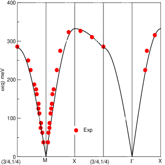
Figure 1: The theoretical spin spectra (149)-(153) (solid lines) plotted in the second Brillouin zone for $\mu^{0}=565.6$ meV and $W^{0}_{s1}=49.6$ meV and the experimental data of Ref. LCO-neutr-scatt (circles) in meV. Such theoretical magnitudes correspond to $t\approx 0.295$ eV and $U\approx 1.800$ eV, so that $U/4t\approx 1.525$. The momentum is given in units of $2\pi$. The solid lines plotted here correspond to the simple analytical expressions provided in Eqs. (149)-(153). Those plotted in Fig. 5 of Ref. LCO-Hubbard-NuMi are very similar yet are obtained within the standard formalism of many-body physics by summing up an infinite number of ladder diagrams. Experimental points from Ref. LCO-neutr-scatt .

Next let us consider the high symmetry directions in the Brillouin zone. Indeed, the curves plotted in Fig. 5 of Ref. LCO-Hubbard-NuMi refer only to such directions and the use of our above general expressions leads for $U/4t=1.525$ to an excellent agreement with such curves. These directions correspond also to those measured by high-resolution inelastic neutron scattering in LCO, as plotted in Fig. 3 (A) of Ref. LCO-neutr-scatt . We denote such symmetry directions by $MO$, $\Gamma O$, $XM$, $\Gamma X$, and $XO$. They connect the momentum-space points $M=[\pi,\pi]$, $O=[\pi/2,\pi/2]$, $\Gamma=[0,0]$, and $X=[\pi,0]$ of the general spin-wave spectrum provided in Eq. (146). The use of that equation reveals that the spin-wave excitation spectrum is in such symmetry directions given by,

$$\omega_{\Gamma O}(\vec{k}) = {\mu^{0}\over 2}\sin(k_{i})\,,$$

$$\vec{k} = [\pi,-\pi]-[\pi/2-k_{i},-\pi/2-k_{i}]-[\pi/2,-\pi/2]$$ (149)

$$= [k_{i},k_{i}]\,;\hskip 14.22636ptk_{i}=k_{x}=k_{y}\in(0,\pi/2)\,,$$

$$\omega_{MO}(\vec{k}) = {\mu^{0}\over 2}\sin(k_{i})\,,$$

$$\vec{k} = [\pi,\pi]-[\pi/2-k_{i},3\pi/2-k_{i}]-[\pi/2,-\pi/2]$$ (150)

$$= [k_{i},k_{i}]\,;\hskip 14.22636ptk_{i}=k_{x}=k_{y}\in(\pi/2,\pi)\,,$$

$$\omega_{\Gamma X}(\vec{k}) = \left[{\mu^{0}\over 2}+W^{0}_{s1}\right]\sin(k_{x}/2)\,,$$

$$\vec{k} = [\pi,-\pi]-[\pi/2-k_{x}/2,-\pi/2-k_{x}/2]$$ (151)

$$- [\pi/2-k_{x}/2,-\pi/2+k_{x}/2]$$

$$= [k_{x},0]\,;\hskip 14.22636ptk_{x}\in(0,\pi)\,,$$

$$\omega_{XM}(\vec{k}) = \left[{\mu^{0}\over 2}+W^{0}_{s1}\right]\cos(k_{y}/2)\,,$$

$$\vec{k} = [\pi,\pi]-[-k_{y}/2,\pi-k_{y}/2]-[k_{y}/2,-k_{y}/2]$$ (152)

$$= [\pi,k_{y}]\,;\hskip 14.22636ptk_{y}\in(0,\pi)\,,$$

$$\omega_{XO}(\vec{k}) = {\mu^{0}\over 2}-W^{0}_{s1}\cos(k_{x})$$

$$= {\mu^{0}\over 2}+W^{0}_{s1}\cos(k_{y})\,,$$

$$\vec{k} = [\pi,-\pi]-[0,-\pi]-[\pi-k_{x},-\pi+k_{x}]$$ (153)

$$= [\pi,\pi]-[0,\pi]-[k_{y},-k_{y}]$$

$$= [k_{x},\pi-k_{x}]\,;\hskip 7.11317ptk_{x}\in(\pi/2,\pi)$$

$$= [\pi-k_{y},k_{y}]\,;\hskip 7.11317ptk_{y}\in(0,\pi/2)\,.$$

The theoretical spin excitation spectra (149)-(153) are plotted in Fig. 1 (solid line) for $\mu^{0}=565.6$ meV and $W^{0}_{s1}=49.6$ meV together with the experimental results (circles) for $T=10$ K. This gives a Mott-Hubbard gap $2\mu^{0}=1131.2$ meV. The spin-spectrum expressions provided in Eqs. (149)-(153) refer to the first Brillouin zone. In Fig. 1 we plot them in the second Brillouin zone, alike in Fig. 3 (A) of Ref. LCO-neutr-scatt and Fig. 5 of Ref. LCO-Hubbard-NuMi . An excellent quantitative agreement is reached for these magnitudes of the involved energy scales, which according to the complementary results of Ref. LCO-Hubbard-NuMi correspond to $U/4t\approx 1.525$ and $t\approx 295$ meV. Moreover, from the use of the relation $\Delta_{0}\approx r_{s}\,4W_{s1}^{0}$ of Eq. (112) we find that $\Delta_{0}\approx 84$ meV for $U/4t\approx u_{*}=1.525$. The magnitudes of the energy scales $\Delta_{0}$, $4W^{0}_{s1}$, and $\mu^{0}/2$ found here for $U/4t\approx 1.525$ are given in Table III together with those for $U/4t\ll 1$, $U/4t=u_{0}$, and $U/4t\gg 19$. The magnitude of energy parameter $\Delta_{0}$ interpolates between that of $\mu^{0}/2$ for $U/4t\ll 1$ and $4W^{0}_{s1}$ for $U/4t\gg 1$. It reaches a maximum magnitude approximately given by $\Delta_{0}\approx t/\pi\approx 0.318\,t$ at $U/4t=u_{0}\approx 1.302$.

$U/4t$	$\Delta_{0}$	$4W^{0}_{s1}$	$\mu^{0}/2$
$\ll 1$	$16t\,e^{-\pi\sqrt{4t/U}}$	$16t$	$16t\,e^{-\pi\sqrt{4t/U}}$
$u_{0}$	$t/\pi\approx 0.318\,t$	$e^{1}t/\pi\approx 0.865\,t$	$e^{1}t/\pi\approx 0.865\,t$
$u_{*}$	$0.285\,t$	$0.673\,t$	$0.959\,t$
$\gg 19$	$\pi\,[4t]^{2}/U$	$\pi\,[4t]^{2}/U$	$[U/4-2t]$

Table 3: Approximate magnitudes of the energy scales $2\Delta_{0}$, $4W^{0}_{s1}$, and $\mu^{0}/2$ for different values of $U/4t$. The energy parameter $\Delta_{0}$ interpolates between $\mu^{0}/2\approx 16t\,e^{-\pi\sqrt{4t/U}}$ for $U/4t\ll 1$ and $4W^{0}_{s1}\approx\pi\,[4t]^{2}/U$ for $U/4t\gg 19$ and goes through a maximum magnitude ${\rm max}\,\{\Delta_{0}\}\approx t/\pi$ at the $U/4t$ value $U/4t=u_{0}\approx 1.302$ at which $\mu^{0}/2\approx 4W^{0}_{s1}$. The magnitudes of $\Delta_{0}$, $4W^{0}_{s1}$, and $\mu^{0}/2$ found here for $U/4t=u_{*}=1.525$ are also given.

For the intermediate value $U/4t\approx u_{*}=1.525\in(u_{0},u_{1})$ corresponding to Fig. 1 our investigations find the relation $W_{s1}^{0}\approx 0.168\,t$, which for a constant value of $t$ provides a $W_{s1}^{0}$ magnitude about twelve times smaller than that found by the use of the limiting expression $W^{0}_{s1}\approx J\approx 4\pi\,t^{2}/U\approx 2.060\,t$ for that $U/4t$ value. Hence for the model on the square lattice the usual energy scale $J\approx 4\pi\,t^{2}/U$ controls the physics for a smaller $U/4t$ range than in 1D, which corresponds to very large $U/4t\gg 19$ values. As discussed in Ref. companion , the value $U/4t\approx 19$ is that at which the energy scale $J\approx 4\pi\,t^{2}/U$ reads $J=0.168\,t$ and thus has the magnitude that $W_{s1}^{0}$ reaches at $U/4t\approx 1.525$. This is why the large-$U/4t$ limiting expressions $W^{0}_{s1}\approx J$ and $\Delta_{0}\approx 4J$ are valid for $U/4t\gg 19$. It follows that the intermediate-$U/4t$ range plays a major role in the physics of the square-lattice quantum liquid studied in this paper and in Refs. cuprates0 ; cuprates .

The above results are consistent with the momentum values of the $c$ and $s1$ fermions being good quantum numbers. Furthermore, they confirm that the predictions of the square-lattice quantum liquid theory concerning the spin spectrum at half filling agree both with experiments on the parent compound LCO and results obtained by the standard formalism of many-body physics.

VI.3 Relation to other schemes where the fermions emerge from individual spin-$1/2$ spins or spinons

For most previous studies on the large-$U$ Hubbard model and $t-J$ model on a square lattice involving for instance the slave particle formalism 2D-MIT ; Fazekas ; Xiao-Gang or Jordan-Wigner transformations Feng the spinless fermions arise from individual spin-$1/2$ spins or spinons. In contrast, within our $s1$ fermion extended Jordan-Wigner transformation the $s1$ fermions emerge from spin-neutral two-spinon composite $s1$ bond particles. Indeed, here the hard-core bosons refer to spin-neutral two-spinon $s1$ bond operators. Often in previous related schemes involving spin-liquid mean-field theories, which refer in general to individual spin-$1/2$ spinons or spinless fermions that emerge from them, such objects are coupled to a gauge field 2D-MIT ; Xiao-Gang . Since in 2D gauge theory is confining, in some of these liquids individual spin-$1/2$ spinons are not observable, as in for instance in the simple dimer state Xiao-Gang .

Here the original hard-core particles themselves are spin-neutral two-spinon objects. Furthermore, since the spin-$1/2$ spinons have been constructed to inherently referring here to the rotated-electron singly occupied sites, the one-rotated-electron-per-site constraint is naturally fulfilled for $U/4t>0$ so that the fluctuations needed to enforce such a constraint are for the square-lattice model incorporated in the electron - rotated-electron unitary operator $\hat{V}$. Related resonating-valence-bond pictures for spin-singlet occupancy configurations of ground states were considered long ago Fazekas ; Pauling , yet often problems arise in the construction of energy eigenstates due to bond states being overcomplete and non-orthogonal.

Motivated by previous studies where the spinless fermions arise from individual spin-$1/2$ spins or spinons, we have also performed a Jordan-Wigner transformation for the model both on the square and 1D lattices whose spinless fermions emerge from the spin-$1/2$ spinon operators $s^{\pm}_{\vec{r}_{j}}$ of Eq. (11). According to Eqs. (13) and (14) such operators have a hard-core character and the corresponding spinons are well-defined for $U/4t>0$. One then finds out that for 1D the momentum values of the emerging spinless fermions do not coincide with the quantum numbers of the exact solution. In contrast, the discrete momentum values of the $s1$ fermions emerging from spin-neutral two-spinon $s1$ bond particles correspond to such quantum numbers, as confirmed in Ref. companion .

For the model on the square lattice in the one- and two-electron subspace considered in this paper and of interest for the further investigations on real materials of Refs. cuprates0 ; cuprates , our description occupancy configurations of the $c$ fermions and $s1$ fermions generate according to the analysis of Ref. companion energy eigenstates. This is in contrast to the alternative scheme in terms of spinless fermions emerging from the spin-$1/2$ spinon operators $s^{\pm}_{\vec{r}_{j}}$ of Eq. (11), which generates a complete set of states in that subspace, which however are not in general energy eigenstates. The same applies to the 1D model in the whole Hilbert space. Following the results of Ref. companion , the momentum values of the $c$ and $s1$ fermions are good quantum numbers for the model on the square lattice in the one- and two-electron subspace. Our scheme uses several approximations to access the shape of the $s1$ boundary line, and the $c$ and $s1$ fermion energy dispersions. Our corresponding results are not exact, yet they rely on a general subspace structure and correct symmetries, which are compatible with the unknown exact expressions of the quantities under consideration. We expect that our approximations provide a good description of the physics for intermediate values of $U/4t$, consistently with the results of the previous subsection concerning the half-filling spin spectrum. That spin spectrum is found above to lead for the model on the square lattice to analytical expressions for the spin-wave spectrum that agree with the corresponding numerical curves obtained by a different controlled approximation involving the sum of an infinite set of electronic ladder diagrams LCO-Hubbard-NuMi .

For the model on the square lattice the above alternative scheme leads to a vector potential of the same general form as that given in Eq. (24), but with the operator $n_{\vec{r}_{j},s1}$ of Eq. (23) replaced by $[1/2+s^{x_{3}}_{\vec{r}_{j}}]$ and the real-space variable $\vec{r}_{j}$ referring to the spin effective lattice rather than to the $s1$ effective lattice. Except that such a scheme refers here to the spins of the rotated electrons that singly occupy sites and is valid for $U/4t>0$, it is identical to the spin problem and corresponding Jordan-Wigner transformation considered in Ref. Wang .

A qualitative difference, which has impact on the physics, is that a $x\geq 0$ and $m=0$ ground state is described here by a full $s1$ momentum band whereas for the spinless fermions emerging from the spin-$1/2$ spinon operators $s^{\pm}_{\vec{r}_{j}}$ of Eq. (11) it is described by a half-filled spin band. This is alike the Wigner-Jordan (WJ) fermions associated with the WJ representation of quantum spins with antiferromagnetic interaction of Ref. Wang , which at zero temperature fill exactly half of the total states. In turn, within our $c$ and $s1$ fermion description the $s1$ momentum band is full for the initial $x\geq 0$ and $m=0$ ground state and addition or removal of one electron leads to the emergence of a single $s1$ fermion hole in that band. Indeed, following the transformation laws under the electron - rotated-electron unitary transformation of the objects whose occupancy configurations generate the energy eigenstates of the square-lattice model in the one- and two-electron subspace, excited states with three or a larger odd number of $s1$ fermion holes have nearly no overlap with one-electron excitations companion . Furthermore, symmetry selection rules companion impose that such an overlap vanishes exactly for excited states with an even number of $s1$ fermion holes.

The emergence of a single hole in the $s1$ band upon creation or annihilation of one electron plays a major role in the strong phase-space, exclusion-principle, and energy and momentum conservation restrictions of the $s1$ - $s1$ fermion and $s1$ - $c$ fermion scattering. Within the emergence of a single $s1$ fermion hole there are obviously no available final channels associated with $s1$ - $s1$ fermion scattering. The above restrictions, together with the isotropic and anisotropic character of the $c$ Fermi line and $s1$ boundary line, respectively, leads for $x>0$ to unusual one-electron scattering properties cuprates . This includes an anisotropic one-electron inverse lifetime and scattering rate linear in the excitation energy $\omega$, in excellent quantitative agreement with that observed in recent angle-resolved photoemission studies of the optimally doped high-temperature superconductor LSCO Kam ; PSI-ANI-07 . Such an inverse lifetime is different from that characteristic of an isotropic conventional 2D electron liquid, which is proportional to $(\omega/E_{F})^{2}\ln(E_{F}/\omega)$ where $E_{F}$ denotes the Fermi energy 2D-1/tau-1 .

In turn, for the spinless fermions emerging from the spin-$1/2$ spinon operators $s^{\pm}_{\vec{r}_{j}}$ given in Eq. (11), that their momentum band is half filled implies that the ground-state configurations contain as many spinless fermions as spinless fermion holes. It follows that in contrast to the $s1$ fermions, upon one-electron excitations there are available final channels for both spinless fermion - spinless fermion and spinless fermion - $c$ fermion inelastic collisions. In addition, since the momenta carried by such spinless fermions are not good quantum numbers, their interactions are not residual so that in contrast to the $c$ and $s1$ fermion description one cannot use Fermi’s golden rule in terms of a collision integral as that associated with the $c$ - $s1$ fermion interactions to calculate the one-electron lifetime cuprates0 . In principle the final expressions should be the same independently of the representation. However, the one-electron scattering problem is much more complex when expressed in terms of the interactions of the spinless fermions emerging from the spin-$1/2$ spinon operators $s^{\pm}_{\vec{r}_{j}}$ and so far we could not solve it.

Finally, only within our description do the $s1$ fermion occupancy configurations that generate the spin degrees of freedom of $x>0$ and $m=0$ ground states of the 1D model become in the $U/4t\rightarrow\infty$ limit those of the spins of the well-known spin-charge factorized wave function introduced independently by Woynarovich Woy and by Ogata and Shiba Ogata , respectively. Moreover, only within that description become such ground-state configurations of the model on a square lattice in the $U/4t\rightarrow\infty$ limit and within the suitable mean-field approximation (29) for the fictitious magnetic field ${\vec{B}}_{s1}$ of Eq. (21) those of a $\nu_{s1}=1$ full lowest Landau level with $N_{a_{s1}}^{2}=N/2$ one-$s1$-fermion degenerate states of the 2D QHE.

VII Concluding remarks

The operator description introduced in Ref. companion for the Hubbard model on the square lattice in the one- and two-electron subspace as defined in that rteference has been constructed to inherently the discrete momentum values of the $c$ and $s1$ fermions beeing good quantum numbers. Complementarily, in this paper we derive approximate results and expressions for the $s1$ band boundary line, $c$ and $s1$ fermion energy dispersions, and corresponding $c$ and $s1$ fermion velocities of the square-lattice quantum liquid introduced in that reference.

That the $s1$ band remains full alike for for $x>0$ and $m=0$ ground states alike for $x=0$ is related to the degree of localization in real space of the $s1$ fermion holes, which upon one- and two-electron excitations emerge near the $s1$ boundary line at momenta pointing in or near the anti-nodal directions. Indeed, the $s1$ fermion velocity studied in Section V vanishes for $s1$ boundary-line momenta pointing in such directions. The corresponding finite-energy real-space excitations occur near the pseudogap energy and break translational symmetry locally, due to the square $s1$ effective lattice spacing being given by $a_{s1}=\sqrt{2/(1-x)}\,a$ rather than by the original square-lattice spacing $a$. In turn, for $x>0$ the $c$ band has for the ground state an isotropic $c$ Fermi line associated with a finite $c$ fermion velocity so that the low-energy one- and two-electron excitations involving creation of $c$ fermions or $c$ fermion holes near the $c$ Fermi line and $s1$ fermion holes with momenta pointing in and near the nodal directions have a delocalized character. Consistently, in contrast to the isotropic $c$ Fermi line it is found in this paper that the $s1$ boundary line is rather anisotropic, the corresponding $s1$ fermion velocity vanishing and reaching its maximum magnitude for momenta pointing in the anti-nodal and nodal directions, respectively.

Such properties of the $c$ Fermi line and $s1$ boundary line are behind the anisotropy of the Fermi velocity, which is larger for smaller $x$. They remain valid for the square-lattice quantum liquid weakly perturbed by the effects of 3D anisotropy investigated in Refs. cuprates0 ; cuprates . The results of that reference are fully consistent with the two-gap scenario observed in the hole-doped cuprates superconductors two-gaps ; k-r-spaces . For instance, there is a direct connection to the recent experimental studies of Ref. k-r-spaces . Indeed, the excitations involving coherent virtual-electron pairs whose spinless charge-$-2e$ zero-momentum $c$ fermion pairs are assisted by spin-singlet two-spinon composite $s1$ fermions of momenta pointing in or near the nodal directions correspond to the superconducting superfluid of delocalized Cooper pairs in momentum space observed in such experiments. In turn, the finite-energy excitations involving $s1$ fermions whose momenta point in and near the anti-nodal directions refer to the locally translational-breaking pseudogap states in real space observed in the same experiments.

Furthermore, the investigations of Refs. cuprates0 ; cuprates provide evidence that accounting for the interplay of the electronic correlations described by the square-lattice quantum liquid of $c$ and $s1$ fermions studied in this paper with the weak effects of 3D anisotropy and intrinsic disorder leads to a successful theoretical description of the unusual properties of the hole-doped cuprates. Indeed, the corresponding scheme introduced in Ref. cuprates , leads to quantitative agreement with the universal properties of the hole-doped cuprates with superconducting zero-temperature critical hole concentrations $x_{c}\approx 0.05$ and $x_{*}\approx 0.27$. For instance, the isotropic character of the $c$ Fermi line and the anisotropy of the $s1$ boundary line found in this paper combined with the $s1$ band being full and having a single hole for $x>0$ and $m=0$ ground states and their one-electron excited states, respectively, leads to unusual one-electron scattering properties controlled by the $c$ - $s1$ fermion inelastic collisions. The investigations of that reference profit from such a $c$ and $s1$ fermion description of the one-electron scattering problem and find a strongly anisotropic one-electron inverse lifetime and scattering rate in excellent quantitative agreement with that observed in recent angle-resolved photoemission studies of the optimally doped high-temperature superconductor LSCO Kam ; PSI-ANI-07 . The studies of Ref. cuprates also successfully address the normal-state linear-$T$ resistivity in that and other hole doped cuprates LSCO-resistivity ; Y-resistivity , neutron resonance mode observed in families of hole doped cuprates with critical temperature $T_{c}\approx 95$ K two-gaps , hole-concentration $x$ dependence of several physical quantities such as $T_{c}$ and the superfluid density, and the LSCO neutron-scattering low-energy incommensurate peaks 2D-MIT ; pseudogap-review .

In conclusion, the results of Refs. cuprates0 ; cuprates confirm that addition to the square-lattice quantum liquid of $c$ and $s1$ fermions studied in this paper of small 3D anisotropy and intrinsic disorder effects leads to a successful description of the unusual properties observed in the hole-doped cuprates.

Appendix A The one- and two-electron subspace

The square-lattice quantum liquid of $c$ and $s1$ fermions studied in this paper refers to the one- and two-electron subspace of the Hubbard model on the square lattice as defined in Ref. companion . Here we provide some basic information about such a subspace needed for the studies of this paper. The results summarized in the following are derived and discussed in that paper and in Ref. s1-bonds .

For hole concentrations $0\leq x\leq 1$ and subspaces spanned by energy eigenstates with constant eigenvalue $S_{c}$ of the generator of the global $U(1)$ symmetry of Ref. bipartite there is a vacuum $|0_{\eta s}\rangle$, which remains invariant under the electron - rotated-electron unitary transformation. For $x=1$ such a vacuum coincides with the electronic vacuum whereas for $0\leq x<1$ it refers to the $m=(1-x)$ fully polarized ground state. For the 1D model one can derive a closed form analytical expression for the critical magnetic field $H_{c}$ for fully polarized ferromagnetism as function of the electronic density $n=(1-x)$ and $u=U/4t$. It is given in Eq. (2) of Ref. renor and plotted in Fig. 1 of that reference. Alike in 1D, it is expected that for the model on the square lattice the magnitude $H_{c}$ of the in-plane critical field for fully polarized ferromagnetism is for all values of $U/4t$ a decreasing function of the hole concentration $x$, which vanishes for $x\rightarrow 1$. It is expected as well that for $x<1$ it is a decreasing function of $U/4t$, which vanishes for $U/4t\rightarrow\infty$. Such a vacuum reads,

$$|0_{\eta s}\rangle=|0_{\eta};N_{a_{\eta}}^{D}\rangle\times|0_{s};N_{a_{s}}^{D}\rangle\times|GS_{c};2S_{c}\rangle\,,$$ (154)

where the $\eta$-spin $SU(2)$ vacuum $|0_{\eta};N_{a_{\eta}}^{D}\rangle$ associated with $N_{a_{\eta}}^{D}$ independent $+1/2$ $\eta$-spinons, the spin $SU(2)$ vacuum $|0_{s};N_{a_{s}}^{D}\rangle$ with $N_{a_{s}}^{D}$ independent $+1/2$ spinons, and the $c$ $U(1)$ vacuum $|GS_{c};2S_{c}\rangle$ with $N_{c}=2S_{c}$ $c$ fermions remain invariant under the electron - rotated-electron unitary transformation. For such a fully polarized problem the on-site electronic repulsion has no effects so that for $m\rightarrow(1-x)$ and $H\rightarrow H_{c}$ the rotated electrons become electrons. In that limit the $N_{c}=2S_{c}=N$ $c$ fermions are the non-interacting spinless fermions, which describe the charge degrees of freedom of the $N$ electrons. The $c$ $U(1)$ vacuum $|GS_{c};2S_{c}\rangle$ can be written as,

$$|GS_{c};2S_{c}\rangle=\prod_{j=1}^{2S_{c}}f^{{\dagger}}_{{\vec{q}}_{j},c}|GS_{c};0\rangle\,.$$ (155)

Here $|GS_{c};0\rangle$ refers to the $x=1$ and $N=0$ electronic vacuum,

$$|0_{elec}\rangle=|0_{\eta};N_{a}^{D}\rangle\times|0_{s};0\rangle\times|GS_{c};0\rangle\,.$$ (156)

The state (155) is a particular case of the state of the same form appearing in Eq. (32). In turn, the vacuum (156) corresponds to a limiting case of the vacuum (154) associated with the values $N_{a_{\eta}}^{D}=N_{a}^{D}$, $N_{a_{s}}^{D}=0$, and $2S_{c}=0$.

The $c$ fermion, $\alpha\nu$ fermion, and independent $\eta$-spinon and independent spinon description of Ref. companion refers to a complete set of $4^{N_{a}^{D}}$ momentum eigenstates $|\Phi_{U/4t}\rangle={\hat{V}}^{{\dagger}}|\Phi_{\infty}\rangle$ generated from application onto the corresponding $U/4t\rightarrow\infty$ states $|\Phi_{\infty}\rangle$ of the electron - rotated-electron unitary operator ${\hat{V}}^{{\dagger}}$. Such states can be generated from their LWS as,

$$|\Phi_{U/4t}\rangle=\prod_{\alpha=\eta,\,s}\frac{({\hat{S}}^{{\dagger}}_{\alpha})^{L_{\alpha,\,-1/2}}}{\sqrt{{\cal{C}}_{\alpha}}}|\Phi_{LWS;U/4t}\rangle\,;\hskip 9.95863pt{\cal{C}}_{\alpha}=\delta_{L_{\alpha,\,-1/2},\,0}+\prod_{l=1}^{L_{\alpha,\,-1/2}}l\,[\,L_{\alpha}+1-l\,]\,,$$ (157)

where $L_{\alpha,\,-1/2}$ is the number of $\eta$-spin-projection $-1/2$ independent $\eta$-spinons $(\alpha=\eta$) or spin-projection $-1/2$ independent spinons $(\alpha=s$). The corresponding LWS $|\Phi_{LWS;U/4t}\rangle={\hat{V}}^{{\dagger}}|\Phi_{LWS;\infty}\rangle$ and $U/4t\rightarrow\infty$ LWS belonging to the same $V$ tower read,

$$|\Phi_{LWS;U/4t}\rangle=[\prod_{\alpha}\prod_{\nu}\prod_{{\vec{q}}\,^{\prime}}f^{{\dagger}}_{{\vec{q}}\,^{\prime},\alpha\nu}|0_{\alpha};N_{a_{\alpha}^{D}}\rangle][\prod_{{\vec{q}}}f^{{\dagger}}_{{\vec{q}},c}|GS_{c};0\rangle]\,;\hskip 7.11317ptf^{{\dagger}}_{{\vec{q}}\,^{\prime},\alpha\nu}={\hat{V}}^{{\dagger}}\,{\mathcal{F}}^{{\dagger}}_{{\vec{q}}\,^{\prime},\alpha\nu}\,{\hat{V}}\,;\hskip 7.11317ptf^{{\dagger}}_{{\vec{q}},c}={\hat{V}}^{{\dagger}}\,{\mathcal{F}}^{{\dagger}}_{{\vec{q}},c}\,{\hat{V}}\,,$$ (158)

and

$$|\Phi_{LWS;\infty}\rangle=[\prod_{\alpha}\prod_{\nu}\prod_{{\vec{q}}\,^{\prime}}{\mathcal{F}}^{{\dagger}}_{{\vec{q}}\,^{\prime},\alpha\nu}|0_{\alpha};N_{a_{\alpha}^{D}}\rangle][\prod_{{\vec{q}}}{\mathcal{F}}^{{\dagger}}_{{\vec{q}},c}|GS_{c};0\rangle]\,,$$ (159)

respectively. Here ${\mathcal{F}}^{{\dagger}}_{{\vec{q}},c}$ and ${\mathcal{F}}^{{\dagger}}_{{\vec{q}}\,^{\prime},\alpha\nu}$ are the $c$ fermion and $\alpha\nu$ fermion creation operators for $U/4t\rightarrow\infty$, respectively.

For the 1D Hubbard model the states (157) and (158) are both energy and momentum eigenstates. In turn, since for the model on the square lattice the set of $\alpha\nu$ translation generators ${\hat{\vec{q}}}_{\alpha\nu}$ in the presence of the fictitious magnetic fields ${\vec{B}}_{\alpha\nu}$ considered in Ref. companion whose eigenvalues are the components of the $\alpha\nu$ band momenta do not in general commute with the Hamiltonian and the corresponding set of $\alpha\nu$ fermion numbers $\{N_{\alpha\nu}\}$ are not in general conserved, such states are not energy eigenstates and the microscopic momenta carried by the $\alpha\nu$ fermions are not in general good quantum numbers. However, such states have been constructed to inherently being $S_{\eta}$, $S_{\eta}^{z}$, $S_{s}$, $S_{s}^{z}$, $S_{c}$, and momentum eigenstates and each energy eigenstate $|\Psi_{U/4t}\rangle={\hat{V}}^{{\dagger}}|\Psi_{\infty}\rangle$ can be expressed as a suitable superposition of a well-defined set of $|\Phi_{U/4t}\rangle={\hat{V}}^{{\dagger}}|\Phi_{\infty}\rangle$ momentum eigenstates (157) with the same momentum eigenvalue and values of $S_{\eta}$, $S_{\eta}^{z}$, $S_{s}$, $S_{s}^{z}$, $S_{c}$, $C_{\eta}=\sum_{\nu}\nu\,N_{\eta\nu}$, and $C_{s}=\sum_{\nu}\nu\,N_{s\nu}$ and the same $c$ fermion momentum distribution function $N_{c}({\vec{q}})$ companion . As discussed in this paper, for the model on the square lattice in the one- and two-electron subspace the form of the states (157) and (158) simplifies to that provided in Eq. (32) and as justified in Ref. companion such states are energy eigenstates so that the microscopic momenta carried by the $c$ and $s1$ fermions are good quantum numbers

For spin densities $m=0$ and $m=(1-x)$ and $U/4t\rightarrow\infty$ and $U/4t\geq 0$, respectively, the $c$ fermions are for $0<x<1$ non-interacting and for the model on the square lattice have an energy dispersion given by,

$$\epsilon^{0}_{c}(\vec{q})=-2t\,[\cos(q_{x_{1}})+\cos(q_{x_{2}})-\cos(k_{Fx_{1}})-\cos(k_{Fx_{2}})]\,.$$ (160)

Here $k_{Fx_{1}}$ and $k_{Fx_{2}}$ are the Cartesian coordinates of the Fermi momentum $\vec{k}_{F}$,

$$\vec{k}_{F}=k_{F}(\phi)\,{\vec{e}}_{\phi}\,;\,;\hskip 14.22636pt\phi=\arctan\left({k_{Fx_{2}}\over k_{Fx_{1}}}\right)\,;\hskip 9.95863pt\phi\in(0,2\pi)\,.$$ (161)

For such values of $m$ and $U/4t$ the corresponding Fermi line encloses a momentum area,

$$\int_{0}^{2\pi}{d\phi\over 2\pi}\,\pi\left[k_{F}(\phi)\right]^{2}=(1+x)\,4\pi^{2}\,.$$ (162)

It is twice the area enclosed by the Fermi line at $m=0$ and $U/4t=0$.

Two energy scales that play a key role in the square-lattice quantum liquid are the chemical potential $\mu$ and the maximum $s1$ fermion spinon-pairing energy $2|\Delta|$ of Eq. (114), which in the limit $x\rightarrow 0$ equals the energy scale $2\Delta_{0}$ whose magnitudes are provided in Table III. Within the LWS representation, the convention that $\mu$ has the same sign as the hole concentration $x$ is used. For $0<x<1$ and $m=0$ the chemical potential is an increasing function of the hole concentration $x$ whose values belong to the range,

$$\mu^{0}\leq\mu(x)\leq\mu^{1}\,;\hskip 14.22636pt0<x<1\,,\hskip 9.95863ptm=0\,,$$ (163)

where $\mu^{1}\equiv\lim_{x\rightarrow 1}\mu$. $\mu^{1}$ reads,

$$\mu^{1}=[U/2+2Dt]\,;\hskip 14.22636ptD=1,2\,.$$ (164)

Moreover, $\mu^{0}$ has the following approximate limiting behaviors companion ,

$$\mu^{0}\approx{U\over 2\pi^{2}}\left({[8\pi]^{2}t\over U}\right)^{D/2}e^{-2\pi\left({t\over U}\right)^{1/D}}\,,\hskip 7.11317ptU/4t\ll 1\,;\hskip 14.22636pt\mu^{0}\approx[U/2-2Dt]\,,\hskip 7.11317ptU/4t\gg 1\,,\hskip 7.11317ptD=1,2\,,$$ (165)

so that $\mu^{0}\rightarrow 0$ as $U/4t\rightarrow 0$ whereas $\mu^{0}\rightarrow\infty$ for $U/4t\gg 1$ for both the model on the 1D and square lattices. As discussed in previous sections, $2\mu^{0}$ is the half-filling Mott-Hubbard gap.

Another energy scale that plays an important role is the energy $\epsilon_{c}$ for addition onto a $x\geq 0$ and $m=0$ ground state of one $c$ fermion and the corresponding energy energy $-\epsilon_{c}$ for removal from that state of one $c$ fermion, which obey the inequalities,

$$0\leq\epsilon_{c}\leq[4Dt-W^{p}_{c}]\,;\hskip 14.22636pt0\leq-\epsilon_{c}\leq W^{p}_{c}\,;\hskip 14.22636ptD=1,2\,,$$ (166)

respectively. In turn, the energy $-\epsilon_{s1}$ for addition to a $x\geq 0$ and $m=0$ ground state of one $s1$ fermion hole obeys the inequality,

$$0\leq-\epsilon_{s1}\leq{\rm max}\,\{W_{s1},(D-1)|\Delta|\}\,,\hskip 9.95863ptD=1,2\,.$$ (167)

In such inequalities $W^{p}_{c}$ and $W^{h}_{c}=[4Dt-W^{p}_{c}]$ are the ground-state $c$ fermion and $c$ fermion-hole energy-dispersion bandwidths, respectively, $W^{h}_{c}=[4Dt-W^{p}_{c}]\in(0,4Dt)$ increases monotonously upon increasing the hole concentration within the range $x\in(0,1)$, $W_{s1}$ is the $s1$ fermion auxiliary energy-dispersion bandwidth of Eq. (114), and the energy parameter $|\Delta|$ corresponds for the model on the square lattice to the maximum $s1$ fermion pairing energy per spinon of Eq. (117). The energy $W_{s1}^{0}=\lim_{x\rightarrow 0}W_{s1}$ has the following approximate limiting behaviors companion ,

$$W_{s1}^{0} = 2Dt\,;\hskip 14.22636ptU/4t=0\,,$$ (168)

$$\approx 2D\pi\,t^{2}/U\,;\hskip 14.22636ptU/4t\gg 1\,.$$

For the model on the square lattice the large-$U/4t$ expression is expected to be a good approximation for very large values $U/4t\gg 19$, as justified in this paper and Ref. companion .

The one- and two-electron subspace is spanned by a given initial $x\geq 0$ and $m=0$ ground state and a well-defined set of its excited energy eigenstates of excitation energy $\omega<2\mu$ for $x>0$ and $\omega<\mu^{0}$ for $x=0$. Such states have no $-1/2$ $\eta$-spinons, $2\nu$-$\eta$-spinon composite $\eta\nu$ fermions, and $2\nu^{\prime}$-spinon composite $s\nu^{\prime}$ fermions with $\nu^{\prime}\geq 3$ spinon pairs so that $N_{\eta\nu}=0$ and $N_{s\nu^{\prime}}=0$ for $\nu^{\prime}>1$, whereas according to the studies of Ref. companion the numbers of independent $\pm 1/2$ spinons and that of $s2$ fermions are restricted to the following ranges,

$$L_{s,\,\pm 1/2}=0,1\,;\hskip 14.22636ptN_{s2}=0\,,\hskip 9.95863pt{\cal{N}}=1\,;\hskip 14.22636pt2S_{s}+2N_{s2}=0,1,2\,,\hskip 9.95863pt{\cal{N}}=2\,.$$ (169)

Here ${\cal{N}}=1,2$ refers to the ${\cal{N}}$-electron operators whose application onto the ground state leads to the excited states under consideration. Furthermore, the numbers of $c$ and $s1$ fermions read $N_{c}=N=(1-x)\,N_{a}^{D}$ and $N_{s1}=[N/2-2N_{s2}-S_{s}]=(1-x)\,N_{a}^{D}/2-[2N_{s2}+S_{s}]$, respectively.

From analysis of the ground-state occupancies found in Ref. companion , for the one- and two-electron subspace there occur the fourteen classes of elementary excited states relative to an initial $x\geq 0$ and $m=0$ ground state whose numbers and number deviations are given in Table 4. The table provides the values of the deviations $\delta N_{c}^{h}$ and numbers $N_{s1}^{h}$ of such excited states, corresponding electron number deviations $\delta N_{\uparrow}$ and $\delta N_{\downarrow}$, and independent-spinon numbers $L_{s,\,+1/2}$ and $L_{s,\,-1/2}$ and $s2$ fermion numbers $N_{s2}$ restricted to the value ranges of that subspace. The spin $S_{s}$ and deviations $\delta S_{c}$, $\delta N_{s1}=[\delta S_{c}-S_{s}-2N_{s2}]$, and $\delta N_{a_{s1}}=[\delta S_{c}+S_{s}]$ of each excitation are also given.

In reference companion it is found from analysis of the transformation laws under the electron - rotated-electron unitary transformation of the objects whose occupancy configurations generate the energy eigenstates of the Hubbard model that nearly the whole one- and two-electron spectral weight is contained in the one- and two-electron subspace whose numbers are given in Table IV. If in addition we restrict our considerations to the LWS-subspace of the one- and two-electron subspace, then $L_{s,\,-1/2}=0$ in Eq. (169), whereas the values $L_{s,\,+1/2}=0,1$ for $N_{s2}=0$ and ${\cal{N}}=1$ remain valid and in $2S_{s}+2N_{s2}=0,1,2$ one has that $2S_{s}=L_{s,\,+1/2}$ for ${\cal{N}}=2$ in that equation.

For the one- and two-electron subspace of the Hamiltonian (1) only the $c$ fermions and $s1$ fermions play an active role. The numbers $N_{a}^{D}$ and $N_{a_{s1}}^{D}$ of sites of the $c$ and $s1$ effective lattices, respectively, equal the number of corresponding $c$ and $s1$ band discrete momentum values. The number $N_{a_{s1}}^{D}$, that of $s1$ fermions $N_{s1}$, and that of both unoccupied sites of the $s1$ effective lattice and $s1$ band holes $N^{h}_{s1}$ are for the one- and two-electron subspace given by,

$$N_{a_{s1}}^{D} = N_{s1}+N^{h}_{s1}=N_{a_{s}}^{D}/2+S_{s}=S_{c}+S_{s}\,;\hskip 14.22636ptN_{a_{s}}^{D}=(1-x)\,N_{a}^{D}\,,$$

$$N_{s1} = N_{a_{s}}^{D}/2-S_{s}+2N_{s2}=S_{c}-S_{s}-2N_{s2}\,;\hskip 14.22636ptN^{h}_{s1}=2S_{s}+2N_{s2}=0,1,2\,,$$ (170)

respectively, where $N_{a_{s}}^{D}=(1-x)N_{a}^{D}$ is the number of sites of the related spin effective lattice.

numbers	charge	+1$\uparrow$el.	-1$\downarrow$el.	+1$\downarrow$el.	-1$\uparrow$el.	singl.spin	tripl.spin	tripl.spin	tripl.spin	$\pm$2$\uparrow\downarrow$el.	+2$\uparrow$el.	-2$\downarrow$el.	+2$\downarrow$el.	-2$\uparrow$el.
$\delta N_{c}^{h}$	$0$	$-1$	$1$	$-1$	$1$	$0$	$0$	$0$	$0$	$\mp 2$	$-2$	$2$	$-2$	$2$
$N_{s1}^{h}$	$0$	$1$	$1$	$1$	$1$	$2$	$2$	$2$	$2$	$0$	$2$	$2$	$2$	$2$
$\delta N_{\uparrow}$	$0$	$1$	$0$	$0$	$-1$	$0$	$1$	$-1$	$0$	$\pm 1$	$2$	$0$	$0$	$-2$
$\delta N_{\downarrow}$	$0$	$0$	$-1$	$1$	$0$	$0$	$-1$	$1$	$0$	$\pm 1$	$0$	$-2$	$2$	$0$
$L_{s,\,+1/2}$	$0$	$1$	$1$	$0$	$0$	$0$	$2$	$0$	$1$	$0$	$2$	$2$	$0$	$0$
$L_{s,\,-1/2}$	$0$	$0$	$0$	$1$	$1$	$0$	$0$	$2$	$1$	$0$	$0$	$0$	$2$	$2$
$N_{s2}$	$0$	$0$	$0$	$0$	$0$	$1$	$0$	$0$	$0$	$0$	$0$	$0$	$0$	$0$
$S_{s}$	$0$	$1/2$	$1/2$	$1/2$	$1/2$	$0$	$1$	$1$	$1$	$0$	$1$	$1$	$1$	$1$
$\delta S_{c}$	$0$	$1/2$	$-1/2$	$1/2$	$-1/2$	$0$	$0$	$0$	$0$	$\pm 1$	$1$	$-1$	$1$	$-1$
$\delta N_{s1}$	$0$	$0$	$-1$	$0$	$-1$	$-2$	$-1$	$-1$	$-1$	$\pm 1$	$0$	$-2$	$0$	$-2$
$\delta N_{a_{s1}}$	$0$	$1$	$0$	$1$	$0$	$0$	$1$	$1$	$1$	$\pm 1$	$2$	$0$	$2$	$0$

Table 4: The deviations $\delta N_{c}^{h}=-2\delta S_{c}$ and numbers $N_{s1}^{h}=[2S_{s}+2N_{s2}]$ for the fourteen classes of one- and two-electron excited states of the $x>0$ and $m=0$ ground state that span the one- and two-electron subspace as defined in Ref. companion , corresponding electron number deviations $\delta N_{\uparrow}$ and $\delta N_{\downarrow}$, and independent-spinon numbers $L_{s,\,+1/2}$ and $L_{s,\,-1/2}$ and $s2$ fermion numbers $N_{s2}$ restricted to value ranges of that subspace. The spin $S_{s}$ and deviations $\delta S_{c}$, $\delta N_{s1}=[\delta S_{c}-S_{s}-2N_{s2}]$, and $\delta N_{a_{s1}}=[\delta S_{c}+S_{s}]$ of each excitation are also provided.

It is found in Ref. s1-bonds that for the one- and two-electron subspace and $N_{a}^{D}\gg 1$, the operators $g_{{\vec{r}}_{j},s1}$ (and $g^{{\dagger}}_{{\vec{r}}_{j},s1}$) related to the annihilation and creation of local $s1$ fermion operators through Eq. (16), which annihilate (and create) a $s1$ bond particle at a site of the $s1$ effective lattice of real-space coordinate ${\vec{r}}_{j}$, have the following general form both for the model on the $1D$ and square lattices,

$$g_{\vec{r}_{j},s1}=\sum_{g=0}^{N_{s1}/2D-1}h_{g}\,a_{\vec{r}_{j},s1,g}\,;\hskip 9.95863ptg_{\vec{r}_{j},s1}^{{\dagger}}=\left(g_{{\vec{r}}_{j},s1}\right)^{{\dagger}}\,;\hskip 14.22636pta_{\vec{r}_{j},s1,g}=\sum_{d=1}^{D}\sum_{l=\pm 1}\,b_{\vec{r}_{j}+{\vec{r}_{d,l}}^{\,0},s1,d,l,g}\,.$$ (171)

Hence the expression of the operator $g_{\vec{r}_{j},s1}^{{\dagger}}$ involves the operators,

$$a_{\vec{r}_{j},s1,g}^{{\dagger}}=\left(a_{{\vec{r}}_{j},s1,g}\right)^{{\dagger}}\,;\hskip 14.22636ptb_{\vec{r},s1,d,l,g}^{{\dagger}}=\left(b_{\vec{r},s1,d,l,g}\right)^{{\dagger}}\,.$$ (172)

The operators $a_{\vec{r}_{j},s1,g}^{{\dagger}}$ and $a_{\vec{r}_{j},s1,g}$ create and annihilate, respectively, a superposition of $2D=2,4$ two-site bonds of the type studied in Ref. s1-bonds and $b_{\vec{r},s1,d,l,g}^{{\dagger}}$ and $b_{\vec{r},s1,d,l,g}$ are two-site one-bond operators whose expression is given in that reference.

Appendix B Confirmation of the gauge structure of the underlying $s1$ effective lattice

The $s1$ bond-particle description of Ref. s1-bonds involves a change of gauge structure s1-bonds ; Xiao-Gang so that the real-space coordinates of the sites of the $s1$ effective lattice correspond to one of the two sub-lattices of the square spin effective lattice. Here it is confirmed that for the limit $N_{a}^{D}\gg 1$ that the description used in our studies refers to and for hole concentrations $x$ such that the density $n=(1-x)$ is finite the two choices of $s1$ effective lattice lead to the same description.

The initial ground states of the one- and two-electron subspace are $x\geq 0$, $m=0$, and $N_{s1}^{h}=0$ states. Here $N_{s1}^{h}=[N_{a_{s1}}^{D}-N_{s1}]$ is the number of unoccupied sites of the $s1$ effective lattice. Its expression is for the one- and two-electron subspace given in Eq. (170) of Appendix A along with that of the number $N_{s1}$ of $s1$ fermions. We emphasize that for the present limit $N_{a_{s1}}^{D}\gg 1$ the transformation of Eq. (25) leads precisely to the same operators $f_{\vec{q}_{j},s1}^{{\dagger}}$ and $f_{\vec{q}_{j},s1}$ independently on whether the real-space coordinates $\vec{r}_{j^{\prime}}$ of the corresponding operators $f_{\vec{r}_{j^{\prime}},s1}^{{\dagger}}$ and $f_{\vec{r}_{j^{\prime}},s1}$, respectively, are those of any of the two sub-lattices of the spin effective lattice. Indeed, the two choices of real-space variables of the $s1$ effective lattice considered in Ref. s1-bonds are for $N_{s1}^{h}=0$ states related both by the transformations $\vec{r}_{j^{\prime}}\rightarrow\vec{r}_{j^{\prime}}+a_{s1}\,{\vec{e}}_{x_{1}}$ and $\vec{r}_{j^{\prime}}\rightarrow\vec{r}_{j^{\prime}}+a_{s1}\,{\vec{e}}_{x_{2}}$. If in the expressions of Eq. (25) we replace $\vec{r}_{j^{\prime}}$ by $\vec{r}_{j^{\prime}}+a_{s1}\,{\vec{e}}_{x_{1}}$ or $\vec{r}_{j^{\prime}}+a_{s1}\,{\vec{e}}_{x_{2}}$ and transform the summations in integrals, for the periodic boundary conditions considered in Ref. s1-bonds we obtain within the limit $N_{a_{s1}}^{D}\rightarrow\infty$ exactly the same operators $f_{\vec{q}_{j},s1}^{{\dagger}}$ and $f_{\vec{q}_{j},s1}$.

This confirms that the change of gauge structure s1-bonds ; Xiao-Gang used in the construction of the $s1$ effective lattice, which consists in choosing one of the two sub-lattices of the square spin effective lattice to play the role of $s1$ effective lattice, does not affect the momentum values of the $s1$ fermions: One reaches the same momentum values and thus the same physics for the two possible choices of $s1$ effective-lattice real-space coordinates.

That change of gauge structure was made in Ref. s1-bonds for the $N_{s1}^{h}=0$ configuration state that generates the spin degrees of freedom of the $x\geq 0$ and $m=0$ ground states. As discussed in that paper, all $N_{s1}^{h}$-finite configuration states associated with the excited states generated by application of one- and two-electron operators onto such ground states can be straightforwardly constructed from the $N_{s1}^{h}=0$ configuration state. The point is that the momentum $s1$ fermion operators obtained from the transformation of Eq. (25) are precisely the same for any finite number $N_{s1}^{h}$ of $s1$ band holes, independently on whether the corresponding $N_{s1}^{h}$-finite configuration states are generated from the $N_{s1}^{h}=0$ configuration state when described by occupancy of one or the other sublattice sites. This confirms that for the limit $N_{a_{s1}}^{D}\gg 1$ the two alternative choices of real-space coordinates of the $s1$ effective lattice refer indeed to a gauge structure, as stated in Ref. Xiao-Gang .

That such a change of gauge structure leads to the same $s1$ fermions independently of the choice of the real-space coordinates of the $s1$ effective lattice is a result that applies both to the model on the square and 1D lattices.

Appendix C The $x$ dependence of the elementary function $e_{s1}(q)$ for $0<x\ll 1$ and $U/4t\geq u_{0}$

The goal of this Appendix is the evaluation up to first order in $x$ of the elementary function $e_{s1}(q)$ that for $0<x\ll 1$ and $U/4t\geq u_{0}$ leads to the expressions $q^{N}_{Bs1}\approx\sqrt{2}[\pi/2](1-x)$ and $q^{AN}_{Bs1}\approx\pi-\sqrt{x\,2\pi}$ for the absolute values of the auxiliary nodal and anti-nodal momenta of Eq. (109), respectively, energy scale $2|\Delta|=2\Delta_{0}(1-x/x_{*}^{0})$ and parameter $x_{*}^{0}=2r_{s}/\pi$ given in Eq. (114). Specifically, such expressions are reached provided that $e_{s1}(q)\approx-[W_{s1}^{0}/2]\,\cos q$ remains a good approximation for $0<x\ll 1$ and $U/4t\geq u_{0}$ except for $q$ values near both zero and $q^{AN}_{Bs1}$ and is given by,

$$e_{s1}(q) \approx -{W_{s1}^{0}\over 2}\cos q_{U}\,;\hskip 9.95863ptq\in(0,q_{U})\,,$$

$$\approx -{W_{s1}^{0}\over 2}\cos q\,;\hskip 9.95863ptq\in(q_{U},\pi-q_{U})\,,$$

$$\approx -{W_{s1}^{0}\over 2}\cos\left(\pi-\sqrt{[\pi-q^{AN}_{Bs1}]^{2}+[q_{U}]^{2}}\right)\,;\hskip 9.95863ptq\in(\pi-q_{U},q^{AN}_{Bs1})\,,$$

$$q_{U} = \sqrt{{x\,\pi\over r_{s}}(1-r_{s})}\,;\hskip 9.95863pt0<x\ll 1\,,\hskip 9.95863ptU/4t\geq u_{0}\,.$$ (173)

The above expressions are then consistently obtained for $0<x\ll 1$ and $U/4t\geq u_{0}$ by expanding up to first order in $x$ the solution of the equation,

$$\epsilon^{0,\parallel}_{s1}({\vec{q}}_{Bs1}^{\,AN})=-{W_{s1}^{0}\over 2}\left[\cos q_{U}+\cos\left(\pi-\sqrt{[\pi-q^{AN}_{Bs1}]^{2}+[q_{U}]^{2}}\right)-x\,\pi\right]=0\,;\hskip 7.11317pt0<x\ll 1\,,\hskip 4.26773ptU/4t\geq u_{0}\,.$$ (174)

In turn, use in Eq. (111) of the expressions provided in Eq. (173) for the $s1$ elementary function leads to the following $x$ dependence for the energy scale $2|\Delta|$,

$$2|\Delta|=\Delta_{0}\left[\cos q_{U}-\cos\left(\pi-\sqrt{[\pi-q^{AN}_{Bs1}]^{2}+[q_{U}]^{2}}\right)\right]\,,\hskip 9.95863pt0<x\ll 1\,,\hskip 4.26773ptU/4t\geq u_{0}\,.$$ (175)

Taking into account that $[\pi-q^{AN}_{Bs1}]^{2}\approx x\,2\pi$ and expanding within the $0<x\ll 1$ limit the right-hand side of Eq. (175) up to first order in $x$ then leads to the $x$ dependence $2|\Delta|=(1-x/x_{*}^{0})2\Delta_{0}$ for $U/4t\geq u_{0}$ provided in Eq. (114) where $x_{*}^{0}=2r_{s}/\pi$.

The expression given in Eq. (173) has only physical meaning up to first order in $x$ and up to that order the function $[e_{s1}(0)+e_{s1}(q_{Bs1}^{AN})]/W_{s1}^{0}=-x\,\pi/2$ is independent of $U/4t$ so that the solution of Eq. (174) is given by $[\pi-q^{AN}_{Bs1}]^{2}\approx x\,2\pi$. In turn, $[e_{s1}(0)-e_{s1}(q_{Bs1}^{AN})]/W_{s1}^{0}$ depends on $U/4t$ and through Eq. (175) is behind the $U/4t$ dependence of the parameter $x_{c}^{0}=2r_{s}/\pi$ of Eq. (114) for the range $U/4t\geq u_{0}$, which the present derivation refers to.

References

• (1) S. HΓΌfner, M. A. Hussain, A. Damascelli, G. A. Sawatzky, Rep. Prog. Phys. 71 (2008) 062501 (2008).
• (2) Y. Kohsaka, C. Taylor, P. Wahl, A. Schmidt, Jhinhwan Lee, K. Fujita, J. W. Allredge, K. McElroy, Jinho Lee, H. Eisaki, S. Uchida, D.-H. Lee, J. C. Davis, Nature 454 (2008) 1072.
• (3) Z. Te${\rm\check{s}}$anoviΔ‡, Nature Phys., 4 (2008) 408.
• (4) P. A. Lee, N. Nagaosa, X.-G. Wen, Rev. Mod. Phys. 78 (2006) 17.
• (5) D. N. Basov and T. Timusk, Rev. Mod. Phys. 77 (2005) 721.
• (6) A. Damascelli, Z. Hussain, Z.-X. Shen, Rev. Mod. Phys. 75 (2003) 473.
• (7) C. C. Tsuei, J. R. Kirtley, Rev. Mod. Phys. 72 (2000) 969.
• (8) T. Timusk, B. Statt, Rep. Prog. Phys. 62 (1999) 61.
• (9) J. M. P. Carmelo and M. J. Sampaio, arXiv:0804.2358v2.
• (10) J. M. P. Carmelo, arXiv:0804.2379v2.
• (11) P. Jordan, E. Wigner, Z. Phys. 47 (1928) 631.
• (12) E. Fradkin, in: Field Theories of Condensed Matter Systems, Addison-Wesley, Redwood City, California, 1991.
• (13) Y. R. Wang, Phys. Rev. B 43 (1991) 3786; Y. R. Wang, Phys. Rev. B 43 (1991) 13774; Y. R. Wang, Phys. Rev. B 46 (1992) 151.
• (14) Shiping Feng, Z. B. Su, L. Yu, Phys. Rev. B 49 (1994) 2368.
• (15) M. A. Kast, R. J. Birgeneau, Rev. Mod. Phys. 70 (1998) 897.
• (16) R. Coldea, S. M. Hayden, G. Aeppli, T. G. Perring, C. D. Frost, T. E. Mason, S.-W. Cheong, T. Z. Fisk, Phys. Rev. Lett. 86 (2001) 5377.
• (17) D. Jaksch, P. Zoller, Ann. Phys. 315 (2005) 52.
• (18) J. M. P. Carmelo, Stellan Γ–stlund, M. J. Sampaio, arXiv:0802.2146v2.
• (19) O. J. Heilmann, E. H. Lieb, Ann. N. Y. Acad. Sci. 172 (1971) 583.
• (20) S. C. Zhang, Phys. Rev. Lett. 65 (1990) 120.
• (21) J. Stein, J. Stat. Phys. 88 (1997) 487.
• (22) Stellan Γ–stlund, Eugene Mele, Phys. Rev. B 44 (1991) 12413.
• (23) Stellan Γ–stlund, Mats Granath, Phys. Rev. Lett. 96 (2006) 066404.
• (24) X.-G. Wen, in: Quantum Field Theory of Many-Body Systems, Oxford University Press, Oxford, 2004.
• (25) P. W. Anderson, Science 235 (1987) 1196; G. Baskaran, Z. Zou, P. W. Anderson, Sol. Stat. Commun. 63 (1987) 973; S. Liang, B. DouΓ§ot, P. W. Anderson, Phys. Rev. Lett. 61 (1988) 365.
• (26) V. Hinkov, D. Haug, B. FauquΓ©, P. Bourges, Y. Sidis, A. Ivanov, C. Bernhard, C. T. Lin, B. Keimer, Science 319 (2008) 597.
• (27) S. E. Sebastian, N. Harrison, E. Palm, T. P. Murphy, C. H. Mielke, R. Liang, D. A. Bonn, W. N. Hardy, G. G. Lonzarich, Nature 454 (2008) 200.
• (28) J. M. P. Carmelo, arXiv:0804.2388v2.
• (29) J. M. P. Carmelo, arXiv:0804.2393v2.
• (30) A. Kaminski, M. Randeria, J. C. Campuzano, M. R. Norman, H. Fretwell, J. Mesot, T. Sato, T. Takahashi, K. Kadowaki, Phys. Rev. Lett. 86 (2001) 1070.
• (31) J. Chang, M. Shi, S. PailhΓ©s, M. Mansson, T. Claesson, O. Tjernberg, A. Bendounan, Y. Sassa, L. Patthey, N. Momono, M. Oda, M. Ido, S. Guerrero, C. Mudry, J. Mesot, Phys. Rev. B 78 (2008) 205103.
• (32) S. Komiya, H.-D. Chen, S.-C. Zhang, Y. Ando, Phys. Rev. Lett. 94 (2005) 207004.
• (33) K. Segawa, Y. Ando, Phys. Rev. Lett. 86 (2001) 4907.
• (34) E. H. Lieb, F. Y. Wu, Phys. Rev. Lett. 20 (1968) 1445.
• (35) Minoru Takahashi, Progr. Theor. Phys 47 (1972) 69.
• (36) M. J. Martins, P. B. Ramos, Nucl. Phys. B 522 (1998) 413.
• (37) F. Woynarovich, J. Phys. C 15, 97 (1982).
• (38) Masao Ogata and Hiroyuki Shiba, Phys. Rev. B 41, 2326 (1990).
• (39) L. D. Landau, J. Exp. Theor. Phys. (USSR) 30 (1956) 1058.
• (40) D. Pines, P. NoziΓ¨res, in: The theory of quantum liquids, Benjamin, New York, 1996, Vol. 1.
• (41) N. M. R. Peres, M. A. N. AraΓΊjo, Phys. Rev. B 65 (2002) 132404.
• (42) J. M. P. Carmelo, T. Prosen, D. K. Campbell, Phys. Rev. B 63 (2001) 205114.
• (43) T. C. Ribeiro, X.-G. Wen, Phys. Rev. Lett. 95 (2005) 057001.
• (44) G. F. Giuliani, G. Vignale, Quantum theory of the electron liquid, Cambridge University Press, Cambridge, 2005.
• (45) P. W. Anderson, Phys. Rev. B 78 (2008) 174505.
• (46) I. Dzaloshinskii, Phys. Rev. B 68 (2003) 085113.
• (47) J. M. P. Carmelo, F. Guinea, P. D. Sacramento, Phys. Rev. B 55 (1997) 7565.
• (48) B. L. Altshuler, A. V. Chubukov, A. Dashevskii, A. M. Finkelstein, D. K. Morr, Europhys. Lett. 41 (1998) 401.
• (49) J. Carmelo, P. Horsch, P. A. Bares, A. A. Ovchinnikov, Phys. Rev. B 44 (1991) 9967.
• (50) N. D. Mermin, H. Wagner, Phys. Rev. Lett. 17 (1966) 1133.
• (51) J. E. Hirsch, S. Tang, Phys. Rev. Lett. 62 (1989) 591.
• (52) S. R. White, D. J. Scalapino, R. L. Sugar, E. Y. Loh, J. E. Gubernatis, J. E. Scalettar, Phys. Rev. B 40 (1989) 506.
• (53) A. Auerbach, in: Interacting Electrons and Quantum Magnetism, Springer-Verlag, New York, 1998.
• (54) P. M. Chaikin, T. C. Lubensky, in: Principles of Condensed Matter Physics, Cambridge University Press, Cambridge,1995.
• (55) K. Borejsza, N. Dupuis, Phys. Rev. B 69 (2004) 085119.
• (56) J. M. P. Carmelo, P. Horsch, A. A. Ovchinnikov, Phys. Rev. B 46 (1992) 14728.
• (57) J. M. P. Carmelo, J. M. RomΓ‘n, K. Penc, Nucl. Phys. B 683 (2004) 387.
• (58) J. M. P. Carmelo, K. Penc, D. Bozi, Nucl. Phys. B 725 (2005) 421; J. M. P. Carmelo, K. Penc, D. Bozi, Nucl. Phys. B 737 (2006) 351, Erratum; J. M. P. Carmelo, K. Penc, Eur. Phys. J. B 51 (2006) 477.
• (59) J. M. P. Carmelo, D. Bozi, K. Penc, J. Phys.: Cond. Mat. 20 (2008) 415103.
• (60) J. M. P. Carmelo, L. M. Martelo, K. Penc, Nucl. Phys. B 737 (2006) 237; J. M. P. Carmelo, K. Penc, Phys. Rev. B 73 (2006) 113112.
• (61) R. G. Pereira, S. R. White, I. Affleck, Phys. Rev. Lett. 100 (2008) 027206; S. R. White, I. Affleck, Phys. Rev. B 77 (2008) 134437.
• (62) R. G. Pereira, S. R. White, I. Affleck, arXiv:0902.0836v3.
• (63) A. Imambekov, L. I. Glazman, Science 323 (2009) 228; A. Imambekov, L. I. Glazman, Phys. Rev. Lett. 100 (2008) 206805.
• (64) A. Imambekov, L. I. Glazman, Phys. Rev. Lett. 102 (2009) 126405.
• (65) J. Voit, Rep. Prog. Phys. 58 (1995) 977.
• (66) L. Pauling, Proc. R. Soc. London, Ser. A 196 (1949) 343; P. Fazekas, P. W. Anderson, Philos. Mag. 30 (1974) 423.
• (67) Zhixin Qian, Giovanni Vignale, Phys. Rev. B 71 (2005) 075112.