Transport through evanescent waves in ballistic graphene quantum dots

Abstract

We study the transport through evanescent waves in graphene quantum dots of different geometries. The transmission is suppressed when the leads are attached to edges of the same majority sublattice. Otherwise, the transmission depends exponentially on the distance between leads in rectangular dots, and as a power law in circular dots. The transmission through junctions where the transmitted and reflected currents belong to the opposite valley as the incoming one depends on details of the lattice structure at distances comparable to the atomic spacing.

I Introduction

Since its synthesis and identificationNovoselov et al. (2004, 2005), graphene has attracted a great deal of interest, because of its unusual fundamental properties, and possible applicationsGeim and Novoselov (2007); Katsnelson and Novoselov (2007); Castro Neto et al. (2007). Being purely planar material (actually, graphene is the first example of truly two-dimensional crystals) and demonstrating a very high charge carrier mobility graphene is considered as a perspective base for a post-silicon electronics.

The carriers in graphene are described by the massless Dirac equation and possess a pseudospin degree of freedom (which is, actually, a sublattice label) and chirality related with it. A number of unusual properties follow from this, and, in particular, the existence of localized states at the Dirac energy (that is, at the neutrality point), and a new transport regime dominated by evanescent waves, also at the Dirac energyKatsnelson (2006); Tworzydo et al. (2006) (see also the experimental studies inMiao et al. (2007); Danneau et al. (2008)). Midgap states with the energy close to zero (further we will count the energy from the Dirac energy) were initially found at graphene edges with a perfect termination in one of the two sublattices which define the honeycomb latticeFujita et al. (1996) (zigzag edges), and later they were generalized to other defects, such as cracksVozmediano et al. (2005), vacanciesPereira et al. (2006), generic surfaces with a majority of atoms of one sublatticeAkhmerov and Beenakker (2008), and ripplesGuinea et al. (2008). These midgap states have similar wave functions to the evanescent waves which mediate the transport in clean graphene when there are no charge carriers and the chemical potential coincides with the neutrality pointKatsnelson (2006); Tworzydo et al. (2006). The combination of evanescent waves and localized states can even enhance the conductivity in graphene with defectsLouis et al. (2007); Titov (2007). It can also be expected that midgap states dominate the transport properties of graphene quantum dotsWunsch et al. (2008) which are the subject of intensive study nowBunch et al. (2005); Geim and Novoselov (2007); Han et al. (2007); Avouris et al. (2007); Ponomarenko et al. (2008).

In the following, we extend the analysis the transport properties of clean graphene with chemical potential equal to zeroKatsnelson (2006); Tworzydo et al. (2006) to graphene quantum dots of different geometries. We first present the model, and then we consider three different cases, namely, rectangular dot, circular dot, and the corner between two facets representative of broad classes of quantum dots. In particular, we will demonstrate that for the case of circular dot the conductance is very sensitive to magnetic field which may give an insight for development a new type of magnetic sensors.

The main conclusions can be found in the last section.

II The model

We will consider ballistic quantum dots etched from a single layer graphene flake, connected by graphene leads. We assume that the chemical potential in the external reservoirs and the leads is far from the Dirac energy, while a gate fixes the chemical potential of the quantum dot at the Dirac energy, $\epsilon=0$. As there are no extended states at $\epsilon=0$ in the quantum dot, transport processes take place through evanescent waves induced by the contacts. This combination of chemical potentials is similar to that considered inKatsnelson (2006); Tworzydo et al. (2006) for the case of bulk graphene.

We assume that the leads have a width $l$. We also assume in the following that the carrier concentration in the dots is highKatsnelson (2006); Tworzydo et al. (2006), so that ${k_{F}}_{L}l\gg 1$, where ${k_{F}}_{L}$ is the Fermi wavelength in the leads. The transmission through the constriction induces changes in the momentum parallel to the interface, $k_{y}$, of order $\Delta k_{y}\sim l^{-1}$. As discussed below, the transmission through the dot is determined by evanescent waves with decay length $\kappa^{-1}\gtrsim l$. The allowed parallel momentum of these modes is $k_{y}\sim\kappa\sim l^{-1}$. Hence, the relevant incoming modes in the leads also must have $k_{y}={k_{F}}_{L}\sin(\theta)\approx l^{-1}$. The relevant states in the leads are focused in the forward direction, $\theta\lesssim 1/({k_{F}}_{L}l)$. Within these approximations, the incoming and outgoing waves can be written as:

$$\Psi_{i}(x_{i})\equiv\left(\begin{array}[]{c}{\Psi_{A}}_{i}(x_{i})\\ {\Psi_{B}}_{i}(x_{i})\end{array}\right)=\left(\begin{array}[]{c}1\\ \pm 1\end{array}\right)e^{\pm i{k_{F}}_{L}x_{i}}$$ (1)

where $x$ is the coordinate along the axis of the lead, the index $i=in,out$ defines the incoming and outgoing leads, $A$ and $B$ label the two sublattices in graphene, and the two signs correspond to waves moving in opposite directions. The states in eq.(1) are the same as those used inKatsnelson (2006); Tworzydo et al. (2006). In the following, we will neglect inter-valley scattering in the dot, so that the transmission through the dot can be analyzed for each valley separately.

The wave function in the incoming and outgoing leads, near the contacts to the dot, $x_{i}=0$, can be written as:

$$\Psi_{in}(0) \equiv \left(\begin{array}[]{c}1+R\\ 1-R\end{array}\right)$$ (4)

$$\Psi_{out}(0) \equiv \left(\begin{array}[]{c}T\\ T\end{array}\right)$$ (7)

where $R$ and $T$ are the reflection and transmission amplitudes, and the carriers in the leads are supposed to be electrons ($\epsilon>0$).

We assume that surface states exist at the edges of the dot. This is the general case, as these states always exist when the two sublattices of the honeycomb structure are not compensated at the edgeAkhmerov and Beenakker (2008). The existence of these states leads to a depletion of the density of extended states for energies $|\epsilon|\ll v_{\rm F}/L$, where $L$ is a typical dimension of the dot. Hence, within this range of energies we need only consider the midgap states within the dot. Defining the complex variable $z=x+iy$ where $x$ and $y$ are Cartesian coordinates, the wave function of the states with zero energy must be of the formKatsnelson (2006):

$$\Psi_{K}(x,y) \equiv \left(\begin{array}[]{c}\Psi^{A}_{K}(x,y)\\ \Psi^{B}_{K}(x,y)\end{array}\right)\equiv\left(\begin{array}[]{c}f_{K}(z)\\ g_{K}(\bar{z})\end{array}\right)$$ (12)

$$\Psi_{K^{\prime}}(x,y) \equiv \left(\begin{array}[]{c}\Psi^{A}_{K^{\prime}}(x,y)\\ \Psi^{B}_{K^{\prime}}(x,y)\end{array}\right)\equiv\left(\begin{array}[]{c}f_{K^{\prime}}(\bar{z})\\ g_{K^{\prime}}(z)\end{array}\right)$$ (17)

where $f_{K},g_{K},f_{K^{\prime}}$ and $g_{K^{\prime}}$ are analytical functions, and $K$ and $K^{\prime}$ label the two inequivalent valleys in graphene. In the following, we will consider only one valley. The results can be extended to the other valley in a straightforward way. For the study of the two cases shown in Fig.[1], we neglect processes which lead to the hybridization of the two valleys. Note that we are considering ballistic systems, where intervalley scattering can be neglected. A different situation is that of a $60^{\circ}$ edge, where intervalley scattering is crucial, even in the ballistic limit.

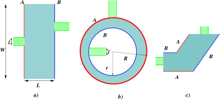
Figure 1: (Color online). Sketch of the geometries of a graphene quantum dot analyzed in the paper. a) Rectangular dot. b) Ring shaped dot. c) $60^{\circ}$ edge.

III Results

III.1 Rectangular dot

We first consider a rectangular dot, determined by its length $L$, and width $W$, as sketched in Fig.[1a]. Each of the leads be connected to an edge terminated in the $A$ sublattice, and the other be connected to an edge terminated in the $B$ sublattice.

For simplicity, we assume periodic boundary conditions along the vertical direction, as in Ref.Katsnelson (2006). For a graphene ribbon of width $W\gg a$, the solutions for open boundary conditions can be written as superpositions of waves with opposite momenta which are possible solutions of an equivalent problem with periodic boundary conditions. The difference between the two choices for a ribbon with $N$ unit cells of length $a$ lies in the set of allowed momenta, $k_{\perp}=n\pi/[(N+1)a],n=1,\cdots,N$ for periodic boundary conditions, and $k_{\perp}=\pm 2\pi n/(Na),n=0,\cdots,N/2$. If the transmissions to be calculated are a smooth function of the momentum $k_{\perp}$, the results obtained using either choice of boundary conditions converge to the same value for $N\gg 1$.

For the rectangular dot considered here, the $x$ coordinate lies within the range $-L/2\leq x\leq L/2$, and the $y$ coordinate can be written as $y=W\times\theta/(2\pi)$, with $0\leq\theta\leq 2\pi$. The wave functions inside the dot can be expanded using the basis:

$$\Psi(x,y)\equiv\sum_{n=-\infty}^{\infty}a_{n}\left(\begin{array}[]{c}e^{2\pi nz/W}\\ 0\end{array}\right)+b_{n}\left(\begin{array}[]{c}0\\ e^{2\pi n\bar{z}/W}\end{array}\right)$$ (18)

The incoming lead is attached at the position $z_{1}=-L/2$, and the outgoing lead is attached to the position $z_{2}=L/2+iW\times\theta_{0}/(2\pi)$. The contact averages out the details of the wave functions in the dot over a length of order $l$. Hence, the description of the effects of the contact does not require the infinite sum in Eq.(18). In the following, we include an upper cutoff, $n_{max}\approx W/l$. The boundary conditions at $z_{1}$ and $z_{2}$ are:

$$1+R = \sum_{n=-n_{max}}^{n_{max}}a_{n}e^{2\pi nz_{1}/W}=\sum_{n=-n_{max}}^{n_{max}}a_{n}e^{-\pi nL/W}$$

$$1-R = \sum_{n=-n_{max}}^{n_{max}}b_{n}e^{2\pi n\bar{z}_{1}/W}=\sum_{n=-n_{max}}^{n_{max}}b_{n}e^{-\pi nL/W}$$

$$T = \sum_{n=-n_{nmax}}^{n_{nmax}}a_{n}e^{2\pi nz_{2}/W}=\sum_{n=-n_{max}}^{n_{max}}a_{n}e^{\pi nL/W}e^{in\theta_{0}}$$

$$T = \sum_{n=-n_{max}}^{n_{max}}b_{n}e^{2\pi n\bar{z}_{2}/W}=\sum_{n=-n_{max}}^{n_{max}}b_{n}e^{\pi nL/W}e^{-in\theta_{0}}$$

The zigzag boundary conditions at points at the edge with $x=-L/2$ other than the position of the lead, $\theta=0$, and at the edge with $x=L/2$ for $\theta\neq\theta_{0}$ read:

$$\sum_{n=-n_{max}}^{n_{max}}b_{n}e^{-\pi nL/W}e^{-in\theta} =0 \,\,\,\,\,\,\,\theta\neq 0$$

$$\sum_{n=-n_{max}}^{n_{max}}a_{n}e^{\pi nL/W}e^{in\theta} =0 \,\,\,\,\,\,\,\theta\neq\theta_{0}$$ (20)

An Ansatz which is compatible with the two sets of boundary conditions is

$$a_{n} = Te^{-\pi nL/W}e^{-in\theta_{0}}$$

$$b_{n} = (1-R)e^{\pi nL/W}$$ (21)

which leads to the equations

$$1+R = T\sum_{n=-n_{max}}^{n_{max}}e^{-2\pi nL/W}e^{-in\theta_{0}}$$

$$1-R = T\left[\sum_{n=-n_{max}}^{n_{max}}e^{2\pi nL/W}\right]^{-1}$$ (22)

and

$$T=\frac{2}{\sum_{n=-n_{max}}^{n_{max}}e^{-2\pi nL/W}e^{-in\theta_{0}}+\left[\sum_{n=-n_{max}}^{n_{max}}e^{2\pi nL/W}\right]^{-1}}$$ (23)

The sums in Eq.(23) are dominated by the terms with $n\sim\pm n_{max}$. Hence, we obtain:

$$|T|^{2}\propto e^{-4\pi(L/W)(W/l)}$$ (24)

Finally, when the two contacts are attached to the same type of zigzag edge, the boundary conditions lead to either $a_{n}=0$ (contacts attached to an $A$ terminated edge) or $b_{n}=0$ (for a $B$ terminated edge), and, as a result, $R=1$ and $T=0$.

The assumption of a rectangular shape implies that the top and bottom boundaries may be of the armchair type, leading to intervalley mixingBrey and Fertig (2006). These boundaries are separated by a length $W\gg l$. The valley mixing induces a change in the allowed values of the transverse momentum, $k_{y}$, with respect to the case of zigzag boundary conditions. The momentum shift isBrey and Fertig (2006) $\Delta k_{y}\sim W^{-1}$. An incoming valley polarized mode can be written as a superposition of exact eigenmodes in the presence of valley mixing at the boundaries, with a spread in momentum of order $\Delta k_{y}\sim l^{-1}$.

As discussed above, the transmission through the dot is determined by evanescent waves with decay length $\kappa^{-1}\sim l$. The parallel momentum associated to these states is $k_{y}\sim\kappa\sim l^{-1}$. This superposition of valley polarized states will be changed by the existence of valley mixing at the top and bottom boundaries. The effects are of order $e^{-\Delta\kappa L}\sim e^{-L/W}$, which are exponentially smaller than the transmission coefficient obtained above, $|T|\sim e^{-4\pi L/l}$.

The previous analysis can be extended to a rectangular graphene quantum dot in a constant magnetic field. The wave functions in Eq.(18) in this case become

$$\Psi(x,y) \equiv \sum_{n=-n_{max}}^{n_{max}}a_{n}\left(\begin{array}[]{c}e^{2\pi in/W}e^{-x^{2}/(2l_{B}^{2})}\\ 0\end{array}\right)+$$ (27)

$$+ b_{n}\left(\begin{array}[]{c}0\\ e^{2\pi in/W}e^{x^{2}/(2l_{B}^{2})}\end{array}\right)$$ (30)

where $l_{B}=\sqrt{\hbar c\ |e|B}$ is the magnetic length, $B$ is the magnetic induction. The same manipulations described above allow us to calculate the transmission coefficient, which turns out to be unchanged with respect to Eq.(24). The lack of dependence of the transmission on the applied field is in agreement with the insensitivity of the bulk transport to the magnetic field when the chemical potential is at the Dirac pointPrada et al. (2007).

III.2 Circular dot

We now consider a ring-shaped dot, with the contacts attached to the inner and outer edges, which are assumed to be $A$ and $B$ terminated, respectivelyWunsch et al. (2008). As discussed there, a graphene dot with an approximate circular shape can be bounded by different edges where the majority sublattice is of either type. The advantage of assuming the same boundary conditions throughout the edge is that the problem retains circular symmetry, and the solutions have a well defined angular momentum, $l$, where $l=1,\cdots l_{max}\approx R/a$, where $R$ is the radius of the dot and $a$ is the lattice constant. For $R/a\gg 1$, superpositions of wavefunctions with $l\gg 1$ can be built, with a small spread in angles, $\Psi(r,\theta)\neq 0$ only if $\theta_{0}-\Delta\theta\leq\theta\leq\theta_{0}+\Delta\theta$, with $\Delta\theta\ll 2\pi$. These states are solutions of the Dirac equation at zero energy which are not affected by the global properties of the boundaries of the dot. Hence, they can be used to describe transport between positions at the dot edges which are close enough so as to be insensitive to the global properties of the edges. The case when the transport properties are influenced by the type of edges requires input about features at distances comparable to the lattice spacing, and will be considered in the next subsection.

The outer and inner radii are $R_{1}$ and $R_{2}$, as shown in Fig.[1b]. The modes at $\epsilon=0$ inside the dot which satisfy the boundary conditions can be obtained by a conformal transformation which changes the rectangular (cylindrical) dot considered in the previous subsection into a ring. This transformation is

$$w(z)=\sqrt{R_{1}R_{2}}e^{2\pi iz/W}$$ (31)

and $e^{2\pi L/W}=R_{1}/R_{2}$. Using this transformation, the wave functions in Eq.(18) become

$$\Psi(x,y)\equiv\sum_{n=-\infty}^{\infty}a_{n}\left(\begin{array}[]{c}z^{n}\\ 0\end{array}\right)+b_{n}\left(\begin{array}[]{c}0\\ \bar{z}^{n}\end{array}\right)$$ (32)

The size of the contact, $l$, induces a maximum value $n$, $n_{max}\sim 2\pi R_{2}/l$. From the wave functions in Eq.(32), and using the same analysis as for the rectangular dot in the previous subsection, we wind, in analogy with Eq.(24):

$$|T|^{2}\sim\left(\frac{R_{2}}{R_{1}}\right)^{8\pi R_{2}/l}$$ (33)

If we write $2\pi R_{2}=W$ and $R_{1}\approx R_{2}+L$, this expression reduces to Eq.(24) when $R_{1}\sim R_{2}\gg R_{1}-R_{2}$.

As in the case of the rectangular dot, the only allowed solution when the two contacts are attached to the same boundary is $R=1$ and $T=0$.

Dots of different shapes can be obtained using other conformal transformations. For instance, the circular dot analyzed here can be turned into a dot with a corrugated boundary using the mapping

$$w^{\prime}(w)=w+\lambda w^{m}$$ (34)

where $m$ fixes the period of the corrugation, and $\lambda\propto\delta R/R^{m}$ gives its amplitude. The transmission coefficient in eq.(33) acquires corrections of order $(R/l)(\delta R/R)^{m}$.

This analysis can also be extended to a finite magnetic field. In that case the wave functions are

$$\Psi(x,y) \equiv \sum_{n=-n_{max}}^{n_{max}}a_{n}\left(\begin{array}[]{c}z^{n}e^{-r^{2}/(2l_{B}^{2})}\\ 0\end{array}\right)+$$ (37)

$$+ b_{n}\left(\begin{array}[]{c}0\\ \bar{z}^{n}e^{r^{2}/(2l_{B}^{2})}\end{array}\right)$$ (40)

The boundary conditions imply

$$1+R = e^{-R_{1}^{2}/(2l_{B}^{2})}\sum_{n=-n_{max}}^{n_{max}}a_{n}R_{1}^{n}$$

$$1-R = e^{R_{1}^{2}/(2l_{B}^{2})}\sum_{n=-n_{max}}^{n_{max}}b_{n}R_{1}^{n}$$

$$T = e^{-R_{2}^{2}/(2l_{B}^{2})}\sum_{n=-n_{max}}^{n_{max}}a_{n}R_{2}^{n}e^{in\theta_{0}}$$

$$T = e^{R_{2}^{2}/(2l_{B}^{2})}\sum_{n=-n_{max}}^{n_{max}}b_{n}R_{2}^{n}e^{-in\theta_{0}}$$ (41)

A possible solution is of the form

$$b_{n} = \frac{C}{R_{2}^{n}}e^{in\theta_{0}}$$

$$a_{n} = \frac{A}{R_{1}^{n}}$$ (42)

leading to the equations

$$1+R = Ae^{-R_{1}^{2}/(2l_{B}^{2})}n_{max}$$

$$1-R = Ce^{R_{1}^{2}/(2l_{B}^{2})}\left(\frac{R_{1}}{R_{2}}\right)^{n_{max}}$$

$$T = Ae^{-R_{2}^{2}/(2l_{B}^{2})}\left(\frac{R_{2}}{R_{1}}\right)^{n_{max}}e^{-in_{max}\theta_{0}}$$

$$T = Ce^{R_{2}^{2}/(2l_{B}^{2})}n_{max}$$ (43)

Thus, the transmission coefficient is

$$\left|T\right|^{2} = n_{max}^{2}\left(\frac{R_{2}}{R_{1}}\right)^{2n_{max}}e^{-(R_{1}^{2}-R_{2}^{2})/l_{B}^{2}}=$$ (44)

$$= n_{max}^{2}\left(\frac{R_{2}}{R_{1}}\right)^{2n_{max}}e^{-\Phi/\Phi_{0}}$$

where $\Phi$ is the magnetic flux per ring and $\Phi_{0}=\pi\hbar c/|e|$ is the flux quantum. The dependence of transport through the quantum dot on the magnetic field is exponential, rather than oscillatory as in case of the standard Aharonov-Bohm effectBeenakker and van Houten (1991), which reflects a specifics of transport via evanescent waves.

Thus, the conductance of circular quantum dot turns out to be very sensitive to the flux through the ring. This can be potentially interesting in light of development of magnetic sensors for measurements of very low fields without use of superconductivity.

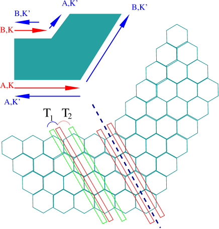
Figure 2: (Color online). Sketch of the $60^{\circ}$ junction analyzed in the text. Top left: an incoming wave from the left, built up from eigenstates in the vicinity of the $K$ valley has to be either transmitted or reflected as a superposition of states from the $K^{\prime}$ valley. Bottom: Scheme used to analyze the transmission in the honeycomb lattice. The junction has a reflection symmetry around its center, shown as dashed line. On each side, the nearest neighbor hopping problem can be written as a sum of coupling between nearest neighbor transverse stripes. See text for details.

III.3 Corner between two facets

We finally consider a 60^∘ angle boundary between an edge with $A$ termination, and an edge with $B$ termination, as sketched in Fig.[1c]. The leads are attached at distances $l_{1}$ and $l_{2}$ from the corner. The transmission along a ribbon with this geometry has been analyzed numerically in Refs.Rycerz and Beenakker (2007); Rycerk (2008); Iyengar et al. (2008). A full solution cannot be obtained within the continuum approximation, as in the previous cases, since both transmission and reflection at the wedge require Umklapp processes changing the valley index of the incoming electron. In this respect, the problem is similar to that of the transmission across a p-n junction near the Dirac pointAkhmerov et al. (2007).

We consider the ribbon with an angle shown in Fig.[2]. The system has reflection symmetry around an axis which connects the vortices of the angles at both sides. Far away from the corner, the system reduces to a zigzag ribbon. We assume that the edges of the ribbon are at $y=\pm W/2$, and $W\gg a$, where $a$ is the lattice constant. The wave function of an incoming wave can be written as

$$\Psi_{K}^{in}(x,y)\equiv\left(\begin{array}[]{c}\sinh\left[\kappa\left(y-\frac{W}{2}\right)\right]\\ -\sqrt{\frac{k+\kappa}{k-\kappa}}e^{\kappa(y-W/2)}+\sqrt{\frac{k-\kappa}{k+\kappa}}e^{\kappa(W/2-y)}\end{array}\right)e^{ikx}$$ (45)

where $\kappa$ and the energy of the state are given by:

$$\kappa = k\tanh\left(\kappa W\right)$$

$$\epsilon_{k} = v_{\rm F}\sqrt{k^{2}-\kappa^{2}}$$ (46)

For $kW\gg 1$, we find

$$\kappa \approx k(1-e^{-2kW}+\cdots)$$

$$\epsilon_{k} \approx v_{\rm F}ke^{-kW}$$ (47)

The solution (45) is valid for $k\geq W^{-1}$.

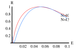
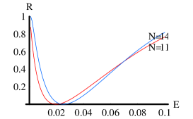
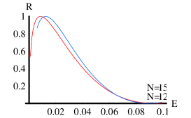
Figure 3: (Color online). Reflection at a 60^∘ junction like the one sketched in Fig.[2] for different junction widths. $N$ gives the number of unit cells across the junction. The width of each ribbon which make up the junction is $3/2aN$, where $a$ is the length of the C-C bond. The energy is in units of the nearest neighbor hopping.

Figure 4: (Color online). Weights of the wavefunction passing through the junction sketched in Fig.[2] on evanescent waves of different decay lengths. The width of the junction is 16 unit cells, and there are 30 evanescent waves. The decay length is in units of the lattice spacing in the direction parallel to the edges ($\sqrt{3}\times a$, where $a$ is the C-C bond). Diamonds show waves symmetric around the junction, and hexagons show antisymmetric waves (note that the waves studied here decay as function of the distance to the junction, not to the edges of the ribbon).

The reflected and transmitted waves can be written as in Eq.(45), except that, for the reflected wave the momentum is reversed, and the wave packet is built up from electrons at the $K^{\prime}$ valley:

$$\Psi_{K^{\prime}}^{ref}(x,y)\equiv\left(\begin{array}[]{c}\sinh\left[\kappa\left(y-\frac{W}{2}\right)\right]\\ -\sqrt{\frac{k+\kappa}{k-\kappa}}e^{\kappa(y-W/2)}+\sqrt{\frac{k-\kappa}{k+\kappa}}e^{\kappa(W/2-y)}\end{array}\right)e^{-ikx}$$ (48)

This wave function has to be matched to that in Eq.(45) at the interface. In the continuum limit, the overlap between wave functions at $K$ and $K^{\prime}$ valleys is zero, and the matching cannot be carried out. We analyze the corrections induced by the finite lattice by dividing each ribbon reaching the junction into stripes, as sketched in Fig.[2]. Using a nearest-neighbor tight-binding model, each one-dimensional ribbon is coupled to its two nearest neighbors, and the Hamiltonian can be written as a sum of $N\times N$ terms, $T_{1}$ and $T_{2}$, where $N$ is the number of atoms within each ribbon:

$$\epsilon_{k}\alpha_{i}^{M} = \sum_{j=1}^{N}T^{1}_{ij}\beta_{j}^{M}+T^{2}_{ij}\beta_{j}^{M+1}\,\,\,\,\,\,\,\,\,\,i=1,\cdots,N$$

$$\epsilon_{k}\beta_{i}^{M} = \sum_{j=1}^{N}T^{1}_{ij}\alpha_{j}^{M}+T^{2}_{ij}\alpha_{j}^{M-1}\,\,\,\,\,\,\,\,\,\,i=1,\cdots,N$$ (49)

where $M$ is a stripe index.

Using the inversion symmetry of the junction, we can analyze separately states which are even and odd with respect to the axis which joins the two angles of the junction. Within each subsector, the problem is reduced to the reflection of an incoming wave of energy $\epsilon_{k}$ at a sharp boundary at the location of the junction. The coupling between the stripes at each side of the junction becomes, in the new geometry, an energy shift equal to the hopping $t$ at the atoms in the last stripe of the system:

$$\epsilon_{k}\alpha_{i}^{0}=\pm t\alpha_{i}^{0}+\sum_{j=1}^{N}T^{1}_{ij}\beta_{j}^{0}\,\,\,\,\,\,\,\,\,\,i=1,\cdots,N$$ (50)

An incoming wave of momentum $k$ and energy $\epsilon_{k}$ defines a set of coefficients, $\{\alpha_{i}^{k}\},\{\beta_{i}^{k}\}$, such that the Ansatz:

$$\alpha_{i}^{M} = \alpha_{i}^{k}e^{ikM}$$

$$\beta_{i}^{M} = \beta_{i}^{k}e^{ikM}$$ (51)

is a solution of Eq.(49). In the limit $N\gg 1$, and $\epsilon_{k}\ll t$, these amplitudes are well approximated by Eq.(45). For a given energy $\epsilon_{k}\sim te^{-N}$, we can define only one incoming and outgoing set of amplitudes as in Eq.(51). We can also define $N-1$ amplitudes $\{\alpha_{i}^{\kappa}\},\{\beta_{i}^{\kappa}\}$ such that

$$\alpha_{i}^{M} = \alpha_{i}^{k}e^{-\kappa M}$$

$$\beta_{i}^{M} = \beta_{i}^{k}e^{-\kappa M}$$ (52)

satisfy Eq.(49). For energies very near the Dirac point, the solutions (51) and (52) are such that either the amplitudes $\alpha_{i}^{k},\alpha_{i}^{\kappa}$ or $\beta_{j}^{k},\beta_{j}^{\kappa}$ are exponentially small when $T^{1}_{i,j},T^{2}_{ij}\neq 0$.

The boundary condition at the edge of the system is given by Eq.(50) where the amplitudes can be expanded into an incoming, a reflected, and $M_{1}$ evanescent waves:

$$\alpha_{i}^{0} =\alpha_{i}^{k}+R\alpha_{i}^{-k}+\sum_{\kappa}C_{\kappa}\alpha_{i}^{\kappa}$$

$$\beta_{i}^{0} =\beta_{i}^{k}+R\beta_{i}^{-k}+\sum_{\kappa}C_{\kappa}\beta_{i}^{\kappa}$$ (53)

The insertion of these expressions into Eq.(50) leads to $N$ equations with the $N-1$ unknowns $\{C_{\kappa}\}$, and the reflection coefficient $R$. The even and odd combinations of the initial junction problem allows us to define to reflection coefficients, $R_{\pm}$ obtained using the two possible signs in Eq.(50). It is easy to show that the transmission coefficient of the junction can be written as $T=(R_{+}-R_{-})/2$.

The only solution of Eq.(50) at low energies requires all the amplitudes $\alpha_{i}^{0}$ to be exponentially small, as a finite set of values $\alpha_{i}^{0}$ and $\beta_{j}^{0}$ are incompatible if $T^{1}_{ij}\neq 0$. Hence, the parameters $C_{\kappa}^{\pm}$ and $R_{\pm}$ are determined by a set of equations which are independent of the choice of sign in Eq.(50), so that $R_{+}\approx R_{-}$ with exponential accuracy. Hence, the transmission coefficient of the original junction also vanishes with exponential accuracy, in agreement with the numerical calculations in Refs.Rycerz and Beenakker (2007); Rycerk (2008).

Results are shown in Fig.[3]. They are consistent with those reported inIyengar et al. (2008). The dependence on energy of the reflection coefficient shows three characteristic patterns, which are repeated as function of the width of the junction, as shown in the Figure. This approximate periodicity is reminiscent of the alternance of metallic and non metallic features in carbon nanotubes and graphene nanoribbons.

The calculation described here requires the existence of evanescent waves which have a finite overlap with wavepackets derived from both the $K$ and $K^{\prime}$ points of the Brillouin zone, in a similar way to the transmission problem analyzed in Ref.Akhmerov et al. (2007). The coupling between the two valleys can be analyzed in detail by calculating the relative weights of the different evanescent waves which must be defined at the junction. Results for a junction of width $N=16$ are shown in Fig.[4], where the decay length is defined as $l_{ev}=1/\kappa$ in eq.(52). Most of the weight is concentrated on evanescent waves with a short decay length, which cannot be ascribed to a given valley.

IV Conclusions

We have studied the transmission, at zero energy, through graphene quantum dots attached to leads with one incoming and outgoing channels, extending the analysis in Refs.Katsnelson (2006); Tworzydo et al. (2006). We assume that, for energies at distances to the Dirac point smaller than $v_{\rm F}/L$, where $L$ is the typical dimension of the system, extended states can be neglected, and the electronic properties are mainly determined by evanescent waves, or by localized states induced by boundaries.

We have shown that the dots of various shapes can be analyzed, using conformal transformations which preserve the nature of the states at zero energy. An exception is an angle between zigzag boundaries with different terminations, where the solution of the problem requires the analysis of evanescent waves which do not have a well defined valley index, and cannot be described by the continuum Dirac equation.

We find that:

(i) The transmission vanishes when the leads are attached to the same edge.

(ii) The transmission depends exponentially on the ratio between the size of the dot and the width of the contact.

(iii) The shape of the dot changes significantly the transmission.

(iv) The effects of a magnetic field are strongly dependent on the shape of the dot. A rectangular dot is unique in that a magnetic field does not change the transport properties (see alsoPrada et al. (2007)). In general, the conduction of the dot is very sensitive to the magnetic flux through it. A similar behavior for dots in the diffusive regime has been reported inAbanin and Levitov (2008).

(v) The transmission when the two contacts are attached to an edge such that both the transmitted and reflected wave belong to the opposite valley as the incoming wave depends on the lattice structure at short distances.

V Acknowledgements

This work was supported by MEC (Spain) through grant FIS2005-05478-C02-01 and CONSOLIDER CSD2007-00010, the Comunidad de Madrid, through the program CITECNOMIK, CM2006-S-0505-ESP-0337, the European Union Contract 12881 (NEST), and the Stichting voor Fundamenteel Onderzoek der Materie (FOM) (the Netherlands). We appreciate helpful conversations with L. Brey and M. A. H. Vozmediano.

References

- Novoselov et al. (2004) K. S. Novoselov, A. K. Geim, S. V. Morozov, D. Jiang, Y. Zhang, S. V. Dubonos, I. V. Grigorieva, and A. A. Firsov, Science 306, 666 (2004).
- Novoselov et al. (2005) K. S. Novoselov, D. Jiang, F. Schedin, T. J. Booth, V. V. Khotkevich, S. V. Morozov, and A. K. Geim, Proc. Nat. Acad. Sc. 102, 10451 (2005).
- Geim and Novoselov (2007) A. K. Geim and K. S. Novoselov, Nature Materials 6, 183 (2007).
- Katsnelson and Novoselov (2007) M. I. Katsnelson and K. S. Novoselov, Sol. State Commun. 143, 3 (2007).
- Castro Neto et al. (2007) A. H. Castro Neto, F. Guinea, N. M. R. Peres, K. S. Novoselov, and A. K. Geim (2007), Rev. Mod. Phys., in press, eprint arXiv:0709.1163.
- Katsnelson (2006) M. I. Katsnelson, Eur. J. Phys. B 51, 157 (2006).
- Tworzydo et al. (2006) J. Tworzydo, B. Trauzettel, M. Titov, A. Rycerz, and C. W. J. Beenakker, Phys. Rev. Lett. 96, 246802 (2006).
- Miao et al. (2007) F. Miao, S. Wijeratne, Y. Zhang, U. C. Coskun, W. Bao, and C. N. Lau, Science 317, 1530 (2007).
- Danneau et al. (2008) R. Danneau, F. Wu, M. F. Craciun, S. Russo, M. Y. Tomi, J. Salmilehto, A. F. Morpurgo, and P. J. Hakonen (2008), eprint arXiv:0711.4306.
- Fujita et al. (1996) M. Fujita, K. Wakabayashi, K. Nakada, and K. Kusakabe, J. Phys. Soc. Jpn. 65, 1920 (1996).
- Vozmediano et al. (2005) M. A. Vozmediano, M. P. López-Sancho, T. Stauber, and F. Guinea, Phys. Rev. B 72, 155121 (2005).
- Pereira et al. (2006) V. M. Pereira, F. Guinea, J. M. Lopes dos Santos, N. M. Peres, and A. H. Castro Neto, Phys. Rev. Lett. 96, 036801 (2006).
- Akhmerov and Beenakker (2008) A. R. Akhmerov and C. W. J. Beenakker, Phys. Rev. B 77, 085423 (2008).
- Guinea et al. (2008) F. Guinea, M. I. Katsnelson, and M. A. H. Vozmediano, Phys. Rev. B 77, 075422 (2008).
- Louis et al. (2007) E. Louis, J. A. Vergés, F. Guinea, and G. Chiappe, Phys. Rev. B 75, 085440 (2007).
- Titov (2007) M. Titov, Europhys. Lett. 79, 17004 (2007).
- Wunsch et al. (2008) B. Wunsch, T. Stauber, and F. Guinea, Phys. Rev. B 77, 035316 (2008).
- Bunch et al. (2005) J. S. Bunch, Y. Yaish, M. Brink, K. Bolotin, and P. L. McEuen, Nano Lett. 5, 2887 (2005).
- Han et al. (2007) M. Y. Han, B. Özyilmaz, Y. Zhang, and P. Kim, Phys. Rev. Lett. 98, 206805 (2007).
- Avouris et al. (2007) P. Avouris, Z. Chen, and V. Perebeinos, Nature Nanotechnology 2, 605 (2007).
- Ponomarenko et al. (2008) L. A. Ponomarenko, F. Schedin, M. I. Katsnelson, R. Yang, E. H. Hill, K. S. Novoselov, and A. K.Geim, Science 320, 356 (2008).
- Brey and Fertig (2006) L. Brey and H. A. Fertig, Phys. Rev. B 73, 235411 (2006).
- Prada et al. (2007) E. Prada, P. San-José, B. Wunsch, and F. Guinea, Phys. Rev. B 75, 113407 (2007).
- Beenakker and van Houten (1991) C. W. J. Beenakker and H. van Houten, Sol. St. Phys. 44, 1 (1991).
- Rycerz and Beenakker (2007) A. Rycerz and C. W. J. Beenakker (2007), eprint arXiv:0709.3397.
- Rycerk (2008) A. Rycerk, Phys. St. Sol. (a) 205, 1281 (2008).
- Iyengar et al. (2008) A. Iyengar, T. Luo, H. A. Fertig, and L. Brey (2008), eprint arXiv:0804.0246.
- Akhmerov et al. (2007) A. R. Akhmerov, J. H. Bardarson, A. Rycerz, and C. W. J. Beenakker, Phys. Rev. B 77, 205416 (2007).
- Abanin and Levitov (2008) D. A. Abanin and L. S. Levitov, Phys. Rev. B 78, 035416 (2008).