Power Series Composition and Change of Basis

Abstract

Efficient algorithms are known for many operations on truncated power series (multiplication, powering, exponential, …). Composition is a more complex task. We isolate a large class of power series for which composition can be performed efficiently. We deduce fast algorithms for converting polynomials between various bases, including Euler, Bernoulli, Fibonacci, and the orthogonal Laguerre, Hermite, Jacobi, Krawtchouk, Meixner and Meixner-Pollaczek.

Categories and Subject Descriptors:
I.1.2 [Computing Methodologies]:  Symbolic and Algebraic Manipulation – Algebraic Algorithms

General Terms: Algorithms, Theory

Keywords: Fast algorithms, transposed algorithms, basis conversion, orthogonal polynomials.

1 Introduction

Through the Fast Fourier Transform, fast polynomial multiplication has been the key to devising efficient algorithms for polynomials and power series. Using techniques such as Newton iteration or divide-and-conquer, many problems have received satisfactory solutions: polynomial evaluation and interpolation, power series exponentiation, logarithm, … can be performed in quasi-linear time.

In this article, we discuss two questions for which such fast algorithms are not known: power series composition and change of basis for polynomials. We isolate special cases, including most common families of orthogonal polynomials, for which our algorithms reach quasi-optimal complexity.

Composition. Given a power series $g$ with coefficients in a field $\mathbb{K}$, we first consider the map of evaluation at $g$

$$\mathsf{Eval}_{m,n}(.,g):A\in\mathbb{K}[x]_{m}\mapsto A(g)\bmod x^{n}\in\mathbb{K}[x]_{n}.$$

Here, $\mathbb{K}[x]_{m}$ is the $m$-dimensional $\mathbb{K}$-vector space of polynomials of degree less than $m$. We note $\mathsf{Eval}_{n}$ for $\mathsf{Eval}_{n,n}$.

To study this problem, as usual, we denote by $\mathsf{M}$ a multiplication time function, such that polynomials of degree less than $n$ can be multiplied in $\mathsf{M}(n)$ operations in $\mathbb{K}$. We impose the usual super-linearity conditions of [17, Chap. 8]. Using Fast Fourier Transform algorithms, $\mathsf{M}(n)$ can be taken in $O(n\log(n))$ over fields with suitable roots of unity, and $O(n\log(n)\log\log(n))$ in general [31, 14].

If $g(0)=0$, the best known algorithm, due to Brent and Kung, uses $O(\sqrt{n\log n}\,\mathsf{M}(n))$ operations in $\mathbb{K}$ [11]; in small characteristic, a quasi-linear algorithm is known [5]. There are however special cases of power series $g$ with faster algorithms: evaluation at $g=\lambda x$ takes linear time; evaluation at $g=x^{k}$ requires no arithmetic operation. A non-trivial example is $g=x+a$, which takes time $O(\mathsf{M}(n))$ when the base field has characteristic zero or large enough [1]. Brent and Kung [11] also showed how to obtain a cost in $O(\mathsf{M}(n)\log(n))$ when $g$ is a polynomial; this was extended by van der Hoeven [22] to the case where $g$ is algebraic over $\mathbb{K}(x)$. In §2, we prove that evaluation at $g=\exp(x)-1$ and at $g=\log(1+x)$ can also be performed in $O(\mathsf{M}(n)\log(n))$ operations over fields of characteristic zero or larger than $n$.

Using associativity of composition and the linearity of the map $\mathsf{Eval}_{m,n}$, we show in §2 how to use these special cases as building blocks, to obtain fast evaluation algorithms for a large class of power series. This idea was first used by Pan [28], who applied it to functions of the form $(ax+b)/(cx+d)$. Our extensions cover further examples such as $2x/(1+x)^{2}$ or $(1-\sqrt{1-x^{2}})/x$, for which we improve the previously known costs.

Bivariate problems. Our results on the cost of evaluation (and of the transposed operation) are applied in §3 to special cases of a more general composition, reminiscent of umbral operations [30]. Given a bivariate power series $\mathbf{F}=\sum_{j\geq 0}\xi_{j}(x)t^{j}$, we consider the linear map

$$\mathsf{Eval}_{n}(.,\mathbf{F},t):(a_{0},\dots,a_{n-1})\mapsto\sum_{j<n}\xi_{j}(x)a_{j}\bmod x^{n}.$$

For instance, with

$$\mathbf{F}=\frac{1}{1-tg(x)}=\sum_{j\geq 0}g(x)^{j}t^{j},$$

this is the map $\mathsf{Eval}_{n}(.,g)$ seen before. For general $\mathbf{F}$, the conversion takes quadratic time (one needs $n^{2}$ coefficients for $\mathbf{F}$). Hence, better algorithms can only been found for structured cases; in §3, we isolate a large family of bivariate series $\mathbf{F}$ for which we can provide such fast algorithms. This approach follows Frumkin’s [16], which was specific to Legendre polynomials.

Change of basis. Our framework captures in particular the generating series of many classical polynomial families, for which it yields at once conversion algorithms between the monomial and polynomial bases, in both directions.

Thus, we obtain in §4 change of basis algorithms of cost only $O(\mathsf{M}(n))$ for all of Jacobi, Laguerre and Hermite orthogonal polynomials, as well as Euler, Bernoulli, and Mott polynomials (see Table 4). These algorithms are derived in a uniform manner from our composition algorithms; they improve upon the existing results, of cost $O(\mathsf{M}(n)\log(n))$ or $O(\mathsf{M}(n)\log^{2}(n))$ at best (see below for historical comments).

We also obtain $O(\mathsf{M}(n)\log(n))$ conversion algorithms for a large class of Sheffer sequences [30, Chap. 2], including actuarial polynomials, Poisson-Charlier polynomials and Meixner polynomials (see Table 4).

Transposition. A key aspect of our results is their heavy use of transposed algorithms. Introduced under this name by Kaltofen and Shoup, the transposition principle is an algorithmic theorem with the following content: given an algorithm that performs an $r\times s$ matrix-vector product $b\mapsto Mb$, one can deduce an algorithm with the same complexity, up to $O(r+s)$ operations, and that performs the transposed matrix-vector product $c\mapsto M^{t}c$. In other words, this relates the cost of computing a $\mathbb{K}$-linear map $f:\ V\to W$ to that of computing the transposed map $f^{t}:\ W^{*}\to V^{*}$.

For the transposition principle to apply, some restrictions must be imposed on the computational model: we require that only linear operations in the coefficients of $b$ are performed (all our algorithms satisfy this assumption). See [12] for a precise statement, Kaltofen’s “open problem” [23] for further comments and [7] for a systematic review of some classical algorithms from this viewpoint.

To make the design of transposed algorithms transparent, we choose as much as possible to describe our algorithms in a “functional” manner. Most of our questions boil down to computing linear maps $\mathbb{K}[x]_{m}\to\mathbb{K}[x]_{n}$; expressing algorithms as a factorization of these maps into simpler ones makes their transposition straightforward. In particular, this leads us to systematically indicate the dimensions of the source (and often target) space as a subscript.

Previous work. The question of efficient change of basis has naturally attracted a lot of attention, so that fast algorithms are already known in many cases.

Gerhard [18] provides $O(\mathsf{M}(n)\log(n))$ conversion algorithms between the falling factorial basis and the monomial basis: we recover this as a special case. The general case of Newton interpolation is discussed in [6, p. 67] and developed in [9]. The algorithms have cost $O(\mathsf{M}(n)\log(n))$ as well.

More generally, if $(P_{i})$ is a sequence of polynomials satisfying a recurrence relation of fixed order (such as an orthogonal family), the conversion from $(P_{i})$ to the monomial basis $(x^{i})$ can also be computed in $O(\mathsf{M}(n)\log(n))$ operations: an algorithm is given in [29], and an algorithm for the transpose problem is in [15]. Both operate on real or complex arguments, but the ideas extend to more general situations. Alternative algorithms, based on structured matrices techniques, are given in [21]. They perform conversions in both directions in cost $O(\mathsf{M}(n)\log^{2}(n))$.

The overlap with our results is only partial: not all families satisfying a fixed order recurrence relation fit in our framework; conversely, our method applies to families which do not necessarily satisfy such recurrences (the work-in-progress [8] specifically addresses conversion algorithms for orthogonal polynomials).

Besides, special algorithms are known for converting between particular families, such as Chebyshev, Legendre and Bézier [27, 4], with however a quadratic cost. Floating-point algorithms are known as well, of cost $O(n)$ for conversion from Legendre to Chebyshev bases [2] and $O(n\log(n))$ for conversions between Gegenbauer bases [25], but the results are approximate. Approximate conversions for the Hermite basis are discussed in [26], with cost $O(\mathsf{M}(n)\log(n))$.

Note on the base field. For the sake of simplicity, in all that follows, the base field is supposed to have characteristic 0. All results actually hold more generally, for fields whose characteristic is sufficiently large with respect to the target precision of the computation. However, completely explicit estimates would make our statements cumbersome.

2 Composition

Associativity of composition can be read both ways: in the identity $A(f\circ g)=A(f)\circ g$, $f$ is either composed on the left of $g$ or on the right of $A$. In this section, we discuss the consequences of this remark. We first isolate a class of operators $f$ for which both left and right composition can be computed fast. Most results are known; we introduce two new ones, regarding exponentials and logarithms. Using these as building blocks, we then define composition sequences, which enable us to obtain more complex functions by iterated compositions. We finally discuss the cost of the map $\mathsf{Eval}_{n}$ and of its inverse for such functions, showing how to reduce it to $O(\mathsf{M}(n))$ or $O(\mathsf{M}(n)\log(n))$.

2.1 Basic Subroutines

We now describe a few basic subroutines that are the building blocks in the rest of this article.

Left operations on power series. In Table 1, we list basic composition operators, defined on various subsets of $\mathbb{K}[[x]]$. Explicitly, any such operator $\mathsf{o}$ is defined on a domain $\mathsf{dom}(\mathsf{o})$, given in the third column. Its action on a power series $g\in\mathsf{dom}(\mathsf{o})$ is given in the second column, and the cost of computing $\mathsf{o}(g)\bmod x^{n}$ is given in the last column.

Operator	Action	Domain	Cost
$\mathsf{A}_{a}$ (add)	$a+g$	$\mathbb{K}[[x]]$	1
$\mathsf{M}_{\lambda}$ (mul)	$\lambda g$	$\mathbb{K}[[x]]$	$n$
$\mathsf{P}_{k}$ (power)	$g^{k}$	$\mathbb{K}[[x]]$	$O(\log k+\mathsf{M}(n))$
$\mathsf{R}_{k,\alpha,r}$ (root)	$g^{1/k}$	$\alpha^{k}x^{rk}(1+x\mathbb{K}[[x]])$	$O(\mathsf{M}(n))$
$\mathsf{Inv}$ (inverse)	$1/g$	$\mathbb{K}^{*}+x\mathbb{K}[[x]]$	$O(\mathsf{M}(n))$
$\mathsf{E}$ (exp.)	$\exp(g)-1$	$x\mathbb{K}[[x]]$	$O(\mathsf{M}(n))$
$\mathsf{L}$ (log.)	$\log(1+g)$	$x\mathbb{K}[[x]]$	$O(\mathsf{M}(n))$

Table 1: Basic Operations on Power Series

Some comments are in order. For addition and multiplication, we take $a\in\mathbb{K}$ and $\lambda$ in $\mathbb{K}^{*}$. To lift indeterminacies, the value of $\mathsf{R}_{k,\alpha,r}(g)$ is defined as the unique power series with leading term $\alpha x^{r}$ whose $k$th power is $g$; observe that to compute $\mathsf{R}_{k,\alpha,r}(g)\bmod x^{n}$, we need $g$ modulo $x^{n+r(k-1)}$ as input. Finally, we choose to subtract 1 to the exponential so as to make it the inverse of the logarithm. All complexity results are known; they are obtained by Newton iteration [10].

Right operations on polynomials. In Table 2, we describe a few basic linear maps on $\mathbb{K}[x]_{m}$ (observe that the dimension $m$ of the source is mentioned as a subscript). Their action on a polynomial

$$A(x)=a_{0}+\dots+a_{m-1}x^{m-1}\in\mathbb{K}[x]_{m}$$

is described in the third column. In the case of powering, it is assumed that $k\in\mathbb{N}_{>0}$. Here and in what follows, we freely identify $\mathbb{K}[x]_{m}$ and $\mathbb{K}^{m}$, through the isomorphism

$$\sum_{i<m}a_{i}x^{i}\in\mathbb{K}[x]_{m}\ \leftrightarrow\ (a_{0},\dots,a_{m-1})\in\mathbb{K}^{m}.$$

Name	Notation	Action	Cost
Powering	$\mathsf{Power}_{m,k}$	$A(x^{k})$	0
Reversal	$\mathsf{Rev}_{m}$	$x^{m-1}A(1/x)$	0
Mod	$\mathsf{mod}_{m,n}$	$A\bmod x^{n}$	0
Scale	$\mathsf{Scale}_{\lambda,m}$	$A(\lambda x)$	$O(m)$
Diagonal	$\mathsf{\Delta}_{m}(.,s_{i})$	$\sum{a_{i}s_{i}x^{i}}$	$m$
Multiply	$\mathsf{Mul}_{m,n}(.,P)$	$AP\bmod x^{n}$	$~{}\mathsf{M}(\max(n,m))$
Shift	$\mathsf{Shift}_{a,m}$	$A(x+a)$	$\mathsf{M}(m)+O(m)$

Table 2: Basic Operations on Polynomials

All of the cost estimates are straightforward, except for the shift, which, in characteristic 0, can be deduced from the other ones by the factorization [1]:

$$\mathsf{Shift}_{a,m}=\mathsf{\Delta}_{m}(\mathsf{Rev}_{m}(\mathsf{Mul}_{m,m}(\mathsf{Rev}_{m}(\mathsf{\Delta}_{m}(.,i!)),P)),1/i!),$$

where $P$ is the polynomial $\sum_{i=0}^{n-1}a^{i}x^{i}/i!$. We continue with some equally simple operators, whose description however requires some more detail. For $k\in\mathbb{N}_{>0}$, any polynomial $A$ in $\mathbb{K}[x]$ can be uniquely written as

$$A(x)=A_{0/k}(x^{k})+A_{1/k}(x^{k})x+\cdots+A_{k-1/k}(x^{k})x^{k-1}.$$

Inspecting degrees, one sees that if $A$ is in $\mathbb{K}[x]_{m}$, then $A_{i/k}$ is in $\mathbb{K}[x]_{m_{i}}$, with

$$m_{i}=\lfloor{m/k}\rfloor+\begin{cases}1&\text{if $i\leq m\bmod k$,}\\ 0&\text{otherwise.}\end{cases}$$ (1)

This leads us to define the map $\mathsf{Split}_{m,k}:$

$$A\in\mathbb{K}[x]_{m}\mapsto(A_{0/k},\dots,A_{k-1/k})\in\mathbb{K}[x]_{m_{0}}\times\cdots\times\mathbb{K}[x]_{m_{k-1}}.$$

It uses no arithmetic operation. We also use linear combination with polynomial coefficients. Given polynomials $G_{0},\dots,G_{k-1}$ in $\mathbb{K}[x]_{m}$, we denote by

$$\mathsf{Comb}_{m}(.,G_{0},\dots,G_{k-1}):\ \ \mathbb{K}[x]_{m}^{k}\to\mathbb{K}[x]_{m}$$

the map sending $(A_{0},\dots,A_{k-1})\in\mathbb{K}[x]_{m}^{k}$ to

$$A_{0}G_{0}+\cdots+A_{k-1}G_{k-1}\bmod x^{m}\in\mathbb{K}[x]_{m}.$$

It can be computed in $O(k\mathsf{M}(m))$ operations. Finally, we extend our set of subroutines on polynomials with the following new results on the evaluation at $\exp(x)-1$ and $\log(1+x)$.

Proposition 1

The maps

$$\mathsf{Exp}_{m,n}:A\in\mathbb{K}[x]_{m} \mapsto A(\exp(x)-1)\bmod x^{n}\in\mathbb{K}[x]_{n},$$

$$\mathsf{Log}_{m,n}:A\in\mathbb{K}[x]_{m} \mapsto A(\log(1+x))\bmod x^{n}\in\mathbb{K}[x]_{n}$$

can be computed in $O(\mathsf{M}(n)\log(n))$ arithmetic operations.

Proof. We start by truncating $A$ modulo $x^{n}$, since

$$\mathsf{Exp}_{m,n}(A)=\mathsf{Exp}_{m,n}(A\bmod x^{n}).$$

After shifting by $-1$, we are left with the question of evaluating a polynomial in $\mathbb{K}[x]_{n}$ at $\sum_{i<n}x^{i}/i!$. Writing its matrix shows that this map factors as $\mathsf{\Delta}_{n}({\sf MultiEval}^{t}_{n}(.),1/i!),$ where ${\sf MultiEval}_{n}$ is the map

$$A\in\mathbb{K}[x]_{n}\mapsto(A(0),\dots,A(n-1))\in\mathbb{K}^{n}.$$

To summarize, we have obtained that

$$\mathsf{Exp}_{m,n}(A)=\mathsf{\Delta}_{n}({\sf MultiEval}^{t}_{n}(\mathsf{Shift}_{-1,n}(\mathsf{mod}_{m,n}(A))),1/i!).$$

Using fast transposed evaluation [13, 7], $\mathsf{Exp}_{m,n}(A)$ can thus be computed in $O(\mathsf{M}(n)\log(n))$ operations. Inverting these computations leads to the factorization

$$\mathsf{Log}_{m,n}(A)=\mathsf{Shift}_{1,n}({\sf Interp}^{t}_{n}(\mathsf{\Delta}_{n}(\mathsf{mod}_{m,n}(A),i!))),$$

where ${\sf Interp}_{n}$ is interpolation at $0,\dots,n-1$. Using algorithms for transpose interpolation [24, 7], this operation can be done in time $O(\mathsf{M}(n)\log(n))$. $\square$

2.2 Associativity Rules

For each basic power series operation in Table 1, we now express $\mathsf{Eval}_{m,n}(A,\mathsf{o}(g))$ in terms of simpler operations; we call these descriptions associativity rules. We write them in a formal manner: this formalism is the key to automatically design complex composition algorithms, and makes it straightforward to obtain transposed associativity rules, required in the next section. Most of these rules are straightforward; care has to be taken regarding truncation, though.

Scaling, Shift and Powering.

$$\mathsf{Eval}_{m,n}(A,\mathsf{M}_{\lambda}(g))=\mathsf{Eval}_{m,n}(\mathsf{Scale}_{\lambda,m}(A),g),$$ (A₁)

$$\mathsf{Eval}_{m,n}(A,\mathsf{A}_{a}(g))=\mathsf{Eval}_{m,n}(\mathsf{Shift}_{a,m}(A),g),$$ (A₂)

$$\mathsf{Eval}_{m,n}(A,\mathsf{P}_{k}(g))=\mathsf{Eval}_{k(m-1)+1,n}(\mathsf{Power}_{m,k}(A),g).$$ (A₃)

Inversion. From $A(1/g)=(\mathsf{Rev}_{m}(A))(g)/g^{m-1}$ and writing $h=g^{1-m}\bmod x^{n}$, we get

$$\mathsf{Eval}_{m,n}(A,\mathsf{Inv}(g))=\mathsf{Mul}_{n,n}(\mathsf{Eval}_{m,n}(\mathsf{Rev}_{m}(A),g),h),$$ (A₄)

Root taking. For $g$ and $h$ in $\mathbb{K}[[x]]$, if $g=h^{k}$, one has $A(h)=A_{0/k}(g)+A_{1/k}(g)h+\cdots+A_{k-1/k}(g)h^{k-1}$. We deduce the following rule, where the indices $m_{i}$ are defined in Equation (1).

$$\begin{array}[]{l}h_{i}=h^{i}\bmod x^{n}\text{~{}for~{}}0\leq i<k\\[2.84526pt] A_{0},\dots,A_{k-1}=\mathsf{Split}_{m,k}(A)\\[2.84526pt] B_{i}=\mathsf{Eval}_{m_{i},n}(A_{i},g)\text{~{}for~{}}0\leq i<k\end{array}$$

$$\mathsf{Eval}_{m,n}(A,\mathsf{R}_{k,\alpha,r}(g))=\mathsf{Comb}_{n}(B_{0},\dots,B_{k-1},1,\dots,h_{k-1}).$$

Exponential and Logarithm.

$$\mathsf{Eval}_{m,n}(A,\mathsf{E}(g)) =\mathsf{Eval}_{n}(\mathsf{Exp}_{m,n}(A),g),$$ (A₆)

$$\mathsf{Eval}_{m,n}(A,\mathsf{L}(g)) =\mathsf{Eval}_{n}(\mathsf{Log}_{m,n}(A),g).$$ (A₇)

2.3 Composition sequences

We now describe more complex evaluations schemes, obtained by composing the former basic ones.

Definition 1

Let $\mathbf{O}$ be the set of actions from Table 1. A sequence $\mathsf{o}=(\mathsf{o}_{1},\dots,\mathsf{o}_{L})$ with entries in $\mathbf{O}$ is defined at a series $g\in\mathbb{K}[[x]]$ if $g$ is in $\mathsf{dom}(\mathsf{o}_{1})$, and for $i\leq L$, $\mathsf{o}_{i-1}(\cdots\mathsf{o}_{1}(g))$ is in $\mathsf{dom}(\mathsf{o}_{i})$. It is a composition sequence if it is defined at $x$; in this case, $\mathsf{o}$ computes the power series $g_{1},\dots,g_{L}$, with $g_{0}=x$ and $g_{i}=\mathsf{o}_{i}(g_{i-1})$; it outputs $g_{L}$.

Examples. As mentioned in [28], the rational series $g=(ax+b)/(cx+d)\in\mathbb{K}[[x]]$, with $cd\neq 0$, decomposes as

$$\frac{ax+b}{cx+d}=\frac{e}{cx+d}+f\text{~{}with~{}}e=b-\frac{ad}{c}\ \text{~{}and~{}}f=\frac{a}{c}.$$

This shows that $g$ is output by the composition sequence $(\mathsf{M}_{c},\mathsf{A}_{d},\mathsf{Inv},\mathsf{M}_{e},\mathsf{A}_{f})$. A more complex example is

$$g=\frac{2x}{(1+x)^{2}}=\frac{1}{2}\left(1-\left(1-\frac{2}{1+x}\right)^{2}\right),$$

which shows that $g$ is output by the composition sequence

$$(\mathsf{A}_{1},\mathsf{Inv},\mathsf{M}_{-2},\mathsf{A}_{1},\mathsf{P}_{2},\mathsf{M}_{-1},\mathsf{A}_{1},\mathsf{M}_{1/2}).$$

Finally, consider $g=\log((1+x)/(1-x))$. Using

$$g=\log\left(1+\left(-2-\frac{2}{x-1}\right)\right),$$

we get the composition sequence $(\mathsf{A}_{-1},\mathsf{Inv},\mathsf{M}_{-2},\mathsf{A}_{-2},\mathsf{L}).$

Computing the associated power series. Our main algorithm requires truncations of the series $g_{1},\dots,g_{L}$ associated to a composition sequence. The next lemma discusses the cost of their computation. In all complexity estimates, the composition sequence $\mathsf{o}$ is fixed; hence, our estimates hide a dependency in $\mathsf{o}$ in their constant factors.

Lemma 1

If $\mathsf{o}=(\mathsf{o}_{1},\dots,\mathsf{o}_{L})$ is a composition sequence that computes power series $g_{1},\dots,g_{L}$, one can compute all $g_{i}\bmod x^{n}$ in time $O(\mathsf{M}(n))$.

Proof. All operators in $\mathbf{O}$ preserve the precision, except for root-taking, since the operator $\mathsf{R}_{k,\alpha,r}$ loses $r(k-1)$ terms of precision. For $i\leq L$, define $\varepsilon_{i}=r(k-1)$ if $\mathsf{o}_{i}$ has the form $\mathsf{R}_{k,\alpha,r}$, $\varepsilon_{i}=0$ otherwise, and define $n_{L}=n$ and inductively $n_{i-1}=n_{i}+\varepsilon_{i}$. Starting the computations with $g_{0}=x$, we iteratively compute $g_{i}\bmod x^{n_{i}}$ from $g_{i-1}\bmod x^{n_{i-1}}$.

Inspecting the list of possible cases, one sees that computing $g_{i}$ always takes time $O(\mathsf{M}(n_{i-1}))$. For powering, this estimate is valid because we disregard the dependency in $\mathsf{o}$: otherwise, terms of the form $\log(k)$ would appear. For the same reason, $O(\mathsf{M}(n_{i-1}))$ is in $O(\mathsf{M}(n))$, as is the total cost, obtained by summing over all $i$. $\square$

Composition using composition sequences. We now study the cost of computing the map $\mathsf{Eval}_{n}(.,g)$, assuming that $g\in\mathbb{K}[[x]]$ is output by a composition sequence $\mathsf{o}$. The cost depends on the operations in $\mathsf{o}$. To keep simple expressions, we distinguish two cases: if $\mathsf{o}$ contains no operation $\mathsf{E}$ or $\mathsf{L}$, we let $\mathsf{T}_{\mathsf{o}}(n)=\mathsf{M}(n)$; otherwise, $\mathsf{T}_{\mathsf{o}}(n)=\mathsf{M}(n)\log(n)$.

Theorem 1 (Composition)

Let $\mathsf{o}=(\mathsf{o}_{1},\dots,\mathsf{o}_{L})$ be a composition sequence that outputs a series $g\in\mathbb{K}[[x]]$. Given $\mathsf{o}$, one can compute the map $\mathsf{Eval}_{n}(.,g)$ in time $O(\mathsf{T}_{\mathsf{o}}(n))$.

Proof. We follow the algorithm of Figure 1. The main function first computes the sequence $\mathsf{G}=g_{1},\dots,g_{L}$ modulo $x^{n}$, using a subroutine ${\sf ComputeG}(\mathsf{o},n)$ that follows Lemma 1. The cost $O(\mathsf{M}(n))$ of this operation is in $O(\mathsf{T}_{\mathsf{o}}(n))$. Then, we call the auxiliary $\mathsf{Eval}{\sf\_aux}$ function.

$\underline{\mathsf{Eval}{\sf\_aux}(A,m,n,\ell,\mathsf{o},\mathsf{G})}$ if $\ell=0$ return $A\bmod x^{n}$ $\ell^{\prime}=\ell-1$ switch($\mathsf{o}_{\ell}$) case$(\mathsf{M}_{\lambda})$: $B=\mathsf{Scale}_{\lambda,m}(A)$ return $\mathsf{Eval}{\sf\_aux}(B,m,n,\ell^{\prime},\mathsf{o},\mathsf{G})$ case$(\mathsf{A}_{a})$: $B=\mathsf{Shift}_{a,m}(A)$ return $\mathsf{Eval}{\sf\_aux}(B,m,n,\ell^{\prime},\mathsf{o},\mathsf{G})$ case$(\mathsf{P}_{k})$: $B=\mathsf{Power}_{m,k}(A)$ return $\mathsf{Eval}{\sf\_aux}(B,km-k+1,n,\ell^{\prime},\mathsf{o},\mathsf{G})$ case$(\mathsf{Inv})$: $B=\mathsf{Rev}_{m}(A)$ $C=\mathsf{Eval}{\sf\_aux}(B,m,n,\ell^{\prime},\mathsf{o},\mathsf{G})$ return $\mathsf{Mul}_{n,n}(C,g_{\ell^{\prime}}^{1-m}\bmod x^{n})$ case$(\mathsf{R}_{k,\alpha,r})$: $m_{0},\dots,m_{k-1}={\sf FindDegrees}(m,k)$ $h_{0}=1$ for $i=1,\dots,k-1$ do $h_{i}=hh_{i-1}\bmod x^{n}$ $A_{0},\dots,A_{k-1}={\sf Split}_{m,k}(A)$ for $i=0,\dots,k-1$ do $B_{i}=\mathsf{Eval}{\sf\_aux}(A_{i},m_{i},n,\ell^{\prime},\mathsf{o},\mathsf{G})$ return $\mathsf{Comb}_{n}(B_{0},\dots,B_{k-1},h_{0},\dots,h_{k-1})$ case$(\mathsf{E})$: $B=\mathsf{Exp}_{m,n}(A)$ return $\mathsf{Eval}{\sf\_aux}(B,n,n,\ell^{\prime},\mathsf{o},\mathsf{G})$ case$(\mathsf{L})$: $B=\mathsf{Log}_{m,n}(A)$ return $\mathsf{Eval}{\sf\_aux}(B,n,n,\ell^{\prime},\mathsf{o},\mathsf{G})$

$\underline{\mathsf{Eval}(A,n,\mathsf{o})}$ $\mathsf{G}={\sf ComputeG}(\mathsf{o},n)$ return $\mathsf{Eval}$_aux$(A,n,n,L,\mathsf{o},\mathsf{G})$

Figure 1: Algorithm $\mathsf{Eval}$.

On input $A,m,n,\ell,\mathsf{o},\mathsf{G}$, this latter function computes $\mathsf{Eval}_{m,n}(A,g_{\ell})$. This is done recursively, applying the appropriate associativity rule (A₁) to (A₇); the pseudo-code uses a C-like switch construct to find the matching case. Even if the initial polynomial $A$ is in $\mathbb{K}[x]_{n}$, this may not be the case for the arguments passed to the next calls; hence the need for the extra parameter $m$. For root-taking, the subroutine FindDegrees computes the quantities $m_{i}$ of Eq. (1).

Since we write the complexity as a function of $n$, the cost analysis is simple: even if several recursive calls are generated ($k$ for $k$th root-taking), their total number is still $O(1)$. Similarly, the degree of the argument $A$ passed through the recursive calls may grow, but only like $O(n)$.

Two kinds of operations contribute to the cost: precomputations of $g_{\ell-1}^{1-m}\bmod x^{n}$ (for $\mathsf{Inv}$) or of $1,g_{\ell},\dots,g_{\ell}^{k-1}\bmod x^{n}$ for $\mathsf{R}_{k,\alpha,r}$, and linear operations on $A$: shifting, scaling, multiplication …The former take $O(\mathsf{M}(n))$, since the exponents involved are in $O(n)$. The latter operations take $O(\mathsf{M}(n))$ if no $\mathsf{Exp}$ or $\mathsf{Log}$ operation is performed, and $O(\mathsf{M}(n)\log(n))$ otherwise. This concludes the proof. $\square$

2.4 Inverse map

The map $\mathsf{Eval}_{n}(.,g)$ is invertible if and only if $g^{\prime}(0)\neq 0$ (hereafter, $g^{\prime}$ is the derivative of $g$). We discuss here the computation of the inverse map.

Theorem 2 (Inverse)

x Let $\mathsf{o}=(\mathsf{o}_{1},\dots,\mathsf{o}_{L})$ be a composition sequence that outputs $g\in\mathbb{K}[[x]]$ with $g^{\prime}(0)\neq 0$. One can compute the map $\mathsf{Eval}_{n}^{-1}(.,g)$ in time $O(\mathsf{T}_{\mathsf{o}}(n))$.

Proof. If $h$ is the power series $h=\sum_{i\geq i_{0}}h_{i}x^{i},$ with $h_{i_{0}}\neq 0$, ${\rm val}(h)=i_{0}$ is the valuation of $h$, ${\rm lc}(h)=h_{i_{0}}$ its leading coefficient and ${\rm lt}(h)=h_{i_{0}}x^{i_{0}}$ its leading term. We also introduce an equivalence relation on power series: $g\sim h$ if $g(0)=h(0)$ and ${\rm lt}(g-g(0))={\rm lt}(h-h(0))$. The proof of the next lemma is immediate by case inspection.

Lemma 2

For $\mathsf{o}$ in $\mathbf{O}$, if $h\sim g$ and $g$ is in $\mathsf{dom}(\mathsf{o})$, then $h$ is in $\mathsf{dom}(\mathsf{o})$ and $\mathsf{o}(h)\sim\mathsf{o}(g)$.

Series tangent to the identity. We prove the proposition in two steps. For series of the form $g=x\bmod x^{2}$, it suffices to “reverse” step-by-step the computation sequence for $g$. The following lemma is crucial.

Lemma 3

Let $g$ be in $\mathbb{K}[[x]]$, with $g=x\bmod x^{2}$, and let $\mathsf{o}=(\mathsf{o}_{1},\dots,\mathsf{o}_{L})$ be a sequence defined at $g$. Then $\mathsf{o}$ is a composition sequence.

Proof. We have to prove that $\mathsf{o}$ is defined at $x$, i.e., that all of $\mathsf{o}_{1}(x),\mathsf{o}_{2}(\mathsf{o}_{1}(x)),\dots$ are well-defined. This follows by applying the previous lemma inductively. $\square$

We can now work on the inversion property proper. Let thus $\mathsf{o}=(\mathsf{o}_{1},\dots,\mathsf{o}_{L})$ be a computation sequence, that computes $g_{1},\dots,g_{L}$ and outputs $g=g_{L}$, with $g=x\bmod x^{2}$. We define operations $\tilde{}\mathsf{o}_{1},\dots,\tilde{}\mathsf{o}_{L}$ through the following table (note that we reverse the order of the operations):

$$\begin{array}[]{ccc}\text{operation}&\mathsf{o}_{i}&\tilde{}\mathsf{o}_{L+1-i}\\ \hline\cr\text{Add}&\mathsf{A}_{a}&\mathsf{A}_{-a}\\ \text{Mul}&\mathsf{M}_{\lambda}&\mathsf{M}_{1/\lambda}\\ \text{Powering}&\mathsf{P}_{k}&\mathsf{R}_{k,{\rm lc}(g_{i-1}),{\rm val}(g_{i-1})}\\ \text{Root}&\mathsf{R}_{k,\alpha,r}&\mathsf{P}_{k}\\ \text{Inverse}&\mathsf{Inv}&\mathsf{Inv}\\ \text{Exp.}&\mathsf{E}&\mathsf{L}\\ \text{Log.}&\mathsf{L}&\mathsf{E}\\ \end{array}$$

Lemma 4

The sequence $\tilde{}\mathsf{o}=(\tilde{}\mathsf{o}_{1},\dots,\tilde{}\mathsf{o}_{L})$ is a composition sequence and outputs a series $\tilde{g}$ such that $\tilde{g}(g)=x$.

Proof. One sees by induction that for all $i$, $\tilde{}\mathsf{o}_{i-1}(\cdots\tilde{}\mathsf{o}_{1}(g))$ is in $\mathsf{dom}(\tilde{}\mathsf{o}_{i})$ and $\tilde{}\mathsf{o}_{i}(\cdots\tilde{}\mathsf{o}_{1}(g))=g_{L-i}$. This shows that the sequence $\tilde{}\mathsf{o}$ is defined at $g$ and that $\tilde{}\mathsf{o}_{L}(\cdots\tilde{}\mathsf{o}_{1}(g))=x$. From Lemma 3, we deduce that $\tilde{}\mathsf{o}$ is defined at $x$. Letting $\tilde{g}$ be the output of $\tilde{}\mathsf{o}$, the previous equality gives $\tilde{g}(g)=x$, which concludes the proof. $\square$

Since $\mathsf{T}_{\mathsf{o}}=\mathsf{T}_{\tilde{}\mathsf{o}}$, and in view of Theorem 1, the next lemma concludes the proof of Theorem 2 in the current case.

Lemma 5

With $g$ and $\tilde{g}$ as above, the map $\mathsf{Eval}_{n}(.,\tilde{g})$ is the inverse of $\mathsf{Eval}_{n}(.,g)$.

Proof. Let $F$ be in $\mathbb{K}[x]_{n}$ and let $G=\mathsf{Eval}_{n}(F,g)$, so that $F(g)=G+H$, with ${\rm val}(H)\geq n$. Evaluating at $\tilde{g}$, we get $F=G(\tilde{g})+H(\tilde{g})=G(\tilde{g})\bmod x^{n}$, since ${\rm val}(\tilde{g})=1$. $\square$

General case. Lemma 5 fails when ${\rm val}(g)=0$. We can however reduce the general case to that where ${\rm val}(g)=1$. Let us write $g=g_{0}+g_{1}x+\cdots$, with $g_{1}\neq 0$, and define $\tilde{g}=(g-g_{0})/g_{1}$, so that $\tilde{g}=x\bmod x^{2}$. If $\mathsf{o}$ is a composition sequence for $g$, then $\tilde{}\mathsf{o}=(\mathsf{o},\mathsf{A}_{-g_{0}},\mathsf{M}_{1/g_{1}})$ is a composition sequence for $\tilde{g}$, and we have $\mathsf{T}_{\tilde{}\mathsf{o}}=\mathsf{T}_{\mathsf{o}}$. Thus, by the previous point, we can use this composition sequence to compute the map $\mathsf{Eval}_{n}^{-1}(.,\tilde{g})$ in time $O(\mathsf{T}_{\mathsf{o}}(n))$. From the equality

$$\mathsf{Eval}_{n}(A,g)=\mathsf{Eval}_{n}(\mathsf{Scale}_{g_{1},n}(\mathsf{Shift}_{g_{0},n}(A)),\tilde{g}),$$

we deduce

$$\mathsf{Eval}_{n}^{-1}(A,g)=\mathsf{Shift}_{-g_{0},n}(\mathsf{Scale}_{1/g_{1},n}(\mathsf{Eval}_{n}^{-1}(A,\tilde{g}))).$$

Since scaling and shifting induce only an extra $O(\mathsf{M}(n))$ arithmetic operations, this finishes the proof of Theorem 2.

3 Change of Basis

This section applies our results on composition to change of basis algorithms, between the monomial basis $(x^{i})$ and various families of polynomials $(P_{i})$, with $\deg(P_{i})=i$, for which we reach quasi-linear complexity. As an intermediate step, we present a bivariate evaluation algorithm.

3.1 Main Theorem

Let $\mathbf{F}\in\mathbb{K}[[x,t]]$ be the bivariate power series

$$\begin{array}[]{l}\mathbf{F}=\sum_{i,j\geq 0}F_{i,j}x^{i}t^{j}=\sum_{j\geq 0}\xi_{j}(x)t^{j}.\end{array}$$

Associated with $\mathbf{F}$, we consider the map

$$\begin{array}[]{ccc}\mathsf{Eval}_{n}(.,\mathbf{F},t):(a_{0},\dots,a_{n-1})&\mapsto&\sum_{j<n}\xi_{j}(x)a_{j}\bmod x^{n}.\end{array}$$

The matrix of this map is $[F_{i,j}]_{i,j<n}$. The following theorem shows that for a large class of series $\mathbf{F}$, the operation $\mathsf{Eval}_{n}(.,\mathbf{F},t)$ and its inverse can be performed efficiently. The proof relies on a transposition argument, given in §3.3.

Theorem 3 (Main theorem)

Let $f,g,h,u,v\in\mathbb{K}[[z]]$ be such that

• $g$ and $h$ are given by composition sequences $\mathsf{o}_{g}$ and $\mathsf{o}_{h}$;

• $f$, $u$ and $v$ can be computed modulo $z^{n}$ in time $\mathsf{T}(n)$;

• $g(0)h(0)=0$ and $g^{\prime}(0),h^{\prime}(0),u(0),v(0)$ are non-zero;

• all coefficients of $f$ are non-zero.

Then the series $\mathbf{F}(x,t)=u(x)\,v(t)\,f\big{(}g(x)h(t)\big{)}$ is well-defined. Besides, one can compute the map $\mathsf{Eval}_{n}(.,\mathbf{F},t)$ and its inverse in time $O(\mathsf{T}(n)+\mathsf{T}_{\mathsf{o}_{g}}(n)+\mathsf{T}_{\mathsf{o}_{h}}(n))$.

Proof. Write $f=\sum_{k\geq 0}f_{k}z^{k}$,

$$g(x)^{k}=\sum_{i\geq 0}g_{k,i}x^{i}\quad\text{and}\quad h(t)^{k}=\sum_{j\geq 0}h_{k,j}t^{j}.$$

Since $g(0)h(0)=0$, we have that either $h_{k,j}=0$ for $k>j$, or $g_{k,i}=0$ for $k>i$. Thus, the coefficient $F^{\star}_{i,j}$ of $\mathbf{F}^{\star}$ is well-defined and

$$F^{\star}_{i,j}=\sum_{k\leq n}f_{k}g_{k,i}h_{k,j}.$$

These coefficients are those of a product of three matrices, the middle one being diagonal; we deduce the factorization

$$\mathsf{Eval}_{n}(.,\mathbf{F}^{\star},t)=\mathsf{Eval}_{n}(.,g)\circ\mathsf{\Delta}_{n}(.,f_{i})\circ\mathsf{Eval}^{t}_{n}(.,h).$$

The assumptions on $f$, $g$ and $h$ further imply that the map $\mathsf{Eval}_{n}(.,\mathbf{F}^{\star},t)$ is invertible, of inverse

$$\mathsf{Eval}_{n}^{-1}(.,\mathbf{F}^{\star},t)=\mathsf{Eval}^{-t}_{n}(.,h)\circ\mathsf{\Delta}_{n}(.,f_{i}^{-1})\circ\mathsf{Eval}_{n}^{-1}(.,g).$$

By Theorems 1 and 2, as well as Theorem 4 stated below, $\mathsf{Eval}_{n}(.,\mathbf{F}^{\star},t)$ and its inverse can thus be evaluated in time $O(\mathsf{T}(n)+\mathsf{T}_{\mathsf{o}_{g}}(n)+\mathsf{T}_{\mathsf{o}_{h}}(n))$. Now, from the identity $\mathbf{F}=u(x)v(t)\mathbf{F}^{\star}$, we deduce that

$$\mathsf{Eval}_{n}(.,\mathbf{F},t)=\mathsf{Mul}_{n,n}(.,u)\circ\mathsf{Eval}_{n}(.,\mathbf{F}^{\star},t)\circ\mathsf{Mul}_{n,n}^{t}(.,v).$$

Our assumptions on $u$ and $v$ make this map invertible, and

$$\mathsf{Eval}_{n}^{-1}(.,\mathbf{F},t)=\mathsf{Mul}_{n,n}^{t}(.,b)\circ\mathsf{Eval}_{n}^{-1}(.,\mathbf{F}^{\star},t)\circ\mathsf{Mul}_{n,n}(.,a),$$

with $a(x)=1/u\bmod x^{n}$ and $b(t)=1/v\bmod t^{n}$. The extra costs induced by the computation of $u$, $v$, their inverses, and the truncated products fit in $O(\mathsf{T}(n)+\mathsf{M}(n))$. $\square$

3.2 Change of Basis

To conclude, we consider polynomials $(P_{i})_{i\geq 0}$ in $\mathbb{K}[x]$, with $\deg(P_{i})=i$, with generating series defined in terms of series $u,v,f,g,h$ as in Theorem 3 by

$${\bf P}=\sum_{i\geq 0}P_{i}(x)t^{i}=u(x)\,v(t)\,f\big{(}g(x)h(t)\big{)}.$$

Corollary 1

Under the above assumptions, one can perform the change of basis from $(x^{i})_{i\geq 0}$ to $(P_{i})_{i\geq 0}$, and conversely, in time $O(\mathsf{T}(n)+\mathsf{T}_{\mathsf{o}_{g}}(n)+\mathsf{T}_{\mathsf{o}_{h}}(n))$.

A surprisingly large amount of classical polynomials fits into this framework (see next section). An important special case is provided by Sheffer sequences [30, Chap. 2], whose exponential generating function has the form

$$\sum_{i\geq 0}\frac{P_{i}(x)}{i!}t^{i}=v(t)e^{xh(t)}.$$

Examples include the actuarial, Laguerre, Meixner and Poisson-Charlier polynomials, and the Bernoulli polynomials of the second kind (see Tables 4 and 4). In this case, if $h$ is output by the composition sequence $\mathsf{o}$ and $v(t)$ can be computed modulo $t^{n}$ in time $\mathsf{T}(n)$, one can perform the change of basis from $(x^{i})_{i\geq 0}$ to $(P_{i})_{i\geq 0}$, and conversely, in time $O(\mathsf{T}(n)+\mathsf{T}_{\mathsf{o}}(n))$.

3.3 Transposed evaluation

The following completes the proof of Theorem 3.

Theorem 4 (Transposition)

Let $\mathsf{o}=(\mathsf{o}_{1},\dots,\mathsf{o}_{L})$ be a composition sequence that outputs $g\in\mathbb{K}[[x]]$. Given $\mathsf{o}$, one can compute the map $\mathsf{Eval}_{n}^{t}(.,g)$ in time $O(\mathsf{T}_{\mathsf{o}}(n))$.

$\underline{\mathsf{Eval}{\sf\_aux}^{t}(A,m,n,\ell,\mathsf{o},\mathsf{G})}$ if $\ell=0$ return $A\bmod x^{m}$ $\ell^{\prime}=\ell-1$ switch($\mathsf{o}_{\ell}$) case $(\mathsf{M}_{\lambda})$: $B=\mathsf{Eval}{\sf\_aux}^{t}(A,m,n,\ell^{\prime},\mathsf{o},\mathsf{G})$ return $\mathsf{Scale}_{\lambda,m}(B)$ case $(\mathsf{A}_{a})$: $B=\mathsf{Eval}{\sf\_aux}^{t}(A,m,n,\ell^{\prime},\mathsf{o},\mathsf{G})$ return $\mathsf{Shift}^{t}_{a,m}(B)$ case $(\mathsf{P}_{k})$: $B=\mathsf{Eval}{\sf\_aux}^{t}(A,mk-m+1,n,\ell^{\prime},\mathsf{o},\mathsf{G})$ return $\mathsf{Power}^{t}_{m,k}(B)$ case $(\mathsf{Inv})$: $B=\mathsf{Mul}^{t}_{n,n}(A,g_{\ell^{\prime}}^{1-m}\bmod x^{n})$ $C=\mathsf{Eval}{\sf\_aux}^{t}(B,m,n,\ell^{\prime},\mathsf{o},\mathsf{G})$ return $\mathsf{Rev}_{m}(C)$ case $(\mathsf{R}_{k,\alpha,r})$: $m_{0},\dots,m_{k-1}={\sf FindDegrees}(m,k)$ $h_{0}=1$ for $i=1,\dots,k-1$ do $h_{i}=hh_{i-1}\bmod x^{n}$ $A_{0},\dots,A_{k-1}=\mathsf{Comb}^{t}_{n}(A,h_{0},\dots,h_{k-1})$ for $i=0,\dots,k-1$ do $B_{i}=\mathsf{Eval}{\sf\_aux}^{t}(A_{i},m_{i},n,\ell^{\prime},\mathsf{o},\mathsf{G})$ return ${\sf Split}^{t}_{m,k}(B_{0},\dots,B_{k-1})$ case $(\mathsf{E})$: $B=\mathsf{Eval}{\sf\_aux}^{t}(A,n,n,\ell^{\prime},\mathsf{o},\mathsf{G})$ return $\mathsf{Exp}^{t}_{m,n}(B)$ case $(\mathsf{L})$: $B=\mathsf{Eval}{\sf\_aux}^{t}(A,n,n,\ell^{\prime},\mathsf{o},\mathsf{G})$ return $\mathsf{Log}^{t}_{m,n}(B)$

$\underline{\mathsf{Eval}{\sf Main}^{t}(A,n,\mathsf{o})}$ $\mathsf{G}={\sf ComputeG}(\mathsf{o},n)$ return $\mathsf{Eval}{\sf\_aux}^{t}(A,n,n,L,\mathsf{o},\mathsf{G})$

Figure 2: Algorithm $\mathsf{Eval}^{t}$.

Proof. This result follows directly from the transposition principle. However, we give an explicit construction of the transposed map $\mathsf{Eval}^{t}_{n}(.,g)$ in Figure 2. Non-linear precomputations are left unchanged. The terminal case $\ell=0$ is dealt with by noting that the transpose of $\mathsf{mod}_{m,n}$ is $\mathsf{mod}_{n,m}$. To conclude, it suffices to give transposed associativity rules for our basic operators. The formal approach we use to write our algorithms pays off now, as it makes this transposition process automatic.

Recall that our algorithms deal with polynomials. The dual of $\mathbb{K}[x]_{m}$ can be identified with $\mathbb{K}[x]_{m}$ itself: to a $\mathbb{K}$-linear form $\ell$ over $\mathbb{K}[x]_{m}$, one associates $\sum_{i<m}\ell(x^{i})x^{i}$. Hence, transposed versions of algorithms acting on polynomials are seen to act on polynomials as well. Remark also that diagonal operators are their own transpose.

Multiplication. In [7], following [19], details of the transposed versions of plain, Karatsuba and FFT multiplications are given, with a cost matching that of the direct product. Without relying on such techniques, by writing down the multiplication matrix, one sees that $\mathsf{Mul}^{t}_{n,m}(.,P)$ is

$$A\in\mathbb{K}[x]_{m}\mapsto(A\mathsf{Rev}_{d+1}(P)\bmod x^{n+d}){\rm~{}div~{}}x^{d}\in\mathbb{K}[x]_{n},$$

if $P$ has degree $d$. Using standard multiplication algorithms, this formulation leads to slower algorithms than those of [7]. However, in our usage cases, $n$, $m$ and $d$ are of the same order of magnitude, and only a constant factor is lost.

Scale. The operator $\mathsf{Scale}_{\lambda,n}$ is diagonal; through transposition, the associativity rule becomes:

$$\mathsf{Eval}^{t}_{m,n}(A,\mathsf{M}_{\lambda}(g))=\mathsf{Scale}_{\lambda,m}(\mathsf{Eval}^{t}_{m,n}(A,g)). {}_{1}^{t}$$ (A)

Shift. The transposed map $\mathsf{Rev}_{n}^{t}$ of the reversal operator coincides with $\mathsf{Rev}_{n}$ itself, since this operator is symmetric. By transposing the identity for $\mathsf{Shift}$, we deduce

$$\mathsf{Shift}_{a,n}^{t}(A)=\mathsf{\Delta}_{n}(\mathsf{Rev}_{n}(\mathsf{Mul}^{t}_{n,n}(\mathsf{Rev}_{n}(\mathsf{\Delta}_{n}(A,1/i!)),P)),i!).$$

This algorithm for the transpose operation, though not described as such, was already given in [18]. This yields:

$$\mathsf{Eval}_{m,n}^{t}(A,\mathsf{A}_{a}(g))=\mathsf{Shift}_{a,m}^{t}(\mathsf{Eval}^{t}_{m,n}(A,g)). {}_{2}^{t}$$ (A)

Powering. The dual map $\mathsf{Power}_{n,k}^{t}$ maps $A\in\mathbb{K}[x]_{k(n-1)+1}$ to $A_{0/k}\in\mathbb{K}[x]_{n}$ (with the notation of §2.1). We deduce:

$$\mathsf{Eval}_{m,n}^{t}(A,\mathsf{P}_{k}(g))=\mathsf{Power}_{m,k}^{t}(\mathsf{Eval}^{t}_{k(m-1)+1,n}(A,g)). {}_{3}^{t}$$ (A)

Inversion. The transposed version of the rule for $\mathsf{Inv}$ is

$$\mathsf{Eval}_{m,n}^{t}(A,\mathsf{Inv}(g))=\mathsf{Rev}_{m}(\mathsf{Eval}_{m,n}^{t}(\mathsf{Mul}_{n,n}^{t}(A,g^{1-m}),g)). {}_{4}^{t}$$ (A)

Root taking. Considering its matrix, one sees that $\mathsf{Split}_{m,k}^{t}$ maps $(A_{0},\dots,A_{k-1})\in\mathbb{K}[x]_{m_{0}}\times\cdots\times\mathbb{K}[x]_{m_{k-1}}$ to

$$A_{0}(x^{k})+A_{1}(x^{k})x+\cdots+A_{k-1}(x^{k})x^{k-1}\in\mathbb{K}[x]_{m}.$$

Besides, since the map $\mathsf{Comb}$ is the direct sum of the maps

$$\mathsf{Mul}_{n,n}(.,G_{i}):\mathbb{K}[x]_{n}\to\mathbb{K}[x]_{n},$$

its transpose $\mathsf{Comb}^{t}_{n}(.,G_{0},\dots,G_{k-1})$ sends $A\in\mathbb{K}[x]_{n}$ to

$$(\mathsf{Mul}^{t}_{n,n}(A,G_{i}))_{0\leq i\leq k-1}\in\mathbb{K}[x]_{n}^{k}.$$

Putting this together gives the transposed associativity rule

$$\begin{array}[]{l}h_{i}=h^{i}\bmod x^{n}\text{~{}for~{}}0\leq i<k\\[2.84526pt] A_{0},\dots,A_{k-1}=\mathsf{Comb}^{t}_{n}(A,h_{0},\dots,h_{k-1})\\[2.84526pt] B_{i}=\mathsf{Eval}^{t}_{m_{i},n}(A_{i},g)\text{~{}for~{}}0\leq i<k\\[2.84526pt] \mathsf{Eval}^{t}_{m,n}(A,\mathsf{R}_{k,\alpha,r}(g))=\mathsf{Split}^{t}_{m,k}(B_{0},\dots,B_{k-1})\\[2.84526pt] \end{array} {}_{5}^{t}$$ (A)

Exponential and Logarithm. From the proof of Proposition 1, we deduce the transposed map of $\mathsf{Exp}_{m,n},\mathsf{Log}_{m,n}$ and their associativity rules

$$\mathsf{Exp}^{t}_{m,n}(A)=\mathsf{mod}_{n,m}(\mathsf{Shift}_{-1,n}^{t}({\sf MultiEval}(\mathsf{\Delta}_{n}(A,1/i!)))),$$

$$\mathsf{Eval}^{t}_{m,n}(A,\mathsf{E}(g))=\mathsf{Exp}^{t}_{m,n}(\mathsf{Eval}^{t}_{n,n}(A,g)); {}_{6}^{t}$$ (A)

$$\mathsf{Log}^{t}_{m,n}(A)=\mathsf{mod}_{n,m}(\mathsf{\Delta}_{n}({\sf Interp}_{n}(\mathsf{Shift}_{1,n}^{t}(A)),i!)),$$

$$\mathsf{Eval}^{t}_{m,n}(A,\mathsf{L}(g))=\mathsf{Log}^{t}_{m,n}(\mathsf{Eval}^{t}_{n,n}(A,g)). {}_{7}^{t}$$ (A)

4 Applications

Many generating functions of classical families of polynomials fit into our framework. To obtain conversion algorithms, it is sufficient to find suitable composition sequences. Table 4 lists families of polynomials for which conversions can be done in time $O(\mathsf{M}(n))$ with our method (see e.g. [30, 3] for more on these classical families). In Table 4, a similar list is given, leading to conversions of cost $O(\mathsf{M}(n)\log n)$; most of these entries are actually Sheffer sequences. Many other families can be obtained as special cases (e.g., Gegenbauer, Legendre, Chebyshev, Mittag-Leffler, etc).

The entry marked by $(\star)$ is from [18]; the entries marked by $(\star\star)$ are orthogonal polynomials, for which one conversion (from the orthogonal to the monomial basis) is already mentioned with the same complexity in [15, 29].

In all cases, the pre-multiplier $u(x)v(t)$ depends on $t$ only and can be computed at precision $n$ in time $O(\mathsf{M}(n))$; all our functions $f$ can be expanded at precision $n$ in time $O(n)$. Regarding the functions $g(x)$ and $h(t)$, most entries are easy to check; the only explanations needed concern some series $h(t)$. Rational functions are covered by the first example of §2.3; the second example of §2.3 deals with Jacobi polynomials and Spread polynomials; the last example of §2.3 shows how to handle functions with logarithms. For Fibonacci polynomials, the function $h(t)=t/(1-t^{2})$ satisfies

$$(2h)^{2}=\Big{(}\frac{1+t^{2}}{1-t^{2}}\Big{)}^{2}-1.$$

From this, we deduce the sequence for $h$:

$$(\mathsf{P}_{2},\mathsf{M}_{-1},\mathsf{A}_{1},\mathsf{Inv},\mathsf{M}_{2},\mathsf{A}_{-1},\mathsf{P}_{2},\mathsf{A}_{-1},\mathsf{R}_{2,2,1},\mathsf{M}_{1/2}).$$

For Mott polynomials the series $h(t)=(1-\sqrt{1-t^{2}})/t$ can be rewritten as

$$h=\sqrt{\frac{2}{1+\sqrt{1-t^{2}}}-1}.$$

This yields the composition sequence

$$(\mathsf{P}_{2},\mathsf{M}_{-1},\mathsf{A}_{1},\mathsf{R}_{2,1,0},\mathsf{A}_{1},\mathsf{Inv},\mathsf{M}_{2},\mathsf{A}_{-1},\mathsf{R}_{2,1,0}).$$

$$\begin{array}[]{l|c|c|c|c|c}\text{polynomial}&\text{generating series}&u(x)v(t)&f(z)&g(x)&h(t)\\ \hline\cr\text{Laguerre}\ L_{n}^{\alpha}&{\sum_{n\geq 0}L_{n}^{\alpha}(x)t^{n}}&(1-t)^{-1-\alpha}&\exp(z)&-x&t(1-t)^{-1}\\ \text{Hermite}\ H_{n}&\sum_{n\geq 0}\frac{1}{n!}H_{n}(x)t^{n}&{\exp(-t^{2})}&\exp(z)&2x&t\\ \text{Jacobi}\ P_{n}^{(\alpha,\beta)}&\sum_{n\geq 0}\frac{(\alpha+\beta+1)_{n}}{(\beta+1)_{n}}P_{n}^{(\alpha,\beta)}(x)t^{n}&{{(1+t)^{-\alpha-\beta-1}}}&{{{}_{2}F_{1}}(\frac{\alpha+\beta+1}{2},\frac{\alpha+\beta+2}{2};\beta+1;z)}&1+x&{2t{(1+t)^{-2}}}\\ \text{Fibonacci}\ F_{n}&\sum_{n\geq 0}F_{n}(x)t^{n}&{{(1-t^{2})^{-1}}}&{{(1-z)^{-1}}}&x&{{t}{(1-t^{2})^{-1}}}\\ \text{Euler}\ E_{n}^{\alpha}&\sum_{n\geq 0}\frac{1}{n!}E_{n}^{\alpha}(x)t^{n}&{2^{\alpha}({e^{t}+1})^{-\alpha}}&\exp(z)&x&t\\ \text{Bernoulli}\ B_{n}^{\alpha}&\sum_{n\geq 0}\frac{1}{n!}B_{n}^{\alpha}(x)t^{n}&t^{\alpha}(e^{t}-1)^{-\alpha}&\exp(z)&x&t\\ \text{Mott}\ M_{n}&\sum_{n\geq 0}\frac{1}{n!}M_{n}(x)t^{n}&1&\exp(z)&-x&{({1-\sqrt{1-t^{2}}})/t}\\ \text{Spread}\ S_{n}&\sum_{n\geq 0}S_{n}(x)t^{n}&{({1+t})({1-t})^{-1}}&{{z}({1+4z})^{-1}}&x&{t{(1-t)^{-2}}}\\ \text{Bessel}\ p_{n}&\sum_{n\geq 0}\frac{1}{n!}p_{n}(x)t^{n}&1&\exp(z)&x&1-\sqrt{1-2t}\end{array}$$

Table 3: Polynomials with conversion in $O(\mathsf{M}(n))$

$$\begin{array}[]{l|c|c|c|c|c}\text{polynomial}&\text{generating series}&u(x)v(t)&f(z)&g(x)&h(t)\\ \hline\cr\text{Falling factorial}\ (x)_{n}\hfill(\star)&\sum_{n\geq 0}\frac{1}{n!}(x)_{n}t^{n}&1&\exp(z)&x&\log(1+t)\\ \text{Bell}\ \phi_{n}&\sum_{n\geq 0}\frac{1}{n!}\phi_{n}(x)t^{n}&1&\exp(z)&x&\exp(t)-1\\ \text{Bernoulli, 2nd kind}\ b_{n}&\sum_{n\geq 0}\frac{1}{n!}b_{n}(x)t^{n}&{{t}/{\log(1+t)}}&\exp(z)&x&\log(1+t)\\ \text{Poisson-Charlier}\ c_{n}(x;a)&\sum_{n\geq 0}\frac{1}{n!}c_{n}(x;a)t^{n}&\exp(-t)&\exp(z)&x&\log(1+t/a)\\ \text{Actuarial}\ a_{n}^{(\beta)}&\sum_{n\geq 0}\frac{1}{n!}a_{n}^{(\beta)}(x)t^{n}&\exp(\beta t)&\exp(z)&-x&\exp(t)-1\\ \text{Narumi}\ N^{(a)}_{n}&\sum_{n\geq 0}\frac{1}{n!}N^{(a)}_{n}(x)t^{n}&{t}^{a}{\log(1+t)}^{-a}&\exp(z)&x&\log(1+t)\\ \text{Peters}\ P^{(\lambda,\mu)}_{n}&\sum_{n\geq 0}\frac{1}{n!}P^{(\lambda,\mu)}_{n}(x)t^{n}&{(1+(1+t)^{\lambda})^{-\mu}}&\exp(z)&x&\log(1+t)\\ \text{Meixner-Pollaczek}\ P_{n}^{(\lambda)}(x;\phi){~{}~{}}(\star\star)&\sum_{n\geq 0}P_{n}^{(\lambda)}(x;\phi)t^{n}&(1+t^{2}-2t\cos\phi)^{-\lambda}&\exp(z)&ix&\log(\frac{1-te^{i\phi}}{1-te^{-i\phi}})\\ \text{Meixner}\ m_{n}(x;\beta,c)\hfill(\star\star)&\sum_{n\geq 0}\frac{(\beta)_{n}}{n!}m_{n}(x;\beta,c)t^{n}&{(1-t)^{-\beta}}&\exp(z)&x&\log(\frac{1-t/c}{1-t})\\ \text{Krawtchouk}\ K_{n}(x;p,N)\hfill(\star\star)&\sum_{n\geq 0}\binom{N}{n}K_{n}(x;p,N)t^{n}&(1+t)^{N}&\exp(z)&x&\log(\frac{p-(1-p)t}{p(1+t)})\\ \end{array}$$

Table 4: Polynomials with conversion in $O(\mathsf{M}(n)\log(n))$

5 Experiments

We implemented the algorithms for change of basis using NTL [32]; the experiments are done for coefficients defined modulo a 40 bit prime, using the ZZ_p NTL class (our algorithms still work for degrees small with respect to the characteristic). All timings reported here are obtained on a Pentium M, 1.73 Ghz, with 1 GB memory.

Our implementation follows directly the presentation of the former sections. We use the transposed multiplication implementation of [7]. The Newton iteration for inverse is built-in in NTL; we use the standard Newton iteration for square root [10]. Exponentials are computed using the algorithm of [20]. Powers are computed through exponential and logarithm [10], except when the arguments are binomials, when faster formulas for binomial series are used. For evaluation and interpolation at $0,\dots,n-1$, and their transposes, we use the implementation of [7].

We use the Jacobi and Mittag-Leffler orthogonal polynomials (a special case of Meixner polynomials, with $\beta=0$ and $c=-1$), with the composition sequences of §2.3. Our algorithm has cost $O(\mathsf{M}(n))$ for the former and $O(\mathsf{M}(n)\log(n))$ for the latter. We compare this to the naive approach of quadratic cost in Figure 3 and 4, respectively. Timings are given for the conversion from orthogonal to monomial bases; those for the inverse conversion are similar.

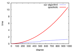
Figure 3: Jacobi polynomials.

Figure 4: Mittag-Leffler polynomials.

Our algorithm performs better than the quadratic one. The crossover points lie between 100 and 200; this large value is due to the constant hidden in our big-Oh estimates: in both cases, there is a contribution of about $20\mathsf{M}(n)$, plus an additional $\mathsf{M}(n)\log(n)$ for Mittag-Leffler.

6 Discussion

This article provides a flexible framework for generating new families of conversion algorithms: it suffices to add new composition operators to Table 1 and provide the corresponding associativity rules. Still, several questions need further investigation. Several of the composition sequences we use are non-trivial: this raises in particular the questions of characterizing what functions can be computed by a composition sequence, and of determining such sequences algorithmically. Besides, the costs of our algorithms are measured only in terms of arithmetic operations; the questions of numerical stability (for floating-point computations) or of coefficient size (when working over $\mathbb{Q}$) require further work.

Acknowledgments. We thank ANR Gecko, the joint Inria-Microsoft Research Lab and NSERC for financial support.

References

- [1] A. V. Aho, K. Steiglitz, and J. D. Ullman. Evaluating polynomials at fixed sets of points. SIAM J. Comp., 4(4):533–539, 1975.
- [2] B. K. Alpert and V. Rokhlin. A fast algorithm for the evaluation of Legendre expansions. SIAM J. Sci. Statist. Comp., 12(1):158–179, 1991.
- [3] G. Andrews, R. Askey, and R. Roy. Special functions. Cambridge University Press, 1999.
- [4] R. Barrio and J. Peña. Basis conversions among univariate polynomial representations. C. R. Math. Acad. Sci. Paris, 339(4):293–298, 2004.
- [5] D. J. Bernstein. Composing power series over a finite ring in essentially linear time. J. Symb. Comp., 26(3):339–341, 1998.
- [6] D. Bini and V. Y. Pan. Polynomial and matrix computations. Vol. 1. Birkhäuser Boston Inc., 1994.
- [7] A. Bostan, G. Lecerf, and É. Schost. Tellegen’s principle into practice. In ISSAC’03, pages 37–44. ACM, 2003.
- [8] A. Bostan, B. Salvy, and É. Schost. Fast algorithms for orthogonal polynomials. In preparation.
- [9] A. Bostan and É. Schost. Polynomial evaluation and interpolation on special sets of points. J. Complexity, 21(4):420–446, 2005.
- [10] R. P. Brent. Multiple-precision zero-finding methods and the complexity of elementary function evaluation. In Analytic Computational Complexity, pages 151–176. Acad. Press, 1975.
- [11] R. P. Brent and H. T. Kung. Fast algorithms for manipulating formal power series. J. ACM, 25(4):581–595, 1978.
- [12] P. Bürgisser, M. Clausen, and A. Shokrollahi. Algebraic complexity theory, volume 315 of GMW. Springer–Verlag, 1997.
- [13] J. Canny, E. Kaltofen, and Y. Lakshman. Solving systems of non-linear polynomial equations faster. In ISSAC’89, pages 121–128. ACM, 1989.
- [14] D. G. Cantor and E. Kaltofen. On fast multiplication of polynomials over arbitrary algebras. Acta Inform., 28(7):693–701, 1991.
- [15] J. R. Driscoll, J. D. M. Healy, and D. N. Rockmore. Fast discrete polynomial transforms with applications to data analysis for distance transitive graphs. SIAM J. Comp., 26(4):1066–1099, 1997.
- [16] M. Frumkin. A fast algorithm for expansion over spherical harmonics. Appl. Algebra Engrg. Comm. Comp., 6(6):333–343, 1995.
- [17] J. g. Gathen and J. Gerhard. Modern computer algebra. Cambridge University Press, 1999.
- [18] J. Gerhard. Modular algorithms for polynomial basis conversion and greatest factorial factorization. In RWCA’00, pages 125–141, 2000.
- [19] G. Hanrot, M. Quercia, and P. Zimmermann. The Middle Product Algorithm, I. Appl. Algebra Engrg. Comm. Comp., 14(6):415–438, 2004.
- [20] G. Hanrot and P. Zimmermann. Newton iteration revisited. http://www.loria.fr/ zimmerma/papers, 2002.
- [21] G. Heinig. Fast and superfast algorithms for Hankel-like matrices related to orthogonal polynomials. In NAA’00, volume 1988 of LNCS, pages 361–380. Springer-Verlag, 2001.
- [22] J. g. Hoeven. Relax, but don’t be too lazy. J. Symb. Comput., 34(6):479–542, 2002.
- [23] E. Kaltofen. Challenges of symbolic computation: my favorite open problems. J. Symb. Comp., 29(6):891–919, 2000.
- [24] E. Kaltofen and Y. Lakshman. Improved sparse multivariate polynomial interpolation algorithms. In ISSAC’88, volume 358 of LNCS, pages 467–474. Springer Verlag, 1989.
- [25] J. Keiner. Computing with expansions in Gegenbauer polynomials. Preprint AMR07/10, U. New South Wales, 2007.
- [26] G. Leibon, D. Rockmore, and G. Chirikjian. A fast Hermite transform with applications to protein structure determination. In SNC’07, pages 117–124, New York, NY, USA, 2007. ACM.
- [27] Y.-M. Li and X.-Y. Zhang. Basis conversion among Bézier, Tchebyshev and Legendre. Comput. Aided Geom. Design, 15(6):637–642, 1998.
- [28] V. Y. Pan. New fast algorithms for polynomial interpolation and evaluation on the Chebyshev node set. Computers and Mathematics with Applications, 35(3):125–129, 1998.
- [29] D. Potts, G. Steidl, and M. Tasche. Fast algorithms for discrete polynomial transforms. Math. Comp., 67(224):1577–1590, 1998.
- [30] S. Roman. The umbral calculus. Dover publications, 2005.
- [31] A. Schönhage and V. Strassen. Schnelle Multiplikation großer Zahlen. Computing, 7:281–292, 1971.
- [32] V. Shoup. A new polynomial factorization algorithm and its implementation. J. Symb. Comp., 20(4):363–397, 1995.