Breakdown of fluctuation-dissipation relations in granular gases

Abstract

A numerical molecular dynamics experiment measuring the two-time correlation function of the transversal velocity field in the homogeneous cooling state of a granular gas is reported. By measuring the decay rate and the amplitude of the correlations, the accuracy of the Landau-Langevin equation of fluctuating hydrodynamics is checked. The results indicate that although a Langevin approach can be valid, the fluctuation-dissipation relation must be modified, since the viscosity parameter appearing in it differs from the usual hydrodynamic shear viscosity .

The hydrodynamic description of ordinary one-component fluids is made by means of the local number density, $n({\bm{r}},t)$, the flow velocity, ${\bm{u}}({\bm{r}},t)$, and the temperature, $T({\bm{r}},t)$ LyL59 . These fields are determined from some closed macroscopic equations, e.g. the Navier-Stokes equations, with the appropriate initial and boundary conditions. On the other hand, the most detailed microscopic description of the evolution of the fluid, in terms of the properties of the particles forming it, is given by non-equilibrium statistical mechanics. In this latter formulation, the hydrodynamic fields appear as the ensemble average of some associated microscopic fields, being also possible to describe their stochastic properties, at least formally. There is an intermediate level of description, often referred to as the mesoscopic description, in which macroscopically fluctuating hydrodynamic fields are considered.

The first formulation of fluctuating hydrodynamics for equilibrium states was proposed by Landau and Lifshitz LyL59 . Their equations describe the fluctuations of the hydrodynamic fields about their equilibrium values, and have the form of linear Langevin equations. The noise terms are taken as white and Gaussian with the second moments determined by the Navier-Stokes transport coefficients of the fluid. This establishes a relationship between the fluctuations of the fields at equilibrium and the dissipation by transport in the fluid, and so are known as fluctuation-dissipation (F-D) relations of the second kind KTyN85 . Since the formulation of the theory, the question of whether the same idea can be used to describe fluctuations in systems that are far away from equilibrium has attracted the attention of scientists. For molecular fluids, it seems well established that the F-D relations apply under the same conditions as the usual Navier-Stokes hydrodynamic equations OyS06 .

Granular fluids are always out of equilibrium due to the kinetic energy dissipation in collisions. Evidence has been accumulated during the last years that they provide a unique proving ground for non-equilibrium statistical mechanics ideas and techniques. Nevertheless, the analogy between granular and ordinary fluids must not be pushed too far. Granular materials have many peculiar properties arising from the macroscopic size of the particles and the lack of kinetic energy conservation before and after a collision JNyB96 . In particular, the validity of the F-D relations can not be assumed a priori.

Here a definite test of the validity of the F-D relations for granular gases is carried out under the most favorable and ideal conditions: the simplest model, state, and hydrodynamic field. If the F-D fails in this case, it will also certainly fail for more “realistic” conditions. More precisely, the behavior of the transversal component of the flow field in the so-called homogeneous cooling state (HCS) of a granular gas is the topic addressed in this paper. Conceptually, this problem is similar to the experimental situation investigated in ref. AMBLyN03 , although the granular state considered is different. To start with, the Landau-Langevin formalism for the transversal velocity field in an equilibrium ordinary fluid will be briefly recalled.

Consider the local fluctuations of the velocity flow $\delta{\bm{u}}({\bm{r}},t)$ around the equilibrium value ${\bm{u}}_{e}={\bm{0}}$, and introduce its Fourier representation $\delta{\bm{u}}_{\bm{q}}(t)$. This vector can be decomposed into the component parallel to ${\bm{q}}$ and another component perpendicular to it: $\delta{\bm{u}}_{\bm{q}}(t)=\delta u_{{\bm{q}},\parallel}\widehat{\bm{q}}+\delta{\bm{u}}_{{\bm{q}},\perp}(t)$, with $\widehat{\bm{q}}\equiv{\bm{q}}/q$ and $\delta{\bm{u}}_{{\bm{q}},\perp}\cdot\widehat{\bm{q}}=0$. The vector component $\delta{\bm{u}}_{{\bm{q}},\perp}(t)$ is the vorticity or transversal flow field and obeys the Langevin equation LyL59

$$\left[\partial_{t}+\left(mn_{e}\right)^{-1}\eta_{e}q^{2}\right]\delta{\bm{u}}_{{\bm{q}},\perp}(t)={\bm{f}}_{{\bm{q}},\perp}(t),$$ (1)

where $m$ is the mass of the fluid particles, $\eta_{e}$ the Navier-Stokes shear viscosity of the fluid, and ${\bm{f}}_{{\bm{q}},\perp}(t)$ a randomly fluctuating force that is a Gaussian white noise of zero average. It verifies the fluctuation-dissipation relation

$$\langle{\bm{f}}_{{\bm{q}},\perp}(t){\bm{f}}_{{\bm{q}}^{\prime},\perp}(t^{\prime})\rangle_{e}=\frac{2T_{e}V}{m^{2}n_{e}^{2}}\,\delta(t-t^{\prime})\delta_{{\bm{q}},-{\bm{q}}^{\prime}}\overline{\eta}_{e}q^{2}{\sf I}.$$ (2)

In the above expressions, angular brackets denote average over the noise realizations, the index e is used to indicate quantities evaluated at equilibrium, $V$ is the volume of the system, ${\sf I}$ is the unit tensor in the subspace perpendicular to ${\bm{q}}$, and $\overline{\eta}_{e}$ a coefficient that according with the Landau theory is the same as the viscosity, $\overline{\eta}_{e}=\eta_{e}$. This is a main physical assertion of the theory.

There is no equilibrium state for granular fluids. Instead, the simplest state for a freely evolving granular fluid is the HCS, mentioned above. At a macroscopic level, it is characterized by a uniform density $n_{H}$, a vanishing flow velocity, and a monotonically decreasing granular temperature, $T_{H}(t)$, that obeys the Haff law Ha83 ,

$$\partial_{t}T_{H}(t)=-\zeta_{H}(T_{H})T_{H}(t),$$ (3)

$\zeta_{H}(T_{H})$ being the cooling rate accounting for the energy dissipation in collisions. The question addressed here is whether Eqs. (1) and (2) are also valid to describe fluctuations of the vorticity in the HCS of a granular fluid as, in fact, has been assumed sometimes in the literature vNEByO97 . Of course, if the answer is negative, there is little hope that those equations hold for stronger non-equilibrium states, such as vibrofluidized granular media.

The simplest and most used model for granular fluids is an ensemble of $N$ smooth inelastic hard spheres ($d=3$) or disks ($d=2$) of diameter $\sigma$ Go03 . Inelasticity is described by means of a constant coefficient of normal restitution $\alpha$, defined in the interval $0<\alpha\leq 1$. For this model, expressions for the transport coefficients have been obtained by using the inelastic Boltzmann-Enskog equation and the Chapman-Enskog procedure. In particular it has been found that BDKyS98 ; GyD99

$$\eta_{H}=mn_{H}\ell_{0}v_{H}(t)\eta^{*}(\alpha,n_{H}),$$ (4)

$$\zeta_{H}(T_{H})=v_{H}(t)\ell_{0}^{-1}\zeta^{*}(\alpha,n_{H}),$$ (5)

where $\ell_{0}\equiv(n_{H}\sigma^{d-1})^{-1}$ is proportional to the mean free path of the particles, $v_{H}(t)\equiv\left[2T_{H}(t)/m\right]^{1/2}$ is a thermal velocity for the HCS, and $\eta^{*}$ and $\zeta^{*}$ are dimensionless functions of the density and the coefficient of restitution. When Eqs. (1) and (2) are applied to the HCS, the problem arises that the viscosity and the second moment of the noise term are time-dependent through the temperature $T_{H}(t)$. It is then convenient to introduce dimensionless length and time scales by ${\bm{\ell}}\equiv{\bm{r}}/\ell_{0}$ and $ds\equiv v_{H}(t)dt/\ell_{0}$, respectively. Moreover, a dimensionless velocity field is defined by ${\bm{\omega}}({\bm{l}},s)\equiv\delta{\bm{u}}({\bm{r}},t)/v_{H}(t)$. Then, Eqs. (1) and (2) become

$$\left(\partial_{s}-\zeta^{*}/2+\eta^{*}k^{2}\right){\bm{\omega}}_{{\bm{k}},\perp}(s)={\bm{\xi}}_{{\bm{k}},\perp}(s),$$ (6)

$$\langle{\bm{\xi}}_{{\bm{k}},\perp}(s){\bm{\xi}}_{{\bm{k}}^{\prime},\perp}(s^{\prime})\rangle_{H}=V^{*2}N^{-1}\delta(s-s^{\prime})\delta_{{\bm{k}},-{\bm{k}}^{\prime}}\overline{\eta}^{*}k^{2}{\sf I},$$ (7)

with ${\bm{k}}=\ell_{0}{\bm{q}}$ and $V^{*}=V/\ell_{o}^{d}$. Moreover, in Eq. (7) it is $\overline{\eta}^{*}=\eta^{*}$. For wavevectors ${\bm{k}}$ such that $\lambda_{\perp}(k)\equiv\zeta^{*}/2-\eta^{*}k^{2}<0$, the long time solution of Eq. (6) reads

$${\bm{\omega}}_{{\bm{k}},\perp}(s)=\int_{-\infty}^{s}ds_{1}\,e^{\lambda_{\perp}(k)(s-s_{1})}{\bm{\xi}}_{{\bm{k}},\perp}(s_{1}).$$ (8)

Using the above expression and Eq. (7), the two-time correlation function of the transverse velocity field is easily obtained,

$${\sf C}_{{\bm{k}},{\bm{k}}^{\prime}}(s,s^{\prime})\equiv\langle{\bm{\omega}}_{{\bm{k}},\perp}(s){\bm{\omega}}_{{\bm{k}}^{\prime},\perp}(s^{\prime})\rangle_{H}=-\frac{V^{*2}\overline{\eta}^{*}k^{2}}{2N\lambda_{\perp}(k)}\,\delta_{{\bm{k}},-{\bm{k}}^{\prime}}e^{\lambda_{\perp}(k)(s-s^{\prime})}{\sf I},$$ (9)

valid for $s\geq s^{\prime}\gg 1$.

In the following, MD simulation results testing Eq. (9) will be reported. Consider a square cell ($d=2$) of side $L$ with periodic boundary conditions, so the minimum value of $k$ allowed is $k_{min}=2\pi\ell_{0}/L$. The value of $L$ has been always chosen such that $k_{min}>k_{\perp}\equiv\left(\zeta^{*}/2\eta^{*}\right)^{1/2}$, to guarantee that the system be always in the parameter region in which it is expected to be stable with respect to vorticity fluctuations, i.e. $\lambda_{\perp}(k_{min})<0$ and Eq. (9) holds for all the allowed values of $k$. In the simulations, fluctuations corresponding to ${\bm{k}}=k_{min}\widehat{\bm{e}}_{x}$, where $\widehat{\bm{e}}_{x}$ is the unit vector in the direction of one of the sides of the cell, have been measured. Therefore, ${\bm{\omega}}_{{\bm{k}},\perp}=\omega_{{\bm{k}},\perp}\widehat{\bm{e}}_{y}$, with $\widehat{\bm{e}}_{y}$ being an unit vector perpendicular to $\widehat{\bm{e}}_{x}$. The particle representation of the transversal velocity field considered here is

$$\delta u_{q_{min}\widehat{\bm{e}}_{x},\perp}(t)=\sum_{i=1}^{N}e^{-2\pi iX_{i}(t)/L}V_{y,i}(t),$$ (10)

where the components of the position and velocity of particle $i$ at time $t$ have been denoted by $X_{i}(t),Y_{i}(t)$ and $V_{x,i}(t),V_{y,i}(t)$, respectively. In the MD simulations an event driven algorithm and the steady state representation of the HCS Lu01 ; BRyM04 have been employed. The fluctuations of the transverse velocity turned out to be always Gaussian within the statistical errors. Moreover, the imaginary part of the two-time correlation function was found to vanish, as expected by symmetry considerations and in agreement with Eq. (9). The restriction to the parameter region in which the HCS is stable implies that the size of the system and, therefore, the number of particles at a given density, is bounded from above. Consequently, relevant size effects show up at low densities. In Fig. 1,

$$\Phi(s,s^{\prime})\equiv\frac{C_{k_{min}\widehat{\bm{e}}_{x},-k_{min}\widehat{\bm{e}}_{x}}(s,s^{\prime})}{C_{k_{min}\widehat{\bm{e}}_{x},-k_{min}\widehat{\bm{e}}_{x}}(s^{\prime},s^{\prime})}$$ (11)

is plotted as a function of $s-s^{\prime}$ for $\alpha=0.8$, $n_{H}\sigma^{2}=0.01$, and several values of $N$, as indicated. In all cases, an exponential decay is observed, in agreement with Eq. (9), that predicts $\Phi(s,s^{\prime})=\exp\left[\lambda_{\perp}(k_{\min})(s-s^{\prime})\right]$. From the data, values for $\lambda_{\perp}(k_{min})$ are obtained. Of course, similar results are found when the labels of the two axis are interchanged. The simulations also provide the value of the cooling rate, that is independent of $N$ and in good agreement with the theoretical prediction given in BDKyS98 ; GyD99 . Then, by subtracting $\zeta^{*}/2$ from the obtained values of $\lambda_{\perp}(k_{min})$, simulation results for the parameter $\eta^{*}$ follow. From the analysis of the data, it follows that the value obtained depends on the number of particles $N$ (size $L$) employed in the simulation. The theoretical prediction corresponds to the formal limit $N\rightarrow\infty$, $L\rightarrow\infty$, with $n_{H}$ constant. In Fig. 2, the values of $\eta^{*}$ obtained from the data in Fig. 1 are plotted as a function of $N^{-1}$. A linear fit leads to the result $\lim_{N\rightarrow\infty}\eta^{*}=(1.059\pm 0.004)\eta^{*}_{e}$, where $\eta^{*}_{e}=(2\sqrt{2\pi})^{-1}$ is the low density (Boltzmann) elastic limit. The theoretical prediction for the Navier-Stokes shear viscosity obtained from the Boltzmann equation in the first Sonine approximation is $\eta^{*}=1.057\eta^{*}_{e}$. Moreover, if a “size-dependent viscosity” is measured by considering the decay of a small macroscopic sine perturbation of the velocity field BRyC99 in systems of different sizes, the values are in good agreement with those reported in Fig. 2. Therefore, it can be concluded that, for the system being investigated, Eq. (9) predicts accurately the decay of the correlation function, with $\eta^{*}$ being the (inelastic) Navier-Stokes shear viscosity.

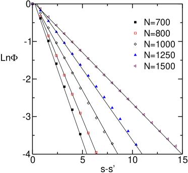
Figure 1: MD simulation results showing the exponential decay of the two-time correlation function of the transversal velocity for $\alpha=0.8$ and $n_{H}\sigma^{2}=0.01$.

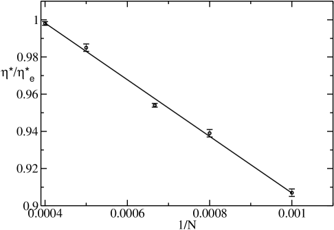
Figure 2: Values of the parameter $\eta^{*}/\eta^{*}_{e}=2\sqrt{2\pi}\eta^{*}$, obtained from the exponential decay of the correlation function of the transversal velocity field, as a function of the inverse of the number of particles $N$. The density and coefficient of restitution are the same as in Fig. 1. Symbols are from MD simulations and the solid line is the best linear fit.

Focus next on the amplitude of the fluctuations. From Eq. (9), it follows that

$$C_{k_{min}\widehat{\bm{e}}_{x},-k_{min}\widehat{\bm{e}}_{x}}(s,s)=-\frac{V^{*2}\overline{\eta}^{*}k_{min}^{2}}{2N\lambda_{\perp}(k_{min})}\,.$$ (12)

Since $\lambda_{\perp}(k_{min})$ was determined from the time decay of the correlation function, the coefficient $\overline{\eta}^{*}$ can be computed from the measurements of the above quantity. Again, a clear dependence on the number of particles $N$ is observed in the results reported in Fig. 3, that correspond to the same system as in Figs. 1 and 2. By means of a linear fit, the asymptotic $N\rightarrow\infty$ value $\overline{\eta}^{*}=1.29\pm 0.02$ is found. It differs from both the shear viscosity of the system measured by the procedures described above and the theoretical prediction in more than $20\%$.

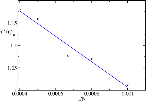
Figure 3: Values of the parameter $\overline{\eta}^{*}/\eta^{*}_{e}=2\sqrt{2\pi}\overline{\eta}^{*}$, obtained from the amplitude of the fluctuations of the transversal velocity field, as a function of the inverse of the number of particles. The density and coefficient of restitution are the same as in Fig. 1. Symbols are from MD simulations and the solid line is the best linear fit.

The above analysis has been repeated for different values of the coefficient of restitution, keeping the density small to allow comparison with the kinetic theory predictions. In particular, the results plotted in Fig. 4 correspond to the case previously discussed and to $\alpha=0.85$, $0.90$, and $0.95$, with $n_{H}\sigma^{2}=6\times 10^{-3}$, $0.018$, and $0.02$, respectively. It is observed that the discrepancy between the shear viscosity $\eta$ and the coefficient $\overline{\eta}$ characterizing the second moment of the fluctuations, increases as the inelasticity increases, vanishing in the elastic limit, as required. In the simulations, attention has been paid to assure that $k_{min}$ is neither too large nor too small. In the former case, the Navier-Stokes approximation is expected to fail, while in the latter instability effects show up.

Two main physical conclusions follow from the study presented here. The Landau-Langevin fluctuating hydrodynamic equations cannot be directly extended to granular fluids. But, on the other hand, it seems possible to separate slow and fast degrees of freedom and to model granular systems in the spirit of the Langevin approach. A similar conclusion was reached from the study of the fluctuations of the total energy of the system BGMyR04 . The open and relevant question is how to express the amplitude of the noise source (i.e. $\overline{\eta}$) in terms of the macroscopic properties of the system. Answering this question requieres to derive Langevin-like equations for the hydrodynamic field of granular fluids stating from kinetic theory or statistical mechanics descriptions.

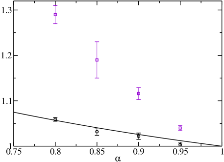
Figure 4: Coefficients $\eta^{*}/\eta^{*}_{e}$ (circles) and $\overline{\eta}^{*}/\eta^{*}_{e}$ (squares) measured from the MD simulations and extrapolated to $N\rightarrow\infty$, as functions of the coefficient of restitution $\alpha$. The density is always very small. The solid line is the Chapman-Enskog prediction in the first Sonine approximation.

This research was supported by the Ministerio de Educación y Ciencia (Spain) through Grant No. FIS2005-01398 (partially financed by FEDER funds). P. Maynar’s work was carried under the HPC-EUROPA project (RII3-CT-2003-506079).

References

- (1) L.D. Landau and E.M. Lifshitz, Fluid Mechanics (Pergamon Press, Oxford 1959).
- (2) R. Kubo, M. Toda, and N. Hashitsume, Statistical Physics II (Springer-Verlag, Berlin, 1985).
- (3) For a recent tutorial review see J.M. Ortiz de Zárate and J.V. Sengers, Hydrodynamic fluctuations (Elsevier, Amsterdam, 2006).
- (4) H.M. Jaeger, S.R. Nagel, and R.P. Behringer, Rev. Mod. Phys. 68, 1259 (1996).
- (5) G. D’Anna, P. Mayor, A. Barrat, V. Loreto, and F. Nori, Nature 424, 909 (2003).
- (6) P.K. Haff, J. Fluid Mech. 134, 401 (1983).
- (7) T.P.C. van Noije, M.H. Ernst, R. Brito, and J.A.G. Orza, Phys. Rev. Lett. 79, 411 (1997).
- (8) I. Goldhirsch, Annu. Rev. Fluid Mech. 35, 267 (2003).
- (9) J.J. Brey, J.W. Dufty, C.S. Kim, and A. Santos, Phys. Rev. E, 58, 4638 (1998).
- (10) V. Garzó and J.W. Dufty, Phys. Rev. E 59, 5895 (1999).
- (11) J.F. Lutsko, Phys. Rev. E 63, 061211 (2001).
- (12) J.J. Brey, M.J. Ruiz-Montero, and F. Moreno, Phys. Rev. E 69, 051303 (2004).
- (13) J.J. Brey, M.J. Ruiz-Montero, and D. Cubero, Europhys. Lett. 48, 359 (1999).
- (14) J.J. Brey, M.I. García de Soria, P. Maynar, and M.J. Ruiz-Montero, Phys. Rev. E 70, 011302 (2004).