Mean-field model for magnetic orders in NpTGa₅ with T=Co, Ni or Rh

Abstract

Characteristics of magnetic transitions in NpTGa₅ with T=Co, Ni, Rh are explained in a unified way with use of a crystalline electric field (CEF) model of localized 5$f^{4}$ electrons. The model takes a CEF doublet and a singlet as local states, and includes dipolar and quadrupolar intersite interactions in the mean-field theory. Diverse ordering phenomena are derived depending on the magnitude of interaction parameters, which qualitatively reproduce the experimentally observed magnetic behaviors in NpTGa₅. The quadrupole degrees of freedom are essential to the diverse magnetic orders. It is argued that NpRhGa₅ is close to a multicritical point where quadrupoles and dipoles with different directions are competing to order.

1 Introduction

Tetragonal $115$ compounds with $4f$ and $5f$ rare earth ions are intensively studied recently because of their intriguing behavior. For example, superconductivity at $T_{c}=18.5$ K has been reported in PuCoGa₅ [1]. The $T_{c}$ is the highest among the heavy-fermion superconductors. The second highest $T_{c}$ has been observed in CeCoIn₅ at 2.3K[2] with the same crystal structure. In heavy fermion systems the superconductivity and magnetism can coexist, and their possible interplay is a longstanding problem. Recently, NpTGa₅ systems with various transition metal ions T attract much attention because of their diverse magnetic behavior. Among these systems, NpCoGa₅ shows an antiferromagnetic (AFM) phase transition at $47$K, which can clearly be seen as a peak in the magnetic susceptibility[3, 4, 5]. It was found by neutron diffraction that the ordered moments are parallel to the tetragonal $c$-axis, and they have the in-plane ferromagnetic structure, while the interplane stacking is antiferromagnetic. Applying magnetic field to this system the ordered phase is suppressed and metamagnetic transition occurs at low temperatures. There are two magnetic transitions in both NpNiGa₅ and NpRhGa₅, but the magnetic structures and the nature of the ordered states are very different in these two systems. The magnetic structure of NpRhGa₅ is the same as that in NpCoGa₅ below the first transition, but with further decrease of temperature the moments switch over to lying within the $ab$-plane by a first order transition[7, 6, 8]. The discontinuous transition is shown as a jump in the magnetic susceptibility and a sharp increase of the magnetic scattering intensities[7]. In NpNiGa₅, a canted AFM structure is found at low temperatures evolving from a ferromagnetically ordered phase of moments lying parallel to the $c$-axis[9]. In this compound both transitions are continuous as indicated by finite jumps in the specific heat. At the lower phase transition a clear anomaly can be seen in the temperature dependence of the total magnetic moment[10]. Perpendicular magnetic order with moments lying within the $ab$-plane is realized in NpFeGa₅ below the Néel temperature 118K. A further weak anomaly was found recently in the thermodynamic quantities such as specific heat and magnetic susceptibility at a lower temperature $\sim 78$K, which indicates a change of the magnetic structure[6]. The presence of magnetic moments at Fe sites makes the behavior more complex in this compound.

In this paper, we explain the mechanism of diverse magnetic orderings of NpTGa₅ systems on the basis of localized picture of 5$f$ electrons. The observed effective magnetic moment in the high-temperature part of the susceptibility in NpCoGa₅ is consistent with the Np³⁺ ($5f^{4}$) configuration, but it highly deviates from the value for Np⁴⁺ ($5f^{3}$) [3]. Furthermore, the magnetic properties of this system above the AFM transition temperature is consistent with a low-lying doublet–singlet crystal field level scheme, where the doublet is the ground state. The next CEF level above this quasi-triplet is lying at about 1200K [3]. Therefore, the low-temperature physics should mainly be determined by the pseudo-triplet states. Due to the layered structure of 115-tetragonal systems, the most important interactions are within the $ab$-planes. We introduce a two-dimensional model by taking the doublet–singlet CEF model within the 5$f^{4}$ configuration to explain the complex properties of NpTGa₅ with T=Co, Ni and Rh. The quadrupole degrees of freedom are found to be essential in understanding the diverse magnetic behavior of NpTGa₅ systems.

This paper is organized as follows. In section 2 we introduce the model Hamiltonian within the pseudo-triplet subspace by clarifying the relevant multipolar interactions. Three different limits of the model are studied in details in section 3, and properties of compounds with T=Co, Rh and Ni are explained in connection with these limits. The summary and discussion is given in the last section.

2 Doublet–singlet CEF model

The Hund’s rule ground state of $5f^{4}$ configuration of Np³⁺ ions is $L=6$ and $S=2$, which gives $J=4$ as the total angular momentum. In tetragonal symmetry the nine-fold degenerate $J=4$ multiplet splits into five singlet and two doublet states. We work in the following doublet-singlet local Hilbert space

$$|d_{\pm}\rangle = a|\pm 3\rangle+\sqrt{1-a^{2}}|\mp 1\rangle$$

$$|s\rangle = c\left(|+4\rangle+|-4\rangle\right)+\sqrt{1-2c^{2}}|0\rangle\,,$$ (1)

which seems to be consistent with the magnetic properties of NpCoGa₅ in the paramagnetic phase[3]. We introduce $\Delta$ as the energy separation between the doublet ground state and the singlet state. The decomposition

$$(E+A_{1})\otimes(E+A_{1})=2A_{1g}\oplus A_{2u}\oplus B_{1g}\oplus B_{2g}\oplus E_{g}\oplus E_{u}$$

shows that the pseudo-triplet space carries the $J_{z}$ ($A_{2u}$) and [$J_{x}$, $J_{y}$] ($E_{u}$) dipoles and $O_{2}^{2}$ ($B_{1g}$), $O_{xy}$ ($B_{2g}$), [$O_{zx}$, $O_{yz}$] ($E_{g}$) quadrupoles as possible local order parameters.

The most important interactions are within a two-dimensional layer including Np ions. For each $ab$-plane, the dipole operators at site $i$ are written as $J_{k,i}$ with $k=x,y,z$, and quadrupole operators as $O_{\mu,i}$ with $\mu=yz,zx,xy$. We consider the nearest-neighbor interactions given by

$${\mathcal{H}}_{ab}=-\frac{1}{4}\sum_{\langle ij\rangle}\left(\sum_{k}\Lambda_{k}J_{k,i}J_{k,j}+\sum_{\mu}\Lambda_{\mu}O_{\mu,i}O_{\mu,j}\right),$$ (2)

where $\langle ij\rangle$ is a nearest-neighbor pair within a tetragonal $ab$–plane. We take the mean-field theory where the factor $1/4$ accounts for the number of nearest-neighbors.

Taking the CEF parameters in basis (1) as $a=0.87$ and $c=0.48$ seems appropriate to describe the high-temperature magnetic properties of NpCoGa₅[3]. In the absence of further information, we use these parameters also in the cases of T=Ni and Rh. With these CEF parameters the eigenvalues of operators $J_{z}$, $J_{x}$, $O_{zx}$ and $O_{xy}$ are derived as $\pm 2.03$, $\pm 1.98$, $\pm 2.35$ and $\pm 2.19$, respectively. Since all the eigenvalues are around $\pm 2$, we normalize the operators $J_{k}$ and $O_{\mu}$ to the same value for simplicity of calculation, and for transparency of the model. Namely, we put their eigenvalues to be $\pm 1,0$ within the pseudo-triplet subspace so that the interaction parameters should roughly be multiplied by 1/4 for the estimate of their magnitude.

The interaction Hamiltonian ${\mathcal{H}}_{ab}$ leads to very complex ordering phenomena even within the pseudo-triplet subspace. We study the following limiting cases of the model. As the simplest limit, we include only $\Lambda_{z}$ and $\Lambda_{xy}$ as the intersite interactions (Case I). Then the singlet excited state and the doublet are decoupled. Next, we introduce nonzero dipole interaction $\Lambda_{x}=\Lambda_{y}$ keeping the quadrupolar interaction $\Lambda_{xy}$ (Case II). Finally, we keep both dipole interactions $\Lambda_{x}=\Lambda_{y}$ and $\Lambda_{z}$, but we assume that the quadrupolar interactions $\Lambda_{zx}=\Lambda_{yz}$ dominate over $\Lambda_{xy}$ (Case III). We argue that these limits are relevant to describe qualitatively the main properties of compounds with Co, Rh and Ni, respectively. Table 1 summarizes the limiting cases. We consider the two-dimensional model given by (2) in Case II and Case III, while only in Case I we additionally introduce Ising-type interlayer coupling in order to calculate also properties in external magnetic field.

Table 1: Limiting cases of the model. Dominant components of dipole and quadrupolar interactions are shown in each case.

	dipole	quadrupole	relevance
Case I	$\Lambda_{z}$	$\Lambda_{xy}$	NpCoGa5
Case II	$\Lambda_{z}$, $\Lambda_{x}=\Lambda_{y}$	$\Lambda_{xy}$	NpRhGa5
Case III	$\Lambda_{z}$, $\Lambda_{x}=\Lambda_{y}$	$\Lambda_{zx}=\Lambda_{yz}$	NpNiGa5

3 Limiting cases of the model

3.1 Case I

As the simplest limit of the model, we first consider only $\Lambda_{z}$ and $\Lambda_{xy}$ setting $\Lambda_{x}=\Lambda_{y}=\Lambda_{zx}=\Lambda_{yz}=0$. Then the singlet excited state is decoupled. The relevant operators in the doublet are represented by the following matrices:

$$J_{z}=\left(\begin{array}[]{cc}1&0\\ 0&-1\end{array}\right),\hskip 14.22636ptO_{xy}=\left(\begin{array}[]{cc}0&-i\\ i&0\end{array}\right).$$ (7)

Thus the doublet can be diagonalized in two different ways leading to Ising-like magnetism ($J_{z}$) or quadrupolar order ($O_{xy}$). The ground state is magnetically ordered with $\langle J_{z}\rangle\neq 0$ for $\Lambda_{z}/\Lambda_{xy}>1$, while for $\Lambda_{z}/\Lambda_{xy}<1$ we get quadrupole-ordered ground state with $\langle O_{xy}\rangle\neq 0$. If we neglect the interlayer interaction, the dipole transition temperature $T_{z}$ is simply given by $T_{z}=\Lambda_{z}$, while the quadrupole transition temperature $T_{Q}$ is given by $T_{Q}=\Lambda_{xy}$.

We argue that the situation in NpCoGa₅, which has a single phase transition at $T_{h\rm N}=47$K, can be described by the doublet limit with $\Lambda_{z}>\Lambda_{xy}$. The energy separation $\Delta\sim 87$K, as estimated as from the high-temperature susceptibility, should be important to the susceptibility anisotropy for example. However, the singlet does not influence the main properties of the model such as the pattern of ordered phases or the nature of the phase transitions.

The AFM ordering in NpCoGa₅ is characterized by the ordering vector ${\bf K}=(0,0,1/2)$ in unit of $(2\pi/a,2\pi/a,2\pi/c)$. In the following, ordering vectors ${\bf k}$ or ${\bf K}$ always mean three-dimensional vectors in unit of $(2\pi/a,2\pi/a,2\pi/c)$, while ordering vectors ${\bf q}$ or ${\bf Q}$ are two-dimensional vectors in unit of $(2\pi/a,2\pi/a)$. To discuss properties in the presence of external magnetic field like magnetic susceptibility or temperature–magnetic field phase diagram, we introduce an interlayer interaction only in the present case as follows:

$${\mathcal{H}}_{c}=\frac{1}{2}\Lambda_{z}^{\perp}\sum_{l}J_{z,i}^{(l)}J_{z,i}^{(l+1)},$$ (8)

where we have explicitly introduced the layer index $l$ in this case, and the factor $1/2$ accounts for the number of nearest neighbors along the $c$ axis. Although the Ising-type interaction has been chosen for simplicity, there is no difference of the result even if we choose an isotropic interlayer interaction. The Ising-type AFM transition temperature $T_{z}$ is given by

$$1-(\Lambda_{z}+\Lambda_{z}^{\perp})\chi_{L}(T_{z})=0,$$ (9)

where we have assumed $\Lambda_{z}^{\perp}>0$, and the local susceptibility $\chi_{L}(T)$ is given by $\chi_{L}(T)=\beta[1+{\rm exp}(-\beta\Delta)/2]^{-1}$ with $\beta=1/T$. The (homogeneous) magnetic susceptibility for $H||(001)$ in the paramagnetic phase ($T>T_{z}$) is given by

$$\chi(T)=\frac{\chi_{L}(T)}{1-(\Lambda_{z}-\Lambda_{z}^{\perp})\chi_{L}(T)}\,.$$ (10)

Note that the antiferromagnetic interplane interaction $\Lambda_{z}^{\perp}>0$ reduces the homogeneous susceptibility.

The left part of Fig. 1 shows the magnetic susceptibility for both magnetic field directions (001) and (100). We use dimensionless coupling constants and magnetic field such as $\lambda_{k,\mu}\equiv\Lambda_{k,\mu}/\Delta$, and $h\equiv g\mu_{\rm B}H/(k_{\rm B}\Delta)$, where $g=3/5$. If we decrease the ratio $\lambda_{z}^{\perp}/\lambda_{z}$, i. e., towards weaker interlayer coupling, the peak in the magnetic susceptibility for $H||(001)$ becomes sharper because of the decrease of the denominator in expression (10).

Figure 1: Left: Temperature dependence of the magnetic susceptibility in the Ising doublet limit. Inset shows the magnetization curves as a function of temperature for fields $h=0.002$, 0.008, 0.017, 0.027 and 0.034. Right: $T$–$H$ phase diagram for field direction $(001)$. Filled squares mean second order transitions, while empty squares represent first order one. We took $\lambda_{z}+\lambda_{z}^{\perp}=0.586$ with $\lambda_{z}^{\perp}/\lambda_{z}=0.05$ in the calculation, which gives the zero field phase transition as $T_{z}/\Delta=0.54$.

We also calculated the temperature dependence of the magnetization, which shows metamagnetic transition at high fields and low temperatures as shown in the inset of Fig. 1. The calculated temperature–magnetic field phase diagram can be seen in the right part of Fig. 1. Let us consider the metamagnetic transition in the ground state. The staggered component of the order parameter $\langle J_{z}\rangle_{A}-\langle J_{z}\rangle_{B}$ vanishes when the magnetic field exceeds a critical value $H_{cr}$. For $H<H_{cr}$ the ground state energy in the mean-field theory can be written as

$${\cal F}_{<}=\frac{1}{4}\lambda_{z}\left(\langle J_{z}\rangle_{A}^{2}+\langle J_{z}\rangle_{B}^{2}\right)-\frac{1}{2}\lambda_{z}^{\perp}\langle J_{z}\rangle_{A}\langle J_{z}\rangle_{B}-\frac{1}{2}(\lambda_{z}+\lambda_{z}^{\perp})\left(\langle J_{z}\rangle_{A}-\langle J_{z}\rangle_{B}\right),$$ (11)

while for $H>H_{cr}$ it becomes

$${\cal F}_{>}=\frac{1}{2}(\lambda_{z}-\lambda_{z}^{\perp})\langle J_{z}\rangle^{2}-(\lambda_{z}-\lambda_{z}^{\perp})\langle J_{z}\rangle-H.$$ (12)

Within the AFM ordered phase the conditions $\partial{\cal F}_{<}/\partial\langle J_{z}\rangle_{A}=0$ and $\partial{\cal F}_{<}/\partial\langle J_{z}\rangle_{B}=0$ gives $\langle J_{z}\rangle_{A}=-\langle J_{z}\rangle_{B}=1$, which leads to ${\cal F}_{<}=-1/2(\lambda_{z}+\lambda_{z}^{\perp})$. Similarly, in the high-field phase we get $\langle J_{z}\rangle=1$ from (12), which gives ${\cal F}_{>}=-1/2(\lambda_{z}-\lambda_{z}^{\perp})-H$. The AFM order vanishes discontinuously by increasing the magnetic field at $H=H_{cr}$, which gives ${\cal F}_{<}={\cal F}_{>}$. From expressions (11) and (12) with $\langle J_{z}\rangle=1$ we get $H_{cr}=\lambda_{z}^{\perp}$. Namely $H_{cr}$ is given by the value of the interlayer coupling constant. This relation clarifies the origin of the metamagnetic transition.

Expression (9) shows that the transition temperature $T_{z}$ is related to the value of $\lambda_{z}+\lambda_{z}^{\perp}$, while the critical magnetic field $H_{\rm cr}$ to $\lambda_{z}^{\perp}$. Therefore, $H_{\rm cr}$ can be small relative to the transition temperature $T_{z}$ if we choose small interlayer coupling $\lambda_{z}^{\perp}$. Furthermore, with small $\lambda_{z}^{\perp}$, the susceptibility is sharply peaked for $H||(001)$. These features are in good agreement with the measured results for NpCoGa₅[3, 4, 5].

3.2 Case II

In this limit we take nonzero dipole interactions $\Lambda_{z}$ and $\Lambda_{x}=\Lambda_{y}$, and assume that the quardupolar interaction $\Lambda_{xy}$ dominates over $\Lambda_{yz}=\Lambda_{zx}$. This $\Lambda_{xy}$ quadrupolar interaction stabilizes the magnetic moment along $(110)$ because of the third order term $\langle J_{x}\rangle\langle J_{y}\rangle\langle O_{xy}\rangle$ in the Landau free-energy expansion. Namely, the system gains the maximum energy when both $\langle J_{x}\rangle$ and $\langle J_{y}\rangle$ are non-zero and equal. The third order term also shows that pure magnetic order of the perpendicular dipoles $\langle J_{x}+J_{y}\rangle$ does not exist, since the quadrupoles $\langle{O}_{xy}\rangle$ are induced by the symmetry.

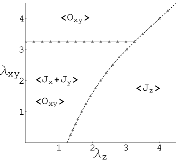
Figure 2: Left: The ground-state phase diagram with $\lambda_{x}=2.13$. For details see the text. Right: Magnetic moment $m=\langle J_{x}+J_{y}\rangle/\sqrt{2}$ in the ground state as a function of $\lambda_{xy}$ for $\lambda_{x}=2.13$ and $\lambda_{z}<1.25$.

The left part of Fig. 2 shows the ground state of the model with fixed $\lambda_{x}=\lambda_{y}=2.13$, which value is chosen as a trial, and $\lambda_{zx}=\lambda_{yz}=0$. In the limit of $\lambda_{xy},\lambda_{z}\gg\lambda_{x}$, the phase boundary between the magnetic ($\langle J_{z}\rangle\neq 0$) and the quadrupolar ($\langle O_{xy}\rangle\neq 0$) phases tends to $\lambda_{z}=\lambda_{xy}$, recovering the doublet limit with $\lambda_{x}=0$. The nonzero $\lambda_{x}$ causes the deviation of the phase boundary from $\lambda_{z}=\lambda_{xy}$ in such a way that the mixed phase with $\langle J_{x}+J_{y}\rangle$$\langle O_{xy}\rangle\neq 0$ expands for $\lambda_{xy}\lesssim\lambda_{x}$ at the expense of phase with $\langle J_{z}\rangle\neq 0$ in the ground state. The right part of Fig. 2 shows the ground state magnetic moment

$$m=\frac{1}{\sqrt{2}}\langle J_{x}+J_{y}\rangle=2\left[\frac{4\lambda_{x}^{2}-1-\lambda_{xy}-2\lambda_{x}\lambda_{xy}}{16\lambda_{x}^{2}-8\lambda_{x}\lambda_{xy}+\lambda_{xy}^{2}}\right]^{1/2}$$ (13)

as a function of the quadrupolar interaction $\lambda_{xy}$ within the mixed phase. We can see that the ordered magnetic moment decreases with increasing quadrupolar interaction, and finally disappears at $\lambda_{xy}=3.26$ in the case of $\lambda_{x}=2.13$. The vanishing of the moment gives the second order phase boundary between the pure quadrupolar phase and the mixed phase. The boundary is given by $\lambda_{xy}=2\lambda_{x}-1$, which can be seen as the horizontal straight line on the phase diagram shown in the left part of Fig. 2.

The compound NpRhGa₅ shows two successive magnetic transitions. From neutron diffraction it is concluded that the magnetic structure below the first transtion $T_{\rm N}^{1}=36$K is the same as that in NpCoGa₅, while at $T_{\rm N}^{2}=33$K the moment changes the direction to $\langle J_{x}+J_{y}\rangle\neq 0$ by a first order transition. The moments are ferromagnetically ordered within each $ab$–plane[7, 6, 8]. The ordered moments $\langle J_{z}\rangle$ completely vanish below 33K. In order to simulate the situation in NpRhGa₅ qualitatively, we now fix a part of parameters as $\lambda_{xy}=1.5$ and $\lambda_{x}=2.13$, and derive the phase diagram in the $\lambda_{z}$–$T$ plane. In the parameter range $\lambda_{xy}\lesssim\lambda_{x}$ the quadrupolar interaction prefers in-plane magnetic moments to the $c$-axis moments. A consequence is that there appears a regime on the $\lambda_{z}$–$T$ phase diagram where an ordered phase with $\langle J_{z}\rangle\neq 0$ undergoes a first order transition to another one with $\langle J_{x}+J_{y}\rangle\langle O_{xy}\rangle\neq 0$ with decreasing temperature. The left part of Fig. 3 shows the calculated phase diagram. Along the path ($\lambda_{z}=1.68$) shown by the arrow, the moment $\mu=\sqrt{(J_{x}+J_{y})^{2}/2+J_{z}^{2}}$ develops as shown in the right panel. The inter-plane AFM coupling $\lambda_{z}^{\perp}$ can simply be included in the mean-field theory by modifying $\lambda_{z}\rightarrow\lambda_{z}+\lambda_{z}^{\perp}$. The magnetic moment increases discontinuously at the first order transition. This behavior is in qualitative agreement with the results found in NpRhGa₅ [7]. Note that with $\lambda_{z}+\lambda_{z}^{\perp}\sim 1.62$, the three phases meet at the multicritical point.

Figure 3: Left: $\lambda_{z}$–$T$ phase diagram for $\lambda_{xy}=1.5$ and $\lambda_{x}=2.13$. Dashed lines indicate the first order transitions, while the solid line represents the second order one. Their meeting point represents a multicritical point which is near the arrow relevant to NpRhGa₅. Right: Temperature dependence of the magnetic moment along the arrow in the upper panel. With $\lambda_{z}+\lambda_{z}^{\perp}=1.68$, the phase transitions are derived as $T_{z}/\Delta=1.31$ and $T_{x}/\Delta=1.36$. Inset shows the moment near the transitions.

We note that the consideration of the singlet state is essential to obtain the perpendicular magnetic order in Case II. This is in contrast to the case of NpCoGa₅, which can be described in the doublet limit. However, the value of the energy separation $\Delta$ is not crucial to the existence of the phases obtained and their characteristic features.

Although we considered a two-dimensional model taking into account only the interactions within the $ab$-planes, we comment shortly on the three-dimensional magnetic and quadrupolar structure. The magnetic moments $\langle J_{x}+J_{y}\rangle$ are ferromagnetically ordered within the $ab$ planes at low temperatures. This means that homogenous quadrupolar moments $\langle O_{xy}\rangle$ are present within the planes even when the quadrupolar coupling constant $\lambda_{xy}$ is zero. The interplane stacking of the magnetic moments is antiferromagnetic, but the ferroquadrupolar order is realized on subsequent planes. This situation is consistent with the invariant term $\langle J_{x}\rangle({\bf k})\langle J_{y}\rangle({\bf-k})\langle O_{xy}\rangle({\bf 0})$ in the Landau free energy expansion. The ferroquadrupolar order means that an orthorombic lattice distortion should develop below $T_{\rm N}^{2}=33$K. We expect experimental observation of the distortion.

3.3 Case III

Now we assume that the quadrupolar interactions $\Lambda_{zx}=\Lambda_{yz}$ dominate over $\Lambda_{xy}$ in contrast with cases of T=Co or Rh. In this case the third order term $\langle J_{z}\rangle(\langle J_{x}\rangle\langle O_{zx}\rangle+\langle J_{y}\rangle\langle O_{yz}\rangle)$ in the Landau expansion plays an important role. Namely, it can lead to two successive transitions both of which are continuous. After the ordering of one of the multipole moments $J_{x}$, $J_{z}$ or $O_{zx}$, a lower phase transition is possible by the simultaneous appearance of the other two multipole moments. A difficulty of the ordinary Landau-type expansion is that the order parameter of the first phase transition is not necessarily small at the second transition, so that the expansion of the free energy with respect to it is not justified. Therefore we use the method developed in ref.kuramoto1, and calculate the Ginzburg-Landau free energy functional in all orders of the finite order parameter which becomes nonzero below the first phase transition. In the present limit we consider the following interactions within the tetragonal $ab$–plane:

$${\mathcal{H}}=-\frac{1}{4}\sum_{\langle ij\rangle}\left(\Lambda_{z}J_{z,i}J_{z,j}+\Lambda_{x}J_{x,i}J_{x,j}+\Lambda_{zx}O_{zx,i}O_{zx,j}\right)\,.$$ (14)

We start with the path-integral representation of the partition function[11]

$${\cal Z}=\int{\cal D}X^{A}{\rm exp}\left[-S_{\rm B}-\int_{0}^{\beta}d\tau{\cal H}(\tau)\right]\,,$$ (15)

where the integration variable $X^{A}$ replaces the operators $J_{x}$, $J_{z}$ and $O_{zx}$. $S_{\rm B}$ is the Berry phase term, which enters because of the non-bosonic commutation property of $J_{x}$, $J_{z}$ and $O_{zx}$. We use the Hubbard-Stratonovich transformation for each imaginary time interval, which is the replacement $-\Lambda_{A}X^{A}\rightarrow\phi^{A}$ by introducing effective fields $\phi^{A}$. These fields $\phi^{A}$ mediate the original interaction. The Hubbard-Stratonovich transformation converts the original inter-site interaction into a local interaction between the effective fields and multipolar operators. Using the property that $\phi$’s have Gaussian distribution, the partition function can be expressed as

$${\cal Z}=\int{\cal D}X^{A}{\cal D}\phi^{A}{\rm exp}\left[-S_{\rm B}-\int_{0}^{\beta}d\tau{\cal H}_{\phi}(\tau)\right]\,,$$ (16)

where

$${\cal H}_{\phi}=\frac{1}{4}\sum_{i,j}\Lambda_{A}\phi_{i}^{A}\phi_{j}^{A}-\frac{1}{2}\sum_{i}\phi_{i}^{A}X_{i}^{A}\,.$$ (17)

We further use the static approximation within which the path integral over $X^{A}$ in ${\cal Z}$ is replaced by trace calculation of corresponding operators[12]. Then we obtain the following form for the partition function

$${\cal Z}=\int{\cal D}\phi^{A}{\rm exp}[-\beta{\cal F}]\,,$$ (18)

where ${\cal F}$ is the Ginzburg-Landau free energy functional given by

$${\cal F} = -N\frac{1}{\beta}{\rm ln}{\cal Z}_{0}+Nf_{\rm mc}$$ (19)

$$+ \frac{1}{4}{\sum_{i,j}}\delta_{ij}\left[\left(\Lambda_{x}^{-1}+d_{1}\right)\phi_{i}^{x}\phi_{j}^{x}+\left(\Lambda_{z}^{-1}+d_{2}\right)\phi_{i}^{z}\phi_{j}^{z}+\left(\Lambda_{zx}^{-1}+d_{1}\right)\phi_{i}^{zx}\phi_{j}^{zx}\right]$$

with

$$d_{1}=\frac{2}{\Delta}\frac{({\rm e}^{-\beta\Delta}-1)}{(2+{\rm e}^{-\beta\Delta})},\hskip 8.5359ptd_{2}=-\beta\frac{2}{(2+{\rm e}^{-\beta\Delta})}\,,$$

and ${\cal Z}_{0}={\rm exp}(-\beta\Delta)+2$. $N$ is the number of the sites. The mode coupling free energy has the form

$$f_{\rm mc}=-\frac{1}{N}\frac{1}{\beta}\sum_{i}\left[{\rm ln}\left({\rm Tr}_{i}{\rm exp}(\beta\phi_{i}^{A}X_{i}^{A}/2)/{\cal Z}_{0}\right)+\frac{1}{4}\beta d_{1}\phi_{i}^{x}\phi_{i}^{x}+\frac{1}{4}\beta d_{1}\phi_{i}^{zx}\phi_{i}^{zx}+\frac{1}{4}\beta d_{2}\phi_{i}^{z}\phi_{i}^{z}\right]\,.$$ (20)

Let us consider the case where the first phase transition at a temperature $T=T_{\rm H}$ corresponds to the ordering of $J_{z}$ dipole moments. This means that for $T<T_{\rm H}$ the expectation value $\langle\phi^{z}_{\bf Q}\rangle=\Lambda_{z}({\bf Q})\langle J_{z}\rangle({\bf Q})$ becomes nonzero, where $\Lambda_{z}({\bf Q})=(1/2)\Lambda_{z}({\rm cos}(Q_{x})+{\rm cos}(Q_{y}))$ is the Fourier transform of the coupling constant $\Lambda_{z}$. The lower transition temperature $T_{\rm L}$ is derived from the condition ${\rm det}(\hat{\chi}^{-1})=0$, where $\hat{\chi}$ is the generalized susceptibility matrix. We have the relation:

$$\hat{\chi}=\hat{J}^{-1}\hat{G}\hat{J}^{-1}-\hat{J}^{-1}\,,$$ (21)

where the interaction matrix $\hat{J}$ is given by

$$\hat{J}=\left(\begin{array}[]{ccc}\Lambda_{z}({\bf Q})&0&0\\ 0&\Lambda_{x}({\bf q})&0\\ 0&0&\Lambda_{zx}(-({\bf q+Q}))\end{array}\right)\,.$$ (25)

The matrix $\hat{G}$ satisfies the following equation [13]

$$\hat{G}=\beta\left(\begin{array}[]{ccc}\langle\phi_{\bf Q}^{z}\phi_{-{\bf Q}}^{z}\rangle&0&0\\ 0&\langle\phi_{\bf q}^{x}\phi_{-{\bf q}}^{x}\rangle&\langle\phi_{\bf q}^{x}\phi_{-({\bf q+Q})}^{zx}\rangle\\ 0&\langle\phi_{-({\bf q+Q})}^{zx}\phi_{\bf q}^{x}\rangle&\langle\phi_{{\bf q+Q}}^{zx}\phi_{-({\bf q+Q})}^{zx}\rangle\end{array}\right)\,,$$ (29)

which means the generalized susceptibility for the effective fields. We are interested in the case where the first transition is ferro-type with ${\bf Q}=0$. Therefore, the wave vector ${\bf q}$ is equivalent to ${\bf q+Q}$.

If the lower transition is also of second order, we make perturbation expansion, under the finite value of $\langle\phi^{z}_{0}\rangle$, for the mode coupling free energy (20) in terms of order parameters $\phi^{x}_{\bf q}$ and $\phi^{zx}_{\bf q}$ up to second order[11]. Then, the Ginzburg-Landau free energy functional can be written in the form

$${\cal F}=\frac{1}{4}H_{11}\phi^{z}_{0}\phi^{z}_{0}+\frac{1}{4}\sum_{i,j=2}^{3}H_{ij}\phi^{i}_{\bf q}\phi^{j}_{-{\bf q}}\,,$$ (30)

where the matrix $\hat{H}=\{H_{ij}\}$ composed by the coefficients of the second order terms is related to $\hat{G}$ as $\hat{H}^{-1}=\hat{G}$, and it has the same block diagonal form. We note when $\phi^{i}$ shows Gaussian distribution, $G^{ij}$ is given by its variance. Using the relation (21) we obtain

$${\rm det}(\hat{\chi}^{-1})=\frac{\Lambda_{z}(0)\Lambda_{x}({\bf q})\Lambda_{zx}({\bf q})H_{11}(H_{22}H_{33}-H_{23}H_{32})}{[\Lambda_{z}(0)^{-1}-H_{11}][(\Lambda_{x}({\bf q})^{-1}-H_{22})(\Lambda_{zx}({\bf q})^{-1}-H_{33})-H_{23}H_{32}]}\,.$$ (31)

Therefore, the condition ${\rm det}(\hat{\chi}^{-1})=0$ is equivalent with ${\rm det}(\hat{H})=0$. Calculating the coefficients $H_{ij}$ in the free energy expansion (30), we can derive the lower phase transition by the condition ${\rm det}(\hat{H})=0$.

• $T\geq T_{\rm H}$
  In this temperature regime with $\langle\phi^{z}_{0}\rangle=0$, the mode coupling free energy (20) gives $H_{23}=H_{32}=0$ in (30). The second order coefficient of term $\phi^{z}_{0}$ can be read from (19) as

  $$H_{11}=\frac{1}{\Lambda_{z}}-\beta\frac{2}{(2+{\rm e}^{-\beta\Delta})}=\frac{1}{\Lambda_{z}}-\chi_{L}\,,$$ (32)

  where we have used that $\Lambda_{z}(0)=\Lambda_{z}$. Due to the block form of matrices $\hat{G}$ and $\hat{H}$, the component of the generalized susceptibility, which corresponds to the dipole operator $J_{z}$ can be obtained as

  $$\chi_{11}=\Lambda_{z}^{-1}(H_{11}^{-1}-1)=\frac{\chi_{L}}{1-\Lambda_{z}\chi_{L}}\,,$$ (33)

  which is the same as expression (10) derived in Case I with $\Lambda_{z}^{\perp}=0$. This is due to the fact that the homogenous magnetic field lying in direction $(001)$ is the conjugated field to the dipole moment $J_{z}$ in the case of ${\bf K}=0$. The first transition temperature $T_{\rm H}$ can be derived from $H_{11}=0$, as the first instability in ordinary Landau mean field theory (see equation (31)). This leads to the condition $1-\Lambda_{z}\chi_{L}(T_{\rm H})=0$, which is the same as expression (9) taking $\Lambda_{z}^{\perp}=0$. Or equivalently, $\chi_{11}^{-1}=0$ leads to the same condition for the transition temperature.

• $T_{\rm H}>T\geq T_{\rm L}$
  In this temperature regime $f_{\rm mc}$ becomes nonzero in the Ginzburg-Landau free energy functional (19). Under the finite value of $\langle\phi^{z}_{0}\rangle=\Lambda_{z}\langle J_{z}\rangle$, the Ginzburg-Landau free energy functional is derived as

  $${\cal F} = \frac{1}{4}\sum_{\bf q}\left[(\Lambda_{x}({\bf q})^{-1}-\pi_{1})\phi_{{\bf q}}^{x}\cdot\phi_{-{\bf q}}^{x}+(\Lambda_{zx}({\bf q})^{-1}-\pi_{1})\phi_{{\bf q}}^{zx}\cdot\phi_{-{\bf q}}^{zx}-\pi_{2}\phi_{{\bf q}}^{x}\cdot\phi_{-{\bf q}}^{zx}\right.$$ (34)

  $$\left.+(\Lambda_{z}^{-1}+d_{2})\phi^{z}_{0}\phi^{z}_{0}-d_{2}\langle\phi^{z}_{0}\rangle^{2}\right]\,,$$

  where

  $$\pi_{1} = \frac{1}{{\tilde{\cal Z}_{0}}}\left(\frac{{\rm e}^{\beta\langle\phi^{z}_{0}\rangle}}{\langle\phi^{z}_{0}\rangle+\Delta}-\frac{{\rm e}^{-\beta\langle\phi^{z}_{0}\rangle}}{\langle\phi^{z}_{0}\rangle-\Delta}+2\Delta\frac{{\rm e}^{-\beta\Delta}}{\langle\phi^{z}_{0}\rangle^{2}-\Delta^{2}}\right)\,,$$

  $$\pi_{2} = \frac{1}{{\tilde{\cal Z}_{0}}}\left(\frac{{\rm e}^{\beta\langle\phi^{z}_{0}\rangle}}{\langle\phi^{z}_{0}\rangle+\Delta}+\frac{{\rm e}^{-\beta\langle\phi^{z}_{0}\rangle}}{\langle\phi^{z}_{0}\rangle-\Delta}-2\langle\phi^{z}_{0}\rangle\frac{{\rm e}^{-\beta\Delta}}{\langle\phi^{z}_{0}\rangle^{2}-\Delta^{2}}\right)\,,$$ (35)

  and ${\tilde{\cal Z}_{0}}={\rm exp}(-\beta\Delta)+2{\rm cosh}(\beta\langle\phi^{z}_{0}\rangle)$. When $\langle\phi^{z}_{0}\rangle\rightarrow 0$ we obtain $\pi_{2}\rightarrow 0$ and $\pi_{1}=-d_{1}$, which means the vanishing of the mixing term as we expect. We then come back to the high temperature form of the GL free energy functional given by (19) with $f_{\rm mc}=0$. The lower transition temperature $T_{\rm L}$ can be derived from ${\rm det}(\hat{\chi}^{-1})=0$ or ${\rm det}(\hat{H})=0$. Explicitly we have the condition

  $$[\Lambda_{x}({\bf q})^{-1}-\pi_{1}(T_{\rm L})][\Lambda_{zx}({\bf q})^{-1}-\pi_{1}(T_{\rm L})]-\pi_{2}(T_{\rm L})^{2}=0\,.$$ (36)

Similar calculation can be performed for the free energy expansion under finite $\langle\phi^{A}_{0}\rangle=\Lambda_{x}(0)\langle J_{x}\rangle(0)$ or $\langle\phi^{A}_{0}\rangle=\Lambda_{zx}(0)\langle O_{zx}\rangle(0)$. The left panel of Fig. 4 shows the ground state ($T=0$) phase diagram with $\lambda_{x}=\Lambda_{x}/\Delta$ fixed at 2.13. We find three regimes where pure dipolar ($J_{z}$ or $J_{x}$) or quadrupolar ($O_{zx}$) order is realized. Thus, we can enter to the regime with mixed order parameters $\langle J_{z}\rangle$–$\langle J_{x}\rangle$–$\langle{O}_{zx}\rangle$ from these three different sides. Let us consider the limiting cases of the phase diagram.
(i) $\lambda_{zx}=0$: there is a first order transition at $\lambda_{z}\approx 1.25$ between the two kinds of magnetic phases. The situation is similar to that in Fig. 2 with $\lambda_{xy}=0$. The phase boundary between the mixed and $\langle J_{z}\rangle\neq 0$ phases can be obtained from condition (36) by taking the limit $T\rightarrow 0$, which gives

$$0 = \left(\frac{1}{\Lambda_{x}}-\frac{1}{\langle\phi^{z}_{0}\rangle+\Delta}\right)\left(\frac{1}{\Lambda_{zx}}-\frac{1}{\langle\phi^{z}_{0}\rangle+\Delta}\right)-\left(\frac{1}{\langle\phi^{z}_{0}\rangle+\Delta}\right)^{2}$$ (37)

$$= \frac{1}{\Delta^{2}}\left(\frac{\lambda_{z}+1-\lambda_{zx}-\lambda_{x}}{\lambda_{x}\lambda_{zx}(\lambda_{z}+1)}\right)\,,$$

where we have used that $\langle\phi^{z}_{0}\rangle=\Lambda_{z}=\lambda_{z}\Delta$ in the ground state. Thus, from (37) the phase boundary is obtained as $\lambda_{zx}=1-\lambda_{x}+\lambda_{z}$. The boundary between the mixed and $\langle J_{x}\rangle\neq 0$ phases is derived as $\lambda_{zx}=\lambda_{x}-\lambda_{z}(1+2\lambda_{x})/(2\lambda_{x}-1)$. The intersection of these two phase boundaries gives the point $\lambda_{z}\approx 1.25$.
(ii) $\lambda_{z}=0$: the point $\lambda_{zx}=2.13\ (=\lambda_{x})$ separates the $\langle J_{x}\rangle\neq 0$ dipolar and $\langle O_{zx}\rangle\neq 0$ quadrupolar phases. The phase boundary between the mixed and $\langle O_{zx}\rangle\neq 0$ phases terminates at

$$\lambda_{zx}=\frac{1}{2}\lambda_{z}+\frac{1}{4}(2\lambda_{x}+1)+\frac{1}{4}\sqrt{(2\lambda_{x}-1)^{2}+4\lambda_{z}^{2}+8\lambda_{z}\lambda_{x}+12\lambda_{z}}.$$

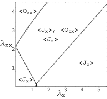
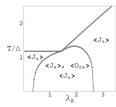
Figure 4: Left: Finite order parameters at $T=0$ in the $\lambda_{z}$–$\lambda_{zx}$ plane with $\lambda_{x}=2.13$. Right: Phase diagram in the $\lambda_{z}$–$T$ plane with a tetracritical point. We have chosen $\lambda_{x}=2.13$ and $\lambda_{zx}=1.5$.

The right panel of Fig. 4 shows the phase diagram in the $\lambda_{z}$–$T$ plane with fixed parameters $\lambda_{x}=2.13$ and $\lambda_{zx}=1.5$. With $\lambda_{z}\gtrsim 1.5$, the first transition makes $\langle J_{z}\rangle\neq 0$, and the second transition gives $\langle J_{x}\rangle\langle{O}_{zx}\rangle\neq 0$ continuously. However for $\lambda_{z}<1.5$, the first transition gives $\langle J_{x}\rangle\neq 0$, and at the lower transition the term $\langle J_{z}\rangle\langle{O}_{zx}\rangle$ becomes nonzero. The transition temperature of the pure $J_{x}$ ordering ($\lambda_{z}<1.5$) is given by

$$T_{x}=-\frac{\Delta}{{\rm ln}(2\lambda_{x}-2)-{\rm ln}(2\lambda_{x}+1)},$$ (38)

which is derived from the vanishing of the coefficient of the second order term $\phi^{x}_{i}\phi^{x}_{j}$ in the free energy expansion (19). The expression (38) leads to the horizontal line $T_{x}/\Delta\approx 1.8$ as a function of $\lambda_{z}$ with $\lambda_{x}=2.13$ (see the phase diagram). The expression (38) also shows that continuous transition to the phase $\langle J_{x}\rangle\neq 0$ is not possible at any temperature with $\lambda_{x}<1$, i. e., $\Lambda_{x}<\Delta$.

The magnetic coupling $\lambda_{z}$ enhances the lower transition temperature by the same mechanism as discussed in ref.libero. The phase diagram contains a tetracritical point at $\lambda_{z}\approx 1.5$, where the four critical lines meet. Phase diagrams with multicritical points should also have experimental interest, because the application of uniaxial pressure or doping can drive the system through a multicritical point to a different regime of the phase diagram with very different physical properties.

We note that the phase diagram presented in the left part of Fig. 4 remains the same for the $(110)$-type perpendicular dipoles instead of the $(100)$-type. Namely, there is a continuous degeneracy with respect to the phase transition temperature within the $J_{x}$–$J_{y}$ order parameter space due to the tetragonal symmetry. The difference is that the ordered quadrupoles will have nonzero moments $\langle O_{zx}+O_{yz}\rangle$ instead of $\langle O_{zx}\rangle\neq 0$.

In NpNiGa₅ there appear two successive continuous phase transitions at $T_{\rm c}=30$K and $T_{\rm N}=18$K [9, 6]. The first one is the ferromagnetic ordering of $J_{z}$ dipoles with the ordering vector ${\bf K}=(0,0,0)$. At temperature $T_{\rm N}$ non-zero $\langle J_{x}\rangle$ component appears with ${\bf k}=(1/2,1/2,1/2)$, leading to a canted antiferromagnetic structure. In ref.honda two possibilities are mentioned for the orderings: (i) both transitions correspond to the Np sublattice or (ii) one of the transitions related to the Ni sublattice. We assume that both transitions are caused by the Np ions, which is consistent with recent neutron diffraction results[4].

Figure 5: Left: Temperature dependence of the specific heat with two transitions at $T_{z}/\Delta\approx 15$ and $T_{c}/\Delta\approx 13.6$. The parameters are chosen as $\lambda_{x}=\lambda_{zx}=16.5$ and $\lambda_{z}=22$. Right: Temperature dependence of $\theta$ (degree) and the moment $\mu$.

In order to investigate the second transition to an ordered phase with $\langle J_{z}\rangle\neq 0$, we take the simplifying limit $\lambda_{x}=\lambda_{zx}$. Then the free energy can be calculated by the diagonalization of the Hamiltonian within the basis (1). The left panel of Fig.5 shows the specific heat against temperature with two second-order transitions. We also calculated the direction of the spontaneous moment ($\theta$) below the lower transition temperature and the total magnetic moment ($\mu$) as a function of temperature (see right part of Fig.5). We define the spontaneous moment $\overrightarrow{\mu}=\langle J_{x}\rangle\hat{x}+\langle J_{z}\rangle\hat{z}$, and its deviation from the direction $\hat{z}$ as ${\rm tan}(\theta/2)=\langle J_{x}\rangle/\langle J_{z}\rangle$. The magnitude of the moment is given by $\mu=\sqrt{\langle J_{x}\rangle^{2}+\langle J_{z}\rangle^{2}}$. The calculated temperature dependences of $\theta$ and $\mu$ are shown in the right panel of Fig. 5. The lower transition causes an anomaly in $\mu$ in good correspondence with the experimental result in NpNiGa₅[10].

In the case of antiferromagnetic coupling $\lambda_{x}<0$, the lower quadrupolar transition will lead to a canted AFM structure within the $ab$-planes. In order to have the non-zero invariant term $\langle J_{x}\rangle({\bf Q}_{x})\langle O_{zx}\rangle({\bf Q}_{zx})\langle J_{z}\rangle({\bf Q}_{z})$ with the ordering wave vectors in the parenthesis, the condition ${\bf Q}_{zx}=-({\bf Q}_{x}+{\bf Q}_{z})=-{\bf Q}_{x}$ should be satisfied with ${\bf Q}_{z}=0$. Hence the quadrupolar order should have the same ordering vector ${\bf Q}_{x}=(1/2,1/2)$ as that of $J_{x}$.

4 Summary and Discussion

In this work we have studied a two-dimensional mean field model composed of a non-Kramers doublet ground state and a singlet excited state. The model includes dipolar and quadrupolar degrees of freedom. The layered structure of $f$ ions should be important in realizing characteristic magnetism and superconductivity in $115$ systems. For theoretical consideration of these systems, a relevant picture should be a strong two-dimensional interaction and a weak interlayer interaction. Therefore, the main interactions which determine the magnetic structure are within the two-dimensional $ab$-planes. The main purpose of this work is to understand the origin of the complex magnetic structures of NpTGa₅ systems with T=Co, Ni and Rh. Thus, we have studied a two-dimensional model which includes interactions within the tetragonal $ab$-planes. We have analyzed some limiting cases of the model by changing the interaction parameters, and found behaviors reminiscent of the magnetic properties of NpTGa₅ systems with T=Co, Ni and Rh.

The intersite interactions in NpTGa₅ with T=Ni may be different from those with T=Co or Rh since the Fermi surface of NpNiGa₅ contains one more conduction electrons per unit cell. The difference in the number of $d$-electrons may be a reason why in NpNiGa₅ the quadrupolar interactions $\lambda_{zx}=\lambda_{yz}$ dominate over $\lambda_{xy}$ in contrast with cases of T=Co, Rh. On the other hand, the CEF structure should be less sensitive to the change of the Fermi surface. It is likely that other Np 115 systems may correspond to a shifted parameter space. Then multicritical behaviors can be expected under appropriate conditions. For example, the ordering of the perpendicular magnetic moments can also happen first depending on the interaction parameters. The perpendicular moments experimentally found in NpPtGa₅[15] seem to be explained in this way.

It is always a question in the case of actinide compounds whether the electrons are localized or itinerant. There is a tendency of increasing localization with increasing atomic number along the $f$ series of the elements in the periodic table. The element Np, situated between U and Pu, seems to be at the localized-itinerant border. Recent NMR results on NpCoGa₅ suggest localized behavior in contrast to the more itinerant-like UCoGa₅[16]. Among the Np compounds, NpO₂ is an example where the localized description works well to describe the triple-q octupolar order below $25$K. Even in the case of U-based compounds, the localized picture may apply to the case of the famous hidden ordered phase of URu₂Si₂. Although our simple CEF model can explain the diverse behavior realized in NpTGa₅, the purely localized model cannot explain the enhanced $T$-linear term in the specific heat, for example. Hence a more sophisticated model is desirable to account for the dual character of $5f$ electrons. We note that in the case of even number of $5f$ electrons as in Np³⁺, electronic states in the localized limit and the band limit may be connected continuously [17].

A further question is the value of the ordered magnetic moments at low temperatures. It is found experimentally that in the case of NpCoGa₅ the saturated magnetic moment is about $0.84\mu_{\rm B}$/Np, and it is $0.96\mu_{\rm B}$/Np in NpRhGa₅. In the mean field theory, the zero temperature value of the moments is mainly determined by the crystal field parameters. For example, with crystal field parameter $a=0.87$ we get $1.22\mu_{\rm B}$ for the saturated magnetic moment $J_{z}$ in the case of NpCoGa₅, which is larger than the observed value. We saw previously in the case of NpRhGa₅ that the presence of quadrupolar interaction $\lambda_{xy}$ can reduce the value of the magnetic moment $\langle J_{x}+J_{y}\rangle$. On the other hand, quantum fluctuations can lead to the reduction of the ordered moment even for localized electrons. We expect stronger fluctuations in the Np $115$ systems because of the strong two-dimensional feature compared to the case of the cubic NpGa₃, for example, in which the ordered moments are about $1.51\mu_{\rm B}$[18].

The main properties of NpTGa₅ systems with T=Co, Ni and Rh can be understood within the two-dimensional model. However, in order to discuss behavior in the presence of magnetic field like susceptibility anisotropy, for example, the interlayer coupling should be also included. Only in the case of NpCoGa₅ we have included an interlayer interaction, and calculated properties in external magnetic field. It would be interesting to incorporate interlayer coupling also in the cases of T=Ni and Rh and compare the obtained results to the measured ones. The difference in the number of conduction electrons may be a reason why the interlayer RKKY coupling becomes ferromagnetic in NpNiGa5, as compared with observed antiferromagnetic interlayer ordering in NpCoGa₅ and NpRhGa₅ We plan to discuss these issues in a subsequent work.

References

- [1] J. L. Sarrao, L. A. Morales, J. D. Thompson, B. L. Scott, G. R. Stewart, F. Wastin, J. Rebizant, P. Boulet, E. Colineau and G. H. Lander: Nature 420 (2002) 297.
- [2] C. Petrovich, P. G. Pagliuso, M. F. Hundley, R. Movshovich, J. L. Sarrao, J. D. Thompson, Z. Fisk and P. Monthoux: J. Phys.: Condensed Matter 13 (2001) L337.
- [3] D. Aoki, Y. Homma, Y. Shiokawa, E. Yamamoto, A. Nakamura, Y. Haga, R. Settai, T. Takeuchi and Y. nuki: J. Phys. Soc. Jpn. 73 (2004) 1665.
- [4] N. Metoki, K. Kaneko, E. Colineau, P. Javorský, D. Aoki, Y. Homma, P. Boulet, F. Wastin, Y. Shiokawa, N. Bernhoeft, E. Yamamoto, Y. nuki, J. Rebizant and G. H. Lander: Phys. Rev. B 72 (2005) 014460.
- [5] E. Colineau, P. Javorský, P. Boulet, F. Wastin, J. C. Griveau, J. Rebizant, J. P. Sanchez and G. R. Stewart: Phys. Rev. B 69 (2004) 184411.
- [6] D. Aoki et al, Y. Homma, Y. Shiokawa, H. Sakai, E. Yamamoto, A. Nakamura, Y. Haga, R. Settai and Y. nuki: J. Phys. Soc. Jpn. 74 (2005) 2323.
- [7] S. Jonen et al., submitted to PRB.
- [8] E. Colineau, F. Wastin, P. Boulet, P. Javorský, J. Rebizant and J. P. Sanchez: J. Alloys and Compounds 386 (2005) 57.
- [9] F. Honda, N. Metoki, K. Kaneko, D. Aoki, Y. Homma, E. Yamamoto, Y. Shiokawa, Y. nuki, E. Colineau, N. Bernhoeft and G. H. Lander: Physica B 359-361 (2005) 1147.
- [10] F. Honda et al., to be published.
- [11] H. Kusunose and Y. Kuramoto, J. Phys. Soc. Jpn. 70 (2001) 1751.
- [12] Y. Kuramoto and N. Fukushima, J. Phys. Soc. Jpn. 67 (2000) 583.
- [13] Y. Kuramoto and H. Kusunose, J. Phys. Soc. Jpn. 69 (2000) 671.
- [14] V. L. Libero and D. L. Cox, Phys. Rev. B 48 (1993) 3783.
- [15] F. Honda et al., to be published.
- [16] S. Kambe et al., to be published.
- [17] S. Watanabe, Y. Kuramoto, T. Nishino and N. Shibata, J. Phys. Soc. Jpn. 68 (1999) 159.
- [18] M. N. Bouillet, T. Charvolin, A. Blaise, P. Burlet, J. M. Fournier, J. Larroque and J. P. Sanchez: J. Magn. Magn. Mater. 125 (1993) 113.