Red Galaxy Growth and the Halo Occupation Distribution
Abstract
We have traced the past of red galaxy stellar mass growth within dark matter halos. We have determined the halo occupation distribution, which describes how galaxies reside within dark matter halos, using the observed luminosity function and clustering of 40,696 red galaxies in Boötes. Half of halos host a red central galaxy, and this fraction increases with increasing halo mass. We do not observe any evolution of the relationship between red galaxy stellar mass and host halo mass, although we expect both galaxy stellar masses and halo masses to evolve over cosmic time. We find that the stellar mass contained within the red population has doubled since , with the stellar mass within red satellite galaxies tripling over this redshift range. In cluster mass halos () most of the stellar mass resides within satellite galaxies and the intra-cluster light, with a minority of the stellar mass residing within central galaxies. The stellar masses of the most luminous red central galaxies are proportional to halo mass to the power of . We thus conclude that halo mergers do not always lead to rapid growth of central galaxies. While very massive halos often double in mass over the past , the stellar masses of their central galaxies typically grow by only .
1 INTRODUCTION
In a universe where the bulk of the mass is in the form of collisionless cold dark matter (CDM), galaxies reside within gravitationally bound halos of CDM particles (White & Rees 1978). The motion of these particles is effectively governed by gravity alone, so both the mass function and clustering of dark matter halos are predictable, albeit non-trivial, functions of redshift and cosmological parameters (e.g., Press & Schechter 1974; Sheth & Tormen 1999; Jenkins et al. 2001; White 2002; Tinker et al. 2005). Gravitational collapse results in the growth of dark matter halos over cosmic time while dynamical friction leads to the orbital decay and merging of substructure within halos. As a consequence, there is the expectation that the galaxies residing within these halos will also grow via mergers.
In a CDM cosmology, halos more massive than groups () undergo rapid growth via merging between and the present day. If the stellar mass within every dark matter halo was always contained within a single central galaxy, we would expect the most massive galaxies to undergo rapid growth via mergers at . Until relatively recently, the rapid growth of massive galaxies at was an almost universal prediction of CDM galaxy formation models (e.g., White & Frenk 1991; De Lucia et al. 2006). However, it is difficult to predict the rate at which substructure merges within halos (e.g., Taylor & Babul 2001; Benson et al. 2003; Taffoni et al. 2003; Boylan-Kolchin, Ma, & Quataert 2008) and at least some simulations overestimate the rate of galaxy growth via mergers.
As much of the stellar mass within groups and clusters resides within satellites (e.g., Sandage, Binggeli, & Tammann 1985; Lin & Mohr 2004) and the diffuse intra-cluster light (ICL; e.g., Kemp & Meaburn 1991; Gonzalez et al. 2000; Arnaboldi et al. 2002; Feldmeier et al. 2004; Zibetti et al. 2005), not all halo mergers funnel stellar mass directly into central galaxies. It is thus plausible that massive galaxies do not grow as rapidly as their host halos. The current generation of CDM galaxy formation models predict a range of assembly histories for massive galaxies, with rates of stellar mass growth varying by up to a factor of 2 (e.g., Baugh et al. 2005; Bower et al. 2006; De Lucia et al. 2006; Naab et al. 2007). When plausible models produce widely varying predictions, there is a clear need for robust observations to test these predictions.
There is compelling observational evidence that galaxies grow via mergers at . There are thousands of examples of merging galaxies in the literature, spanning a broad range of galaxy types, mass and redshift (e.g., Arp & Madore 1987; Toomre & Toomre 1972; Conselice et al. 2003; van Dokkum 2005; Rines, Finn, & Vikhlinin 2007; McIntosh et al. 2007; Lotz et al. 2008). While there have been valiant attempts to measure the rate of galaxy growth using catalogs of merging galaxies or galaxy pairs, there are large uncertainties associated with the selection function of such objects and the time-scales for merging. At low redshift, measured rates of red galaxy stellar mass growth via mergers span from per (e.g., Masjedi et al. 2006; Masjedi, Hogg, & Blanton 2007) to per (e.g., van Dokkum 2005). Although the exact merger rate remains a matter of debate, clearly there is some assembly of red galaxies via merging at .
The evolving space density of galaxies is a conceptually simple method for measuring the growth of galaxy stellar masses. At the epoch where the most massive galaxies are assembled, their space density will increase with decreasing redshift. Although conceptually simple, in practice such measurements are difficult. Very luminous galaxies are strongly clustered (e.g., Norberg et al. 2002; Zehavi et al. 2005a), so uncertainties are dominated by the sample variance from large-scale structure rather than Poisson counting statistics. The most massive galaxies typically possess strong 4000 Å breaks and lack strong emission lines, which complicates both optical photometry and spectroscopy of galaxies. Despite these difficulties, there is increasing evidence that the stellar masses of the most massive galaxies grow by 50% or less at (e.g., Bundy et al. 2006; Cimatti, Daddi, & Renzini 2006; Wake et al. 2006; Brown et al. 2007; Scarlata et al. 2007). As a consequence, pure passive evolution models without any mergers remain popular (e.g., Cimatti et al. 2006; Wake et al. 2006; Scarlata et al. 2007), as they provide a better approximation of massive galaxy evolution than many simulations using CDM cosmologies. However, since there is compelling evidence for galaxy mergers, the rate of stellar mass growth must be non-zero.
Measurements of the relationship between galaxy stellar mass and dark matter halo mass provide important clues as to how galaxies grow over cosmic time. For example, if galaxy stellar mass was directly proportional to host halo mass we would expect galaxies to grow as rapidly as their host dark matter halos during mergers. The relationship between galaxy stellar mass and halo mass has been explored, using various methods for estimating halo mass, including gravitational lensing (e.g., Hoekstra, Yee, & Gladders 2004; Mandelbaum et al. 2006b), satellite galaxy velocities (e.g., Conroy et al. 2007b), X-ray temperature (e.g., Lin & Mohr 2004), X-ray luminosity (e.g., Brough et al. 2008), group velocity dispersion (e.g., Brough et al. 2006), galaxy clustering (e.g., van den Bosch, Yang, & Mo 2003; Zheng, Coil, & Zehavi 2007) and matching the galaxy luminosity function with the predicted halo mass function (e.g., Vale & Ostriker 2004). For the most massive galaxies, these studies find that galaxy stellar mass scales as halo mass to the power of roughly a third.
The halo occupation distribution (HOD; e.g., Peacock & Smith 2000; Seljak 2000; Berlind & Weinberg 2002; Cooray & Sheth 2002) describes the number and distribution of galaxies within dark matter halos. As the clustering and space density of dark matter halos are predictable functions of redshift, HOD models can be constrained with the observed clustering and space density of galaxies. HOD models combine much of the relevant astrophysics (e.g., the halo mass function) with empirical descriptions of how galaxies reside within dark matter halos. While such models cannot be considered complete descriptions of galaxy evolution, they do provide key insights into how galaxies grow over cosmic time. For example, if halo mergers efficiently funnel stellar mass into central galaxies, we would expect relatively little stellar mass to reside within satellite galaxies.
In this paper, we determine the HOD using the measurements of the luminosity function and clustering of red galaxies selected from the Boötes field of the NOAO Deep Wide-Field Survey (NDWFS) and Spitzer IRAC Shallow Survey. This work builds upon our previous study of the HOD of the most massive () red galaxies in Boötes (White et al. 2007, see §5.3 for a summary). Red galaxies are an ideal population for measuring the HOD and testing the predictions of galaxy formation models. As red galaxies have low star-formation rates, the growth of individual galaxies at should be dominated by merging (via dynamical friction) rather than star-formation, thus simplifying the comparison of CDM models and data. In CDM models the most massive halos undergo rapid growth via mergers at , and if this results in rapid growth of central galaxies, then this should be observable within our sample. The spectral energy distributions of red galaxies are dominated by old stellar populations, so the optical luminosities of red galaxies are tightly correlated with stellar mass. Although our halo masses rely upon CDM models of the space density and clustering of halos, we can compare our halo masses with those derived with other techniques (e.g., X-ray temperature, weak lensing). In several galaxy formation models virial shock heating (e.g., Birnboim & Dekel 2003; Dekel & Birnboim 2006; Khochfar & Ostriker 2007) or feedback from Active Galactic Nuclei (AGNs; e.g., Silk & Rees 1998; Wyithe & Loeb 2003; Croton et al. 2006; Hopkins et al. 2006) truncates star-formation in halos above a critical mass, and this mass scale should be observable with a well constrained HOD.
The structure of this paper is as follows. In §2 we describe the NDWFS and IRAC Shallow Survey, the object catalogs and our red galaxy sample. We present measurements of the evolving luminosity function and luminosity density of red galaxies in §3. In §4 we discuss the correlation function of red galaxies as a function of both luminosity and redshift, including comparisons with the literature. We discuss the HOD modeling of the clustering and space density of red galaxies in §5, including a discussion of the evolving relationship between galaxy luminosity and halo mass. In §6 we introduce an illustrative analytic model of the red galaxy HOD, and discuss how stellar mass evolves within the central and satellite red galaxy populations. We summarize our key results in §7. Appendix A provides an overview of the analytic method used to determine preliminary angular correlation function covariance matrices. Appendix B describes the mock galaxy catalogs, which we used to determine the uncertainties of the luminosity function and our final estimates of the correlation function covariance matrices.
Throughout this paper we use Vega magnitudes and a flat cosmology with , , , and . Our choice of cosmology is similar to the WMAP-3 cosmology (Spergel et al. 2007) and matches the dark matter simulation we used to generate mock galaxy catalogs. For the analytic calculation of the HOD (§5), we define halos as spherical objects where the mean density within the sphere is 200 times that of the background. For the mock catalogs, halos are identified using a Friends-of-Friends algorithm which is discussed in detail in Appendix B. We denote base ten logarithms with and natural logarithms with .
2 IMAGING, CATALOGS AND THE RED GALAXY SAMPLE
We selected our red galaxy sample from imaging of the Boötes field by NDWFS and IRAC Shallow Survey. Our sample is extremely similar to that of Brown et al. (2007), and we refer the reader to that paper for a more thorough description of the surveys, source detection, photometry, photometric redshifts, rest-frame properties, catalog completeness and sanity checks. The only significant difference between this work and Brown et al. (2007) is that we adopt a flat cosmology with and rather than and . This cosmology matches that of the dark matter simulation we use to generate mock galaxy catalogs (Appendix B) and is similar to the WMAP-3 cosmology (Spergel et al. 2007).
2.1 IMAGING
In this paper we utilize optical and infrared imaging of Boötes from the NDWFS (Jannuzi & Dey 1999) and Spitzer IRAC Shallow Survey (Eisenhardt et al. 2004). The NDWFS is an optical () and near-infrared () imaging survey of two fields with telescopes of the National Optical Astronomy Observatory. We utilize the third NDWFS data release111Available from the NOAO Science Archive at http://www.archive.noao.edu/ndwfs/ of optical imaging with the MOSAIC-I camera on the Kitt Peak 4-m telescope. To obtain accurate optical colors with fixed aperture photometry across the Boötes field, we have smoothed copies of the released images to a common Point Spread Function (PSF) with a full width at half maximum of . The IRAC Shallow Survey is of contiguous imaging with the Infrared Array Camera (IRAC; Fazio et al. 2004) of Spitzer Space Telescope. The Boötes field was imaged at wavelengths of , , , and with a typical exposure time of . We utilize the and imaging to remove contaminants (e.g., stars) from our galaxy sample and (when combined with the NDWFS photometry) for photometric redshifts .
2.2 SOURCE DETECTION AND PHOTOMETRY
We detected sources using SExtractor (Bertin & Arnouts 1996), run on the -band images of the NDWFS third data release. For this paper, we only include objects which are detected within nominal subfield boundaries. The subfields have small overlaps and we remove duplicate object detections from these regions. To minimize contamination of the catalog, we exclude regions surrounding very extended galaxies and saturated stars. Regions without good coverage from both the NDWFS and the IRAC Shallow Survey are also excluded. The final sample area is over a field-of-view.
We measured aperture photometry for each object using our own code. SExtractor segmentation maps were used to exclude flux associated with neighboring objects. We corrected the photometry for missing pixels (e.g., bad pixels) using the mean flux per pixel measured in a series of annuli surrounding each object. Uncertainties were determined by measuring photometry at positions within of the object position and finding the uncertainty which encompassed 68% of the measurements. The accuracy of the photometry was verified by adding artificial galaxies to our data, recovering them with SExtractor and measuring their photometry with our code (Brown et al. 2007).
2.3 PHOTOMETRIC REDSHIFTS
We determined redshifts for our galaxies using the empirical ANNz photometric redshift code (Firth, Lahav, & Somerville 2003; Collister & Lahav 2004). ANNz uses artificial neural networks to determine the relationship between measured galaxy properties and redshift. It does not use any prior assumptions about the shape of galaxy spectral energy distributions (SEDs), though it does assume the relationship between observed galaxy properties and redshift is a relatively smooth function.
The basis of our training set is galaxies with spectroscopic redshifts in Boötes. The AGN and Galaxy Evolution Survey (AGES, C. S. Kochanek et al. in preparation) has obtained spectroscopic redshifts of galaxies, while several hundred additional redshifts are available from a variety of programs with 4 and 8 m-class telescopes. At and there are relatively few galaxies with spectroscopic redshifts, so we added artificial galaxies to the training set by (at fixed redshift) interpolating in color and extrapolating in luminosity. We trained and measured photometric redshifts using the aperture photometry and the 2nd order moments of the -band light distribution. Using 4319 red galaxies with spectroscopic redshifts, we find the uncertainties of our photometric redshifts are in redshift at , decreasing to at .
2.4 REST-FRAME PROPERTIES
To measure absolute magnitudes and rest-frame colors, we used maximum likelihood fits of Bruzual & Charlot (2003) SED models to the optical photometry. Throughout this paper we use solar metallicity models with a Salpeter (1955) initial mass function, a formation redshift of , and a broad range of exponentially declining star formation rates. As with all SED models and templates, these models do have errors but these have little impact upon our principal conclusions (Brown et al. 2007, §6.5).
The aperture photometry captures 86% or less of the total flux. We corrected for the flux outside this aperture by assuming galaxies within our sample have de Vaucouleurs (1948) profiles truncated at 7 half-light radii. We adopt the same size-luminosity relation as Brown et al. (2007) and assume this relation undergoes luminosity evolution described by a Bruzual & Charlot (2003) stellar synthesis model with a formation redshift of . While the size-luminosity relation of red galaxies has some scatter, this should have little impact upon our results as aperture photometry captures most of the flux from red galaxies (see Figure 5 of Brown et al. 2007).
2.5 THE RED GALAXY SAMPLE
The distribution of galaxy colors is bimodal (e.g., Hogg et al. 2004), and selection criteria for red galaxies typically fall near the minimum between the red and blue galaxy populations (e.g., Madgwick et al. 2002; Bell et al. 2004; Willmer et al. 2006). We apply a similar approach here, and use the following rest-frame color selection criterion:
| (1) | |||||
Our criterion selects galaxies with rest-frame colors within magnitudes of the evolving color-magnitude relation of red galaxies. This criterion allows comparison with the recent literature and is similar to the criterion of Bell et al. (2004). We also applied apparent color cuts to remove contaminants while not significantly reducing sample completeness, and these are discussed in detail in Brown et al. (2007).
The completeness of the catalogs was verified by adding artificial galaxies with de Vaucouleurs (1948) profiles to copies of our data and recovering them with SExtractor. Our catalogs are more than 85% complete for galaxies with half-light radii of or less. We limit the absolute magnitude range in each of our redshift bins so we can determine accurate redshifts and have a sample completeness of 85% or more. Our final sample contains 40,696 red galaxies with photometric redshifts between and .
3 THE RED GALAXY LUMINOSITY FUNCTION
Our red galaxy sample is very similar to that of Brown et al. (2007), except we adopt a slightly different flat cosmology with and . This increases the luminosity distance by 3% and the comoving volume by 10%. We select our sample using absolute magnitude criteria, so our sample size is 4% larger than that of Brown et al. (2007). While these changes are small, they are comparable to our random uncertainties, so we present revised measurements of the red galaxy luminosity function and luminosity density here.
Our methodology for measuring the luminosity function is very similar to that of Brown et al. (2007). We measure the evolving luminosity function of red galaxies using both the binned estimator (Schmidt 1968) and maximum-likelihood fits of Schechter (1976) luminosity functions. Our photometric redshift errors are relatively small and their impact upon the measured luminosity functions is estimated to be negligible (Brown et al. 2007). We split the sample into four photometric redshift slices: , , and , which have comoving volumes of , , and respectively. The total comoving volume of is comparable to that of the 2dF Galaxy Redshift Survey (2dFGRS).
Unlike Brown et al. (2007), we estimate the uncertainties for the luminosity function using multiple mock galaxy catalogs, whose construction is described in Appendix B. We expect the uncertainties derived from mock catalogs to be more robust than those determined with subsamples of the data, as individual large-scale structures can span multiple subsamples. Fractional uncertainties derived from mocks are on the order of 10%, and can be 50% larger than those determined with subsamples.
To quantify the evolution of stellar mass within the red population, we measure the luminosity density (the luminosity weighted integral of the luminosity function). To determine the -band luminosity density () we sum over the galaxy catalog () at each redshift bin, apply corrections for sample incompleteness, and divide by the volume of the relevant redshift slice. Galaxies fainter than our magnitude limits contribute up to of the luminosity density, and we include their contribution using an analytic approximation of the HOD (§6). Our measurements of the luminosity function and luminosity density are summarized in Tables 1 and 2.
The overall evolution of the luminosity function is very similar to that reported by Brown et al. (2007) and our principal conclusions remain unchanged. The luminosity density decreases by only between and , while the -band luminosity of an aging stellar population fades by a factor of 3 over the same redshift range. We thus conclude that the stellar mass within the red galaxy population has increased by since . Mergers of red galaxies (without accompanying star-formation) do not increase the stellar mass contained within the red population. As there is little star-formation within the red population, the increase in stellar mass must result from stellar mass being transferred from the blue galaxy population to the red galaxy population (e.g., Bell et al. 2004; Brown et al. 2007; Faber et al. 2007).
The transfer of stellar mass from the blue galaxy population into the red galaxy population will have little impact on the space density of the most luminous red galaxies unless significant merging takes place, as very massive blue galaxies are rare at (e.g., Bell et al. 2004). The evolving space density of luminous red galaxies thus provides strong constraints on the rate of galaxy stellar mass growth via galaxy mergers. The bright end () of the red galaxy luminosity function fades by -band magnitudes between and . We would not expect to see any fading if massive galaxies were being rapidly assembled via mergers at . However, the bright end of the luminosity function does not fade by the -band magnitudes predicted by passive stellar population synthesis models (e.g., Bruzual & Charlot 2003) and the luminosity evolution of the fundamental plane (e.g., van Dokkum & Stanford 2003; Treu et al. 2005). We thus conclude that there is ongoing assembly of massive galaxies at , albeit at a rate that only increases their stellar masses by between and .
4 MEASURING THE RED GALAXY CORRELATION FUNCTION
The spatial correlation function of galaxies is one of the principal constraints on the HOD. In particular, the clustering of galaxies on scales less than is a strong function of the number of satellite galaxies residing within halos. We measured the clustering of red galaxies with the angular correlation function, and then used the Limber (1954) equation to compare models of the spatial clustering with our observations. Angular correlation functions were determined using subsamples of red galaxies selected as a function of photometric redshift, luminosity and space density. A summary of the subsample properties, including galaxy counts and photometric redshift ranges, is provided in Table 3.
4.1 THE ANGULAR CORRELATION FUNCTION
We measured the angular correlation function with the Landy & Szalay (1993) estimator:
| (2) |
where , , and are the number of galaxy-galaxy, galaxy-random and random-random pairs at angular separation . The pair counts were determined in bins spaced by between and .
For a field of finite size, estimators of the correlation function are subject to the integral constraint where
| (3) |
(Groth & Peebles 1977), where is the angle separating solid angle elements and . The integral constraint results in a systematic underestimate of the true clustering. If the number density fluctuations in the volume are small, and the angular correlations are smaller than the variance within the volume, then to first order the correlation function is simply biased low by a constant equal to the fractional variance of the number counts. Often, to remove this bias, the term
| (4) |
is added to where is the survey area. The value of , where is an estimate of the mean number of galaxies per unit area, is the contribution of clustering to the variance of the galaxy number counts (Groth & Peebles 1977; Efstathiou et al. 1991).
Our final estimates of the integral constraint use the variance of the galaxy number counts measured from multiple mock galaxy catalogs (Appendix B). Before constructing the mock catalogs, preliminary estimates of the integral constraint were derived from power-law fits to the angular correlation function. The integral constraint depends on the value of on large angular scales. On such scales, the angular correlation function of mock catalog galaxies is constrained by the clustering of dark matter halos while power-law extrapolations of the correlation function are strongly dependent on the measured value of the power-law index. Both mock catalogs and power-law fits (where the power-law index of the spatial correlation function is ) provide comparable estimates of the integral constraint, with . The significance of the integral constraint reaches a maximum of for the largest angular scales of our highest redshift bins. On the angular scales where most of our constraining power comes from, the integral constraint is negligible.
4.2 THE COVARIANCE MATRIX
To fit a functional form to the measured angular correlation function, we need a model covariance matrix to estimate uncertainties of our data points and the correlations between them. Commonly used methods for estimating the covariance matrix include mock catalogs, subsampling or resampling of the data, and analytic approximations.
For our preliminary measurements, we estimated covariance matrices using the analytic approximations described in Appendix A. Analytic covariance matrices can be computed quickly and do not include random noise, but can have large systematic errors. The final results presented in this paper use covariance matrices determined with mock catalogs, whose construction we discuss in Appendix B. The mock covariance matrices naturally include the effects of sample variance and shot-noise without making assumptions about the linearity of the underlying clustering or special relations of higher order functions. The mock catalogs are generated using a dark matter simulation and an analytic approximation of how red galaxies reside within dark matter halos (§6). The analytic approximation of the HOD was initially constrained with angular correlation functions determined with the analytic covariance matrices, and was then verified using mock catalog covariance matrices.
4.3 THE GALAXY REDSHIFT DISTRIBUTION
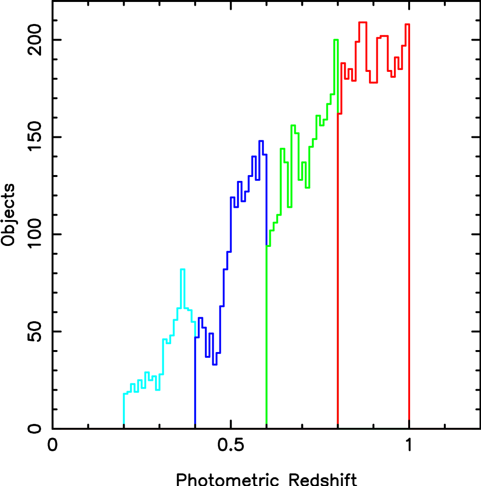
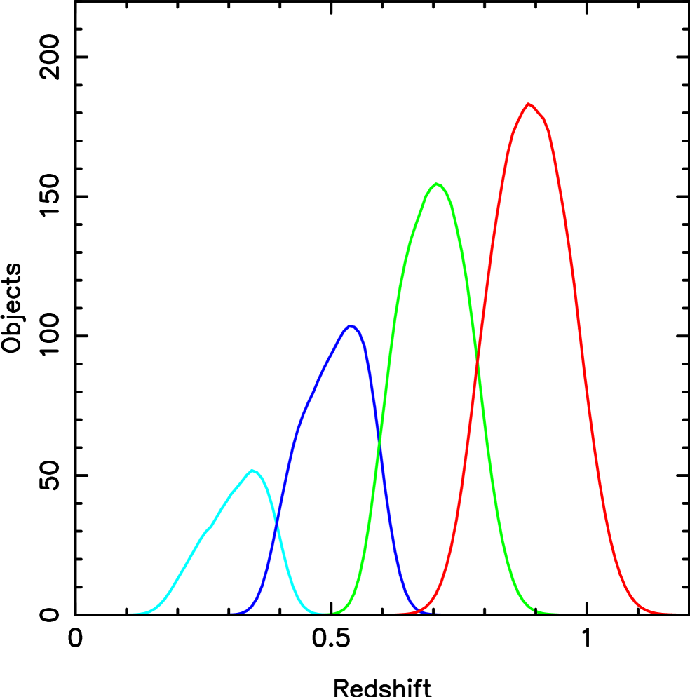
The angular correlation function, , can be derived from the spatial correlation function , using the Limber (1954) equation:
| (5) | |||||
where is the spectroscopic redshift distribution, and is the comoving distance between two objects at redshifts and separated by angle on the sky. If the functional form of the spatial correlation function is known, the spatial correlation function can be determined with accurate measurements of the angular clustering and a robust model of the galaxy redshift distribution.
To model the redshift distributions of our subsamples, we use the Schechter luminosity functions listed in Table 2. Photometric redshift uncertainties result in objects being scattered into and out of our subsamples. To model this, we use the measured photometric redshift uncertainties from Table 4 of Brown et al. (2007), which are a function of both galaxy magnitude and redshift, and assume Gaussian random errors. We have not attempted to model gross photometric redshift errors as they are rare in our sample (see Figure 3 of Brown et al. 2007). If we did not include these uncertainties, we would underestimate the mean physical separation of galaxy pairs and underestimate by approximately 20%. The photometric redshift and model spectroscopic redshift distributions for four of our red galaxy samples are shown in Figure 1. As the spectroscopic redshift distribution of neighboring photometric redshift bins overlap, neighboring bins are not completely independent of each other.
Our model redshift distributions are a function of the measured photometric redshift uncertainties. As a consequence, if our photometric redshift uncertainties are in error our measurement of will also be in error. To verify this is not the case, we checked that our estimate of did not depend on the width of our redshift bins (Brown et al. 2003). When a redshift bin is very narrow, the width of the model redshift distribution is dominated by the photometric redshift uncertainties. Conversely, the model redshift distribution for a very wide redshift bin has relatively little dependence on the photometric redshift uncertainties. We found that our clustering estimates did not vary when we modified the width of our redshift bins, consistent with there being no gross errors in our model redshift distributions.
4.4 POWER-LAW MODELS OF THE CORRELATION FUNCTION
Power-laws provide a simple empirical approximation of the spatial correlation function, enabling quick comparison with the literature. Also, unlike the HOD, power-law models of the correlation function do not depend on models of the space density and clustering of dark matter halos. However, spatial correlation functions measured with large redshift surveys do show significant departures from power-laws (e.g., Zehavi et al. 2004; Zheng et al. 2007). Also, power-laws are a purely empirical description of the galaxy clustering and are not physically motivated. Power-law approximations of the correlation function are thus useful but should be treated with due caution.
We approximate the spatial correlation function with the standard power-law parameterization:
| (6) |
where is the galaxy pair separation in comoving coordinates and is the spatial scale where . As a consequence, the angular correlation function is also parameterized by a power-law:
| (7) |
We use rather than to parameterize the strength of the angular clustering, as the measured value strongly depends on the measured value .
We plot examples of power-law fits to the angular correlation function in Figures 2 and 3, along with HOD model fits (see §5) for comparison. While HOD models provide better fits to spatial correlation functions measured with large redshift surveys (e.g., Zehavi et al. 2004; Zheng et al. 2007), we find comparable values for HOD model and power-law fits to our data. This is not altogether surprising, as our sample is much smaller than comparable SDSS samples and (for a given sample) angular correlation functions have lower signal-to-noise than spatial correlation functions.
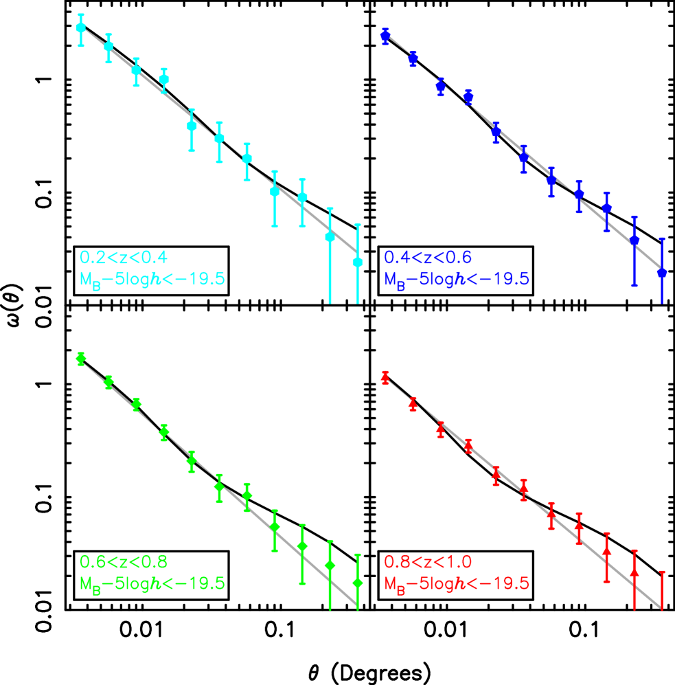
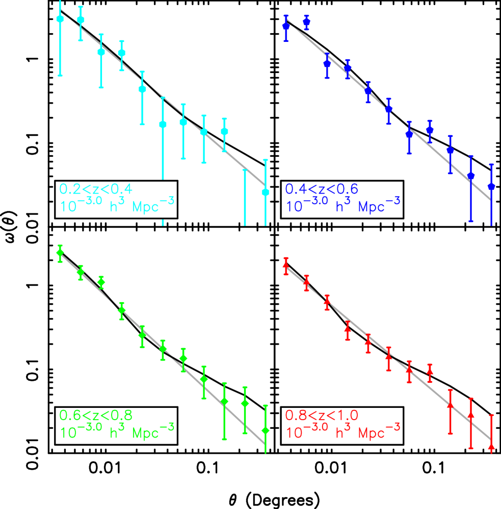
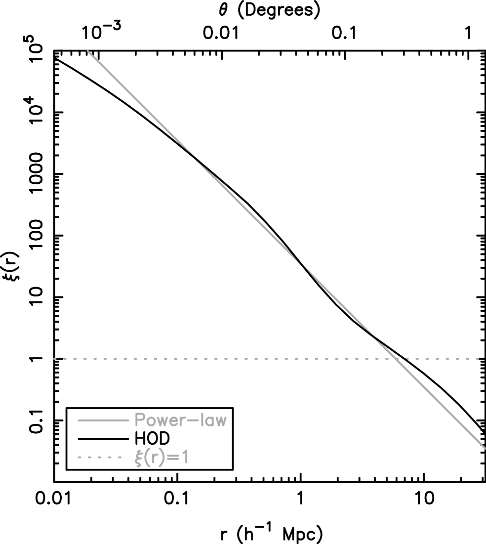
We determined the value of for each subsample using the measured values of and , models of the galaxy redshift distribution and the Limber (1954) equation. We provide a complete list of our power-law correlation function parameters in Table 3. We best constrain the spatial correlation function on scales of , and on scales larger than our power-law models should be considered extrapolations. As we show in Figure 4, the scale where power-law and HOD models of equal unity often differ by , so one should treat values from this work and the literature with caution.
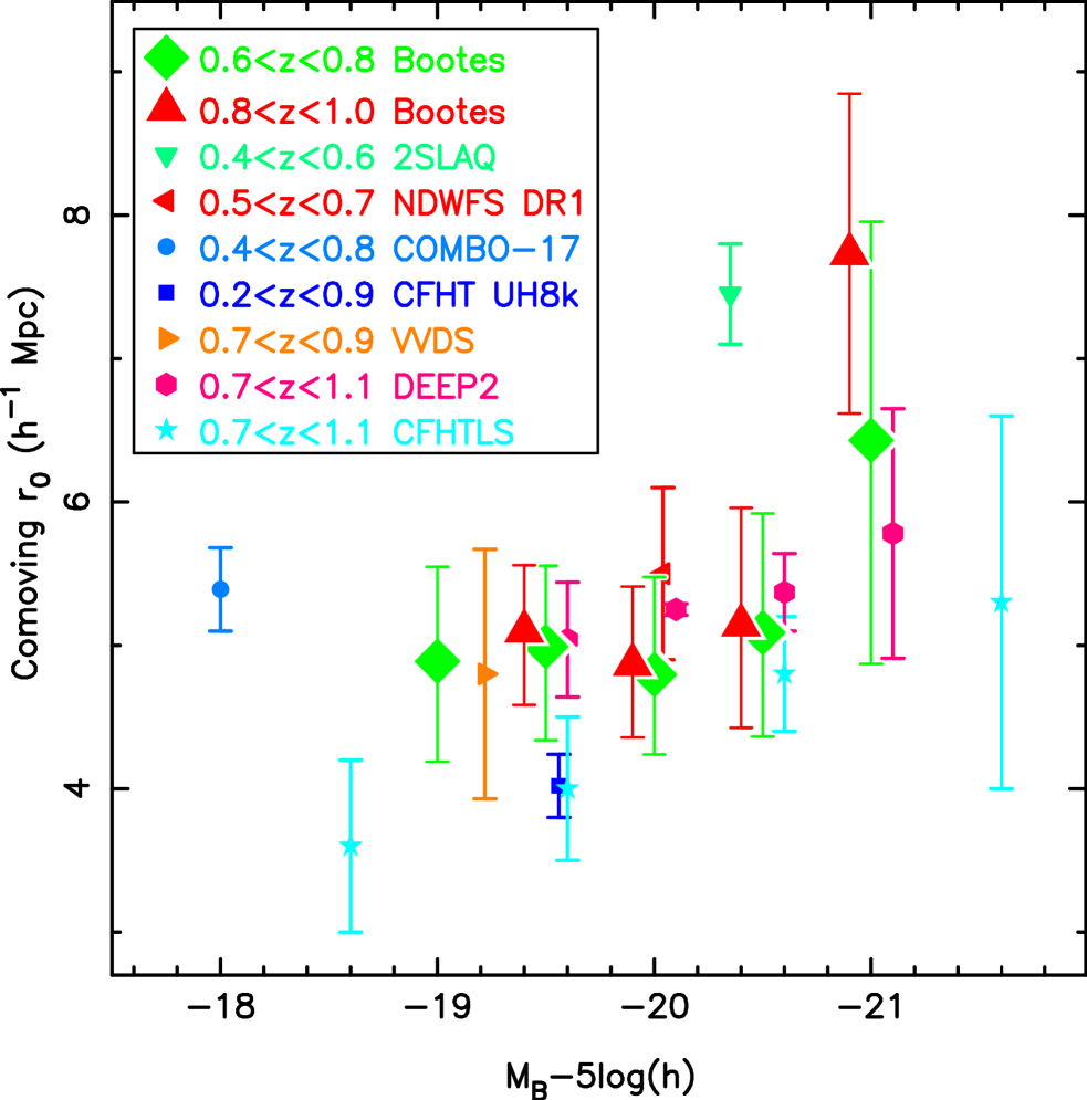
In Figure 5 we plot the spatial clustering of red galaxies in Boötes (parameterized by ) along with results from the recent literature at comparable redshifts (Brown et al. 2003; Wilson 2003; Meneux et al. 2006; Phleps et al. 2006; McCracken et al. 2007; Ross et al. 2007; Coil et al. 2008). Measurements from the CFHT UH8k survey (Wilson 2003) and the CFHT Legacy Survey (McCracken et al. 2007) are systematically low, as their model redshift distributions do not account for photometric redshift errors. The clustering of red galaxies fainter than is roughly constant as a function of both luminosity and redshift, with . There is some evidence that the spatial clustering of luminous red galaxies is correlated with luminosity at high redshift, as one would expect if the most massive galaxies reside within the most massive (and strongly clustered) dark matter halos. As halo masses are a product of HOD modeling, we will return to this point later in the paper.
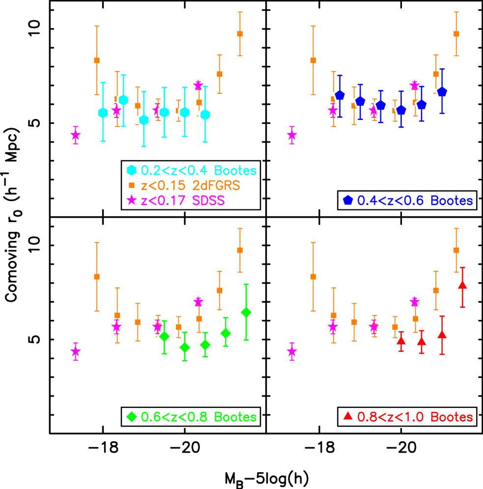
The clustering of red galaxies in Boötes, as a function of both luminosity and redshift, is plotted in Figure 6. For comparison we also plot low redshift measurements from the 2dFGRS (Norberg et al. 2002) and SDSS (Zehavi et al. 2005b). We have used the model S0 colors of Fukugita, Shimasaku, & Ichikawa (1995) to include the 2dFGRS and SDSS measurements in Figure 6. We find that the clustering of red galaxies is clearly a strong function of luminosity for galaxies brighter than . This trend disappears or weakens for fainter galaxies. The faintest SDSS data-point suggests the correlation of with luminosity continues to fainter magnitudes, but the power-law approximation of this subsample has an unusually high value of (2.46) which may explain the unusually low estimate of . The clustering of red galaxies as a function of luminosity clearly evolves with redshift. However, as we expect aging stellar populations to fade by 1.2 -band magnitudes between and , much of this evolution is due to luminosity evolution rather than the evolution of large-scale structure.
5 HALO OCCUPATION DISTRIBUTION MODELING
Halo occupation distribution (HOD; e.g., Peacock & Smith 2000; Seljak 2000; Berlind & Weinberg 2002; Cooray & Sheth 2002) modeling is a powerful tool for understanding the clustering of galaxies and how galaxies reside within dark matter halos. The principle of the HOD framework is to link galaxies to their host dark matter halos, whose formation and properties can be predicted by both simulations and analytic methods. As the evolving space density and clustering of dark matter halos are predictable functions of redshift, one can determine the galaxy HOD with the observed space density and clustering of galaxies. By measuring the HOD as a function of both galaxy luminosity and redshift, one obtains the evolving relationship between galaxy luminosity and host halo mass. One can thus determine how galaxy stellar masses are growing with respect to the masses of the dark matter halos in which the galaxies reside.
5.1 HOD MODELING OF THE CORRELATION FUNCTION
The conceptually simplest method of implementing HOD modeling is to populate halos identified in cosmological -body simulations. We use this approach to generate mock galaxy catalogs, which we discuss in detail in Appendix B. The simulation provides halo masses and positions, while the HOD specifies the mean number and spatial distribution of galaxies within halos.
The functional form of the HOD is typically motivated by the results of galaxy formation models, and it is physically reasonable to split the HOD into central and satellite galaxy components (e.g., Kravtsov et al. 2004; Zheng et al. 2005). By definition central galaxies are found at the center of halos and there is only zero or one central galaxy per halo (although the mean number of centrals per halo can lie between zero and one). Multiple satellite galaxies can reside within a halo, and their spatial distribution is often assumed to follow the dark matter distribution.
Once a set of HOD parameter values has been chosen, one can step through the halo catalog and populate each halo with galaxies. The HOD provides the probabilities that a halo will contain a central galaxy and a particular number of satellites. One can thus determine the number of galaxies in a given halo using these probabilities and a random number generator. The HOD also provides the probability of a satellite being at a particular radius from the halo center, so a random number generator can be used to assign satellite positions within halos. Once a catalog is populated with galaxies, one can mimic the observations and statistics used to measure the properties of the galaxy population (in this case, the luminosity and angular correlation functions). One can repeat the process, exploring a range of HOD parameter values, until a best-fit model is found.
While it is conceptually simple to populate a simulated halo catalog, it is computationally expensive. Analytic methods of HOD modeling have been developed which allow quick computation of the galaxy space density and clustering statistics (HOD; e.g., Peacock & Smith 2000; Seljak 2000; Berlind & Weinberg 2002; Cooray & Sheth 2002). These methods use descriptions of halo properties which have been calibrated against -body simulations. We employ an analytic methodology which is extremely similar to that of White et al. (2007) and Zheng et al. (2007). We utilize analytic approximations for the halo mass function (Jenkins et al. 2001), the biased clustering of halos (Tinker et al. 2005), the profile of dark matter within halos (NFW; Navarro, Frenk, & White 1996), the concentration of halo profiles (Bullock et al. 2001) and the non-linear dark matter power-spectrum (Smith et al. 2003). The galaxy space density is the integral of the halo mass function multiplied by the mean number of galaxies per halo. In the analytic calculation, the two-point correlation function is the sum of two terms, the one-halo term and the two-halo term.
The one-halo term results from pairs of galaxies which reside within the same halo (intra-halo pairs). This term is dominant on small scales and, by definition, is sensitive to the fraction of galaxies which are satellites. Given an HOD model, the one-halo term is just the distribution of intra-halo galaxy pair separations as a function of halo mass convolved with the halo mass function. The calculation of this term is usually decomposed into contributions by central-satellite and satellite-satellite pairs. We assume satellite galaxies follow the dark matter distribution within halos, which we model with NFW profiles. As a result, the spatial distribution of central-satellite pairs follows an NFW profile while that of satellite-satellite pairs follows an NFW profile convolved with itself.
The two-halo term results from pairs of galaxies which reside within different halos, and this term dominates the correlation function on large scales. On the largest scales it is equal to the mass correlation function times the mean galaxy-weighted halo bias squared. On scales smaller than one must include prescriptions for halo exclusion (halos cannot reside within each other) and scale-dependent bias. In practice it is easier to calculate the power spectrum of the two-halo term rather than directly calculate the spatial correlation function, and we refer interested readers to Zheng (2004) and Tinker et al. (2005) for further details.
5.2 HOD PARAMETERIZATION
We use a five parameter model to describe the mean number of central and satellite galaxies (brighter than some luminosity) per halo. We plot an example of this model in Figure 7 and discuss the model in detail below. The functional form of this model is motivated by HODs observed in galaxy formation simulations (Berlind et al. 2003; Kravtsov et al. 2004; Zheng et al. 2005). The mean number of central galaxies per halo is modeled with
| (8) |
where erf is the error function
| (9) |
At a halo mass of , 50% of halos host a central galaxy. If the relationship between galaxy luminosity and halo mass had no scatter, would be modeled by a step function. In reality this relation must have some scatter, resulting in a gradual transition from to , whose width we quantify with the parameter .
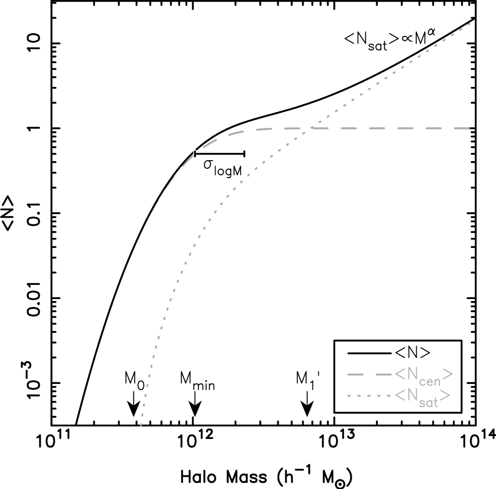
We approximate the mean number of satellite galaxies per halo with a power-law truncated at a threshold mass of :
| (10) |
The parameter corresponds to the halo mass where when (as is the case here) and . When and , the mean number of satellites per halo is proportional to halo mass. The number of satellites in halos of a given mass is assumed to follow a Poisson distribution, which is consistent with theoretical predictions (Kravtsov et al. 2004; Zheng et al. 2005) and current observational constraints (Yang et al. 2005; Ho et al. 2007; Yang, Mo, & van den Bosch 2007).
For each subsample of the red galaxy catalog we tested a range of plausible HOD models. For each HOD model we determined the galaxy space density and spatial correlation function using the analytic methodology described above, and then determined the corresponding angular correlation function using the Limber (1954) equation. For each HOD model we estimated values using the full covariance matrices and a space density prior including fractional uncertainties determined using mock catalogs.
To rapidly explore the plausible range of HOD parameter space we applied the Markov Chain Monte Carlo method (MCMC; e.g., see Gilks, Richardson, & Spiegelhalter 1996). This method generates a list (or chain) of HOD parameters whose frequency in the chain traces the likelihood of that model fitting the data. It works by generating random HODs from a trial distribution and accepting or rejecting them based on the relative likelihood of the fit. We choose new models by perturbing the HOD parameters from the last accepted chain element by Gaussian offsets in the log of the relevant parameter. The step size and directions are determined from the covariance matrix of a previous run of the chain. We further restricted the HOD parameter space to those models with . Each chain provides the HOD distribution and a set of models which provide good fits to the observations.
We provide a summary of our best-fit HOD parameter values in Tables 4 and 5. While and have small uncertainties, the other parameters are poorly constrained. As the measured HOD parameter values are correlated with each other, and as a function of luminosity would show less scatter if the other HOD parameters had well determined values. For this reason, in Table 5 we provide fits of HOD models where only and are free parameters while the other parameters are fixed at , and . The fixed parameters have values that are similar to those in Table 4 and the predictions of simulations (e.g., Zheng et al. 2005; Seo, Eisenstein, & Zehavi 2007).
5.3 THE RED GALAXY HOD
Models of the correlation function derived from the HOD provide a robust estimate of the large-scale bias factor, (where ), which we plot as a function of absolute magnitude in Figure 8. HOD models better constrain the bias factor than power-law extrapolations, which depend on the measured value of and result in a varying bias factor on large scales. The bias factor increases with redshift, as the spatial clustering of red galaxies evolves slowly while the underlying dark matter distribution evolves rapidly. As noted previously, the bias (or clustering strength) is a strong function of luminosity for the brightest red galaxies while varying little for galaxies fainter than .
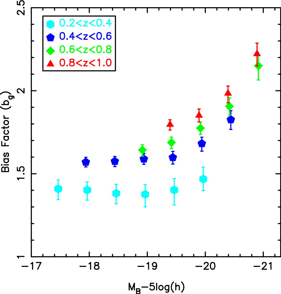
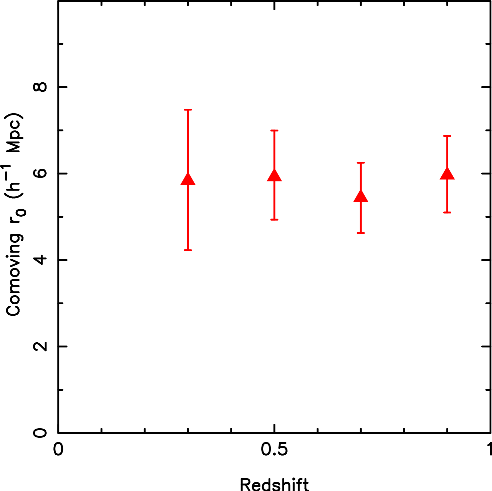
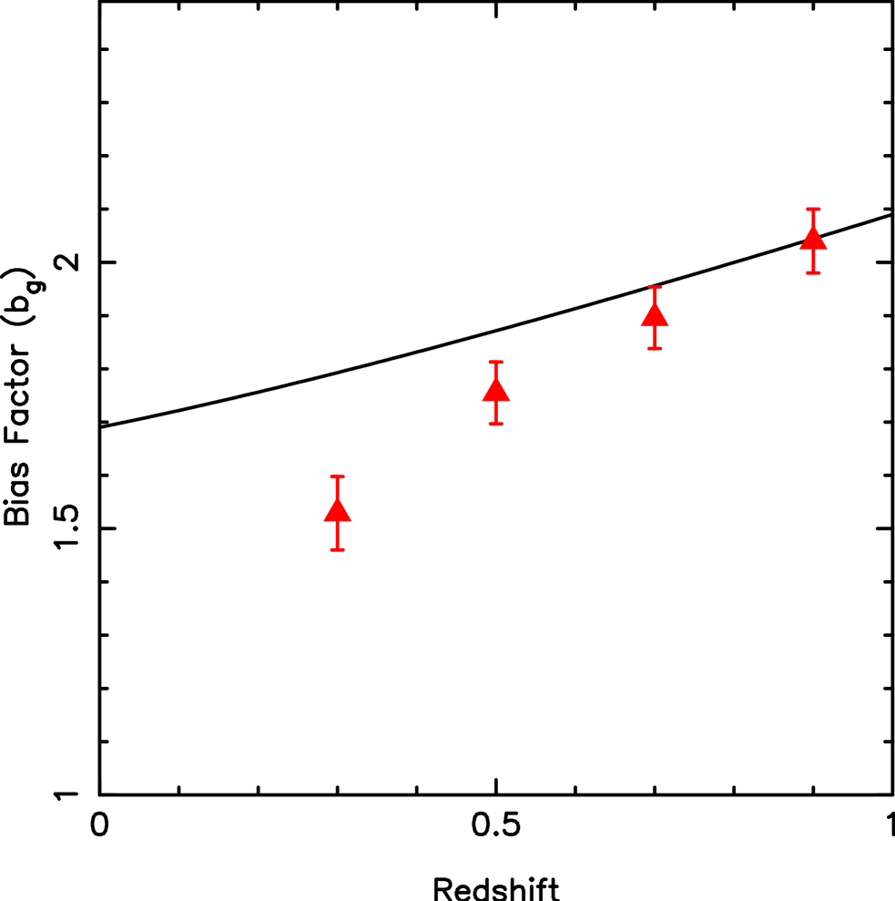
In White et al. (2007), we discussed the HOD of space density selected samples of red galaxies, and we recap several key results of that study here. We selected the most luminous red galaxies per unit volume down to a space density threshold of . If red galaxies underwent pure luminosity evolution (PLE) without galaxy mergers, a space density selected sample would select the same (fading) galaxy population with redshift and the spatial clustering would increase with decreasing redshift due to gravitational collapse. As we show in Figure 9, we find little or no evolution of the spatial clustering of these galaxies with redshift, which is contrary to PLE. The evolving bias factor of these galaxies does not evolve in the same manner as analytic approximations (Fry 1996) or simulations (White et al. 2007) of PLE. The PLE simulation, normalized to the observations, overestimates the number of satellite galaxies at by roughly . A simple solution is to remove a third of the satellites, by having them undergo merging or disruption between and (White et al. 2007).
In Figure 10 we plot the values of and as a function of -band absolute magnitude. As one would expect, the most massive central and satellite galaxies can only reside in the most massive halos, so and increase with luminosity. One can also see that the halo mass required to host a galaxy of fixed -band luminosity decreases with increasing redshift. It is not obvious from Figure 10 if this trend results from evolution of the relationship between galaxy stellar mass and halo mass, or the evolution of galaxy stellar populations.
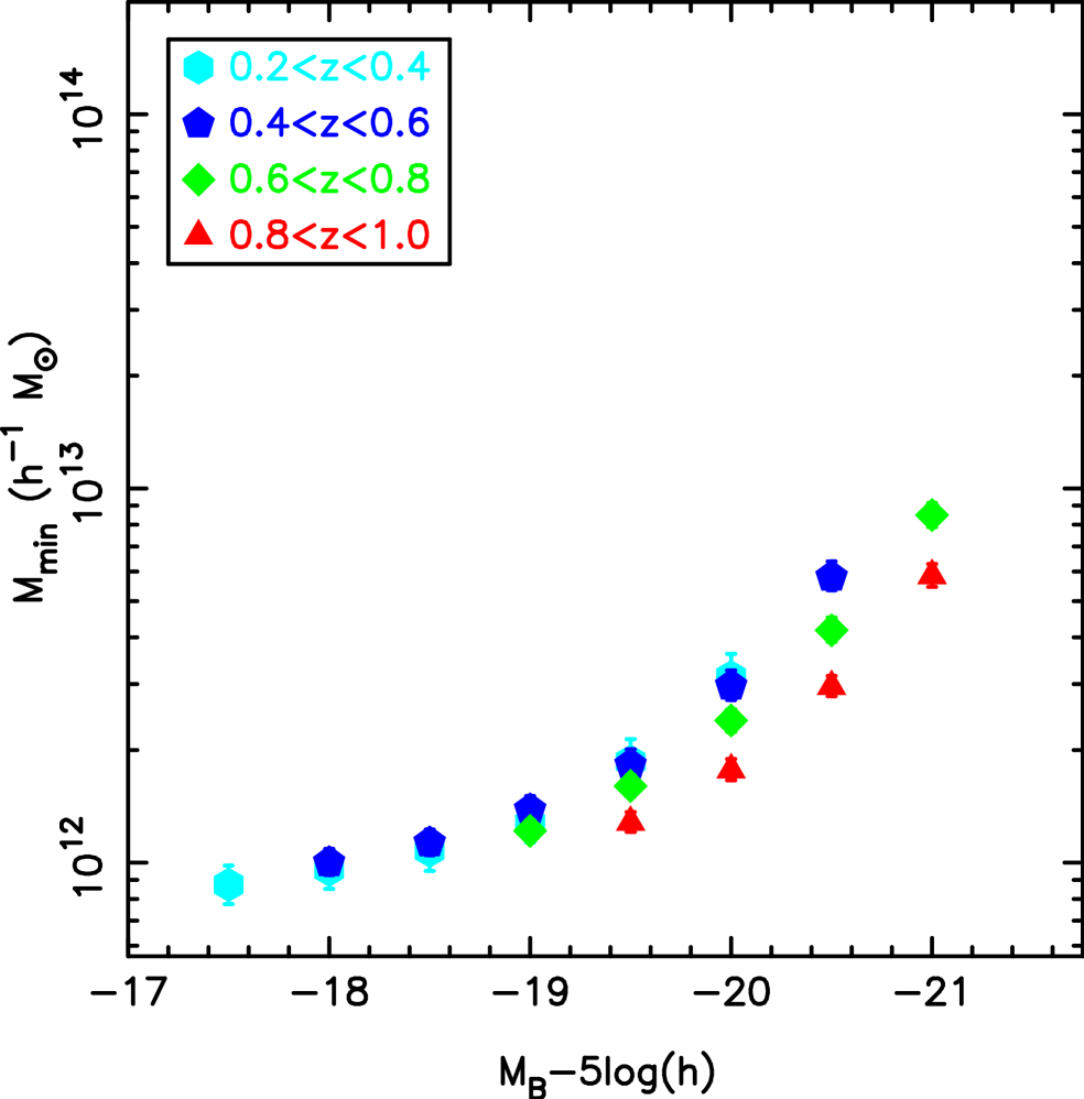
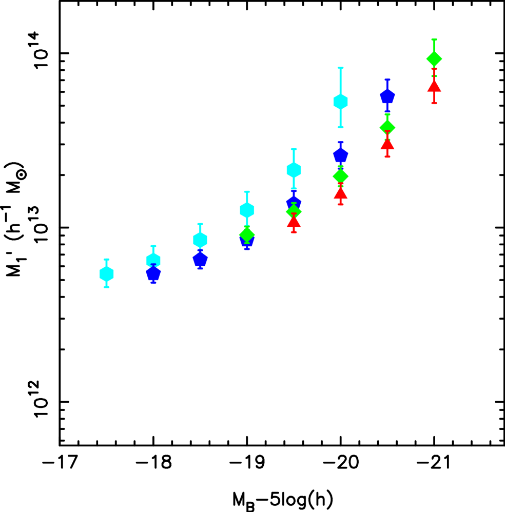
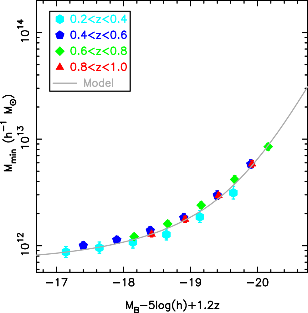
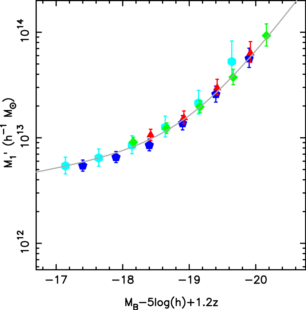
In Figure 11 we compensate for the fading of red galaxy stellar populations by adding to the -band absolute magnitudes. This correction is comparable to the observed evolution of the fundamental plane (e.g., van Dokkum & Stanford 2003; Treu et al. 2005) and is similar to the luminosity evolution of stellar populations models which reproduce the optical colors of red galaxies (e.g., Bell et al. 2004; Brown et al. 2007). The value of is effectively a proxy for stellar mass, although the exact conversion to stellar mass will depend on details of the stellar initial mass function and the star formation history. One can see in Figure 11 that and show little or no evolution as a function of red galaxy stellar mass. We thus conclude that the relationship between red galaxy stellar mass and host halo mass undergoes little or no evolution between and .
5.4 COMPARISON WITH HODs FROM THE LITERATURE
An important consistency check is to compare our HODs with those from the literature. Unfortunately, such a comparison is not straightforward due to differences in sample selection, adopted cosmology, and the assumed functional form of the HOD. To simplify the comparison, we plot HODs as a function of galaxy space density rather than attempting to model the equivalent absolute magnitude threshold in the -band. As space density is strongly correlated with luminosity, this provides a simple and well defined way of comparing samples selected using a variety of techniques.
HODs in the literature often use cosmologies or halo definitions that differ from the ones adopted here. To shift halo masses to our and cosmology, we use the prescription of Zheng et al. (2002). For this comparison, we define halos to be spherical objects with a mean density 200 times that of the background, and we modify halo masses from the literature to be consistent with this definition. We compare characteristic quantities which are not sensitive to the details of the HOD parameterization. We use and , where is the halo mass where and is the halo mass where .
In Figures 12 and 13 we compare our HOD estimates of and with those from the literature. The HODs from the literature are mostly derived from red galaxy samples, although we have included some HODs determined using samples including both red and blue galaxies (e.g., DEEP2, SDSS main). The various studies are in broad agreement, including measurements derived from the two-point correlation function (Zehavi et al. 2005a; Phleps et al. 2006; van den Bosch et al. 2007; Zheng et al. 2007; Blake, Collister, & Lahav 2008; Wake et al. 2008; Padmanabhan et al. 2008, Z. Zheng et al., in prep.), three-point correlation function (Kulkarni et al. 2007), satellite galaxy velocities (Conroy et al. 2007b) and lensing (Mandelbaum et al. 2006a). The agreement between our measurements and those derived from lensing and satellite galaxy velocities is encouraging, as those measurements of halo masses do not depend on models of the halo mass function.
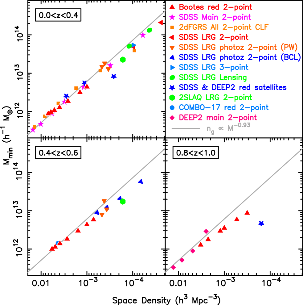
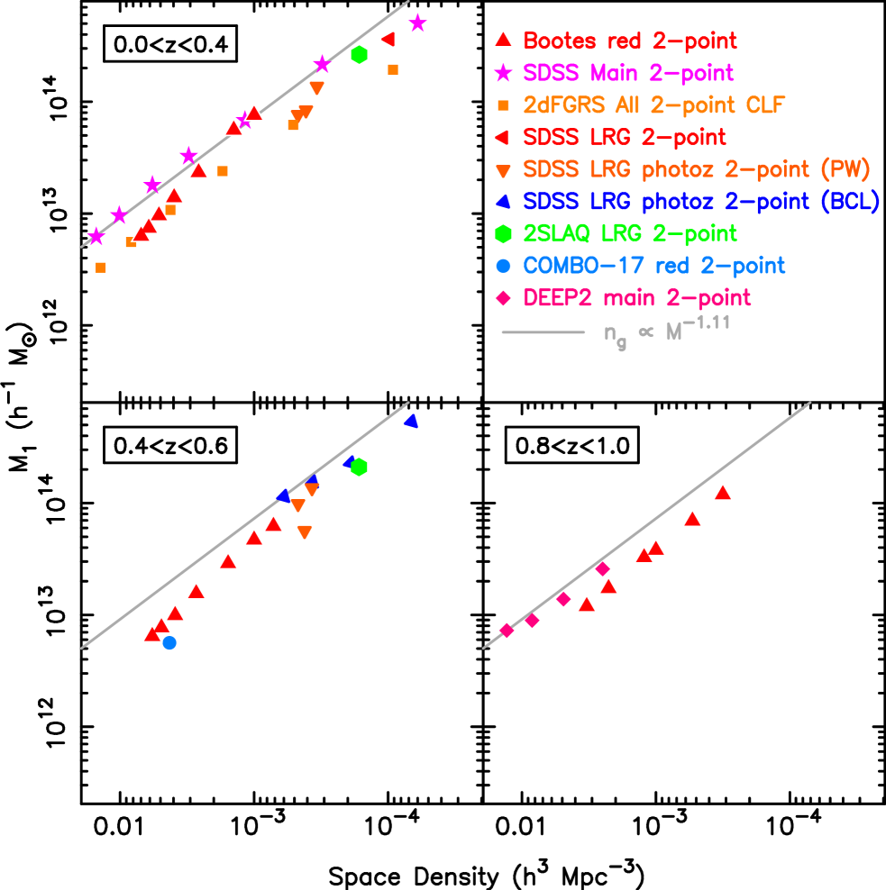
The relationship between galaxy space density and at can be approximated by a power-law
| (11) |
and this relationship appears to evolve slowly with redshift. Again, this is to be expected, as the mass function of dark matter halos less massive than evolves slowly and can be approximated by . This relationship should not hold for the most massive galaxies at high redshift, since the top end of the halo mass function is not a power-law and rapidly evolves.
While the results from the literature are in broad agreement, there is no consensus on how the relationship between galaxy stellar mass and host halo mass evolves. Some studies find this relationship evolves (Yan, Madgwick, & White 2003; Conroy et al. 2007b; Zheng et al. 2007)222Yan et al. (2003) find that the relationship between and host halo mass doesn’t evolve, but does not correspond to a fixed stellar mass. Conroy et al. (2007b) find that the relationship between stellar and host halo mass does not evolve for all but the most massive galaxies., while others find little or no evolution (Lin et al. 2006; Phleps et al. 2006). Measuring HOD evolution is complicated by several factors, which may explain the varying conclusions in the literature. Redshift dependent selection effects can produce errors in the observed rate of HOD evolution. Studies of the evolving HOD may also be comparing (somewhat) different galaxy populations at different epochs. Finally, the relationship between blue galaxy stellar mass and host halo mass may evolve at , while the same relation for red galaxies undergoes little or no evolution.
6 RED GALAXY EVOLUTION FROM HOD MODELING
As we show in Figure 11, there is little or no evolution of the relationship between red galaxy stellar mass and host halo mass at . Motivated by this, we introduce an analytic approximation of the HOD where the mean number of galaxies (of a given stellar mass) residing within halos (of a given mass) does not evolve. The simplicity of this model allows one to easily discern important relationships present in our data, including the correlation of central galaxy luminosity with host halo mass (§6.2) and the contributions of central and satellite galaxies to the total stellar mass within a halo (§6.3). Our analytic approximation also predicts how the luminosity function of central and satellite galaxies evolves over a broad redshift range (§6.4 and §6.5).
Our approximation does not include all the relevant astrophysics (e.g., dynamical friction) and has empirical components (e.g., the functional form of ), so it should not be confused with a complete model of galaxy evolution. We expect departures from this approximation (particularly at high ) and these will be informative. In this respect our approximation is somewhat analogous to the illustrative and simple pure luminosity evolution models. That said, our model does include many of the key components required to describe the evolution of red galaxies, including the aging of stellar populations and the growth of dark matter halos.
6.1 AN ANALYTIC APPROXIMATION OF THE HOD
Our analytic approximation of the HOD is largely constrained by the and measurements presented in Figure 11. These measurements span a limited luminosity range, so we use other measurements to constrain the HOD of the most massive galaxies. The satellite fraction decreases with luminosity, with at least 80% of red galaxies being central galaxies. We thus constrain the HOD of the most luminous galaxies by assuming one very luminous galaxy per halo, assuming some scatter () in the relation between central galaxy luminosity and halo mass, and matching the cumulative luminosity function of these galaxies with the cumulative mass function of dark matter halos.
We approximate the HOD parameters and (for galaxies brighter than an absolute magnitude threshold ) with a series of power-laws,
and
| . | (13) |
Each power-law component provides the relationship between galaxy luminosity and halo mass for a particular luminosity range. For example, the last term of Equation LABEL:eq:mmin shows halo mass is proportional to central galaxy luminosity to the power of for the most luminous galaxies. As we show in Figure 11, this approximation reproduces the measured values of and with an accuracy (RMS) of 8% and 7% respectively. As the other HOD parameters are poorly constrained by our observations, we fix their values to , and .
We caution that Equations LABEL:eq:mmin and 13 are only approximations of the true HOD. They also depend upon the assumed cosmology and the analytic approximations discussed earlier. It is also plausible that the HOD of red galaxies evolves very slowly at . That said, we do expect the broad brush-strokes of our model to be valid and it is these which we discuss below.
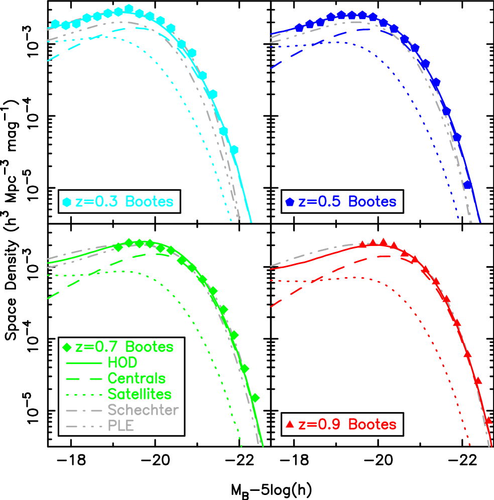
Using the mean number of galaxies (brighter than a luminosity threshold) per halo and the halo mass function, one can determine the cumulative luminosity function by estimating the space density of galaxies for a series of absolute magnitudes. Taking the derivative of this as a function of absolute magnitude, one obtains the conventional luminosity function. In Figure 14 we compare the observed red galaxy luminosity function with our HOD model and Schechter function fits. The accuracy of the HOD model is comparable to that of Schechter functions which were individually fitted to the data in each redshift bin. The HOD model has a consistently higher space density of very luminous galaxies than the Schechter function fits, particularly at . While the faint-end of Schechter luminosity functions is a power-law with a constant index, the power-law index of the HOD model luminosity function varies at faint magnitudes.
In Figure 15 we plot the red galaxy luminosity function and the HOD model split by host halo mass. As one would expect, only the most massive halos can host the most massive galaxies. However, while some of the faintest red galaxies are central galaxies in lower mass halos (), a large fraction of low luminosity red galaxies reside (as satellites) in relatively massive halos. Galaxies in cluster mass halos () represent a small fraction of the overall red galaxy population.
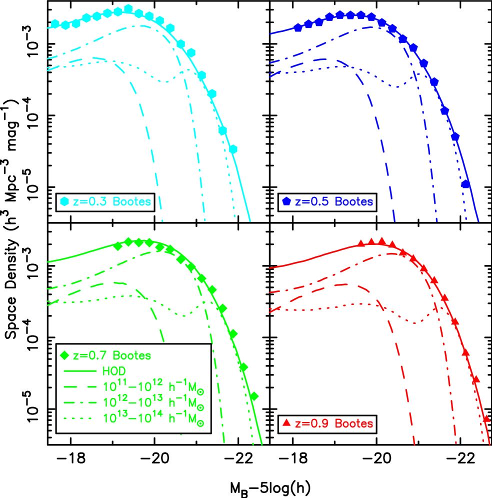
As we show in Figure 15, the shape of the red galaxy luminosity function varies with halo mass. In low mass halos, the shape of the galaxy luminosity function can be approximated by a Schechter function with a while in high mass halos . The value of in high mass halos is very similar to the measured luminosity function of red cluster galaxies (e.g., De Propris et al. 2003).
The luminosity function of group and cluster galaxies ( mass halos) has a wiggle at , corresponding to the transition from a satellite dominated luminosity function to a central dominated luminosity function. Although predicted by theory (Zheng et al. 2005) and observed in groups (Yang et al. 2007), the size and location of the wiggle depends on both and , which are poorly constrained by our data. The luminosity function of red field galaxies is often approximated by a Schechter function with , and in our HOD model this results from faint red galaxies residing in halos spanning a broad mass range.
6.2 THE GROWTH OF CENTRAL GALAXIES
In Figure 14 we plot the central and satellite components of the red galaxy luminosity function, determined using our analytic approximation of the HOD. Clearly the top end of the luminosity function is dominated by central galaxies. As we noted previously, halo mass scales as central galaxy luminosity to the power of , so the stellar masses of central galaxies scale as halo mass to the power of . We constrain the luminosity-mass relation for the brightest red galaxies using the observed luminosity function (§3) and the predicted halo mass function, so our luminosity-mass relation for these galaxies is similar to the empirical model of Vale & Ostriker (2004, 2006) by construction. Our luminosity-mass relation for the most massive red galaxies is broadly similar to others in the literature, where halo mass was determined using X-ray temperature (Lin & Mohr 2004; Lin et al. 2006), X-ray luminosity (Brough et al. 2008), and weak lensing (Mandelbaum et al. 2006b).
As the relationship between central galaxy stellar mass and halo mass is approximated by a non-evolving power-law with an index of , the most massive galaxies do not grow as rapidly as their host halos. While a merger of comparable mass halos presumably results in a merger of central galaxies, it is plausible that such mergers are not 100% efficient and dump stellar mass into the diffuse ICL (e.g., Gonzalez et al. 2000; Arnaboldi et al. 2002; Feldmeier et al. 2004; Zibetti et al. 2005; Monaco et al. 2006; White et al. 2007; Conroy, Wechsler, & Kravtsov 2007c; Conroy, Ho, & White 2007a). Minor halo mergers may produce satellite galaxies instead of directly funneling stellar mass into the central galaxy. As a result, while mergers may increase the mass of a halo by 100% at , the stellar mass of the central galaxy typically grows by only 30%. This is consistent with recent measurements of the luminosity function, where the most massive galaxies do not grow as rapidly as the most massive dark matter halos (e.g., Brown et al. 2007). Semi-analytic models and simulations with rapid growth of massive galaxies may be overestimating the ability of halo mergers to funnel stellar mass into central galaxies (e.g., Taylor & Babul 2001; Benson et al. 2003; Taffoni et al. 2003; Boylan-Kolchin et al. 2008).
Our approximation of the HOD and the observed luminosity function of red galaxies (Figure 14) are inconsistent with pure passive evolution without mergers. However, it remains plausible that the efficiency of central galaxy growth via halo mergers continues to decline with increasing halo mass (e.g., Cooray & Milosavljević 2005). As the rate of major mergers with halos declines with decreasing redshift, the rate of massive galaxy growth will taper off. It is thus plausible that the space density of the most massive galaxies at low redshift can be approximated by pure passive evolution above some mass threshold (e.g., Bundy et al. 2006; Cimatti et al. 2006; Wake et al. 2006).
Our analytic approximation of the HOD has a lower mass limit, so the cumulative luminosity function of central red galaxies only marginally increases with decreasing luminosity at . Halos far less massive than presumably host blue central galaxies. The color bimodality of galaxies also shows evidence for a transition mass (e.g., Kauffmann et al. 2003), which is broadly consistent with our results. If star formation were truncated as function of galaxy stellar mass, one would not expect to observe red dwarf spheroidals. Thus, the bimodality of galaxy colors may be better described by a truncation of central galaxy star-formation in halos above a critical mass. Presumably there is a mechanism which prevents gas from cooling in high mass halos, thus suppressing central galaxy star-formation. The most plausible mechanisms in the current literature are virial shock heating (e.g., Birnboim & Dekel 2003; Khochfar & Ostriker 2007; Dekel & Birnboim 2006) and feedback from AGNs (e.g., Silk & Rees 1998; Wyithe & Loeb 2003; Croton et al. 2006; Hopkins et al. 2006).
6.3 STELLAR MASS IN CENTRAL AND SATELLITE GALAXIES
In Figure 16 we plot the -band luminosity contributed by red galaxies as a function of halo mass at , determined using our analytic approximation of the HOD. We also plot measurements of -band luminosity versus mass, where the halo mass was determined with weak lensing (Mandelbaum et al. 2006b), satellite galaxies (Conroy et al. 2007b) and X-ray temperature (Lin, Mohr, & Stanford 2004; Lin & Mohr 2004). To include these measurements on our plot we assume and . There is broad agreement between these measurements and our analytic approximation of the HOD, which we constrained with measurements of the space density and clustering of red galaxies.
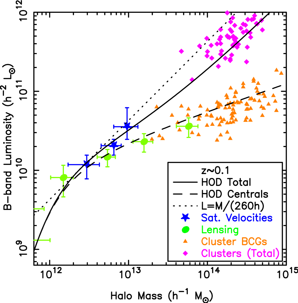
As we show in Figure 16, the fraction of -band light contributed by satellite galaxies rapidly increases with halo mass. This is not unexpected, as the bulk of stellar mass within clusters does not reside within the brightest cluster galaxy (e.g., Sandage et al. 1985; Lin et al. 2004; Lin & Mohr 2004). Clearly the growth of these halos did not result in stellar mass being efficiently funneled into the central galaxy.
In high mass halos the total -band luminosity is proportional to halo mass to the power of rather than . This may indicate that mergers with very massive halos shift stellar mass out of the red galaxy population, perhaps into the ICL (e.g., Gonzalez et al. 2000; Arnaboldi et al. 2002; Feldmeier et al. 2004; Zibetti et al. 2005; Monaco et al. 2006; White et al. 2007; Conroy et al. 2007a, 2007c).
6.4 THE EVOLVING LUMINOSITY DENSITY OF RED GALAXIES
The luminosity weighted integral of the luminosity function, the luminosity density, is often used to estimate the evolution of the stellar mass within the red galaxy population. In Figure 17 we plot -band luminosity density measurements from Boötes and the literature (Madgwick et al. 2002; Bell et al. 2004; Blanton 2006; Willmer et al. 2006; Faber et al. 2007). Roughly 15% of the luminosity density is contributed by galaxies fainter than our magnitude limits, and we have applied corrections to the Boötes measurements using our HOD approximation of the luminosity function. While there are some discrepancies between the various surveys, which we discuss below, there is a broad consensus that the -band luminosity density of red galaxies evolves slowly at (Bell et al. 2004; Brown et al. 2007; Faber et al. 2007).
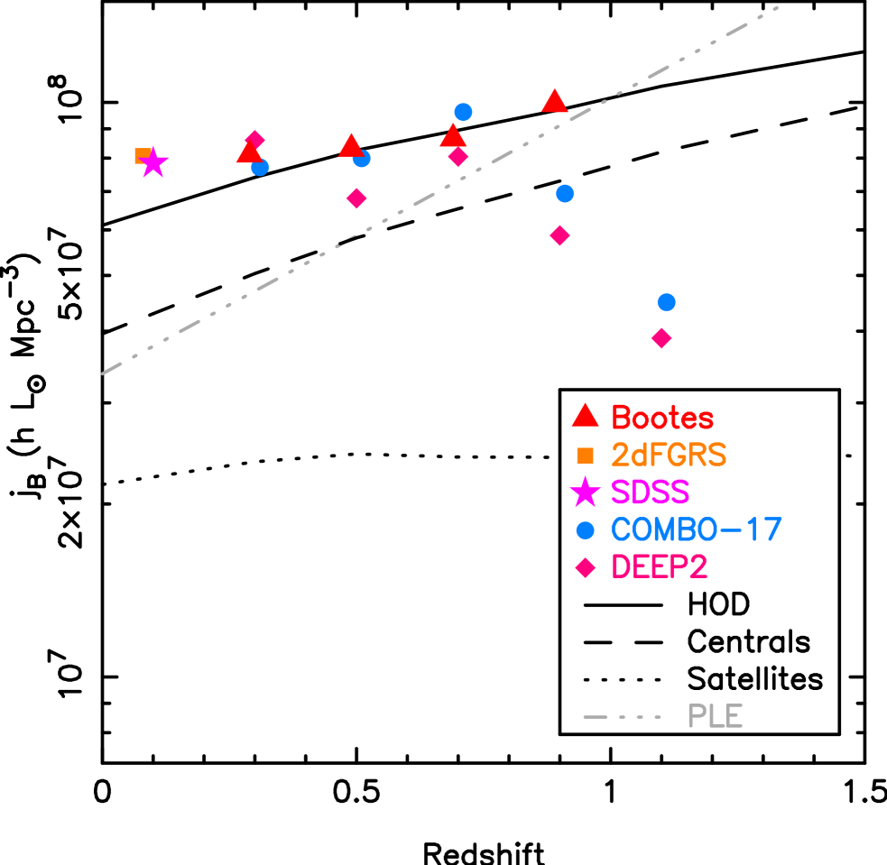
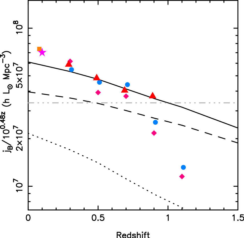
In Figure 17 we over-plot the evolving luminosity density derived from our analytic approximation of the HOD. As the stellar populations of red galaxies fade between and , a non-evolving luminosity density does not correspond to a fixed stellar mass density. To simplify the interpretation of the luminosity density, in the right-hand panel of Figure 17 we divide the -band luminosity density by , so the y-axis is proportional to stellar mass. One can clearly see that the stellar mass contained within the red population doubles between and . As red galaxies have low rates of star-formation, presumably this mass is being transferred from the blue galaxies after a decline in star-formation (e.g., Bell et al. 2004; Brown et al. 2007; Faber et al. 2007).
In Figure 17 we show the contributions of central and satellite galaxies to the evolving luminosity density. If the stellar mass contained within the satellite and central populations remained fixed at their values, the luminosity density of both populations would be lower than what we derive from HOD modeling. The stellar mass contained within the red satellite population triples between and . The bulk of red satellites were either central or blue galaxies within the past .
A naive interpretation of our results is that equal portions of new stellar mass are being transfered from the blue population to the red central and satellite populations. Such an interpretation is risky, since satellites can merge with central galaxies, and central galaxies can become satellites in groups or clusters. One can imagine extreme scenarios where star-formation is only truncated in central or satellite galaxies. More sophisticated models, which track the evolution of individual halos and galaxies over cosmic time will address these issues, and we will discuss such a model in an upcoming paper (M. White et al. in prep.).
6.5 COMPARISON WITH OTHER SURVEYS
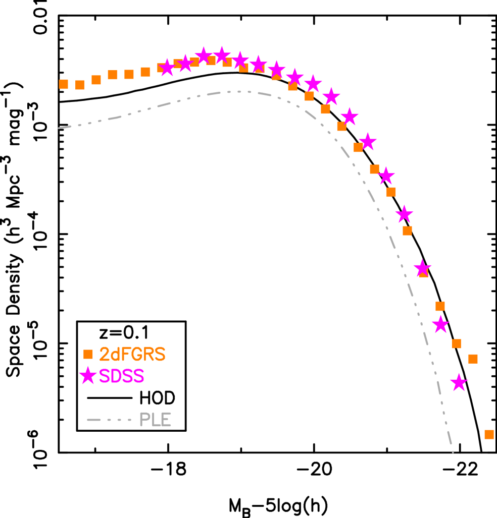
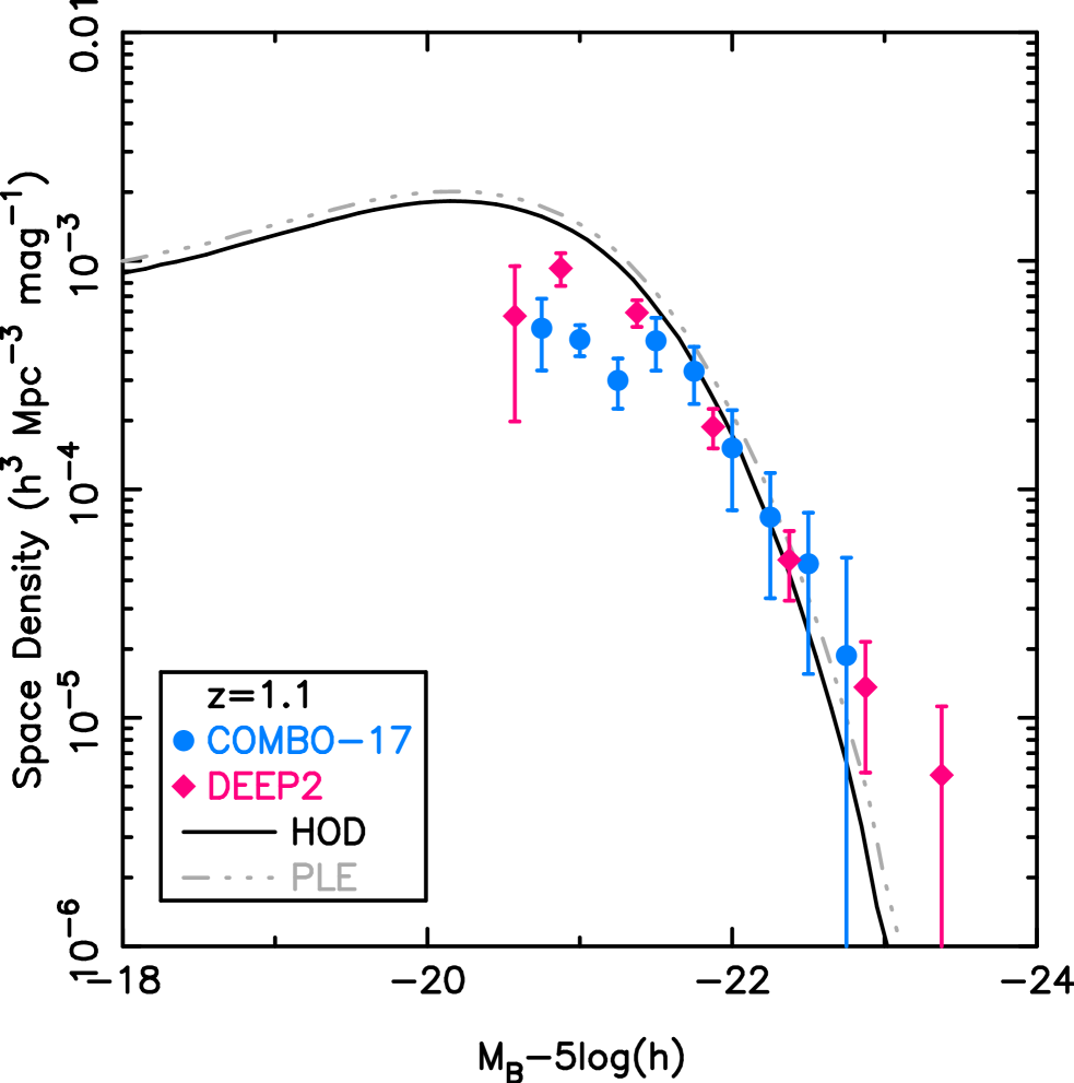
In Figure 18 we plot measurements of the red galaxy luminosity function at low and high redshift (Madgwick et al. 2002; Blanton 2006; Bell et al. 2004; Willmer et al. 2006; Faber et al. 2007) along with the predictions of our HOD approximation and PLE. The PLE model, normalized to our measurements, does not reproduce the red galaxy luminosity function. The PLE model underestimates the space density of red galaxies and underestimates the luminosities of the most massive galaxies at low redshift.
Our HOD model better approximates the galaxy luminosity function than a PLE model. However, while our model reproduces the bright end of the luminosity function, there are systematic offsets at low luminosities. As the most luminous red galaxies lie along the red sequence, their measured space density is insensitive to details of the galaxy selection criteria. In contrast, there is a significant population of galaxies with colors falling between the red and blue galaxy populations. By shifting our rest-frame selection criterion blueward by just 0.1 magnitudes, the measured space density of red galaxies increases by 25% while the measured values decrease by 10%. Such a shift would remove the offset between our HOD approximation and the 2dFGRS and SDSS measurements.
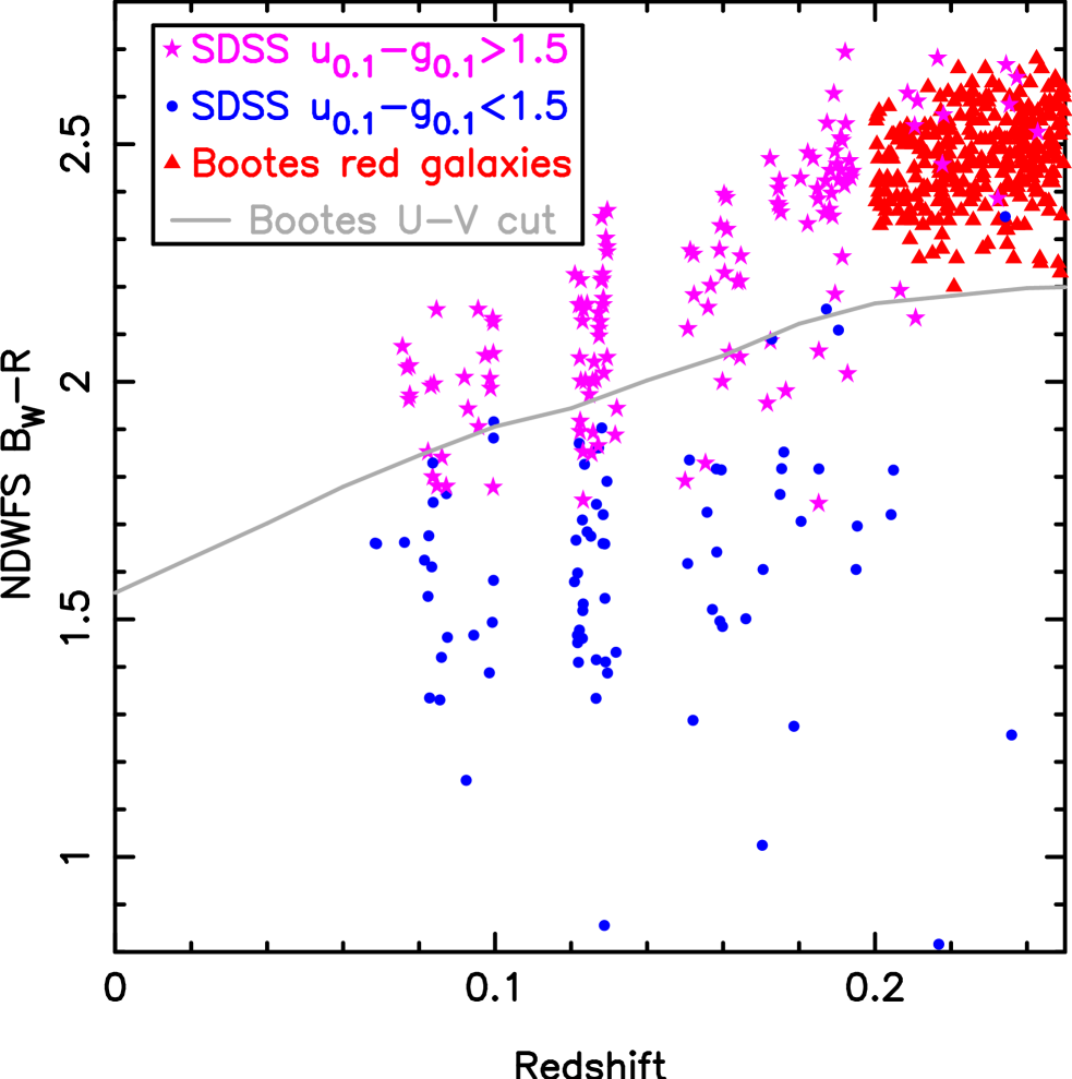
As the SDSS includes the Boötes field, we can directly compare our red galaxy sample with that of Blanton (2006). As we show in Figure 19, the Blanton (2006) red galaxy sample includes systematically bluer galaxies than our sample. This explains why Blanton (2006) measures a higher space density of red galaxies than Boötes. The rest-frame criterion of Blanton (2006) may be bluer than our criterion, although other factors could be significant including the choice of galaxy SED templates and the method used to measure galaxy photometry.
It is unclear if the HOD undergoes rapid evolution at . We find a significantly higher space density of red galaxies than either COMBO-17 or DEEP2. If the DEEP2 or COMBO-17 measurements of the luminosity function are valid, the HOD must rapidly evolve at . As we noted previously, we do expect some evolution of the HOD as there is residual star-formation within the red galaxy population and the properties of dark matter halos of a given mass evolve. Why this evolution should rapidly accelerate at is unclear.
It is plausible that COMBO-17 and DEEP2 are underestimating the space density of red galaxies. DEEP2 uses a non-evolving selection criterion for red galaxies, and this criterion must be redder than the evolving colors of an aging stellar population at high redshift. We thus expect DEEP2 to underestimate the space density of red galaxies beyond some (as yet undetermined) redshift. There is an ongoing collaboration between the Boötes and DEEP2 surveys to resolve this discrepancy, and we have obtained imaging of the DEEP2 Extended Groth Strip with the NDWFS filter-set to determine the impact of photometric errors on current luminosity function measurements. Unfortunately, COMBO-17 optical photometric redshifts have gross errors for galaxies beyond (E. F. Bell, N. Taylor - private communication), resulting in a spuriously rapid decline in the space density of red galaxies. This systematic error is being addressed with the addition of near-infrared photometry to the COMBO-17 photometric redshifts. At present, it remains plausible that the relationship between galaxy stellar mass and host halo mass evolves slowly out to , and there is a clear need for robust space density and clustering measurements to test this conjecture.
7 SUMMARY
We have measured the past of red galaxy growth within dark matter halos. To do this, we have measured the halo occupation distribution, which describes how galaxies reside within dark matter halos (as a function of halo mass). We have constrained HOD models using measurements of the evolving luminosity function and clustering of red galaxies. Our sample of 40,696 red galaxies, selected from of imaging in Boötes, is far larger than comparable galaxy samples at these redshifts.
We have measured the evolving luminosity function of red galaxies, and obtain results that are very similar to Brown et al. (2007). The bright end of the luminosity function fades with time, indicating that the most massive galaxies are not rapidly growing via mergers. The bright end of the luminosity function does not fade as rapidly as an aging stellar population, and we conclude that the stellar masses of the most massive galaxies have grown by 30% over the past . We find that the luminosity density of red galaxies evolves slowly with redshift, and the stellar mass contained within the red galaxy population has doubled between and . As there is little star-formation within the red galaxy population, stellar mass must have been transfered from the blue galaxy population at .
We have measured the angular correlation function of red galaxies, using samples selected as a function of photometric redshift, luminosity and space density. We evaluated power-law and HOD models of the spatial correlation function by using the Limber (1954) equation to determine corresponding angular correlation functions. To evaluate the quality of the models, we determined values using the complete covariance matrices for the angular correlation function. Preliminary covariance matrices were determined using analytic approximations while our final results were determined using covariance matrices derived from mock catalogs. Our mock catalogs reproduce the luminosity and correlation functions of red galaxies, and include large-scale structures that are frequently observed in deep galaxy surveys.
We find that the value of increases with luminosity for red galaxies brighter than , while for fainter galaxies . While the spatial clustering of red galaxies as a function of luminosity clearly evolves, this is largely due to the fading of aging stellar populations rather than the evolution of large-scale structures.
We performed HOD modeling of the observed luminosity function and angular clustering of Boötes red galaxies. The large-scale bias factor increases with luminosity for red galaxies brighter than . We find that the bias of red galaxies increases with redshift, as the spatial clustering of galaxies does not evolve as rapidly as the underlying distribution of dark matter. The evolution of the bias factor is inconsistent with pure luminosity evolution models without mergers (White et al. 2007), where the spatial clustering increases with time due to gravitational collapse.
The relationship between red galaxy luminosity and host halo mass evolves, due to the fading of aging stellar populations. We do not observe any evolution of the relationship between red galaxy stellar mass and host halo mass with redshift. As halo masses grow at , we expect the stellar masses of central galaxies to also grow at .
We find that the HOD of red central galaxies has a lower limit, with 50% of mass halos hosting a red central galaxy. As one moves down further in halo mass, one presumably observes an increasing fraction of blue central galaxies. What truncates star-formation in central galaxies is unclear, but it appears to be strongly correlated with host halo mass.
We can reproduce both the luminosity function and clustering of red galaxies in Boötes with an analytic approximation of the HOD, which also simplifies the interpretation our of HOD measurements. In our model, the fraction of stellar mass within the satellite population increases with host halo mass. In cluster () mass halos, more mass resides within satellites than central galaxies. We thus conclude that mergers with these halos do not always (efficiently) funnel stellar mass into central galaxies. The luminosities of central galaxies are proportional to halo mass to the power of . As a result, if halo masses increase by 100% at , the stellar mass of the typical central galaxy grows by only 30% over the same redshift range. Massive galaxy assembly continues at , but the bulk of their growth took place at higher redshifts.
The growth of stellar mass within the red population at is reproduced by our analytic approximation of the HOD. The stellar mass contained within red satellite galaxies triples between and , and they account for a third of the stellar mass within the red population by . Our analytic approximation of the HOD reproduces current measurements of the bright-end of the red galaxy luminosity function, but there are offsets at lower luminosities. Either measurements of the red galaxy luminosity function have large systematic errors, or the red galaxy HOD rapidly evolves at .
Appendix A AN ANALYTIC APPROXIMATION FOR THE COVARIANCE MATRIX
Our final estimates of the angular correlation function covariance matrices are derived from mock catalogs. However, one needs estimates of the HOD to generate such mocks, so preliminary fits of HOD models to the angular correlation function utilized analytic approximations of the covariance matrices. The basis of our analytic covariance matrices is the Gaussian approximation (e.g., Eisenstein & Zaldarriaga 2001):
| (A1) |
where is a Bessel function and is the (2D) angular power spectrum,
| (A2) |
This approximation is best suited to correlation functions where and underestimates the covariance of very strongly clustered objects. For a power-law power spectrum, or , the integral can be evaluated analytically in terms of and :
| (A3) |
valid for . The power-series expansion of the (confluent) hypergeometric function, , converges rapidly. For cases where the power-law is (nearly) divergent we truncate the integral at an angular scale corresponding to a transverse comoving distance of Mpc. In practice, fits to our data are only marginally affected by the value of the angular correlation function on scales of more than . If the angular correlation function bins have significant width, Equation A1 is modified to
| (A4) |
(D. Eisenstein 2003, private communication) where and are the inner and outer radii of the bins. This can be rewritten as the single integral
| (A5) |
The contribution of shot noise to the estimate of the covariance was included by adding the reciprocal of the sky surface density of galaxies (per steradian) to . However, the shot noise only dominates the covariance on scales of for the red galaxy sample.
The analytic covariance matrix of Eisenstein & Zaldarriaga (2001) underestimates the uncertainties when . To mitigate this issue, we approximate the covariance matrix with,
| (A6) |
where is determined using the method of Eisenstein & Zaldarriaga (2001) and is determined using the truncated power-law discussed earlier. The second term of this equation was determined by trial and error, and roughly approximates the near-diagonal elements of the Boötes covariance matrices derived from jack-knife subsamples and mock catalogs. While this term is a hack and should be treated with caution (and perhaps contempt), it does prevent highly correlated measurements on small angular scales from skewing preliminary fits of power-laws and HODs to our data.
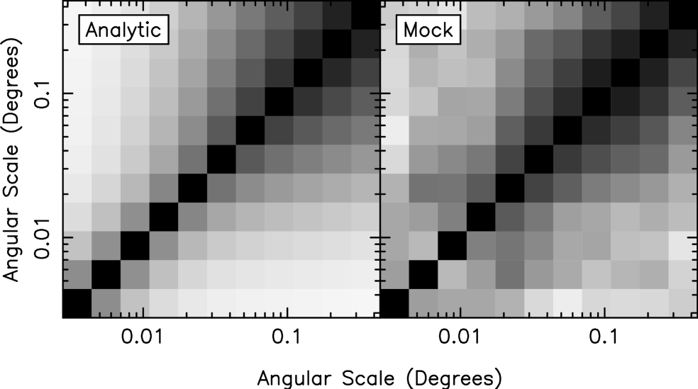
In Figure 20 we plot the analytic and mock correlation matrices for one of our red galaxy samples. While the diagonal elements of the covariance matrices are comparable, the off-diagonal elements of the analytic covariance matrix are systematically less than those determined with mock galaxy catalogs. The uncertainties of power-law fits to the binned angular correlation function increase by up to 100% when we switch from analytic to mock covariance matrices. However, HOD parameters exhibit little change when we switch covariance matrices, as the HOD is constrained by the dark matter distribution, halo mass function and observed galaxy space density as well as the observed clustering of galaxies.
Appendix B MOCK CATALOGS
We used mock galaxy catalogs to estimate the covariance matrix of the correlation function and the uncertainties for luminosity functions. We utilized a simulation which is very similar to that of White et al. (2007), but with a larger volume and lower mass resolution. The same cosmology is used as throughout this paper: , , , and . As in White et al. (2007), the linear theory power spectrum for the initial conditions was computed by evolution of the coupled Einstein, fluid and Boltzmann equations using the code described in White & Scott (1996). Seljak et al. (2003) find that this code agrees well with CMBfast (Seljak & Zaldarriaga 1996). The simulation employed particles of mass in a periodic cube of side Gpc using a TreePM code (White 2002) with a Plummer-equivalent softening length of kpc (comoving). A detailed comparison of this TreePM code with other codes can be found in Heitmann et al. (2007).
We used a series of simulation outputs at and for each output we generate a halo catalogs using the Friends-of-Friends (FoF) algorithm (Davis et al. 1985) with a linking length of 0.168 times the mean inter-particle spacing. This procedure partitions the particles into equivalence classes, by linking together all particle pairs separated by less than a distance . The halos correspond roughly to particles with times the background density. Our mass definition uses the sum of the particle masses in the halo, however to obtain better correspondence between our definition of halo mass and that implicitly defined by the mass functions of Sheth & Tormen (1999) and Jenkins et al. (2001) we rescaled the masses by where is the FoF mass in units of . With this redefinition the mass function in the simulation lies between those of Sheth & Tormen (1999) and Jenkins et al. (2001), differing from them by less than 10% in the mass range of interest.
Mock catalogs were constructed by using an analytic approximation of the HOD (§6) to assign central and satellite galaxies to halos. We determined the mean number of central red galaxies as a function of halo mass and used a random number generator to determine if a central galaxy was assigned to a particular halo. We determined the mean number of satellite galaxies as a function of halo mass, and used a random number generator and Poisson statistics to determine the number of satellites assigned to each halo. To determine the likelihood of a galaxy having a particular luminosity, we used conditional luminosity functions (number of galaxies per magnitude per halo) for central and satellite galaxies. These luminosity functions are a function of host halo mass and were derived from the cumulative luminosity functions provided by the analytic approximation of the HOD. Central galaxies were placed precisely at the center of dark matter halos while the distribution of satellite galaxies follows a spherical NFW profile. Random number generators were used to assign galaxy luminosities and satellite positions relative to halo centers.
The simulation was used to produce between 56 () and 400() Boötes sized samples. The simulation cube was viewed parallel to one of the Cartesian axes, and each galaxy was assigned a spectroscopic redshift and corresponding apparent magnitude. Galaxies were then assigned photometric redshifts, assuming Gaussian random errors and the photometric redshift uncertainties reported by Brown et al. (2007), and the absolute magnitudes were scattered accordingly. In Figure 21 we show the sky distribution of three red galaxy mocks and the real red galaxy catalog. Individual large-scale structures at are seen in both the Boötes field and our mock catalogs, and are relatively common in other deep surveys (e.g., Lubin et al. 2000; Nakata et al. 2005; Guzzo et al. 2007). While large structures of high redshift galaxies were once expected to be rare, this assumed rapid galaxy growth took place at .
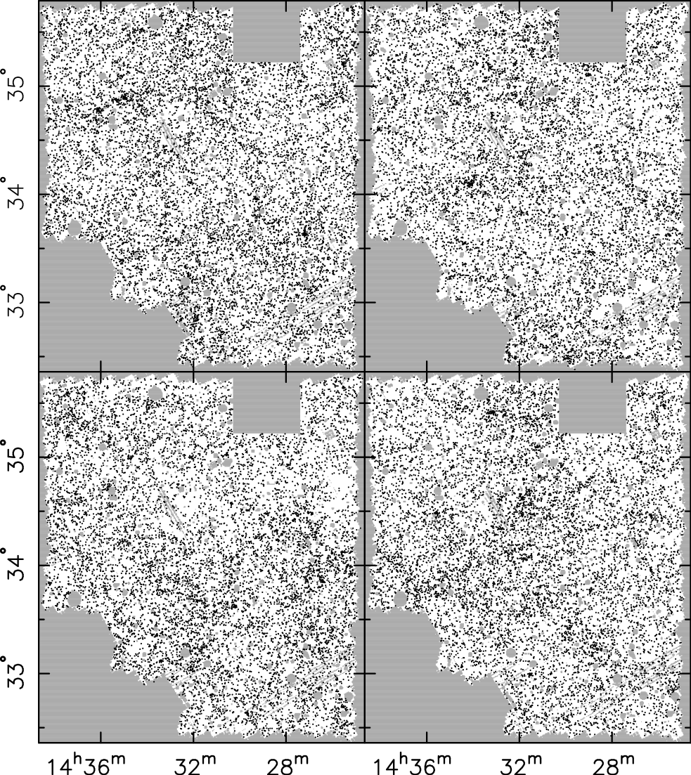
Angular correlation functions were determined for each Boötes sized mock using the Landy & Szalay (1993) estimator, and these were used to derive covariance matrices. These covariance matrices include both sample variance and shot-noise without needing to assume the underlying fluctuations are Gaussian or higher-order moments follow some particular pattern. We also use the mocks to estimate the uncertainties for the galaxy luminosity functions.
Are the mock catalogs consistent with the observed clustering of red galaxies in Boötes? To verify this we used the analytic approximation of the HOD to determine values for the angular correlation functions measured from each mock. We then determined in the same manner using the real Boötes field. In Figure 22 we plot the distribution of values for the mocks and Boötes. With the possible exception of the faintest red galaxies in our highest redshift bin, the Boötes values are comparable to those derived from the mocks. The analytic approximation of the HOD slightly underestimates the space density and overestimates the clustering of the faintest red galaxies. This discrepancy may be caused by selection effects, as a small shift in the rest-frame selection criteria can alter the measured space density and clustering of red galaxies by . As we discuss in §6.4, such selection effects may contribute to the large scatter of luminosity density measurements reported in the current literature.

| Absolute | Luminosity Function () | |||
|---|---|---|---|---|
| Magnitude | ||||
| - | - | - | ||
| - | - | - | ||
| - | - | |||
| - | - | |||
| - | - | |||
| - | - | |||
| - | ||||
| - | ||||
| - | ||||
| - | ||||
| - | ||||
| - | ||||
| range | Volume | |||||
|---|---|---|---|---|---|---|
| 6027 | ||||||
| 11117 | ||||||
| 11154 | ||||||
| 12398 |
| Subsample Selection | Photometric | Comoving | ||||
|---|---|---|---|---|---|---|
| Criterion | Redshift | |||||
| Narrow luminosity range | ||||||
| 1608 | 0.76 | |||||
| 1890 | 1.06 | |||||
| 2230 | 0.59 | |||||
| 2229 | 0.99 | |||||
| 1788 | 0.37 | |||||
| 1071 | 0.70 | |||||
| 3551 | 1.22 | |||||
| 4270 | 0.85 | |||||
| 4525 | 0.66 | |||||
| 3875 | 1.58 | |||||
| 2581 | 0.67 | |||||
| 1314 | 0.96 | |||||
| 5864 | 0.24 | |||||
| 5590 | 1.04 | |||||
| 4158 | 0.55 | |||||
| 2421 | 1.09 | |||||
| 1090 | 0.40 | |||||
| 7654 | 0.36 | |||||
| 6534 | 0.84 | |||||
| 4147 | 1.14 | |||||
| 1992 | 1.40 | |||||
| Wide luminosity range | ||||||
| 6027 | 0.86 | |||||
| 5275 | 0.87 | |||||
| 4419 | 0.84 | |||||
| 3385 | 0.82 | |||||
| 2189 | 0.68 | |||||
| 1157 | 0.87 | |||||
| 11117 | 1.29 | |||||
| 9541 | 1.11 | |||||
| 7566 | 1.11 | |||||
| 5271 | 1.02 | |||||
| 3041 | 0.81 | |||||
| 1396 | 1.10 | |||||
| 11154 | 0.73 | |||||
| 8321 | 0.80 | |||||
| 5290 | 0.45 | |||||
| 2731 | 0.74 | |||||
| 1132 | 0.57 | |||||
| 12398 | 0.81 | |||||
| 8619 | 0.79 | |||||
| 4744 | 1.26 | |||||
| 2085 | 1.27 | |||||
| Space density selected samples | ||||||
| 770 | 0.99 | |||||
| 1836 | 1.44 | |||||
| 2813 | 0.88 | |||||
| 3802 | 1.56 | |||||
| 955 | 0.75 | |||||
| 1233 | 0.71 | |||||
| Subsample Selection | Photometric | Space Density | aaAll masses are in units of . | ||||||
|---|---|---|---|---|---|---|---|---|---|
| Criterion | Redshift | ||||||||
| Subsample Selection | Photometric | Space Density | aaAll masses are in units of . | ||||||
|---|---|---|---|---|---|---|---|---|---|
| Criterion | Redshift | ||||||||
| 0.30 | 1.00 | ||||||||
| 0.30 | 1.00 | ||||||||
| 0.30 | 1.00 | ||||||||
| 0.30 | 1.00 | ||||||||
| 0.30 | 1.00 | ||||||||
| 0.30 | 1.00 | ||||||||
| 0.30 | 1.00 | ||||||||
| 0.30 | 1.00 | ||||||||
| 0.30 | 1.00 | ||||||||
| 0.30 | 1.00 | ||||||||
| 0.30 | 1.00 | ||||||||
| 0.30 | 1.00 | ||||||||
| 0.30 | 1.00 | ||||||||
| 0.30 | 1.00 | ||||||||
| 0.30 | 1.00 | ||||||||
| 0.30 | 1.00 | ||||||||
| 0.30 | 1.00 | ||||||||
| 0.30 | 1.00 | ||||||||
| 0.30 | 1.00 | ||||||||
| 0.30 | 1.00 | ||||||||
| 0.30 | 1.00 | ||||||||
| 0.30 | 1.00 | ||||||||
| 0.30 | 1.00 | ||||||||
| 0.30 | 1.00 | ||||||||
| 0.30 | 1.00 | ||||||||
| 0.30 | 1.00 | ||||||||
| 0.30 | 1.00 |