Dissipation and criticality in the lowest Landau level of graphene

Abstract

The lowest Landau level of graphene is studied numerically by considering a tight-binding Hamiltonian with disorder. The Hall conductance $\sigma_{\mathrm{xy}}$ and the longitudinal conductance $\sigma_{\mathrm{xx}}$ are computed. We demonstrate that bond disorder can produce a plateau-like feature centered at $\nu=0$, while the longitudinal conductance is nonzero in the same region, reflecting a band of extended states between $\pm E_{c}$, whose magnitude depends on the disorder strength. The critical exponent corresponding to the localization length at the edges of this band is found to be $2.47\pm 0.04$. When both bond disorder and a finite mass term exist the localization length exponent varies continuously between $\sim 1.0$ and $\sim 7/3$.

The quantum Hall effect (QHE), either integer or fractional, is one of the most intriguing phenomena in physics Laughlin (1999) that has drawn, and still continues to draw, enormous attention even after two decades since its discovery. In graphene unconventional QHE Novoselov et al. (2005); Zhang et al. (2005) corresponding to $\sigma_{\mathrm{xy}}=\pm(n+1/2)4(e^{2}/h)=\pm 4\nu(e^{2}/h),\;n=0,1,2,\ldots$, where $\sigma_{xy}$ is the Hall conductance, has been addressed in terms of low lying excitations akin to relativistic Dirac fermions Gusynin and Sharapov (2005); Peres et al. (2006); the factor of 4 arises from the two-fold valley and spin degeneracies; $e$ is the electronic charge and $h$ the Planck’s constant. Yet, a more complete theory of QHE requires an understanding of the localization-delocalization transitions within the Landau levels, which reflects a very special quantum phase transition, especially in graphene with its low energy Dirac spectra Ostrovsky et al. (2007); Goswami et al. (2007); Koshino and Ando (2007). It is indeed paradoxical that such a precise quantization requires material defects and disorder, and even the nature of disorder seems to matter for graphene.

A remarkable recent discovery in graphene is, what appears to be, a $\nu=0$ plateau in a sufficiently large magnetic field Zhang et al. (2006); Abanin et al. (2007), although the plateau in the measured $\rho_{xy}$ is difficult to decipher. The longitudinal resistivity $\rho_{\mathrm{xx}}$, on the other hand, is observed to be nonzero ($\gtrsim h/e^{2}$) in the region of the plateau Abanin et al. (2007), in sharp contrast to the non-dissipative behavior of $\rho_{\mathrm{xx}}$ in conventional QHE, crying out for a theoretical explanation. It is most peculiar because “a dissipative quantum Hall plateau” is an oxymoron, for, according to Laughlin  Laughlin (1999), the precise quantization requires zero dissipation. An intriguing explanation of this paradoxical phenomenon is given in Ref. Abanin et al. (2007), where the removal of spin degeneracy plays a special role, and the nonzero longitudinal resistivity $\rho_{\mathrm{xx}}$ is ascribed to a pair of gapless counter-propagating chiral edge modes carrying opposite spins, while a spin gap in the bulk protects the quantization of the Hall conductance. The role of interactions is crucial in this theory.

Surprisingly, in the present Letter we shall demonstrate by explicitly computing $\sigma_{xy}$, and the longitudinal conductance $\sigma_{xx}$, that the existence of a plateau-like feature at $\nu=0$ and the non-zero $\rho_{xx}$ can be attributed to a single mechanism, an inter-valley coupling that is induced by bond disorder. Because $\sigma_{xy}$ is zero at $\nu=0$, $\rho_{xx}=1/\sigma_{xx}$ at the same point. The most remarkable feature is that there is a band of extended states centered at zero energy, whose extent depends on the strength of bond disorder. In contrast to Ref. Abanin et al. (2007), in our picture there is no quantization of $\sigma_{xy}$ at $\nu=0$, only a sloping behavior as a function of energy. In addition, dissipation is not an edge phenomenon, but a bulk one.

Another remarkable aspect of the integer QHE in graphene is the possible existence of a continuously varying critical exponent of the divergence of the localization length within the Landau band for a class of disorder. We show: (1) If there is only bond disorder, the critical exponent is close to $\sim 7/3$, same as in the conventional integer QHE; (2) when a finite mass term is added in addition to bond disorder, the critical exponent depends on the ratio of the intensity of bond disorder to the finite mass, continuously varying from $\sim 1.0$ to $\sim 7/3$, as the system is tuned from weak to strong disorder, which correctly reaffirms the results of Ref. Goswami et al. (2007) obtained by an entirely different method; the present method is more powerful, because larger system sizes can be handled. A finite mass appears to be experimentally relevant. Although the removal of the nodal degeneracy in the lowest Landau level may be of many body origin, it can be approximately accounted for by including an explicit mass term in the Hamiltonian.

We study the tight-binding model of graphene subject to a constant perpendicular magnetic field and disorder Sheng et al. (2006), using real space transfer matrix and exact diagonalization methods, to explore the peculiar properties of the lowest Landau level discussed above.

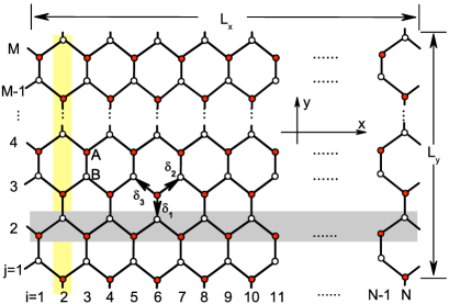
Figure 1: (Color online) Graphene lattice. Lattice sites belonging to the same shaded horizontal or vertical stripes share the same indices $i$ or $j$. The solid circles correspond to the $A$ sublattice and the open circles to the $B$ sublattice. The three nearest neighbor vectors joining the two sublattices are $\bm{\delta}_{k}$, $k=1\ldots 3$.

The Hamiltonian defined on a honeycomb lattice of dimension $L_{x}\times L_{y}$, shown in Fig. 1, is

$$\begin{split}H=&\sum_{\mathbf{n}}[(\epsilon_{\mathbf{n},A}+m)c_{\mathbf{n},A}^{\dagger}c_{\mathbf{n},A}+(\epsilon_{\mathbf{n},B}-m)c_{\mathbf{n},B}^{\dagger}c_{\mathbf{n},B}]\\ &-\sum_{\mathbf{n}}\sum_{k=1}^{3}(t_{\mathbf{n},k}\mathrm{e}^{\mathrm{i}a_{\mathbf{n},k}}c_{\mathbf{n},A}^{\dagger}c_{\mathbf{n+\bm{\delta}}_{k},B}+\mathrm{h.c.}),\end{split}$$ (1)

where the summation of $\mathbf{n}$ ranges over all unit cells, and $c_{\mathbf{n},A}$, $c_{\mathbf{n},B}$ are the fermionic annihilation operators in the unit cell $\mathbf{n}$ for the sublattices $A$ and $B$, respectively. The spacing between vertical slices is $\sqrt{3}a/2$, where $a$ is the bond length. In the transfer matrix calculations $a$ is the unit of length. The size of the sample is chosen such that $L_{x}=N(\sqrt{3}a/2)$ and $L_{y}=M(3a)$, where $N$ is the number of vertical slices and $M$ is the number of unit cells on a vertical slice.

The spin degrees of freedom are omitted, as we assume that the magnetic field is sufficiently strong to completely polarize them. The on-site energies $\epsilon_{\mathbf{n},A}$ and $\epsilon_{\mathbf{n},B}$ are independent random variables. Thus, $V_{\mathbf{n}}=(\epsilon_{\mathbf{n},A}+\epsilon_{\mathbf{n},B})/2$ is a random potential and $M_{\mathbf{n}}=(\epsilon_{\mathbf{n},A}-\epsilon_{\mathbf{n},B})/2$ is mass disorder in the corresponding language of the low energy spectra of Dirac fermions. Here we do not consider mass disorder and therefore choose $\epsilon_{\mathbf{n},A}=\epsilon_{\mathbf{n},B}=V_{\mathbf{n}}$, where $V_{\mathbf{n}}$ is uniformly distributed in the range $[-g_{V}/2,g_{V}/2]$. The mass $m$ provides a charge density modulation between the two sublattices and leads to an energy gap. In the Dirac language this gap would appear as a parity-preserving mass. We choose $t_{\mathbf{n},k}=t+\Delta t_{\mathbf{n},k}$ and set $t=1$, providing a natural energy scale. The quantity $\Delta t_{\mathbf{n},k}$ is a random variable uniformly distributed in the range $[-g_{T}/2,g_{T}/2]$, characterizing the bond disorder. The phases $a_{\mathbf{n},k}$ are such that the magnetic flux per hexagonal plaquette, $\phi$, is $1/Q$, in units of the flux quanta $\phi_{0}=h/e$. We choose a gauge such that $a_{\mathbf{n},1}=\pi i/Q$ for the vertical bonds in slice $i$ as in Fig. 1, and $a_{\mathbf{n},2}=a_{\mathbf{n},3}=0$.

The longitudinal conductance $\sigma_{\mathrm{xx}}$ is studied using the well developed transfer matrix method. Consider a quasi-1D system, $L_{x}\gg L_{y}$ with a periodic boundary condition only along the $y$ direction. Let $\Psi_{i}=(\psi_{i,1},\psi_{i,2},\ldots,\psi_{i,2M})^{T}$ be the amplitudes on the slice $i$ for an eigenstate with a given energy $E$; then amplitudes on the successive slices are related by the matrix multiplication:

$$\left[\begin{array}[]{c}\Psi_{i+1}\\ \Psi_{i}\\ \end{array}\right]=\left[\begin{array}[]{cc}{\cal T}^{-1}_{i}(E-H_{i})&-{\cal T}_{i}^{-1}{\cal T}_{i-1}\\ 1&0\\ \end{array}\right]\left[\begin{array}[]{c}\Psi_{i}\\ \Psi_{i-1}\\ \end{array}\right],$$ (2)

where ${\cal T}_{i}$ is a diagonal matrix with elements $(t_{i,1},t_{i,2},\ldots,t_{i,2M})$ representing the hopping matrix elements connecting the slices $i$ and $i+1$, and $H_{i}$ is the Hamiltonian within the slice. All postive Lyapunov exponents of the transfer matrix Kramer and Schreiber (1996), $\gamma_{1}>\gamma_{2}>\ldots>\gamma_{2M}$, are computed by iterating Eq. (2) and performing frequent orthonormalizations. The convergence of this algorithm is guaranteed by the well known Osledec theorem Oseledec (1968). The conductance per square, $\sigma_{\mathrm{xx}}$, is given by the Landauer formulaFisher and Lee (1981); Baranger and Stone (1989); Kramer and MacKinnon (1993); Sheng and Weng (2000)(note the special factor of $\sqrt{3}$ in the argument of $\cosh$):

$$\sigma_{\mathrm{xx}}=\frac{e^{2}}{h}\sum_{i=1}^{2M}\frac{1}{\cosh^{2}(2\sqrt{3}M\gamma_{i})}.$$ (3)

The localization length in the quasi-1D system of width $L_{y}$ is given by $\lambda_{M}=1/\gamma_{2M}$. Assuming single parameter scaling, $\lambda_{M}/M=f(|E-E_{c}|M^{1/\nu_{\ell}})$, the data collapse yields the critical exponent $\nu_{\ell}$ and the critical energy $E_{c}$.

To compute the Hall conductance $\sigma_{\mathrm{xy}}$, we impose periodic boundary conditions in both directions of the system. The Hamiltonian (1) is diagonalized to obtain a set of energy eigenvalues $E_{\alpha}$ and the corresponding set of eigenstates $|\alpha\rangle$ for $\alpha=1,\ldots,2M\times N$. Then $\sigma_{\mathrm{xy}}$ is computed using the Kubo formula Thouless et al. (1982):

$$\sigma_{\mathrm{xy}}(E)=\frac{ie^{2}\hbar}{L_{x}L_{y}}\sum_{E_{\alpha}<E<E_{\beta}}\frac{\langle\alpha|v_{y}|\beta\rangle\langle\beta|v_{x}|\alpha\rangle-(x\leftrightarrow y)}{(E_{\alpha}-E_{\beta})^{2}},$$ (4)

where $v_{x}=[H,x]/i\hbar$ is the velocity operator along the $x$ direction and similarly for $v_{y}$ in the $y$ direction. Note that the bonds in Fig. 1 that are not parallel to the $y$ direction contribute to both $v_{x}$ and $v_{y}$. The summation corresponds to sum over the states below and above the energy $E$. Finally, the expression is disorder averaged.

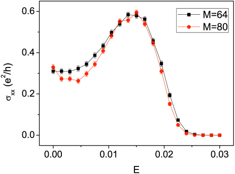
Figure 2: (Color online) The longitudinal conductance $\sigma_{\mathrm{xx}}$ as a function of energy $E$. The magnetic flux through the hexagonal plaquette $\phi=1/200$ and $g_{T}=0.5$.

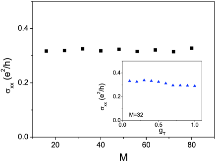
Figure 3: (Color online) Longitudinal conductance $\sigma_{\mathrm{xx}}$ at $E=0$ as a function of the transverse size $M$ for $g_{T}=0.5$ and $g_{V}=0$. The inset shows $\sigma_{\mathrm{xx}}(E=0)$ as a function of $g_{T}$ for $M=32$. The value appears to be independent of $g_{T}$ and close to $\frac{e^{2}}{\pi h}$; the errors bars are about the size of the scatter in the numerical data. The near universality disappears if $g_{V}$ is added.

In the language of Dirac fermions Goswami et al. (2007) random hopping gives rise to both intranode and internode scattering between states on different sublattices. Intranode scattering appears as a random abelian gauge field, and the two inequivalent nodes have opposite charges corresponding to this gauge field. When projected to the lowest Landau level, the abelian gauge field leaves it unaffected. However, the internode scattering mixes the degenerate states corresponding to the two inequivalent nodes and produces extended states at $\pm E_{c}$. The existence of extended states at energies symmetric about $E=0$ is the consequence of the sublattice symmetry of the disorder (often referred to as the chiral or the particle-hole symmetry). It is this special symmetry that leads to a divergent density of states and delocalized states at $E=0$ Goswami et al. (2007); Hikami et al. (1993). However, the calculated finite $\sigma_{xx}$ and a linear variation of $\sigma_{xy}$ with a small slope in the energy range $-E_{c}<E<E_{c}$ hint at the existence of a band of delocalized states between $\pm E_{c}$, as shown below.

In the transfer matrix calculation of $\sigma_{\mathrm{xx}}$ (see Fig. 2), we chose a magnetic field $\phi=1/200$. An iteration of Eq. (2) of the order of $10^{5}$ to $10^{6}$ was performed until the relative errors of less than $0.5\%$ of all the Lyapunov exponents were achieved. The longitudinal conductance $\sigma_{\mathrm{xx}}$ at exactly $E=0$ is computed according to the Landauer formula, Eq. (3), in systems with different values of $M$, as shown in Fig. 3. For only bond disorder, $g_{T}=0.5$, a non-zero longitudinal conductance is observed for all system sizes. The value of $\sigma_{\mathrm{xx}}\sim\frac{e^{2}}{\pi h}$ is found to be independent of $M$ and $g_{T}$. This behavior of $\sigma_{\mathrm{xx}}$ implies an unusual dissipative nature. We have also checked the existence of the dissipative behavior when $g_{v}\neq 0$ in addition.

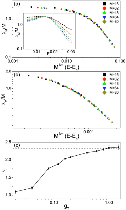
Figure 4: (Color online)(a) Scaling curve for the case $g_{T}=0.5$ and $m=0$. Insert shows the size dependence of the localization length computed in systems with different sizes. (b) Scaling curve for the case $g_{T}=0.2$ and $m=0.2$. (c)The critical exponent $\nu_{\ell}$ as a function of the random hopping intensity $g_{T}$ for $m=0.2$. It varies continuously from $\nu_{\ell}=1.10\pm 0.05$ to $\nu=2.36\pm 0.07$ as the disorder intensity $g_{T}$ is tuned from the weak to strong. The dashed line corresponds to $\nu_{\ell}=7/3$.

To the study of the critical behavior in the presence of bond disorder in the massless case, we set $g_{T}=0.5$. The critical exponent is expected to be independent of the value $g_{T}$ Goswami et al. (2007). The renormalized localization lengths $\lambda_{M}/M$ as a function of $E$ for various $M$ are plotted in in the insert of Fig. 4(a). The critical energy $E_{c}$ is located at a non-zero value $E_{c}=0.0167$ where $\lambda_{M}/M$ is independent of $M$. A successful data collapse based on the data with $E>E_{c}$ leads to a critical exponent of $\nu=2.47\pm 0.04$, close to conventional integer QHE. The scaling form is depicted in Fig. 4(a).

For the massive case, we vary bond disorder with a fixed $m=0.2$ for the purpose of illustration. An example of data collapse is shown in Fig. 4(b) with $g_{T}=0.2$. The critical exponent $\nu_{\ell}=2.08\pm 0.01$ is different from conventional QHE; $\nu_{\ell}$ varies continuously from $1.1\pm 0.05$ to $2.36\pm 0.07$ as the system is tuned from $g_{T}=0.02$ to $g_{T}=1.5$. This behavior agrees with the previous results  Goswami et al. (2007). When $g_{T}\gg m$, the effect of the finite mass is negligible, and the critical exponent of $\nu_{\ell}\approx 7/3$ is recovered, as before.

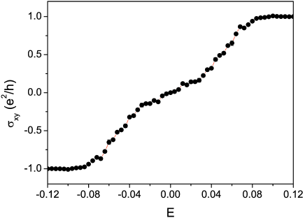
Figure 5: (Color online) Hall conductance $\sigma_{\mathrm{xy}}$ as a function of energy $E$ with bond disorder intensities $g_{T}$. The $\nu=0$ plateau emerges due to the bond disorders.

In computing the energy dependence of $\sigma_{\mathrm{xy}}$ a relatively large flux $\phi=1/20$ is chosen, because smaller values of flux involve many Landau bands in the diagonalization calculations, which are hard to track accurately. The chosen system size was $N=M=40$, and an average over 1000 disorder realizations was performed. The results are shown in Fig. 5. Although there is not a strict plateau at $\nu=0$, there is a break in the slope in the rise between $\nu=-1$ to $\nu=1$, as the energy sweeps past the band center at $E=0$. This can be construed as a plateau-like feature. Since the lowest Landau level splitting is expected to increase with $g_{T}$, so is the extent of the region around $E=0$ with a smaller slope.

The striking results here are the band of extended states in the region $-E_{c}<E<E_{c}$ for bond disorder and the vindication of a continuously varying localization length exponent when, in addition, there is a finite uniform mass present in the Dirac spectrum. The situation is a bit more subtle, however. We had previously observed that the density of states diverges very weakly at $E=0$ Goswami et al. (2007). In particular, for the Lorentzian distribution of disorder this divergence was found to be exactly logarithmic. A $\log^{2}E$ divergence was predicted in Ref. Hikami et al. (1993) for Gaussian disorder corresponding to a Hamiltonian which in fact is formally identical when projected to the lowest Landau level. Such a weak divergence at $E=0$ may give rise to fluctuations responsible for dissipation leading to a finite $\sigma_{\mathrm{xx}}$ Hikami et al. (1993); Ostrovsky et al. (2007). The slightly sloping profile of $\sigma_{\mathrm{xy}}$ centered at $E=0$ is harder to explain analytically. The dissipative behavior at $\nu=0$ is consistent with experiments. However, in contrast to Ref. Abanin et al. (2007), this dissipative behavior is a bulk phenomenon, not an edge phenomenon. It is possible to test this experimentally by varying the aspect ratio of the sample. But we only have a sloping plateau-like feature of $\sigma_{xy}$ at $\nu=0$ unlike Ref. Abanin et al. (2007). It is possible that the difference between the two pictures depends on the relative size of the spin splitting compared to the width of the extended band of states. Clearly further experimental and theoretical work would be very helpful to elucidate the precise nature of this exciting new development.

This work is supported by NSF under Grant No. DMR-0705092. We thank P. A. Lee for valuable comments.

References

- Laughlin (1999) R. B. Laughlin, Rev. Mod. Phys. 71, 863 (1999).
- Novoselov et al. (2005) K. S. Novoselov, A. K. Geim, S. V. Morozov, D. Jiang, M. I. Katsnelson, I. V. Grigorieva, S. V. Dubonos, and A. A. Firsov, Nature 438, 197 (2005).
- Zhang et al. (2005) Y. Zhang, Y.-W. Tan, H. L. Stormer, and P. Kim, Nature 438, 201 (2005).
- Gusynin and Sharapov (2005) V. P. Gusynin and S. G. Sharapov, Phys. Rev. Lett. 95, 146801 (2005).
- Peres et al. (2006) N. M. R. Peres, F. Guinea, and A. H. C. Neto, Phys. Rev. B 73, 125411 (2006).
- Ostrovsky et al. (2007) P. M. Ostrovsky, I. V. Gornyi, and A. D. Mirlin, arXiv:0712.0597v1 (2007).
- Goswami et al. (2007) P. Goswami, X. Jia, and S. Chakravarty, Phys. Rev. B 76, 205408 (2007).
- Koshino and Ando (2007) M. Koshino and T. Ando, Phys. Rev. B 75, 033412 (2007).
- Zhang et al. (2006) Y. Zhang, Z. Jiang, J. P. Small, M. S. Purewal, Y.-W. Tan, M. Fazlollahi, J. D. Chudow, J. A. Jaszczak, H. L. Stormer, and P. Kim, Phys. Rev. Lett. 96, 136806 (2006).
- Abanin et al. (2007) D. A. Abanin, K. S. Novoselov, U. Zeitler, P. A. Lee, A. K. Geim, and L. S. Levitov, Phys. Rev. Lett. 98, 196806 (2007).
- Sheng et al. (2006) D. N. Sheng, L. Sheng, and Z. Y. Weng, Phys. Rev. B 73, 233406 (2006).
- Thouless et al. (1982) D. J. Thouless, M. Kohmoto, M. P. Nightingale, and M. den Nijs, Phys. Rev. Lett. 49, 405 (1982).
- Kramer and Schreiber (1996) B. Kramer and M. Schreiber, in Computational Physics, edited by K. H. Hoffmann and M. Schreiber (Springer, Berlin, 1996), p. 166.
- Oseledec (1968) V. Oseledec, Trans. Moscow Math. Soc. 19, 197 (1968).
- Fisher and Lee (1981) D. S. Fisher and P. A. Lee, Phys. Rev. B 23, 6851 (1981).
- Baranger and Stone (1989) H. U. Baranger and A. D. Stone, Phys. Rev. B 40, 8169 (1989).
- Kramer and MacKinnon (1993) B. Kramer and A. MacKinnon, Rep. Prog. Phys 56, 1469 (1993).
- Sheng and Weng (2000) D. N. Sheng and Z. Y. Weng, Europhys. Lett. 50, 776 (2000).
- Hikami et al. (1993) S. Hikami, M. Shirai, and F. Wegner, Nucl. Phys. B 408, 415 (1993).