Multiscale Edge Detection in the Corona

Abstract

Coronal Mass Ejections ( CMEs ) are challenging objects to detect using automated techniques, due to their high velocity and diffuse, irregular morphology. A necessary step to automating the detection process is to first remove the subjectivity introduced by the observer used in the current, standard, CME detection and tracking method. Here we describe and demonstrate a multiscale edge detection technique that addresses this step and could serve as one part of an automated CME detection system. This method provides a way to objectively define a CME front with associated error estimates. These fronts can then be used to extract CME morphology and kinematics. We apply this technique to a CME observed on 18 April 2000 by the Large Angle Solar COronagraph experiment ( LASCO ) C2/C3 and a CME observed on 21 April 2002 by LASCO C2/C3 and the Transition Region and Coronal Explorer ( TRACE ). For the two examples in this work, the heights determined by the standard manual method are larger than those determined with the multiscale method by $\approx{10}\%$ using LASCO data and $\approx{20}\%$ using TRACE data.

1 Introduction

Currently, the standard method for detection and tracking of Coronal Mass Ejections ( CMEs ) is by visual inspection (e.g., the CUA CDAW CME catalog, available at http://cdaw.gsfc.nasa.gov). A human operator uses a sequence of images to visually locate a CME. A feature of interest is marked interactively so that it may be tracked in the sequence of images. From these manual measurements, the observer can then plot height–time profiles of the CMEs. These height measurements are used to compute velocities and accelerations (e.g., gallagher03). Although the human visual system is very sensitive, there are many problems with this technique. This methodology is inherently subjective and prone to error. Both the detection and tracking of a CME is dependent upon the experience, skill, and well being of the operator. Which object, or part of the CME to track varies, from observer to observer and is highly dependent on the quality of the data. Also, there is no way to obtain statistical uncertainties, which is particularly important for the determination of velocity and acceleration profiles. Lastly, the inability to handle large data volumes and the use of an interactive, manual analysis do not allow for a real-time data analysis required for space weather forecasting. A visual analysis of coronagraph data is a tedious and labor-intensive task. Current data rates from the Solar and Heliospheric Observatory ( SOHO ) are low enough to make an interactive analysis possible (${<}$1 Gigabyte/day). This will not be the case for recent missions such as the Solar TErrestrial RElations Observatory ( STEREO ) and new missions such as the Solar Dynamics Observatory ( SDO ). These missions have projected data rates that make an interactive analysis infeasible ($>$1 Terabyte/day). For these reasons, it is necessary to develop an automatic, real-time CME detection and tracking system. Current digital imaging processing methods and paradigms provide the tools needed for such a system. In the next section we discuss in general, the parts needed in an automated system, as well as some of the current work on this topic.

2 A System for Automatic CME Detection

The general design for an automated CME detection system should basically follow the digital image-processing paradigm described by gonzalez02. Digital image processing as they describe can basically be broken into three parts: i) image preprocessing and segmentation; ii) image representation and description, and; iii) object recognition. Image preprocessing includes standard image preparation such as calibration, cosmic ray removal but it also includes noise reduction based on the statistics of the image (e.g., Gaussian or Poisson; starck02). Image segmentation is the extraction of individual features of interest in an image (e.g., edges, boundaries, and regions). Some methods used for this part include filtering, edge detection, and morphological operations. Image representation and description converts the extracted features into a form such as statistical moments or topological descriptors (e.g., areas, lengths, etc.) that are easier to store and manipulate computationally. Object recognition includes techniques such as neural networks and support vector machines ( SVMs ) to characterize and classify descriptors determined in the previous step.

Determining the complex structure of CMEs is complicated by the fact that CMEs are diffuse objects with ill-defined boundaries, making their automatic detection with many traditional image processing techniques a difficult task. To address this difficulty, new image processing methods were employed by stenborg03 and portier01, who were the first to apply a wavelet-based technique to study the multiscale nature of coronal structures in LASCO and EIT data, respectively. Their methods employed a multilevel decomposition scheme via the so-called “à trous” wavelet transform.

robbrecht04, developed a system to autonomously detect CMEs in image sequences from LASCO. Their software, Computer Aided CME Tracking ( CACTus )(http://sidc.oma.be/cactus/), relies on the detection of bright ridges in CME height–time maps using the Hough transform. The main limitation of this method is that the Hough transform (as implemented) imposes a linear height–time evolution, therefore forcing constant velocity profiles for each bright feature. This method is therefore not appropriate to study CME acceleration. Other autonomous CME detection systems include ARTEMIS [Boursier et al. (2005)] (http://lascor.oamp.fr/lasco/index.jsp), the Solar Eruptive Event Detection Systems ( SEEDS )[Olmedo et al. (2005)] (http://spaceweather.gmu.edu/seeds/), and the Solar Feature Monitor [Qu et al. (2006)] (http://filament.njit.edu/detection/vso.html).

In this work, a multiscale edge detector is used to objectively identify and track CME leading edges. In Section 3, Transition Region and Coronal Explorer ( TRACE; handy99 ) and Large Angle and Spectrometric COronagraph experiment ( SOHO/LASCO; brueckner95 ) observations and initial data-reduction is discussed, while the multiscale-based edge detection techniques are presented in Section 4. Our results and conclusions are then given in Sections 5 and 6.

3 Observations

To demonstrate the use of multiscale edge detection on CMEs in EUV imaging and white-light coronagraph, data two data sets were used. The first data set contains a CME observed on 18 April 2000 with the LASCO C2 and C3 telescopes. The data set contains six C2 images and two C3 images. The second data set of TRACE and LASCO observations contains a CME observed on 21 April 2002. The data set contains one C2 image, three C3 images, and 30 TRACE images. TRACE observed a very faint loop-like system propagating away from the initial flare brightening, which was similar in shape to a CME (or number of CMEs) observed in LASCO. The appearance of the features remained relatively constant as they passed through the TRACE 195 Å passband and LASCO fields of view.

The TRACE observations were taken during a standard 195 Å bandpass observing campaign that provides 20 second cadence and an image scale of 0.5 arcsec per pixel. Following gallagher02b, standard image corrections were first applied before pointing offsets were accounted for by cross-correlating and shifting each frame. The white-light LASCO images were obtained using a standard LASCO observing sequence. The C2 images were taken using the orange filter (5400 – 6400 Å) with a variable cadence between 16 and 37 minutes and an image scale of 11.9 arcsec per pixel. The C3 images were taken using the clear filter (4000 – 8500 Å) with a variable cadence between 24 and 60 minutes and an image scale of 56 arcsec per pixel. Both the C2 and C3 images were unpolarized. Table 1 summarizes the details of these two data sets.

Table 1.: Data sets for the 18 April 2000 and 21 April 2002 CMEs used in this work.

	18 April 2000		21 April 2002
	C2	C3	C2	C3	TRACE
Start time (UT)	16:06	17:18	01:27	01:42	00:46
Wavelength (Å)	5400 – 6400	4000 – 8500	5400 – 6400	4000 – 8500	195
no. images	6	2	1	3	30
pix. size (arcsec)	11.9	56	11.9	56	0.5
min/max cadence	16/37 min	24/60 min	16/37 min	24/60 min	20 sec

4 Methodology

4.1 Edge Detection

Sharp variations or discontinuities often carry the most important information in signals and images. In images, these take the form of boundaries described by edges that can be detected by taking first and second derivatives [Marr (1982)]. The most common choice of first derivative for images is the gradient [Gonzalez and Woods (2002)]. The gradient of an image $I(x,y)$ at a point $(x,y)$ is the vector,

$${\bf\nabla}{I}(x,y)=\left(\begin{array}[]{c}\frac{\partial{I}}{\partial{x}}\\ \frac{\partial{I}}{\partial{y}}\end{array}\right)=\left(\begin{array}[]{c}G_{x}\\ G_{y}\end{array}\right).$$ (1)

The gradient points in the direction of maximum change of $I$ at $(x,y)$. The magnitude of this change is defined by the magnitude of the gradient,

$$|{\bf\nabla}{I}(x,y)|=(G_{x}^{2}+G_{y}^{2})^{1/2}.$$ (2)

The direction of the change at $(x,y)$ measured with respect to the $x$-axis is,

$$\alpha(x,y)=\arctan(G_{x}/G_{y}).$$ (3)

The edge direction is perpendicular to the gradient’s direction at $(x,y)$.

The partial derivatives $G_{x}$ and $G_{y}$ are well approximated by the Sobel and Roberts gradient operators [Gonzalez and Woods (2002)], although these operators cannot easily be adapted to multiscale applications. In this work, scale is considered to be the size of the neighborhood over which the changes are calculated.

  

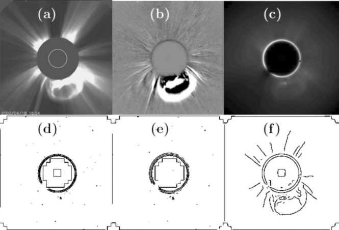
Figure 1.: (a) A LASCO C2 image of a 18 April 2000 CME at 16:54 UT processed with a monthly background model. (b) A running-difference image made by subtracting the previous C2 image from the 16:54 UT image. (c) The unprocessed C2 image. (d) Edges from applying the Roberts edge detector to the unprocessed image. (e) Edges from applying the Sobel edge detector to the unprocessed image. (f) Edges from applying the Canny edge detector ($\sigma=5$) to the unprocessed image.

Most edges are not steep, so additional information to that returned by the gradient is needed to accurately describe edge properties. This can be achieved using multiscale techniques. First proposed by canny86, this form of edge detection uses Gaussians of different width ($\sigma$) as a smoothing operator $\theta_{\sigma}$. The Gaussians are convolved with the original image, so that Gaussians with smaller width correspond to smaller length-scales. Equation (1) for the Canny edge detector can be written as,

$$\nabla{(\theta_{\sigma}{\ast}I(x,y))}=\left(\begin{array}[]{c}\frac{\partial{}}{\partial{x}}{(\theta_{\sigma}{\ast}I(x,y))}\\ \frac{\partial{}}{\partial{y}}{(\theta_{\sigma}{\ast}I(x,y))}\end{array}\right).$$ (4)

The image is smoothed using a Gaussian filter with a selected ${\sigma}$. Then a derivative of the smoothed image is computed for the $x$ and $y$-directions. The local gradient magnitude and direction are computed at each point in the image. An edge point is defined as a point whose gradient-magnitude is locally maximum in the direction defined by ${\alpha}$. These edge points form ridges in the gradient magnitude image. The process of non-maximal suppression is performed by setting to zero all pixels not lying along the ridges. The ridge pixels are then thresholded using two thresholds ($T_{a}$ and $T_{b}$ with $T_{b}>T_{a}$). Ridge pixels with values between $T_{a}$ and $T_{b}$ are defined as weak edges. The ridge pixels with values greater than $T_{b}$ are called strong edges. The edges are linked by incorporating the weak edges that are 8-connected with the strong pixels [Gonzalez and Woods (2002)]. Figure 1 shows a comparison of the Roberts, Sobel, and Canny edge detectors applied to an unprocessed LASCO C2 image of the 18 April 2000 CME from 16:54 UT. The Roberts (Figure 1(d)) and the Sobel (Figure 1(e)) detectors pick up a small piece of the CME core and noise. Using the multiscale nature of the Canny detector (Figure 1(f)), choosing a larger scale size ($\sigma=5$), edges corresponding to streamers and the CME front can be seen. Unfortunately, the Canny method has two main limitations: i) it is slow because it is based on a continuous transform and, ii) there is no natural way to select appropriate scales.

4.2 Multiscale Edge Detection

mallat92a, showed that the maximum modulus of the continuous wavelet transform ( MMWT ) is equivalent to the multiscale Canny edge detector described in the previous section. The wavelet transform converts a 2D image into a 3D function, where two of the dimensions are position parameters and the third dimension is scale. The transform decomposes the image into translated and dilated (scaled) versions of a basic function called a wavelet: $\psi(x,y)$. A wavelet dilated by a scale factor $s$ is denoted as

$$\psi_{s}(x,y)=\frac{1}{s^{2}}\psi(\frac{x}{s},\frac{y}{s})={s^{-2}}\psi({s^{-1}}{x},{s^{-1}}{y}).$$ (5)

The wavelet is a function that satisfies a specific set of conditions, but these functions have the key characteristic that they are localized in position and scale [Mallat (1998)]. The minimum and maximum scales are determined by the wavelet transform, addressing the first problem of the Canny edge detector mentioned in the previous section.

mallat92b refined the wavelet transform describe by Mallat and Hwang, creating a fast, discrete transform. This addresses the computational speed problem of the Canny edge detector making this fast transform more suited to realtime applications. As with the Canny edge detector, this wavelet starts with a smoothing function: ${s^{-2}}\theta({s^{-1}}{x},{s^{-1}}{y})$. The smoothing function is a cubic spline, a discrete approximation of a Gaussian. The smoothing function is also separable, i.e. $\theta(x,y)=\theta(x)\theta(y)$. The wavelets are then the first derivative of the smoothing function. This allows the wavelets to be written as

$$\psi_{s}^{x}(x,y)={s^{-2}}\frac{\partial\theta({s^{-1}}x)}{\partial{x}}{\theta({s^{-1}}y)}\mbox{ and }\psi_{s}^{y}(x,y)={{s^{-2}}\theta({s^{-1}}x)}\frac{\partial\theta({s^{-1}}y)}{\partial{y}}.$$ (6)

Another factor that adds to the speed of the wavelet transform algorithm is the choice of a dyadic scale factor ($s$). Dyadic means that $s=2^{j}$ where $j=1,2,{\ldots},J$ or $s=2^{1},2^{2},2^{4},2^{8},{\ldots},2^{J}$, smallest scale to largest scale. The index $J$ is determined by the largest dimension of the image, $N$, i.e., $N=2^{J}$. The wavelet transforms of $I(x,y)$ with respect to $x$ and $y$ at scale s can then be written

$$\begin{array}[]{c}W_{s}^{x}I=W_{s}^{x}I(x,y)=\psi_{s}^{x}(x,y)\ast I(x,y)\\ \mbox{and}\\ W_{s}^{y}I=W_{s}^{y}I(x,y)=\psi_{s}^{y}(x,y)\ast I(x,y),\end{array}$$ (7)

where $\ast$ denotes a convolution. Substituting these into Equations (2) and (3) gives the following expression for the gradient of an image at scale s in terms of the wavelets:

$$\begin{array}[]{c}|\nabla_{s}{I}(x,y)|=((W_{s}^{x}I)^{2}+(W_{s}^{y}I)^{2})^{1/2}\\ \mbox{and}\\ \alpha_{s}(x,y)=\arctan(W_{s}^{x}I/W_{s}^{y}I).\end{array}$$ (8)

The detailed steps associated with implementing Equation (6) are shown in Figure 2. The rows from top to bottom are scales one to five, respectively. Column (a) displays the horizontal wavelet components $W_{s}^{x}I(x,y)$. Column (b) shows the vertical wavelet components $W_{s}^{y}I(x,y)$. The next two columns show the magnitude (c) of the multiscale gradient and the angle (d) of the multiscale gradient. The edges calculated from the multiscale gradient are displayed in column (e).

  

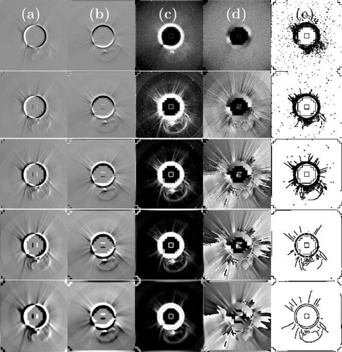
Figure 2.: The steps calculating the multiscale edges of the unprocessed C2 image (18 April 2000 CME at 16:54 UT). The rows from top to bottom are scales $j=1$ to $j=5$ respectively. (a) Horizontal wavelet coefficients. (b) Vertical wavelet coefficients. (c) The magnitude of the multiscale gradient. (d) The angle of the multiscale gradient. (e) The edges calculated from the multiscale gradient.

4.3 Edge Selection and Error Estimation

Once the gradient was found using the wavelet transform, the edges were calculated using the local maxima at each scale, as described in the end of Section 4.1. Closed or stationary edges due to features such as coronal loops, ribbons, and cosmic rays were then removed, thus leaving only moving, open edges visible. Currently not all available information is used so there were still some open spurious edges that were removed manually. Finally, only the edges from expanding, moving features were left. It was these edges that were used to characterize the temporal evolution of the CME front.

The multiscale edge detector can objectively define the CME front but it is also important to estimate the statistical uncertainty in the edges and to obtain errors in position or height. A straightforward way to do this is by using a bootstrap (efron93). To do this we must create statistical realizations of the data, then apply the multiscale edge detection method to each realization. The realizations of the data are created by estimating a true, non-noisy image then applying a noise model to the true image. Applying the noise model means using a random number generator (random deviate) for our particular noise model to generate noise and adding to the non-noisy image estimate. In our case the noise model is well approximated by Gaussian noise. Estimation of the noise and the true image is described by starck02. The noise model is applied 1000 times to the true image with each application creating a new realization. Doing this 1000 times, a mean and standard deviation is calculated for the edge location or in our case for each height point used. The steps for creating the estimate are i) estimate the noise in the original image, ii) compute the isotropic wavelet transform of the image (à trous wavelet transform), iii) threshold the wavelet coefficients based on the estimated noise, and iv) reconstruct the image. The reconstructed image is the estimate of the true image. The noise estimate from the original image is used in the noise model applied to the estimated true image.

5 Results

  

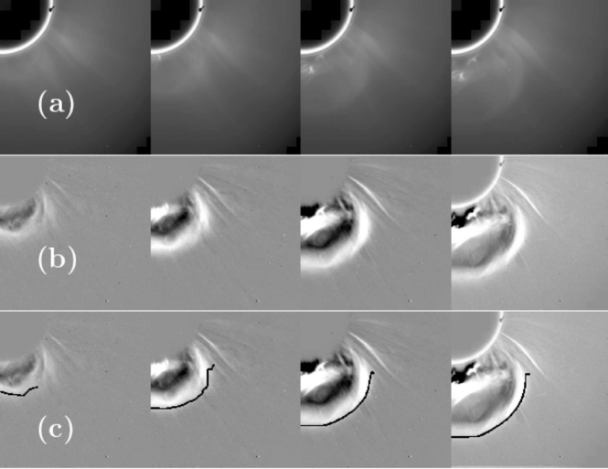
Figure 3.: Illustration of a CME edge detection in subsequent images. (a) The original LASCO C2 images, (b) running difference images of the LASCO C2 images, and (c) application of the multiscale edge detection algorithm to the sequence of the original images. The edges are the black lines displayed over the running difference images. The CME erupted on 18 April 2000, the times for the frames are (from left to right) 16:06 UT, 16:30 UT, 16:54 UT, and 17:06 UT.

The first example of application of the multiscale edge detection is illustrated in Figure 3. Figure 3(a) shows four of the original, unprocessed LASCO C2 images for the 18 April 2000 data set. The times for the frames from left to right are 16:06 UT, 16:30 UT, 16:54 UT, and 17:06 UT. Figure 3(b) shows running difference images for the sequence of C2 images. The results of the multiscale edge detection method applied to the original images are shown in Figure 3(c). The edges of the CME front are displayed as black contours over the difference images shown in Figure 3(b). Once the method is applied to the entire data set of C2 and C3 images, one point from each edge (all at the same polar angle) is selected. The distance of each point from Sun center is plotted against time to create a height-time profile. A bootstrap (described in Section  4.3) was performed for each edge calculation so that each point in the height–time profile has an associated error in height.

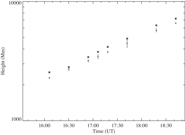
Figure 4.: The height–time profile for the 18 April 2000 CME. The data plotted using + symbols were obtained via the multiscale methods described herein, while the data plotted using $\ast$ symbols are from the CU CDAW CME catalog. The first six points are for LASCO C2 and the last two are for LASCO C3.

The resulting height–time profile is shown in Figure 4. The data plotted using + symbols are those obtained via the multiscale method. One-${\sigma}$ errors in height are also shown. For comparison, data from the CUA CDAW CME catalog are plotted in the figure using $\ast$ symbols. The points determined with the multiscale method are systematically lower in height than the points from the CUA CDAW points. This is because the CUA CDAW points are selected using difference images and, as can be seen in Figure 3(c), the true CME front (black edge) is inside of the edge in the difference images. This illustrates a drawback of using difference images to determine the CME front. The difference image height estimates from the CUA CDAW catalog are larger than the multiscale edge estimates by $\approx{10}\%$.

  

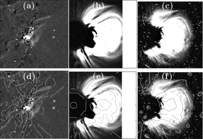
Figure 5.: (a) TRACE 195 Å difference image from 21 April 2002, created by subtracting an image taken at 00:43:10 UT from an image at 00:42:30 UT, together with running difference images from (b) LASCO C2 (01:50:05 UT) and (c) LASCO C3 (02:13:05 UT). The same (d) TRACE and (e,f) LASCO images (as shown in (a), (b), and (c) respectively, but now overlaid with multiscale edges from a scale ($j=8$) that isolates the leading-edge of the CME. (The C2 images are not cut off on the right side. In order for the C2 images to have a similar FOV as the C3 images and for all images to be square, white space was added to the C2 images.)

Figure 5 displays data from the 21 April 2002 data set. Figure 5(a) shows a TRACE difference image created by subtracting an image at 00:42:30 UT from an image at 00:43:10 UT. A very faint loop-like feature was only visible in the difference image after it was smoothed and scaled to an extremely narrow range of intensities. Both these operations were arbitrarily decided upon, and are therefore likely to lead to the object’s true morphology being distorted. Figure 5(d) shows the same TRACE difference image as Figure 5(a) but overlaid with multiscale edges at scale $j=8$. The edge of the faint loop-like features is clearly visible as a result of decomposing the image using wavelets, and then searching for edges in the resulting scale maps using the gradient-based techniques described in the previous section. Figures 5(b) and 5(c) show LASCO C2 and C3 running difference images, respectively. Figures 5(e) and 5(f) show the LASCO difference images overlaid with the multiscale edges for scale $j=8$.

  

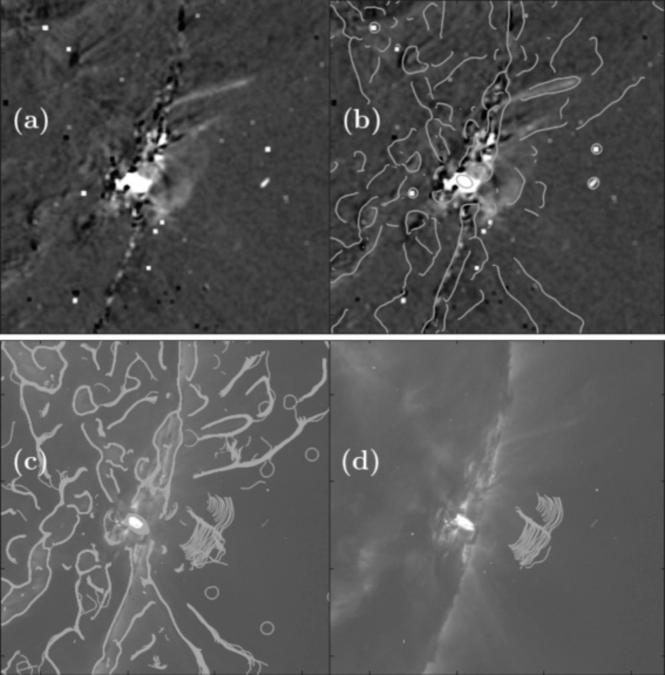
Figure 6.: (a) TRACE 195 Å difference image from 21 April 2002, created by subtracting an image taken at 00:43:10 UT from an image at 00:42:30 UT. (b) The same TRACE images, but now overlaid with multiscale edges from a scale ($j=8$) that isolates the leading-edge of the CME. (c) The set of multiscale edges at scale $j=8$, from all 30 TRACE images (00:46:34 UT to 01:05:19 UT) superimposed on the first image of the TRACE sequence. (d) Same as Figure 6(c), but with unwanted edges removed.

Figure 6 displays on the TRACE data for the 21 April 2002 data set. Figure 6(a) displays the processed difference image (same as Figure 5(a)) and Figure 6(b) is the difference image overlaid with multiscale edges at scale $j=8$ (same as Figure 5(d)). The underlying TRACE image in Figure 6(c) is the original image from 00:46:34 UT. The multiscale edges at scale $j=8$ were calculated for all 30 TRACE images from 00:46:34 UT to 01:05:19 UT. All 30 sets of edges were overlaid upon the original base image. Figure 6(d) contains the same set of edges but by using size and shape information, the expanding front is isolated. The leading edge, only partially visible in the original TRACE difference image in Figure 6(a), is now clearly visible and therefore more straightforward to characterize in terms of its morphology and kinematics. The multiscale edges reveal the existence of two separate moving features.

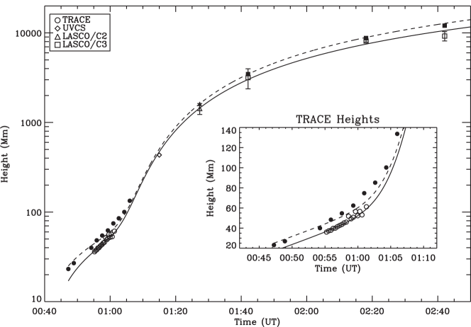
Figure 7.: The height–time profile for the 21 April 2002 CME, together with fits assuming an exponential acceleration of the form given in Equation (9). The data plotted using open symbols were obtained via the multiscale methods described here, while the data plotted using solid symbols are from Gallagher, Lawrence, and Dennis (2003). The solid line is a fit to the multiscale data, the dashed to the latter. Error bars on the LASCO data have been multiplied by a factor of two to improve their visibility and the mean uncertainty in TRACE-derived heights are equal to the diameter of the open and filled circles ($\approx$3 Mm).

Using these edges, the expansion and motion of the CME from the sun is now clearly visible and therefore characterizing it in terms of its morphology and kinematics is more straightforward. The resulting height–time plot is show in Figure 7, together with data from gallagher03, for comparison. We again find the heights determined manually are larger by $\approx{10}\%$ using LASCO data and $\approx{20}\%$ using TRACE data.

Following a procedure similar to that of Gallagher, Lawrence, and Dennis, the height-time curve was fitted assuming a double exponential acceleration profile of the form:

$$a(t)=\left(\frac{1}{a_{r}\exp{(t/\tau_{r})}}+\frac{1}{a_{d}\exp{(-t/\tau_{d})}}\right)^{-1},$$ (9)

where $a_{r}$ and $a_{d}$ are the initial accelerations and $\tau_{r}$ and $\tau_{d}$ give the e-folding times for the rise and decay phases. A best fit to the height–time curve was obtained with $h_{0}=17\pm 3$ Mm, $v_{0}=40\pm 4$ km s^-1, $a_{r}=1\pm 1$ m s^-2, $\tau_{r}=138\pm 26$ s, $a_{d}=4950\pm 926$ m s^-2, and $\tau_{d}=1100\pm 122$ s, and is shown in Figure 7.

6 Conclusions and Future Work

CMEs are diffuse, ill-defined features that propagate through the solar corona and inner heliosphere at large velocities $(\geq$100 km s${}^{-1})$ [Yashiro et al. (2004)], making their detection and characterization a difficult task. Multiscale methods offer a powerful technique by which CMEs can be automatically identified and characterized in terms of their shape, size, velocity, and acceleration.

Here, the entire leading edge of the 18 April 2000 and 21 April 2002 CMEs has been objectively identified and tracked using a combination of wavelet and gradient based techniques. We have shown that multiscale edge detection successfully locates the front edge for both well-defined events seen in LASCO as well as very faint structures seen in TRACE. Although height–time profiles were only calculated for one point, this method allows us to objectively calculate height–time profiles for the entire edge. This represents an advancement over previous point-and-click or difference-based methods, which only facilitate the CME apex to be tracked. Comparing height–time profiles determined using standard methods with the multiscale method shows that for these two CMEs the heights determined manually are larger by $\approx{10}\%$ using LASCO data and $\approx{20}\%$ using TRACE data.

Future work is needed to fully test the use of this technique in an automated system. Application of this edge detection method to a large, diverse set of events is necessary. An important improvement would be better edge selection. This will be accomplished by better incorporating scale information. By chaining the edges together as a function of scale we can distinguish false edges from true edges. This information can also be used to better distinguish better different-shaped edges. Another improvement can be made by using image enhancement. During the denoising stage, wavelet-based image enhancement (such as in stenborg03) can be performed at the same time that noise in the images is estimated and reduced. More sophisticated multiscale methods using transforms such as curvelets will be studied. In order to distinguish between edges such as those due to streamers from those due to a CME front angle information can be incorporated. This multiscale edge detection has been shown to have potential as a useful tool for studying the structure and dynamics of CMEs. With a few more improvements this method could prove to be an important part of an automated system.

Acknowledgements

The authors thank the referee for their suggestions and comments and NASA for its support. CAY is supported by the NASA SESDA contract. PTG is supported by a grant from Science Foundation Ireland’s Research Frontiers Programme.

References

- Boursier et al. (2005) Boursier, Y., Llebaria, A., Goudail, F., Lamy, P., Robelus, S.: 2005, Automatic detection of coronal mass ejections on LASCO-C2 synoptic maps. SPIE 5901, 13-24.
- Brueckner et al. (1995) Brueckner, G.E., Howard, R.A., Koomen, M.J., Korendyke, C.M., Michels, D.J., Moses, J.D., Socker, D.G., Dere, K.P., Lamy, P.L., Llebaria, A., Bout, M.V., Schwenn, R., Simnett, G.M., Bedford, D.K., Eyles, C.J.: 1995, The Large Angle Spectroscopic Coronagraph (LASCO). Sol. Phys., 162, 357-402.
- Canny (1986) Canny, J.: 1986, A computational approach to edge detection. IEEE Trans. Patt. Recog. Mach. Intell. 8, 679-698.
- Efron and Tibshirani (1993) Efron, S., Tibshirani, R.J.: 1993, An Introduction to the Bootstrap, Chapman and Hall, New York.
- Gallagher, Lawrence, and Dennis (2003) Gallagher, P.T., Lawrence, G.R., Dennis, B.R.: 2003, Rapid Acceleration of a Coronal Mass Ejection in the Low Corona and Implications for Propagation. ApJ, 588, L53-L56.
- Gallagher et al. (2002) Gallagher, P.T., Dennis, B.R., Krucker, S., Schwartz, R.A., Tolbert, A.K.: 2002, RHESSI and TRACE Observations of the 21 April 2002 X1.5 Flare. Sol. Phys., 210, 341-356.
- Gonzalez and Woods (2002) Gonzalez, R.C., Woods, R.E.: 2002, Digital Image Processing: Second Edition, Prentice-Hall, Upper Sandle River
- Handy et al. (1999) Handy, B.N., Acton, L.W., Kankelborg, C.C., Wolfson, C.J., Akin, D.J., Bruner, M.E., Caravalho, R., Catura, R.C., Chevalier, R., Duncan, D.W., Edwards, C.G., Feinstein, C.N., Freeland, S.L., Friedlaender, F.M., Hoffmann, C.H., Hurlburt, N.E., Jurcevich, B.K., Katz, N.L., Kelly, G.A., Lemen, J.R., Levay, M., Lindgren, R.W., Mathur, D.P., Meyer, S.B., Morrison, S.J., Morrison, M.D., Nightingale, R.W., Pope, T.P., Rehse, R.A., Schrijver, C.J., Shine, R.A., Shing, L., Strong, K.T., Tarbell, T.D., Title, A.M., Torgerson, D.D., Golub, L., Bookbinder, J.A., Caldwell, D., Cheimets, P.N., Davis, W.N., Deluca, E.E., McMullen, R.A., Warren, H.P., Amato, D., Fisher, R., Maldonado, H., Parkinson, C.: 1999, The transition region and coronal explorer. Sol. Phys., 187, 229-260.
- Mallat (1998) Mallat, S.: 1998, A Wavelet Tour of Signal Processing, AP Press, San Diego.
- Mallat and Hwang (1992) Mallat, S., Hwang, W.L.: 1992, Singularity detection and processing with wavelets. IEEE Trans. Inform. Theory 38, 617-643.
- Mallat and Zhong (1992) Mallat, S., and Zhong, S. 1992, Characterization of signals from multiscale edges. IEEE Trans. Patt. Anal. Mach. Intell., 14, 710-732.
- Marr (1982) Marr, D. 1982, Vision, W.H. Freeman and Company, New York.
- Olmedo et al. (2005) Olmedo, O., Zhang, J., Wechsler, H., Borne, K., Poland, A.: 2005, Solar Eruptive Event Detection System (SEEDS). Bull. Am Astron. Soc. 37, 1342.
- Portier-Fozzani et al. (2001) Portier-Fozzani, F., Vandame, B., Bijaoui, A., Maucherat, A.J.: 2001, A Multiscale Vision Model applied to analyze EIT images of the solar corona. Sol. Phys., 201, 271-287.
- Qu et al. (2006) Qu, M., Shih, F.Y., Jing, J., Wang, H.: 2006, Automatic Detection and Classification of Coronal Mass Ejections. Sol. Phys.. 237, 419-431.
- Robbrecht and Berghmans (2004) Robbrecht, E., Berghmans, D.: 2004, Automated recognition of coronal mass ejections (CMEs) in near-real-time data. A&A, 425, 1097 - 1106.
- Starck and Murtagh (2002) Starck, J.-L., Murtagh, F. 2002, Handbook of Astronomical Data Analysis, Springer Verlag, Berlin.
- Stenborg and Cobelli (2003) Stenborg, G., Cobelli, P.J.: 2003, A wavelet packets equalization technique to reveal the multiple spatial-scale nature of coronal structures. A&A, 398, 1185-1193.
- Yashiro et al. (2004) Yashiro, S., Gopalswamy, N., Michalek, G., St. Cyr, O.C., Plunkett, S.P., Rich, N.B., Howard, R.A., 2004, A catalog of white light coronal mass ejections observed by the SOHO spacecraft. J. Geophys. Res., 109(A7), A07105.