Limits of the Plane Wave Approximation in the Measurement of Molecular Properties

Abstract

Rescattering electrons offer great potential as probes of molecular properties on ultrafast timescales. The most famous example is molecular tomography, in which high harmonic spectra of oriented molecules are mapped to “tomographic images” of the relevant molecular orbitals. The accuracy of such reconstructions may be greatly affected by the distortion of scattering wavefunctions from their asymptotic forms due to interactions with the parent ion. We investigate the validity of the commonly used plane wave approximation in molecular tomography, showing how such distortions affect the resulting orbital reconstructions.

When atoms or molecules are subjected to the field of an intense laser, they may experience loss of electrons through tunnel ionization. The freed electrons may then propagate in the laser field and reencounter the parent ion. This rescattering process has been observed to produce high harmonic generation, above threshold ionization, nonsequential double ionization, etc., depending on which scattering channel an experiment chooses to monitor. [1, 2] Recently, rescattering experiments, as well as their time reversed photoionization counterparts, have received much attention as probes of molecular properties on ultrafast timescales [3, 4, 5]. The best known such technique is molecular tomography[6], which uses high harmonic spectra from aligned molecules to reconstruct molecular wavefunctions.

Rescattering electrons offer clear advantages as probes of molecular structure. The intrinsic timescale of an ionization-acceleration-rescattering process is on the order of a single half-cycle of the driving laser field, typically a few fs. Because the liberated electron is accelerated by the driving laser field, simple formulas arising from classical physics are sufficient to map the energy of a rescattering event to the instants in a laser half-cycle when the electron is liberated and returns, allowing time resolutions to be pushed to the the sub-fs level. Interactions between electronic and vibrational degrees of freedom permit the evolving vibrational states of the parent molecule to be probed [7].

All of these techniques rely on the same underlying physical process, in which the rescattering electron interacts with the parent ion. Thus, such measurements of molecular properties are inherently limited by the degree to which this rescattering is understood. However, to date most efforts to measure molecular properties have treated the rescattering wavefunction as a free electron plane wave, unperturbed by the electron interaction with the parent ion. Prior work relating to such reconstructions has dealt with bandwidth limitations arising from the HHG spectrum [8], orthogonality of the scattering- and bound-state wavefunctions [9, 10], and perturbative treatments of the ionic Coulomb potential [11]. This paper investigates the departure from plane wave scattering which is caused by a nonzero molecular potential and the implications of that departure for molecular tomography. “Tomographic images” of bound states are calculated for a one dimensional square well, and for two molecules in three dimensions, $N_{2}$ and $F_{2}$.

1 Scattering States and Ramifications for Molecular Tomography

At its heart, the tomographic procedure attempts to measure the dipole matrix element

$$\vec{d}_{\vec{k}}=\int d^{3}\vec{x}\psi_{\vec{k}}(\vec{x})\vec{x}\psi_{g}(\vec{x})$$ (1)

in momentum space between a continuum wavefunction $\psi_{\vec{k}}(\vec{x})$ which asymptotically goes as $e^{i\vec{k}\cdot\vec{x}}$ and a particular orbital $\psi_{g}(\vec{x})$ of some target molecule. In the limit where the molecular potential is zero, the plane wave approximation for the scattering states would be exact, and the wavefunction could be reconstructed according to

$$\vec{x}\psi_{g}(\vec{x})=\int d^{3}\vec{k}e^{-i\vec{k}\cdot\vec{x}}\vec{d}_{k}(\vec{x})$$ (2)

A nonzero molecular potential complicates this picture. In one dimension, the WKB approximation gives the continuum scattering state as

$$\psi_{c}\propto\frac{1}{\sqrt{k(x)}}e^{i\int^{x}k(x^{\prime})dx^{\prime}}$$ (3)

where $k(x)=\sqrt{2(E-V(x))}$. In the vicinity of the molecule, both the amplitude and the phase of the scattering state depart from the plane wave approximation.

An ideal tomographic experiment would measure $\vec{d}_{\vec{k}}$ between continuum states and an unperturbed molecular ion. In contrast, in rescattering experiments, recombination occurs in the presence of a strong and time-varying external laser field. The magnitude of the incoming wavefunction is affected by tunnel ionization from the molecular HOMO and the propagation of the electron between ionization and recombination. In addition, the high harmonic spectrum is sharply peaked at frequencies which are multiples of the driving laser frequency. For these reasons, it would be very appealing to measure $\vec{d}_{\vec{k}}$ using photoionization rather than high harmonic generation [9]. It is not clear how the phase of $\vec{d}_{\vec{k}}$ would be measured in such an experiment, but it is at least conceivable to do so by introducing some kind of interfering pathways. However, since this paper is concerned with the limitations to tomographic reconstruction under ideal circumstances, we henceforth assume that such photoionization amplitudes $\vec{d}_{\vec{k}}$ could in principle be found. The issues discussed here with respect to tomographic reconstruction for a photoionization experiment apply also to HHG tomography, with the stipulation that the relevant scattering states should be calculated in the presence of an external laser field in order to provide an exact description.

Problems with the tomographic reconstruction procedure arise when the scattering states $\psi_{\vec{k}}(\vec{x})$ begin to deviate from the plane waves that were assumed in the initial theoretical formulations[6]. As can be seen in equation 3, this deviation becomes pronounced when the potential experienced by the electron is comparable to the scattering energy. In this case, the measured $\vec{d}_{\vec{k}}$ will depart from the Fourier transform of $\vec{x}\psi_{g}(\vec{x})$.

In equation 1, substitution of

$$\psi_{\vec{k}}(\vec{x})=(2\pi)^{-3/2}\int d^{3}\vec{k}e^{i\vec{k^{\prime}}\cdot\vec{x}}\tilde{\psi}_{\vec{k}}(\vec{k^{\prime}})$$ (4)

and evaluating the integral over $d^{3}\vec{x}$ yields

$$\vec{d}_{\vec{k}}=(2\pi)^{-3}\int d^{3}\vec{k^{\prime}}\tilde{\psi}_{\vec{k}}(\vec{k^{\prime}})\widetilde{(\vec{x}\psi_{g})}_{\vec{k^{\prime}}}$$ (5)

where $\widetilde{(\vec{x}\psi_{g})}(\vec{k^{\prime}})$ represents the Fourier transform of $\vec{x}\psi_{g}(\vec{x})$, the quantity which tomographic procedures hope to measure, and $\tilde{\psi}_{\vec{k}}(\vec{k^{\prime}})$ represents the Fourier transform of the scattering state $\psi_{\vec{k}}(x)$. In Equation 5, the scattering states define a Fourier-space mapping from the desired function $\widetilde{(\vec{x}\psi_{g})}(\vec{k^{\prime}})$ to the measured function $\vec{d}_{\vec{k}}$. In general, this mapping will not be diagonal, as the scattering states $\psi_{\vec{k}}(\vec{x})$ will have Fourier components at $\vec{k^{\prime}}\neq\vec{k}$ due to distortions by the molecular potential. This mapping is not generally invertible without knowledge of the molecular scattering states.

A 1D square well provides a simple example whose study can document the extent to to which the electronic potential energy affects the outcome of a tomographic reconstruction based on the plane wave approximation. A potential of the form

$$V(x)=\left\{\begin{array}[]{cc}V&|x|\leq x_{0}\\ 0&|x|>x_{0}\end{array}\right.$$ (6)

yields scattering states

$$\psi^{\text{(scat)}}_{|k|}(x)=\left\{\begin{array}[]{cc}Ae^{ikx}+Be^{-ikx}&x\leq-x_{0}\\ Ce^{ik_{2}x}+De^{-ik_{2}x}&|x|\leq x_{0}\\ Ee^{ikx}+Fe^{-ikx}&x>x_{0}\end{array}\right.$$ (7)

where $k_{2}=\sqrt{k^{2}-2V}$.

The two linearly independent solutions $\psi_{\pm|k|}(x)$ are now chosen such that their outgoing wave components go as $e^{\pm ikx}$ as $x\to\pm\infty$. For $\psi_{|k|}$, this corresponds to

$$A=\frac{4e^{2i(k+k_{2})x_{0}}kk_{2}}{-(k-k_{2})^{2}+e^{4ik_{2}x_{0}}(k+k_{2})^{2}},$$ (8)

$$B=0$$ (9)

$$C=\frac{2e^{i(k+3k_{2})x_{0}}k(k+k_{2})}{-(k-k_{2})^{2}+e^{4ik_{2}x_{0}}(k+k_{2})^{2}}$$ (10)

$$D=-\frac{2e^{i(k+k_{2})x_{0}}k(k-k_{2})}{-(k-k_{2})^{2}+e^{4ik_{2}x_{0}}(k+k_{2})^{2}}$$ (11)

$$E=1$$ (12)

$$F=\frac{e^{2ikx_{0}}(e^{4ik_{2}x_{0}}-1)(k^{2}-k_{2}^{2})}{-(k-k_{2})^{2}+e^{4ik_{2}x_{0}}(k+k_{2})^{2}}$$ (13)

and for $\psi_{-|k|}$,

$$A=\frac{e^{2ikx_{0}}(e^{4ik_{2}x_{0}}-1)(k^{2}-k_{2}^{2})}{-(k-k_{2})^{2}+e^{4ik_{2}x_{0}}(k+k_{2})^{2}}$$ (14)

$$B=1$$ (15)

$$C=-\frac{2e^{i(k+k_{2})x_{0}}k(k-k_{2})}{-(k-k_{2})^{2}+e^{4ik_{2}x_{0}}(k+k_{2})^{2}}$$ (16)

$$D=\frac{2e^{i(k+3k_{2})x_{0}}k(k+k_{2})}{-(k-k_{2})^{2}+e^{4ik_{2}x_{0}}(k+k_{2})^{2}}$$ (17)

$$E=0$$ (18)

$$F=\frac{4e^{2i(k+k_{2})x_{0}}kk_{2}}{-(k-k_{2})^{2}+e^{4ik_{2}x_{0}}(k+k_{2})^{2}}$$ (19)

Note that although $k(x)$ takes on only two values in this problem, each scattering solution has nonzero Fourier components for $k^{\prime}\neq k,k_{2}$.

The true dipole matrix elements may now be compared to the plane wave approximation. A two-node bound state wavefunction was chosen as a simple example which nonetheless possesses nontrivial spatial structure. Setting $x_{0}=2.5$, $V=-1.61$ yields a two-node wavefunction with $E=-.5$. Figure 1a compares dipole matrix elements calculated between this bound state and continuum functions described by scattering eigenfunctions and plane waves. Whereas the plane wave dipole matrix elements are all purely imaginary, calculating the matrix elements using scattering states gives both real and imaginary components. If the $d_{k}$ calculated using scattering states are now treated as “measured” dipoles and used to construct a tomographic image of the original bound state using equation 2, the resulting image will be complex valued. Figure 1b compares the original bound state with its tomographic image.

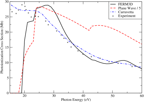
Figure 3: (Color online) $N_{2}$ photoionization cross sections vs photon energy. Calculations made using FERM3D and the plane wave approximation are compared to experimental measurements taken from [13].

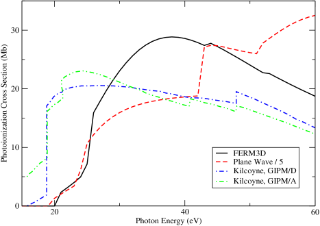
Figure 4: (Color online) $F_{2}$ photoionization cross sections vs photon energy. Calculations made using FERM3D and the plane wave approximation are compared to theoretical calculations taken from [14].

The principles seen in the case of the 1D square well also limit tomographic reconstruction in true molecular systems, although molecular systems are much more computationally challenging due to the complicated potentials which describe the electron-ion interaction. We calculate the electron-ion scattering states using FERM3D [12], a code which is designed for the highly non-centrosymmetric potentials seen in these systems. This potential is described by $V_{mol}=V_{s}+V_{ex}+V_{pol}$, where $V_{s}$ is the local electrostatic potential, $V_{ex}$ is the exchange potential arising from antisymmetrization of the wavefunction and treated in the local density approximation, and $V_{pol}$ is a polarization potential that describes the relaxation of the target under the influence of the incoming electron. Figure 3 compares the total photoionization cross section for $N_{2}$ calculated with FERM3D and the plane wave approximation to a prior calculation and experiment [13], while Figure 4 compares cross sections for $F_{2}$ to a previous calculation[14]. For both molecules, FERM3D gives cross sections with sizes comparable to prior calculations, with photoionization maxima shifted higher than in the comparison. In both molecules, the plane wave cross sections are too large by a factor of five.

The calculated dipole matrix elements may also be used to tomographically reconstruct the molecular orbitals. In a tomography experiment, the experimentally measurable quantity is the dipole matrix element between a bound state of the molecule and a scattering state whose incoming-wave portion asymptotically goes to $e^{i\vec{k}\cdot\vec{x}}$.

For incoming-wave boundary conditions, FERM3d calculates dipole matrix elements

$$d^{q}_{E;l,m}=\mathinner{\langle{\psi^{(-)}_{E;l,m}}|}\hat{\epsilon}_{q}\cdot\vec{x}\mathinner{|{\psi_{g}}\rangle}$$ (20)

where $\psi^{(-)}_{E;l,m}$ is an energy-normalized wavefunction which obeys incoming-wave boundary conditions [15]

$$\begin{split}\lim_{r\to\infty}\psi^{(-)}_{E;l,m}=\sum_{l^{\prime},m^{\prime}}Y_{lm}(\hat{r})(2i)^{-1}(f_{l}^{+}(r)\delta_{l,l^{\prime}}\delta_{m,m^{\prime}}-\\ f_{l}^{-}(r)S^{{\dagger}}_{l,m;l^{\prime},m^{\prime}}).\end{split}$$ (21)

where

$$f^{\pm}_{l}(r)\to_{r\to\infty}e^{\pm i(kr-l\pi/2+\sigma_{l}+1/k\ln{2kr})}$$ (22)

are radially outgoing/incoming Coulomb spherical waves, as defined in [16] and $\sigma_{l}=\text{arg}(\Gamma(l+1-i/k))$ is the Coulomb phase shift.

To find $d^{q}_{\vec{k}}$, it is now necessary to find the superposition $\psi_{\vec{k}}=A_{lm}(\vec{k})\psi_{E;lm}$ whose outgoing component matches the outgoing component of $e^{i\vec{k}\cdot\vec{x}}$. Expanding

$$e^{i\vec{k}\cdot\vec{x}}=4\pi\sum_{l,m}i^{l}j_{l}(kr)Y_{l,m}(\hat{x})Y^{*}_{lm}(\hat{k})$$ (23)

where $j_{l}(kr)\to_{r\to\infty}(2i)^{-1}(e^{i(kr-l\pi/2)}-e^{-i(kr-l\pi/2)})$ are spherical Bessel functions, matching coefficients of $Y_{lm}(r)e^{ikr}$ yields

$$A_{lm}(\vec{k})=4\pi i^{l}e^{-i\sigma_{l}}Y^{*}_{lm}(\hat{k})k^{1/2}$$ (24)

where the factor of $k^{1/2}$ converts the energy-normalized matrix elements calculated in FERM3D to momentum normalization.

$\vec{d}_{\vec{k}}$ is now given by

$$\vec{d}^{q}_{\vec{k}}=\sum_{l,m}\vec{d}^{q}_{l,m}(k^{2}/2)A_{l,m}(\vec{k})$$ (25)

As in the 1D square well, the tomographic image of the orbital may now be computed by substituting the calculated $\vec{d}_{\vec{k}}$ for the experimentally measured quantity in the tomographic reconstruction procedure. As photoionization is not limited to the molecular HOMO, tomographic images may be calculated for all the orbitals of a molecule. Such tomographic images will in general be complex-valued, and will differ according to which polarization component is used for the tomographic procedure.

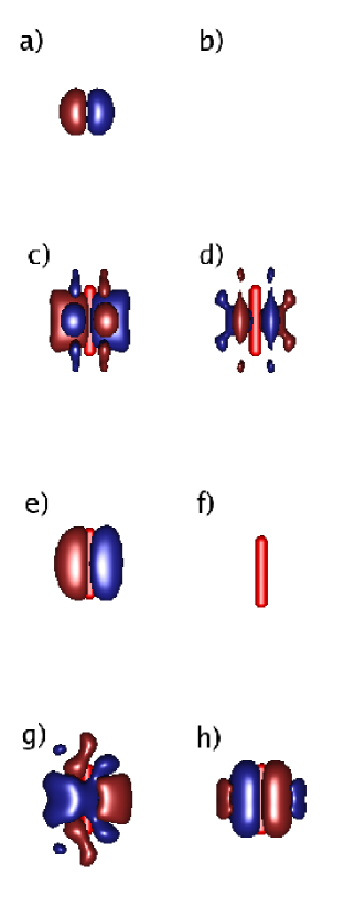
Figure 5: (Color online) Comparison of the Hartree-Fock orbital and associated tomographic images for the $N_{2}$ $1\Pi_{u}$ orbital. a) and b) give the real and (zero) imaginary components of the Hartree-Fock orbital. c) and d) give the real and imaginary components of the tomographic image made from the x-polarized dipole matrix element. e) and f) give the real and imaginary components of the tomographic image made from the y-polarized dipole matrix element. g) and h) give the real and imaginary components of the tomographic image made from the z-polarized dipole matrix element.

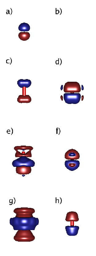
Figure 7: (Color online) Comparison of the Hartree-Fock orbital and associated tomographic images for the $N_{2}$ $2\Sigma_{u}$ orbital. a) and b) give the real and (zero) imaginary components of the Hartree-Fock orbital. c) and d) give the real and imaginary components of the tomographic image made from the x-polarized dipole matrix element. e) and f) give the real and imaginary components of the tomographic image made from the y-polarized dipole matrix element. g) and h) give the real and imaginary components of the tomographic image made from the z-polarized dipole matrix element.

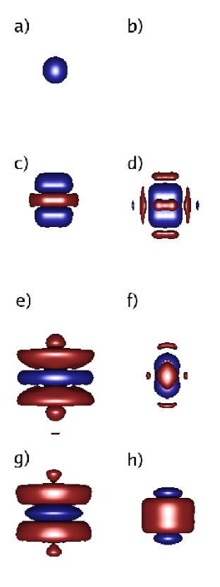
Figure 8: (Color online) Comparison of the Hartree-Fock orbital and associated tomographic images for the $N_{2}$ $2\Sigma_{g}$ orbital. a) and b) give the real and (zero) imaginary components of the Hartree-Fock orbital. c) and d) give the real and imaginary components of the tomographic image made from the x-polarized dipole matrix element. e) and f) give the real and imaginary components of the tomographic image made from the y-polarized dipole matrix element. g) and h) give the real and imaginary components of the tomographic image made from the z-polarized dipole matrix element.

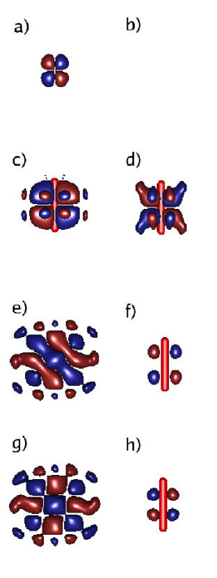
Figure 9: (Color online) Comparison of the Hartree-Fock orbital and associated tomographic images for the $F_{2}$ $1\Pi_{g}$ orbital. a) and b) give the real and (zero) imaginary components of the Hartree-Fock orbital. c) and d) give the real and imaginary components of the tomographic image made from the x-polarized dipole matrix element. e) and f) give the real and imaginary components of the tomographic image made from the y-polarized dipole matrix element. g) and h) give the real and imaginary components of the tomographic image made from the z-polarized dipole matrix element.

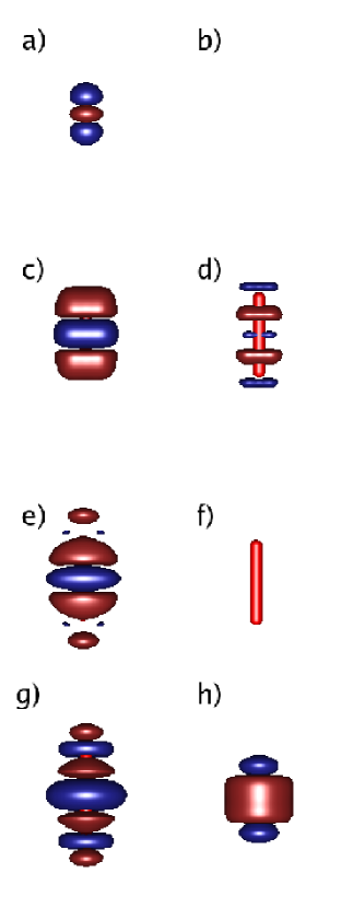
Figure 10: (Color online) Comparison of the Hartree-Fock orbital and associated tomographic images for the $F_{2}$ $3\Sigma_{g}$ orbital. a) and b) give the real and (zero) imaginary components of the Hartree-Fock orbital. c) and d) give the real and imaginary components of the tomographic image made from the x-polarized dipole matrix element. e) and f) give the real and imaginary components of the tomographic image made from the y-polarized dipole matrix element. g) and h) give the real and imaginary components of the tomographic image made from the z-polarized dipole matrix element.

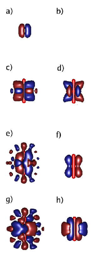
Figure 11: (Color online) Comparison of the Hartree-Fock orbital and associated tomographic images for the $F_{2}$ $1\Pi_{u}$ orbital. a) and b) give the real and (zero) imaginary components of the Hartree-Fock orbital. c) and d) give the real and imaginary components of the tomographic image made from the x-polarized dipole matrix element. e) and f) give the real and imaginary components of the tomographic image made from the y-polarized dipole matrix element. g) and h) give the real and imaginary components of the tomographic image made from the z-polarized dipole matrix element.

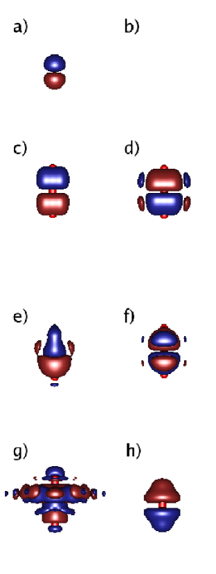
Figure 12: (Color online) Comparison of the Hartree-Fock orbital and associated tomographic images for the $F_{2}$ $2\Sigma_{u}$ orbital. a) and b) give the real and (zero) imaginary components of the Hartree-Fock orbital. c) and d) give the real and imaginary components of the tomographic image made from the x-polarized dipole matrix element. e) and f) give the real and imaginary components of the tomographic image made from the y-polarized dipole matrix element. g) and h) give the real and imaginary components of the tomographic image made from the z-polarized dipole matrix element.

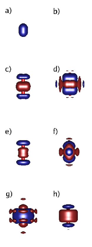
Figure 13: (Color online) Comparison of the Hartree-Fock orbital and associated tomographic images for the $F_{2}$ $2\Sigma_{g}$ orbital. a) and b) give the real and (zero) imaginary components of the Hartree-Fock orbital. c) and d) give the real and imaginary components of the tomographic image made from the x-polarized dipole matrix element. e) and f) give the real and imaginary components of the tomographic image made from the y-polarized dipole matrix element. g) and h) give the real and imaginary components of the tomographic image made from the z-polarized dipole matrix element.

We present tomographic images of various orbitals of $N_{2}$ and $F_{2}$, calculated in the body-fixed frame using the x,y, and z polarization components. Each image is given with the real and imaginary components, and includes an orange bar (not always visible) extending between the two atoms of the molecule for the purposes of scale. For $N_{2}$, tomographic reconstructions for the $1\Pi_{u}$ (Fig. 5), $3\Sigma_{g}$ (Fig. 6), $2\Sigma_{u}$ (Fig. 7) and $2\Sigma_{g}$ (Fig. 8) orbitals are shown. For $F_{2}$, reconstructions were calculated for the $1\Pi_{g}$ (Fig. 9), $3\Sigma_{g}$ (Fig. 10), $1\Pi_{u}$ (Fig. 11), $2\Sigma_{u}$ (Fig. 12), and $2\Sigma_{g}$ (Fig. 13) orbitals.

For these example molecules, tomographic reconstruction tends to preserve the $\Sigma$ or $\Pi$, gerade or ungerade character of the orbitals in question. However, the reconstructed orbitals may display additional radial nodes not found in the original orbitals. Features which correspond to features of the original orbitals may be distorted in shape and size, and display a spatially varying complex phase. Finally, tomographic images of the same orbital made using different polarization information may produce differing images of the same orbital. Many of these features are also seen in [10], which treats the scattering process from a multielectron perspective, but does not consider the distorting effects of a molecular potential.

2 Conclusions

The use of rescattering electrons as a probe of molecular properties offers many exciting avenues for future research. However, the rescattering process is itself more complicated than has been recognized in early reconstruction efforts, and is worthy of study in its own right.

For molecular tomography, the results presented in this paper suggest that at energy scales where such distortion is significant, tomographic reconstructions may be significantly distorted from the “true” orbitals these methods seek to find. Nevertheless, for the example molecules presented here, the tomographic reconstruction procedure was able to successfully reproduce the $\Sigma$ or $\Pi$, gerade or ungerade nature of the orbitals in question. Reconstructions made using differently polarized dipole matrix elements gave different tomographic images of the same orbital, while reconstructions made from a particular polarization gave tomographic images with spatially varying complex phase. Both of these properties could be useful as an experimental check of reconstructed wavefunctions: ideal reconstructions would have a spatially uniform complex phase and reconstructions made with different polarization information should agree with one another. Additionally, experiments could use higher scattering energies to minimize the scattering state distortions due to interactions with the molecular potential.

The sensitivity of the scattering states to the molecular potential also offers the prospect for new types of experiments. Such experiments could monitor the movement of charge within the parent ion at ultrafast timescales. For example, a two-center interference experiment of the type discussed in [3] might observe the movement of charge in a diatomic molecule by observing interference maxima/minima occurring at different energies for the short and long rescattering trajectories.

We thank Nick Wagner for insightful and stimulating discussions. This work was supported in part by the Department of Energy, Office of Science, and in part by the NSF EUV ERC.

3 Appendix: Gauges and Dispersion Relations

Within the overall framework of the plane wave approximation, several heuristic methods have been suggested to improve the accuracy of tomographic reconstructions[3]. For the 1D square well, we considered the effects of phenomenological “dispersion relations” and reconstructions made in the momentum, rather than velocity gauge.

A dispersion relation attempts to correct for an electron’s shorter wavelength by substituting $e^{i\vec{q}\cdot\vec{x}}$ for $e^{i\vec{k}\cdot\vec{x}}$ in Equation 2, where $|\vec{q}|=\sqrt{2(k^{2}/2-\epsilon V)}$, where $V$ is the potential felt by the electron in the interaction region, and $\epsilon\in[0,1]$.

Tomography may also be performed in gauges other than the length gauge given in equation 2. If both continuum and bound wavefunctions are eigenstates of the Hamiltonian, the dipole matrix element is identical in the length

$$d^{(l)}_{k}=\mathinner{\langle{\psi_{g}}|}x\mathinner{|{\psi_{k}}\rangle}$$ (26)

and momentum

$$d^{(p)}_{k}=\frac{\mathinner{\langle{\psi_{g}}|}ip\mathinner{|{\psi_{k}}\rangle}}{E_{g}-E_{k}}$$ (27)

gauges. From the momentum gauge form of the dipole matrix element, and employing the plane wave approximation for $\mathinner{|{\psi_{k}}\rangle}$, it is possible to generate a second tomographic reconstruction

$$\psi^{(p)}(x)=\int dqe^{iq(k)x}d^{(p)}_{k}\frac{E_{g}-k^{2}/2}{-q(k)}.$$ (28)

As a plane wave is not an eigenfunction of the scattering Hamiltonian, this reconstruction will in general give a different image of the target orbital than a reconstruction made using the length gauge.

We tested both the length- and momentum-gauge tomographic reconstructions using dispersion relations $q(\epsilon)=\sqrt{2(k^{2}/2-\epsilon V)}$, using the overlap of the true wavefunction and its (normalized) tomographic image as a figure of merit. The test employed the same $V=-1.61$, $x_{0}=2.5$ potential and $E=-.5$ target wavefunction used to generate Figure 1.

Figure 2a gives the magnitude of the overlap between the two tomographic images and the ground state and between each other as a function of the dispersion parameter $\epsilon$. For this choice of potential and target orbital, the tomographic reconstructions gave a very poor overlap with the target orbital for $\epsilon\in[0,1]$, reaching a maximum magnitude of $0.60$ at $\epsilon=0.26$ in the momentum gauge. In the dipole gauge, the maximum overlap was achieved at $\epsilon=1.0$, also giving an overlap of magnitude 0.60. Figure 2b compares the maximally overlapping reconstructions to the true ground state wavefunction.

A perfect reconstruction would give the same image regardless of the gauge the tomographic procedure was performed in. However, agreement between images made in separate gauges does not guarantee the accuracy of the reconstruction. Although both gauges gave nearly identical tomographic images at $\epsilon=0$, the resulting images gave among the worst overlaps with the target orbital.

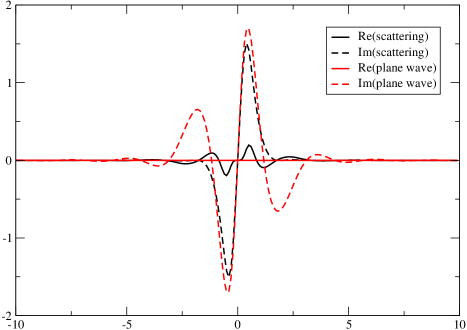
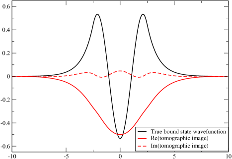
Figure 1: (Color online) The tomographic reconstruction procedure applied to the 1D square well. (Top) Comparison of dipole matrix elements $d_{k}=\mathinner{\langle{\psi_{c}(x)}|}x\mathinner{|{\psi_{g}(x)}\rangle}$, calculated using plane waves and scattering states for $\psi_{c}(x)$. (Bottom) Because the scattering state matrix elements differ from those calculated using plane waves, the reconstructed image of the orbital will differ from the true bound state wavefunction.

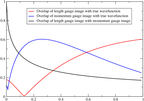
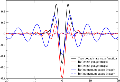
Figure 2: (Color online) a) Magnitude of the overlap between (normalized) tomographic images of a bound wavefunction and the true wavefunction, and between different tomographic images, calculated using $q(\epsilon)=\sqrt{2(k^{2}/2-\epsilon V)}$, $\epsilon\in[0,1]$. b) Comparison of the maximally overlapping tomographic images to the true wavefunction. In the momentum gauge, maximal overlap was obtained for $\epsilon=.26$, while in the length gauge, maximal overlap was obtained for $\epsilon=1$. Both images have been normalized and rotated to give a purely real overlap with the true wavefunction.

Figure 6: (Color online) Comparison of the Hartree-Fock orbital and associated tomographic images for the $N_{2}$ $3\Sigma_{g}$ orbital. a) and b) give the real and (zero) imaginary components of the Hartree-Fock orbital. c) and d) give the real and imaginary components of the tomographic image made from the x-polarized dipole matrix element. e) and f) give the real and imaginary components of the tomographic image made from the y-polarized dipole matrix element. g) and h) give the real and imaginary components of the tomographic image made from the z-polarized dipole matrix element.

References

- 1. Corkum, P. B. Phys. Rev. Lett. 1993, 71, 1994.
- 2. Lewenstein, M.; Balcou, P.; Ivanov, M. Y.; A.L’Huillier,; Corkum, P. B. Phys. Rev. A 1994, 49, 2117.
- 3. Lein, M. J. Phys. B 2007, 40, R135.
- 4. Plenge, J.; Nicolas, C.; Caster, A. G.; Ahmed, M.; Leone, S. R. J. Chem. Phys. 2006, 125, 133315.
- 5. Nugent-Glandorf, L.; Scheer, M.; Samuels, D. A.; Bierbaum, V. M.; Leone, S. R. J. Chem. Phys. 2002, 117, 6108.
- 6. Itatani, J.; Levesque, J.; Zeidler, D.; Niikura, H.; Pepin, H.; Kieffer, J. C.; Corkum, P. B.; Villeneuve, D. M. Nature 2004, 432, 867.
- 7. Walters, Z.; Tonzani, S.; Greene, C. H. J. Phys. B. 2007, 40, F277.
- 8. Morishita, T.; Le, A. T.; Chen, Z.; Lin, C. D. preprint .
- 9. Santra, R.; Gordon, A. Phys. Rev. Lett. 2006, 96, 073906.
- 10. Patchkovskii, S.; Zhao, Z.; Brabec, T.; Villeneuve, D. M. J. Chem. Phys. 2007, 126, 114306.
- 11. Smirnova, O.; Spanner, M.; Ivanov, M. J. Phys. B 2006, 39, S307.
- 12. Tonzani, S. Comp. Phys. Comm. 2007, 176, 146.
- 13. Carravetta, V.; Luo, Y.; Agren, H. Chem. Phys. 1993, 174, 141.
- 14. Kilcoyne, D. A. L.; Nordholm, S.; Hush, N. S. Chemical Physics 1986, 107, 197.
- 15. Breit, G.; Bethe, H. A. Phys. Rev. 1954, 93, 888.
- 16. Aymar, M.; Greene, C. H.; Luc-Koenig, E. Rev. Mod. Phys. 1996, 68, 1015.