Star cluster versus field star formation in the nucleus of the prototype starburst galaxy M82

We analyse high-resolution Hubble Space Telescope/Advanced Camera for Surveys imaging of the nuclear starburst region of M82, obtained as part of the Hubble Heritage mosaic made of this galaxy, in four filters (Johnson-Cousins equivalent $B,V$, and $I$ broad bands, and an H$\alpha$ narrow-band filter), as well as subsequently acquired $U$-band images. We find a complex system of $\sim$150 star clusters in the inner few 100 pc of the galaxy. We do not find any conclusive evidence of a cluster-formation epoch associated with the most recent starburst event, believed to have occurred about 4–6 Myr ago. This apparent evidence of decoupling between cluster and field-star formation is consistent with the view that star cluster formation requires special conditions. However, we strongly caution, and provide compelling evidence, that the ‘standard’ simple stellar population analysis method we have used significantly underestimates the true uncertainties in the derived ages due to stochasticity in the stellar initial mass function and the corresponding sampling effects.

1 Introduction

Supermassive star clusters or ‘super star clusters’ (SSCs) are highly luminous and massive, yet compact star clusters. They result from the most intense star-forming episodes that are believed to occur at least once in the lifetime of nearby starburst galaxies, and most probably also in merging galaxies at high redshift (Smith et al. 2006). Super star clusters have been observed using the Hubble Space Telescope (HST) in interacting, amorphous, dwarf, and starburst galaxies, (e.g., Arp & Sandage 1985; Melnick, Moles & Terlevich 1985; Holtzman et al. 1992; Meurer et al. 1992; Whitmore et al. 1993, 1999; Hunter et al. 1994, 2000; O’Connell, Gallagher & Hunter 1994; Ho & Filippenko 1996; Conti, Leitherer & Vacca 1996; Watson et al 1996; Ho 1997; Carlson et al. 1998; de Grijs, O’Connell & Gallagher 2001; de Grijs et al. 2003a,b; and references therein) and are thought to be contemporary analogues of young globular clusters. For this reason, the study of SSCs can lead to an understanding of the formation, evolution, and destruction of globular clusters (see the review by de Grijs & Parmentier 2007) as well as of the processes of star formation in extreme environments.

A current issue of strong contention relates to the stellar initial mass function (IMF) in starburst environments, and particularly whether it is ‘abnormal’ due to preferential production of higher-mass stars (we will touch on this issue below, where we explore the effects of stochasticity in the IMF). Furthermore, SSCs are involved in the activation and feeding of supergalactic winds (e.g., Tenorio-Tagle, Silich & Muñoz-Tuñón 2003; Westmoquette et al. 2007a,b). In addition, SSCs can be age-dated individually using either spectroscopic or multi-passband imaging observations, and as such they can be used as powerful tracers of the starburst history across a given galaxy.

The target galaxy discussed in this paper, M82, is the prototype nearby starburst galaxy. The starburst is five times as luminous as the entire Milky Way, and it has one hundred times the luminosity of the centre of our Galaxy (O’Connell et al. 1995; and references therein). At a distance of 3.9 Mpc (Sakai & Madore 1999), many of M82’s individual clusters can easily be resolved by the HST. O’Connell et al. (1995) performed an optical imaging study of the central region of M82 using the HST’s Wide Field / Planetary Camera (WF/PC), and unveiled over one hundred candidate SSCs (in their nomenclature) within the visible starburst region, with a mean $M_{V}\sim-11.6$ mag (based on an adopted distance of 3.6 Mpc). At the present time, this is brighter than any globular cluster in the Local Group (e.g., Ma et al. 2006; and references therein). A more recent study by Melo et al. (2005) used HST/Wide Field and Planetary Camera-2 (WFPC2) observations to reveal 197 young massive clusters in the starburst core (with a mean mass close to $2\times 10^{5}$ M_⊙, largely independent on the method used to derive these masses), confirming this region as a most energetic and high-density environment (see also Mayya et al. 2008).

Unfortunately, studies of the core are inhibited by M82’s almost edge-on inclination ($i\sim 80^{\circ}$; Lynds & Sandage 1963; McKeith et al. 1995) and the great deal of dust within the galactic disk (see Mayya et al. 2008 and references therein). Although the dust provides the raw material for the clusters’ formation, it also obscures and reradiates most of the light from the starburst in the infrared (Keto et al. 2005). However, despite all the bright sources associated with the active starburst core suffering from such heavy extinction (in the range $A_{V}\sim 5$–25 mag; e.g., Telesco et al. 1991; McLeod et al. 1993; Satyapal et al. 1995; Mayya et al. 2008, and references therin), many individual clusters remain bright enough to obtain good photometry and spectroscopy for (see, for example, Smith et al. 2006; McCrady & Graham 2007).

The starburst galaxy M82 has recently experienced at least one tidal encounter with its large spiral neighbour galaxy, M81, resulting in a large amount of gas being channelled into the core of the galaxy over the last 200 Myr (e.g., Yun, Ho & Lo 1994). The most major recent encounter is believed to have taken place roughly $(2-5)\times 10^{8}$ yr ago (Brouillet et al. 1991; Yun et al. 1994; see also Smith et al. 2007), causing a concentrated starburst and an associated pronounced peak in the cluster age distribution (e.g., de Grijs et al. 2001, 2003c; Smith et al. 2007). This starburst continued for up to $\sim 50$ Myr at a rate of $\sim 10$ M_⊙ yr^-1 (de Grijs et al. 2001). Two subsequent starbursts ensued, the most recent of which (roughly 4–6 Myr ago; Förster Schreiber et al. 2003, hereafter FS03; see also Rieke et al. 1993) may have formed at least some of the core clusters (Smith et al. 2006) – both SSCs and their less massive counterparts (see Section 3.6).

The active starburst region in the core of M82 has a diameter of 500 pc and is defined optically by the high surface brightness regions, or ‘clumps’, denoted A, C, D, and E by O’Connell & Mangano (1978). These regions correspond to known sources at X-ray, infrared, and radio wavelengths, and as such they are believed to be the least obscured starburst clusters along the line of sight (O’Connell et al. 1995). The galaxy’s signature bi-polar outflow or ‘superwind’ appears to be concentrated on regions A and C (Shopbell & Bland-Hawthorn 1998; Smith et al. 2006; Silich et al. 2007), and is driven by the energy deposited by supernovae, at a rate of $\sim 0.1$ supernova yr^-1 (e.g., Lynds & Sandage 1963; Rieke et al. 1980; Fabbiano & Trinchieri 1984; Watson, Stranger & Griffiths 1984; McCarthy, van Breugel & Heckman 1987; Strickland, Ponman & Stevens 1997; Shopbell & Bland-Hawthorn 1998; see also de Grijs et al. 2000 for a review)

This paper is organised as follows. In Section 2 we give an overview of the observations, source selection, and image processing techniques applied to our sample of star clusters in the core of M82. Section 3 describes the methods and results of the age determinations, and the complications due to stochasticity in the IMF, and Section 4 provides a summary and discussion of these results, where we place our star cluster results in the context of the star-formation history of the galaxy.

2 Source Selection and Photometry

2.1 Observations

During March 2006, a large four-filter six-point mosaic data set of M82 was obtained as part of the Hubble Heritage Project (HST proposal GO-10776) using the Advanced Camera for Surveys/Wide Field Channel (ACS/WFC; pixel size $\sim 0.05$ arcsec). Exposure times were 1600, 1360, 1360, and 3320 s for observations in the F435W (equivalent to Johnson $B$), F555W ($\sim V$), F814W ($\sim I$), and F658N (H$\alpha$) filters, respectively. For each of these filters, four exposures were taken at six marginally overlapping pointings, or ‘tiles’. The four exposures within each tile were dithered to improve the rejection of detector artefacts and cosmic rays, and to span the interchip gap of the ACS/WFC. The final mosaic of the $3\times 2$ ACS/WFC fields was pipeline-processed by the HST data archive’s standard reduction routines; for full details of the observing programme, image processing and calibration, see Mutchler et al. (2007).

Whereas O’Connell et al. (1995) had access to two broad-band filters only (F555W and F785LP, the latter corresponding to a broad $\sim R$-band filter), the present study uses these four-filter high-resolution ACS Hubble Heritage observations of M82 as well as subsequently acquired F330W ($\sim U$-band) data, observed as part of proposal GO-10609 (PI Vacca), and obtained from the HST data archive. The F330W observations centred on M82 A and C were obtained on UT December 7 and 8, 2006, respectively, with the ACS/High Resolution Camera (ACS/HRC; pixel size $\sim 0.028\times 0.025$ arcsec). The respective exposure times were 4738 and 3896 s, with the ACS/HRC pointed under a position angle of 90.08 and 90.06^∘ (East with respect to North), respectively. The two final pipeline-processed and flux-calibrated images cover adjacent fields, largely coincident with the central starburst area selected for further study in the current paper (see Section 2.2).

It should also be noted that O’Connell et al. (1995) used pre-COSTAR data, acquired before the first HST servicing mission. The increased volume and quality of data now available to us provides more evidence with which to distinguish clusters from point sources (i.e., stars), and in principle allows for better constrained age estimates, making the data set ideally matched for the first comprehensive comparison of the various star-formation modes in one of the most violent environments in the local Universe.

2.2 Basic Image Processing

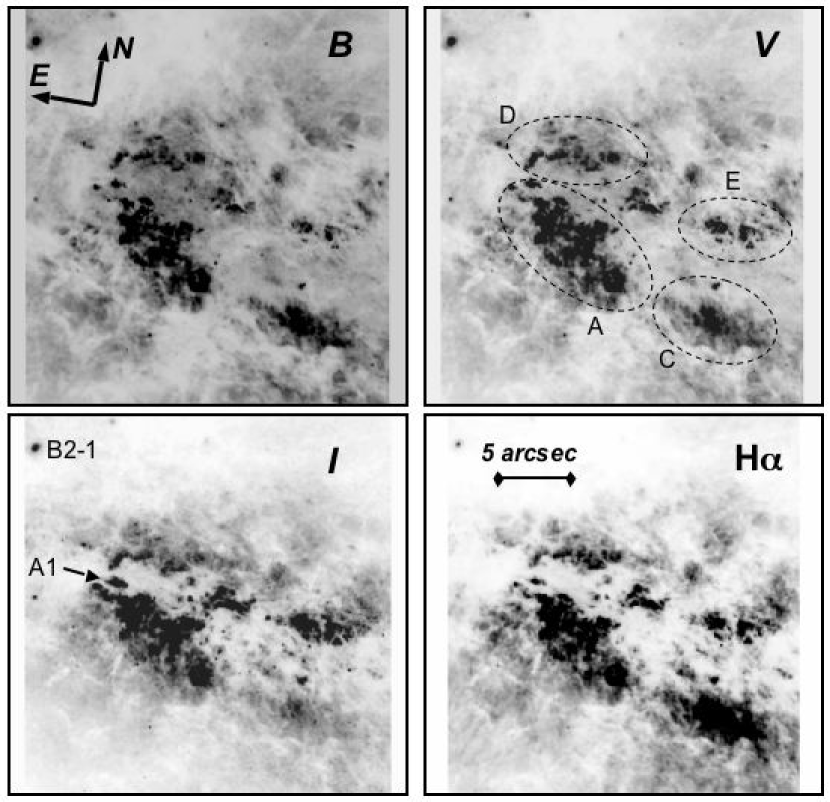
Figure 1: The starburst core region of M82 used for the main analysis in this paper. The four panels show the region’s appearance as a function of wavelength ($B$: F435W; $V$: F555W; $I$: F814W; H$\alpha$: F658N). Each panel is 29.55 arcsec on a side; a scale bar of 5 arcsec length (corresponding to $\sim 95$ pc at the distance of M82) is shown in the bottom right-hand panel. In the top right-hand panel, we show the outlines of regions A, C, D, and E, defined by O’Connell & Mangano (1978), superposed on the $V$-band image. The bottom left-hand panel includes the positions of clusters A1 and B2-1 (see Smith et al. 2006). The individual panels are displayed at optimum dynamic range, in order to emphasise the low-level structure.

The final drizzled $B,V,I$, and H$\alpha$ images were first aligned using the iraf/stsdas tasks imalign and rotate, using a selection of conspicuous sources common to each frame as guides. They were then cropped to a common size of $541\times 591$ pixels ($27.05\times 29.55$ arcsec) in order to include only the very core of the galaxy, the region of particular interest in this paper. The $U$-band images were rotated, aligned and scaled to the Hubble Heritage data set using a similar selection of point-like sources common to both data sets, where available. This ensured that the astrometric solutions of all images were calibrated to a common frame of reference.

The selected region was chosen to specifically encompass the areas A, C, D, and E (O’Connell & Mangano 1978), as well as cluster B2-1 (de Grijs et al. 2001; Smith et al. 2006) for reasons of both image alignment and for photometric consistency checks. The starburst region studied in detail in this paper is shown in Fig. 1. In Fig. 2 we show the complementary, mosaicked F330W ACS/HRC observations, rotated to the same orientation as the fields in Fig. 1.

At first glance, the images in the individual passbands exhibit a number of striking similarities as well as differences. It is clear that the M82 core is undergoing vigorous star formation, as indicated by the strong H$\alpha$ and F330W-band emission. A first impression of the various named regions indicates that region C may be the youngest (since it does not exhibit strong emission in the $I$-band filter), while region E might be somewhat older or most affected by extinction (given that it is progressively easier to identify as a function of increasing wavelength). We will quantify these first impressions in Section 3.

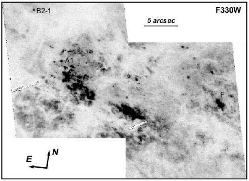
Figure 2: Complementary F330W observations of the M82 A (east) and M82 C (west) pointings obtained with the ACS/HRC. The position angle is identical to that of the four images shown in Fig. 1; clusters A1, B2-1, and F (e.g., Gallagher & Smith 1999) are indicated for orientation. The mosaic is displayed at optimum dynamic range, in order to emphasise the low-level structure. The linear features on the left-hand side of each of the two mosaicked pointings, seen under an angle of about 30^∘, are instrumental artefacts due to the HRC’s coronographic finger. The occulting finger is not retractable and is therefore present in every ACS/HRC exposure.

2.3 Source Selection

The standard deviations of the number of counts of seemingly empty sections of all images were established to ascertain a ‘sky’ background count for each filter. Multiples of this background count were then used as thresholds above which the number of sources in each filter was calculated, using the idl find task. Figure 3 shows that the most suitable, conservatively chosen thresholds for source inclusion were 0.08, 0.20, and 0.90 counts s^-1, for the $B,V$, and $I$ bands, respectively. (In view of the more stringent requirements applied in the next steps in the construction of our final sample, the exact values of these thresholds are unimportant, as long as they are chosen such that no real objects are omitted a priori at this stage.) For all three passbands, initially the number of detections decreases rapidly with increasing threshold value. This is an indication that our ‘source’ detections are noise dominated. Where the rapid decline slows down to a more moderate rate, our detections become dominated by ‘real’ objects (either stars, clusters, or real intensity variations in the background field). In Fig. 3 we have indicated the approximate count rates of these transitions by the vertical dashed lines; in the remainder of this paper we will only consider the objects in the ‘source-dominated’ domain, as indicated in the three panels.

We point out that the curve delineated by the data points is not as smooth as perhaps expected at face value. This is due to our use of a number of different ranges of relatively low background flux in which we determined the standard deviations of the counts. We subsequently ran our find routine based on detection thresholds in multiples of the various standard deviations. The deviations from continuous smooth curves are therefore a good indication of the intrinsic variations in seemingly empty field regions at low flux levels.

Figure 3: Number of objects detected as a function of threshold level for the $B,V$, and $I$ images. The vertical dashed lines show the thresholds adopted here for source-dominated (as opposed to noise-dominated) ranges. See the text for details (Section 2.3).

We subsequently employed a cross-identification procedure to determine how many sources were visible and coincident with intensity peaks within 1.4 pixels of each other in all three filters (i.e., allowing for 1-pixel mismatches in both spatial directions), yielding over 900 potential clusters. Sources found to be present in all filters were then confirmed individually by eye, owing to the lack of a more robust verification procedure in the presence of the highly variable background and significantly variable extinction across our field of view (cf. de Grijs et al. 2001; Smith et al. 2007). This verification process was performed independently by two of us, and the small number of disagreements (less than a few tens of objects) were discussed and revisited in detail in order to construct the most robust and impartial cluster sample possible.

In our next step we used the ‘Tiny Tim’ software package (Krist & Hook 1997) to generate HST point-spread functions (PSFs). We determined the best-fitting Gaussian profile for each candidate cluster, as well as for the Tiny Tim PSFs. The width of the latter was found to be best represented by a Gaussian profile of $\sigma_{\rm G}=1.38$ pixels, in the $V$ band. Any candidate cluster with $\sigma_{\rm G}$ (significantly) below this value was considered most likely to be a star (or an artefact either of the CCD or due to cosmic rays) and was consequently discarded. Artificial clusters were then created using the BAOlab package (Larsen 1999), using HST/ACS PSFs, and their $\sigma_{\rm G}$ values were compared with those determined by our idl routine. This provided an additional constraint with which to distinguish clusters from stars, leaving 208 clusters for further analysis. We note that although realistic cluster luminosity profiles may well deviate from the simple Gaussian profile adopted here, its consistent and systematic application to our observations allows us to robustly differentiate between objects of different sizes, irrespective of their true profiles, provided that the profiles of the individual objects do not differ too much from object to object. In Fig. 4 we display the distribution of our final cluster sample across the face of the M82 starburst core in the $V$ band. This final sample was used for further analysis in all of the $U,B,V,I$, and H$\alpha$ images.

The right-hand panel of Fig. 4 shows the distribution of the H$\alpha$ excess across the region. To produce this panel, we constructed the interpolated H$\alpha$ continuum from a combination of the $V$ and $I$-band images, scaled by their filter widths and exposure times. The image shows the ratio of the H$\alpha$ image and its continuum. The darkest shading corresponds to the most significant H$\alpha$ excess; the lightest shading to no (or a negligible) excess. We will discuss this image in Section 3.6.

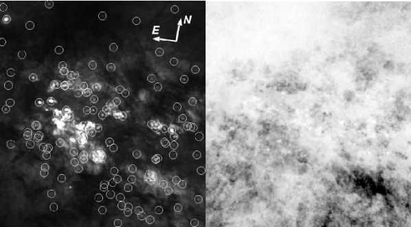
Figure 4: (left) Distribution of our final, cross-matched cluster sample across the face of the M82 starburst core, superposed on the $V$-band image. (right) H$\alpha$ excess distribution. The darkest shading corresponds to the most significant H$\alpha$ excess; the lightest shading indicates no (or an insignificant) excess. The orientation and scale of the images are as in Fig. 1.

2.4 Photometry

Two photometry tasks were used, in idl, with the aim of robustly determining the magnitudes of as many clusters as possible. The apphot task was used with source radii ranging from 1–10 pixels and a standard sky annulus with radii from 10 to 15 pixels, corresponding to a linear scale of 10 to 14 pc at the distance of M82. In addition, our custom-written task photom utilises radii individualised for each cluster (based on visual inspection). The resulting ‘instrumental’ magnitudes (in the $U,B,V$, and $I$ bands) of the 152 clusters for which our tasks could robustly obtain photometry were adjusted for their zero-point offsets (determined from the headers of the archival HST observations).

In Anders, Gieles, & de Grijs (2006) we carefully considered the implications and remedies of taking ‘sky’ annuli too close to a given cluster, in the sense that we would oversubtract the sky level because of the inclusion of flux from the cluster’s outer profile. We generated an extensive and systematic grid of aperture corrections as a function of filter, radius of the sky annulus, and cluster profile. Using these improved aperture corrections, we corrected our cluster aperture photometry based on a fixed source aperture for the systematic effects introduced by our reduction procedure. Upon close examination of our aperture choice, we concluded that a 3-pixel (radius) source aperture resulted in the smallest photometric scatter for the cluster sample as a whole. We will adopt this source aperture below. The resulting average (aperture-corrected) magnitudes of the clusters were 20.0, 19.5, and 19.3 mag in the $B,V$, and $I$ bands, respectively, with our cluster photometry spanning in excess of four magnitudes in all filters (5 mag in the $I$ band).

Although the data reduction procedure employed does not allow us to perform a proper assessment of the observational completeness limits, the luminosity functions in the $B,V$, and $I$ bands indicate that our detection limits are at $B\simeq 23.5,V\simeq 23$, and $I\simeq 24$ mag. As also shown in Fig. 3, where we showed the number of detected objects as a function of our detection threshold, our combined $BVI$ photometry is limited by the $B$ and $V$-band observations.

In Section 3 we will analyse our cluster photometry based on the cluster colours. In essence, we will use a poor man’s approach to cluster spectroscopy by using the broad-band spectral energy distributions (SEDs). Since a small change in colour could lead to a large change in the derived age, it is important to make sure that the application of the Anders et al. (2006) aperture corrections has not introduced unwanted systematic effects and/or offsets. Therefore, in Fig. 5 we compare the cluster colours derived from our variable-aperture photometry (obtained with the photom task) to those from the standard apertures (based on apphot) combined with the Anders et al. (2006) aperture corrections. Considering the representative uncertainties in the derived colours (shown in the bottom right-hand corners of both panels), both panels of Fig. 5 show excellent agreement between the two data sets. We are therefore confident that these aperture corrections will not introduce systematic offsets in the age determinations in Section 3.

Figure 5: Comparison of our $(B-V)$ and $(V-I)$ colours obtained from variable aperture photometry according to the actual cluster sizes, with fixed 3-pixel (radius) aperture photometry and aperture corrections from Anders et al. (2006). For reasons of clarity we have not added error bars to the data points; a representative set of error bars is shown in the bottom right-hand corner of each panel. The dotted lines of equality are shown to guide the eye.

3 Cluster ages

In this section we use the broad-band photometry derived in Section 2 to obtain estimates (or otherwise) of the star cluster ages in the M82 starburst core. For optimum results, we do not only require a sufficiently high age resolution in our models, but also take into account the effects on the integrated luminosities of statistically sampling the stellar IMF (e.g., Cerviño, Luridiana, & Castander 2000; Cerviño et al. 2002; Cerviño & Luridiana 2004, 2006). We will first discuss issues related to statistically sampling the IMF (Sections 3.1–3.4), and then apply the ‘standard’ analysis, essentially ignoring these issues, in Sections 3.5 and 3.6. This will highlight the differences caused by stochasticity in the IMF of incompletely sampled clusters.

3.1 Spectral synthesis models and isochrones

In order to achieve these aims, we have made use of the cmd2.0 tool, which provides the isochrones and the mean integrated magnitudes for a number of photometric systems, including HST/ACS data in the ST system used here. We calculated the integrated magnitudes for simple stellar populations (SSPs) based on a Kroupa (2001) IMF (corrected for binaries), covering a mass range from 0.15 to 120 M_⊙, from the solar metallicity ($Z=0.019$) isochrones of Girardi et al. (2002) and Marigo et al. (2008) for stars more massive than 7 M_⊙, and the Bertelli et al. (1994) isochrones for low-mass stars. Near-solar metallicity should be a reasonable match to the young objects in M82 (e.g., Gallagher & Smith 1999; see also Smith et al. 2006). Fritze-von Alvensleben & Gerhard (1994) also find, from chemical evolution models, that young clusters should have $Z\sim 0.3$–1.0 Z_⊙. Magnitudes and other quantities are based on Kurucz (1992) atmosphere models, except for cool stars (see Girardi et al. 2000 for more details).

Our set of SSP models and isochrones covers an age range from 1 Myr to 10 Gyr. We note, as a caveat, that the models do not include nebular emission, which may systematically affect the results at the youngest ages (see also Anders & Fritze-von Alvensleben 2003). We will return to this issue below (Section 3.7), where we discuss the results from the H$\alpha$ observations in detail.

Finally, we adopted the Galactic extinction law of Rieke & Lebofsky (1985; conveniently tabulated by Jansen et al. 1994) to correct our cluster photometry for foreground extinction in M82. Referring to fig. 1 of de Grijs et al. (2005), we note that the choice of extinction law in the optical wavelength range is relatively unimportant in the context of extinction corrections of broad-band photometry. Galactic foreground extinction was estimated based on Schlegel et al. (1998).

3.2 The ‘lowest-luminosity limit’ test

Estimates of physical parameters (such as mass or age) based on synthesis models assume a certain proportionality between the stars at different evolutionary phases for a given age. Of course, the use of the mean integrated luminosity provided by the SSP models only makes sense when this proportionality is robustly met. This implies that there must be sufficient numbers of stars in any and all evolutionary phases or, equivalently, that the IMF is well sampled in all relevant mass intervals (see Cerviño & Valls-Gabaud 2008 for a more detailed discussion).

The simplest test to identify whether the IMF is appropriately sampled is to use the ‘lowest-luminosity limit’ (LLL) method (Cerviño & Luridiana 2004). The LLL method states that the IMF is not sufficiently well sampled if the integrated luminosity of a cluster is lower than the luminosity of the most luminous star included in the model for the relevant age (see Pessev et al. 2008 for an application). This implies that clusters fainter than this limit cannot be analysed using standard procedures, including $\chi^{2}$ minimisation of the observed values with respect to the mean SSP models (but see Sections 3.5 and 3.6). Below the LLL, the proportionality assumed in the mean SSP value is not met, and the cluster colours do not reflect the cluster age of the entire population, but – instead – the colour combination of a given set of individual (luminous) stars. Consequently, in this case cluster ages and masses cannot be obtained self-consistently (although this caveat is largely ignored in most studies using SED fits to obtain cluster ages).

Figure 6 shows the LLL values as a function of age for the different filters used in this paper. These luminosities were obtained by identifying the most luminous star on each isochrone for the relevant passband. The dark-grey area corresponds to the ‘source-dominated’ clusters (cf. Fig. 3), assuming a distance $D=3.9$ Mpc to M82. The light-grey area shows the cluster’s maximum absolute luminosity, assuming an extinction of $A_{V}=4.0$ mag (roughly matching the mean extinction value of Melo et al. 2005; see also Mayya et al. 2008). The upper luminosity limit has been corrected for extinction using $A_{\mathrm{F435W}}=1.317A_{V},A_{\mathrm{F555W}}=0.98A_{V}$, and $A_{\mathrm{F814W}}=0.599A_{V}$, i.e., the corresponding corrections for a G2V-type star using a Cardelli et al. (1989) extinction law and a total-to-selective extinction ratio, $R_{V}=3.1$.

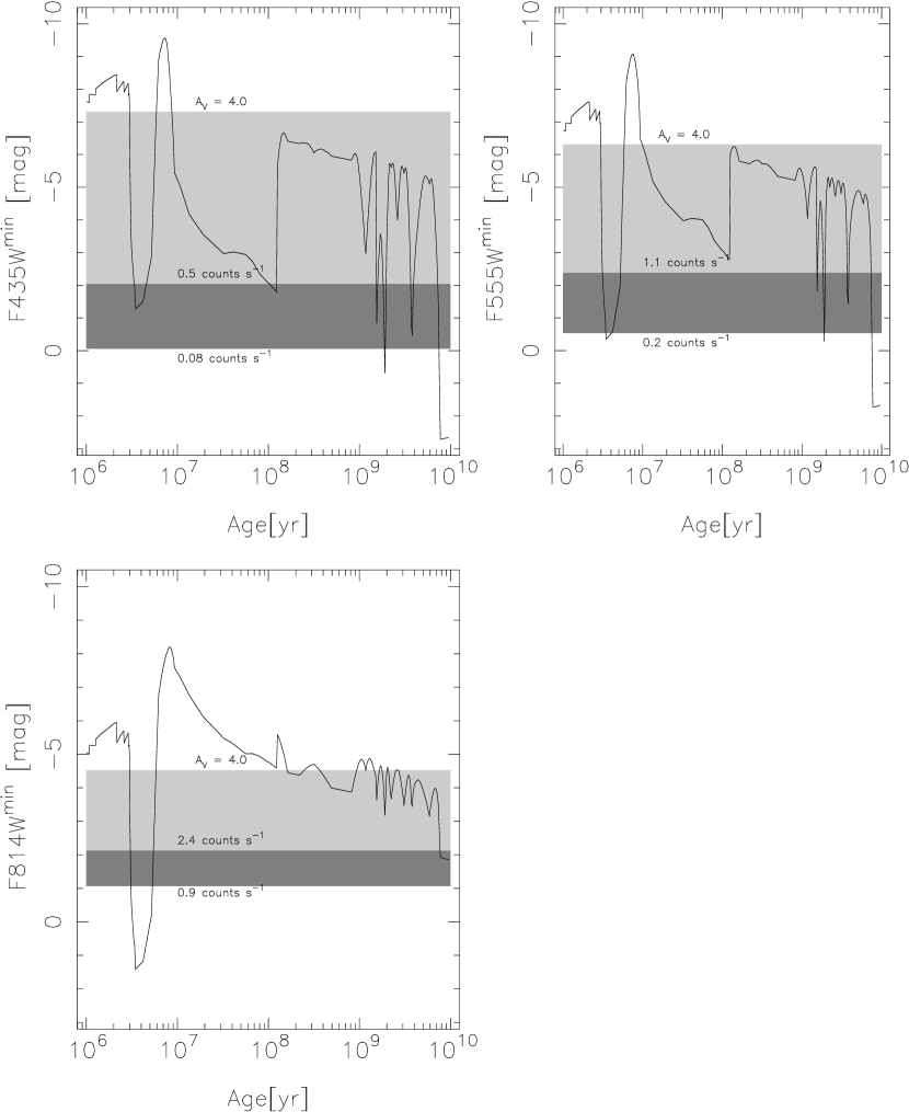
Figure 6: Lowest-luminosity limit for the ACS/WFC filters used here. The dark-grey area corresponds to the ‘source-dominated’ clusters (Fig. 3), assuming a distance to M82 of $D=3.9$ Mpc. The light-grey area shows the cluster’s maximum absolute magnitude assuming an extinction of $A_{V}=4.0$ mag. See the text for details.

We see that most of our clusters lie below the LLL, except in the age range around 2.5–6 Myr. When an extinction correction of $A_{V}=4$ mag is used, most clusters still lie below the LLL, particularly in the $I$ band. This means that, in general, none of our clusters can host the most luminous star that would be present theoretically for the given cluster age. This does not mean, however, that our sample clusters cannot host the occasional massive, evolved, red star (see for examples, e.g., Bruhweiler et al. 2003; Jamet et al. 2004; Pellerin 2006). However, in this case, gaps in the sampling of the cluster mass function are an a posteriori consequence of applying the LLL test.

3.3 Age estimates of incompletely sampled clusters

In the previous section we established that our clusters are affected by strong IMF sampling effects, so that age and mass estimates based on direct comparisons with SSP mean values are not valid (although we will show below what one would conclude in terms of cluster ages and the implications for the cluster-formation history in the centre of M82 if we were to ignore this caveat). As an example, red cluster colours could be explained as being caused by the absence of massive stars, but this absence can – in turn – be explained by either an old population in which the massive stars have faded, or a young population without massive stars (at least not to the extent expected theoretically), because of sampling effects (i.e., there are not enough stars to fully populate the massive-star tail of the IMF). In an analogous manner, cluster masses cannot be obtained properly, since the mass-luminosity relation depends on both the age and the cluster mass itself, and both are unknown quantities.

However, we can still obtain partial information about the clusters from their integrated luminosities, taking advantage of the sensitivity of different observables with respect to both stellar populations and individual stars. In doing so, one needs to take into account several basic rules, which we will now discuss.

3.3.1 General considerations and rules

First, the position of single stars in a colour-colour diagram defines a partial envelope of all possible conditions. As shown by Cerviño & Luridiana (2006), the distribution of any possible integrated luminosity of any cluster containing $N$ stars is the result of $N$ consecutive convolutions of the stellar luminosity function (in units of flux). Hence, the possible colour distribution should – eventually – converge to the mean value predicted by the SSP models.

Secondly, there is a smooth transition between the positions of single stars in a colour-colour diagram and the colours of SSPs, and clusters that are more affected by sampling effects at a given age would cover a larger region in colour-colour space than clusters containing more stars (which are, hence, less affected by IMF sampling statistics). In practice, this situation can be visualised as a gradual collapse of the possible cluster colours towards the mean SSP prediction.

Thirdly, the colour-colour diagram used should show an asymmetric trend, in the sense that young clusters and hot stars have bluer colours than older clusters and cool stars and, in general, the bluest stars in a cluster correspond to the main-sequence turn off (for simplicity, we choose to ignore issues related to the nebular continuum in photo-ionised clusters here; the main effect of nebular flux would be to lead to redder cluster colours in a similar fashion as reddening due to extinction. As a consequence, some perceived ‘intermediate’-age clusters may therefore be young).

These general considerations are shown graphically in Fig. 7.

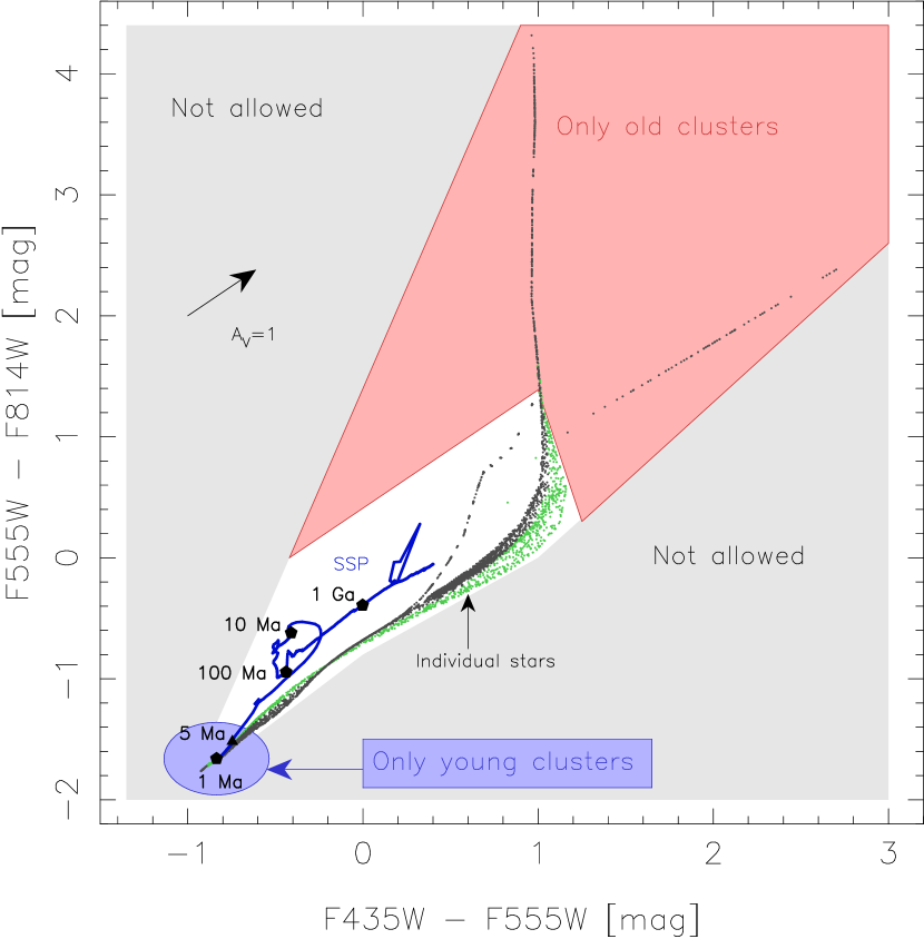
Figure 7: Graphical representation of the boundary conditions. The blue track shows the evolution of well-populated SSP models (from the bottom-left corner of the figure to redder colours as a function of increasing age). The black pentagrams highlight SSPs of ages as indicated. The red area defines the region within which only old ($\geq 10^{8}$ yr) clusters can reside; similarly, the blue area encompasses the region where we expect only young ($\leq 5$ Myr-old) clusters. The black dots show the positions of extremely underpopulated clusters (i.e., ‘clusters’ composed of single stars, based on the isochrones discussed in Section 3.1). The green dots represent stars with luminosities below those of the clusters in our sample, whereas the grey dots are stars that are more luminous than our clusters (in any filter). The grey-shaded areas cannot host any clusters, since there is no possible combination of single stars that can produce such cluster colours (see the text for details). The extinction vector for $A_{V}=1$ mag is shown for reference.

Since we are in a situation where not all stars defining the isochrone may be present in the cluster, we are bound by a number of additional rules. In essence, we need to work with the general considerations outlined above, but we also need to take into account only those stars that would be present in the cluster. This leads to two basic rules.

1. Only individual stars less luminous than the cluster may be considered in order to define the region in colour-colour space where a cluster of a given age could reside.

2. No cluster can have colours that are not covered by either the individual stars or the SSP models.

3.4 Application of the LLL test

In Fig. 8 we show the colour-colour diagram of the observed clusters in the M82 nucleus. We have also included the positions of the SSP models and of individual stars for a foreground extinction of $A_{V}=0$ and 4 mag, respectively. For $A_{V}=0$ mag, it appears that most of the clusters can be explained by an old age ($\ga 10^{8}$ yr). However, if we take into account the limitation imposed by the cluster luminosities, none of these clusters can host stars more massive than 6 M_⊙, and the extreme $(B-V)$ and $(V-I)$ values are $\sim$1 mag. In this situation, neither clusters redder than $(B-V)=1$ mag, nor those redder than the $(V-I)$ values defined by the SSP models can be explained. This implies that at least some amount of extinction is required to match the distribution of the clusters in colour-colour space.

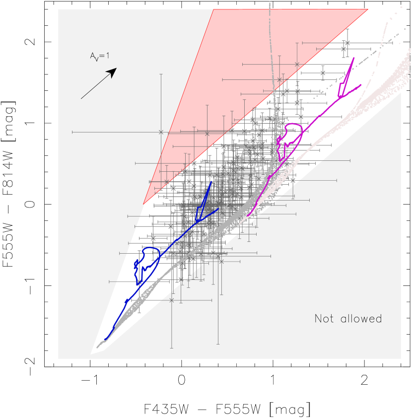
Figure 8: Observed colour-colour diagram for the nuclear clusters in M82. The blue and purple tracks show the evolution of SSP models affected by $A_{V}=0$ and 4 mag, respectively; the dark and light-grey dots represent the colours of individual stars affected by similar extinction values. The red shaded area is the region where we would expect only older ($\geq 10^{8}$ yr) clusters to be found; the extinction vector for $A_{V}=1$ mag is shown for reference.

For $A_{V}=4$ mag, the model curve seems to imply that all clusters are young ($\leq 5$ Myr old). However, this choice of extinction value cannot explain any cluster with $(B-V)<0.5$ mag, for which less extinction would be required.

Whatever the case, clusters that are redder in $(V-I)$ than the envelope of the SSP models with variable extinction (i.e., those redder than a line with a slope $\ga 1$), are most likely explained by the presence of individual stars in the $(V-I)$ tail at $(B-V)=1$ mag for $A_{V}=0$ mag. This tail corresponds to stars older than 100 Myr and, hence, these are ‘old’ clusters. In this case, a moderate amount of extinction is needed if the clusters are to host such luminous red stars. However, we note that in view of the significant photometric uncertainties, some of the observed redder clusters could be consistent with younger clusters ($\sim 10^{7}$–$10^{8}$ yr old) affected by varying amounts of extinction.

3.5 Application of standard SSP analysis

Although we are clearly aware of the IMF sampling issues discussed in the previous section, we will now apply the ‘standard’ SSP analysis to our cluster photometry, in order to show what effects ignoring IMF sampling effects would have on the derived results. In other words, we will simply obtain the cluster ages (and their masses) assuming that their IMFs are well populated, without resorting to the LLL test discussed above. This will give us a good handle on the age uncertainties introduced by ignoring IMF sampling effects, which we will highlight where appropriate and relevant.

3.6 Age and mass distributions

In a series of recent papers, we developed a sophisticated tool for star cluster analysis based on broad-band SEDs, AnalySED, which we tested extensively both internally (de Grijs et al. 2003a,b; Anders et al. 2004b) and externally (de Grijs et al. 2005), using both theoretical and observed young to intermediate-age ($\lesssim 3\times 10^{9}$ yr) star cluster SEDs, and the galev SSP models (Kurth et al. 1999; Schulz et al. 2002). The accuracy has been further increased for younger ages by the inclusion of an extensive set of nebular emission lines, as well as gaseous continuum emission (Anders & Fritze-von Alvensleben 2003). We concluded that the relative ages and masses within a given cluster system can be determined to a very high accuracy, depending on the specific combination of passbands used (Anders et al. 2004b). Even when comparing the results of different groups using the same data set, we can retrieve any prominent features in the cluster age and mass distributions to within $\Delta\langle\log({\rm Age/yr})\rangle\leq 0.35$ and $\Delta\langle\log(M_{\rm cl}/{\rm M}_{\odot})\rangle\leq 0.14$, respectively (de Grijs et al. 2005), which confirms that we understand the uncertainties associated with the use of our AnalySED tool to a very high degree – provided that our sample clusters have well-populated IMFs.

We therefore applied the AnalySED approach to our full set of broad-band $UBVI$ cluster SEDs (we note that $U$-band photometry is only available for a subset of 127 clusters), assuming a Kroupa (2001) IMF (with a low-mass cut-off at 0.1 M_⊙) and Padova isochrones. Four-passband photometry is, in general, sufficient to yield robust cluster parameters with reasonable uncertainties (Anders et al. 2004b). However, given the highly variable galactic background in our field of view (see Fig. 1), we decided to fix the model cluster metallicities to the solar value, leaving both the cluster ages and extinction values as free parameters. The shape of the broad-band SEDs constrains the ages and extinction values, whereas the absolute flux level results in the corresponding cluster masses. Despite the significant photometric uncertainties, generally caused by the highly variable background, our SED matching approach was fairly successful in converging to a reasonably well-determined set of ages: of the 152 cluster candidates selected, we obtained ages for 142.

Figure 9: (top left and bottom left) Age and mass distributions of the clusters in the M82 starburst core, based on the straightforward application of SED matching using standard SSP models; (top right and bottom right: Full ($1\sigma$) uncertainty ranges in age and mass, as a function of cluster age and mass, respectively. See the text for details.

The resulting histogram of the best-fitting cluster ages is shown in the top left-hand panel of Fig. 9. The cluster age distribution shows a peak around log( Age / yr ) $\sim 9$, with a broad distribution (of order 40% of the sample clusters) extending towards younger ages. Whether or not the apparent peak(s) at younger ages is (are) real depends on the uncertainties in our age estimates. The AnalySED output also provides realistic ($1\sigma$) uncertainty estimates (see Anders et al. 2004b). In the top right-hand panel of Fig. 9 we visualise the full uncertainty ranges for all our clusters, as a function of age. We emphasise that these uncertainties represent the full range from the minimum to the maximum ages allowed by the fitting routines; because of the logarithmic representation, we note that the uncertainty ranges are asymmetrical, however, so that it is impractical to show average values. As an aside, we also note that our results are not dominated by the age-extinction degeneracy inherent to the use of broad-band photometry, given that there is no discernible trend between the resulting cluster ages and their extinction values (a trend would be expected if this degeneracy were important). The use of both the $U$-band filter and a red optical passband ($I$) minimises any residual age-extinction degeneracy (e.g., Anders et al. 2004b).

We will now use these uncertainty estimates to provide an independent cross-check on the accuracy of our age determinations. Cluster A1 was found to have an age of $5.2\pm 1.5$ Myr (and $E(B-V)=0.85^{+0.05}_{-0.65}$ mag), which is – given the uncertainties – in good agreement with the age estimate of $6.4\pm 0.5$ Myr of Smith et al (2006), based on spectroscopy and for an extinction of $E(B-V)=1.35\pm 0.15$ mag. For cluster B2-1 (de Grijs et al. 2001; Smith et al. 2006), the age derived here ($2.0\pm 1.0$ Gyr; for $E(B-V)=0.60^{+0.10}_{-0.20}$ mag) is also consistent with previous age determinations: Smith et al. (2006) derived $\log(\mbox{Age yr}^{-1})=8.54\pm 0.8$ for $E(B-V)=0.97\pm 0.51$ mag (see also Smith et al. 2007), while de Grijs et al. (2001, 2003c) obtained $\log(\mbox{Age yr}^{-1})=9.7$–9.76 based on a small to negligible amount of extinction.

For completeness, the bottom left-hand panel of Fig. 9 shows the corresponding mass distribution of the nuclear M82 clusters in our sample. This shows that there is a broad distribution of cluster masses around $10^{5}$ M_⊙, not too dissimilar to the cluster mass distribution in the post-starburst region ‘B’ some 0.5–1.0 kpc from the centre of M82 (e.g., de Grijs et al. 2001, 2003c). Although there is a non-negligible fraction of clusters more massive than $\sim 10^{6}$ M_⊙ (which may, hence, qualify as SSCs), there is also a significant complement of fairly low-mass objects, down to $\sim 10^{3}$ M_⊙. The bottom right-hand panel shows the full mass ranges obtained for our sample clusters from the AnalySED fits, in a similar visualisation as shown in the top right-hand panel for the age uncertainties. A quick comparison of the general differences between both right-hand panels shows that, indeed, the average uncertainties in the cluster masses are relatively smaller than those for the ages, at least for masses $\ga 10^{5}$ M_⊙ (in support of de Grijs et al. 2005).

3.7 Constraints from H$\alpha$ imaging

We are fortunate in also having obtained an H$\alpha$ image of the galaxy’s starburst core. The addition of H$\alpha$ photometry allows us to determine the number of sample clusters showing an H$\alpha$ excess, which in turn will help us to constrain the cluster ages to $\la 8$ Myr. Of the 152 clusters in our sample, nineteen show a clear H$\alpha$ excess exceeding the 1$\sigma$ photometric uncertainties of the clusters’ total H$\alpha$ flux. This relatively small number does not necessarily imply that most objects are faint in H$\alpha$ flux, but rather that the photometric uncertainties are generally significant due to the highly variable background (see Fig. 1). For those clusters with a statistically significant H$\alpha$ excess, the corresponding ages based on their broad-band SEDs are in all cases consistent with them being younger than $\sim 10$ Myr.

Of these 19 clusters with a significant H$\alpha$ excess, twelve are located in or near region C. This is consistent with the observation that region C might be the youngest part of the starburst (Section 2.2), although our age resolution does not allow us to conclude this robustly; for all practical purposes, we may assume that regions A and C are of similar (young) age (see also O’Connell & Mangano 1978; O’Connell et al. 1995). Alternatively, region C may represent the actual core region generating the minor-axis H$\alpha$ ‘plume’ coincident with the minor-axis ‘superwind’ (cf. McCarthy et al. 1987; O’Connell et al. 1995; Westmoquette et al. 2007b). The right-hand panel of Fig. 4 shows the distribution of the H$\alpha$ excess across the entire region. In this representation, region C clearly stands out in H$\alpha$ emission, so it may indeed be the youngest core region.

4 Summary and Discussion

We have presented high-resolution HST/ACS imaging in four filters (Johnson-Cousins equivalent $B,V$, and $I$ broad bands, and an H$\alpha$ narrow-band filter), as well as subsequently acquired $U$-band images, of the nuclear starburst region of M82. The high spatial resolution of the HST images has allowed us to explore the central area of this galaxy in unparalleled detail. We find a complex system of $\sim$150 star clusters in the inner few 100 pc of M82, encompassing sections A, C, D, and E (O’Connell & Mangano 1978). At face value, the resulting cluster age distribution gives us a strong handle on the global star cluster formation intensity across the galaxy’s core region, which can then be compared to the field-star formation history.

As the archetypal local starburst galaxy, M82 is believed to have undergone a tidal interaction with its neighbour, M81, $\sim 10^{8}$ yr ago (e.g., Gottesman & Weliachew 1977; O’Connell & Mangano 1978; Lo et al. 1987; Yun et al. 1993, 1994), providing the means of activation of the intense episodes of starburst activity witnessed in M82. It has been suggested that this interaction led to the ISM of M82 experiencing large-scale torques, coupled with a loss of angular momentum as it was transferred towards the dynamical centre of the galaxy (FS03; also based on numerical simulations: e.g., Sundelius et al. 1987; Noguchi 1987, 1988; Mihos & Hernquist 1996). This led to an increased cloud-cloud collision rate in the disk of the galaxy, and large amounts of material accumulating and undergoing compression in the innermost regions, perhaps resulting in the first starburst episode (FS03).

We find (tentative) evidence of an enhanced cluster-formation epoch associated with the first starburst event (although we caution that the age uncertainties are significant), believed to have occurred about 100 Myr ago (or possibly as recently as $\sim 30$ Myr ago; Rieke et al. 1993). We do not find any strong evidence of enhanced star cluster formation at an age of $\sim 5$ Myr, however, believed to be the epoch when the more recent starburst event transpired in the region (FS03; supported by Smith et al. 2006). Perhaps this is due to the relatively small region studied here, in that it could be possible that the clusters analysed are not spatially associated with the more recent starburst event.

Förster Schreiber et al. (2003) indeed suggest that the two events took place in different regions, with the first happening in the centre of M82 and the second occurring predominantly in a circumnuclear ring and along the stellar bar. Alternatively, it could be the case that cluster formation is not always coincident with enhanced star-formation episodes. This type of scenario is, in fact, not unreasonable to expect, as evidenced by, e.g., the observed disparities between the cluster and field-star age distributions in the Magellanic Clouds and in NGC 1569 (see Anders et al. 2004a for a discussion regarding the latter galaxy). In particular, the Large Magellanic Cloud exhibits a well-known gap in the cluster age distribution, yet the age distribution of the field stellar population appears more continuous; the field-star and cluster formation histories are clearly very different (e.g., Olszewski et al. 1996; Geha et al. 1998; Sarajedini 1998; and references therein). Although the case is less clear-cut for the Small Magellanic Cloud, Rafelski & Zaritsky (2005) provide tentative evidence that the cluster and field-star age distributions are also significantly different in this system (see also Gieles et al. 2007).

We caution, however, that our cluster age estimates may be severely affected by IMF stochasticity, given that the luminosities of most of our sample clusters imply that their mass functions are not fully sampled up to the most luminous stars included in the theoretical stellar isochrones. We show the effects of statistical IMF sampling issues in colour-colour space. This should be taken as a strong warning to anyone (including ourselves) attempting to apply standard SSP analysis to integrated cluster photometry of any but the most massive star clusters. As a consequence, the age estimates derived based on standard SSP analysis should be taken with extreme caution. It is most likely that our straightforward SSP-based age determinations are affected by (i) residual effects due to the age-extinction degeneracy, despite the availability of $U$-band and H$\alpha$ observations, and – more importantly – (ii) significant stochastic effects.

It is our intention that this paper be taken by the community as a strong warning to consider stochasticity in the IMF for young clusters with undersampled stellar mass functions much more seriously than has been done to date (including by ourselves; e.g., de Grijs et al. 2003a,b).

References

- Anders & Fritze-von Alvensleben (2003) Anders, P., & Fritze-von Alvensleben, U. 2003, A&A, 401, 1063
- Anders et al. (2004) Anders, P., de Grijs, R., Fritze-von Alvensleben, U., & Bissantz, N. 2004a, MNRAS, 347, 17
- Anders et al. (2004) Anders, P., Bissantz, N., Fritze-von Alvensleben, U., & de Grijs, R. 2004b, MNRAS, 347, 196
- Anders, Gieles, & de Grijs (2006) Anders, P., Gieles, M., & de Grijs, R. 2006, A&A, 451, 375
- Arp & Sandage (1985) Arp, H., & Sandage, A. 1985, AJ, 90, 1163
- (6) Bastian N., Gieles M., Lamers H.J.G.L.M., Scheepmaker R.A., de Grijs R., 2005, A&A, 431, 905
- Bertelli et al. (1994) Bertelli, G., Bressan, A., Chiosi, C., Fagotto, F., & Nasi, E. 1994, A&AS, 106, 275
- Brouillet et al. (1991) Brouillet, N., Baudry, A., Combes, F., Kaufman, M., & Bash, F. 1991, A&A, 242, 35
- Bruhweiler, Miskey, & Smith Neubig (2003) Bruhweiler, F. C., Miskey, C. L., & Smith Neubig M. 2003, AJ, 125, 3082
- Cardelli, Clayton, & Mathis (1989) Cardelli, J. A., Clayton, G. C., & Mathis, J. S. 1989, ApJ, 345, 245
- Carlson et al. (1998) Carlson, M. N., Holtzman, J. A., Watson, A. M., et al. 1998, AJ, 115, 1778
- Cerviño, Luridiana, & Castander (2000) Cerviño, M., Luridiana, V., & Castander, F. J. 2000, A&A, 360, L5
- Cerviño et al. (2001) Cerviño, M., Gómez-Flechoso, M. A., Castander, F. J., et al. 2001 A&A, 376, 422
- Cerviño et al. (2002) Cerviño, M., Valls-Gabaud, D., Luridiana, V., & Mas-Hesse, J. M. 2002, A&A, 381, 51
- Cerviño & Luridiana (2004) Cerviño, M., & Luridiana, V. 2004, A&A, 413, 145
- Cerviño & Luridiana (2006) Cerviño, M., & Luridiana, V. 2006, A&A, 451, 475
- Cerviño & Valls-Gabaud (2008) Cerviño, M. Valls-Gabaud, D. 2008, in: Young massive star clusters – Initial conditions and environments, eds. E. Pérez, R. de Grijs, & R. M. González Delgado, Springer: Dordrecht, in press (arXiv:0802.3213v1)
- Conti, Leitherer, & Vacca (1996) Conti, P. S., Leitherer, C., & Vacca, W. D. 1996, ApJ, 461, L87
- de Grijs et al. (2000) de Grijs, R., O’Connell, R. W., Becker, G. D., Chevalier, R. A., & Gallagher, J. S., iii 2000, AJ, 119, 681
- de Grijs, O’Connell, & Gallagher (2001) de Grijs, R., O’Connell, R. W., & Gallagher, J. S., iii 2001, AJ, 121, 768
- de Grijs et al. (2003) de Grijs, R., Anders, P., Bastian, N., et al. 2003a, MNRAS, 343, 1285
- de Grijs et al. (2003) de Grijs, R., Fritze-von Alvensleben, U., Anders, P., et al. 2003b, MNRAS, 342, 259
- de Grijs, Bastian, & Lamers (2003) de Grijs, R., Bastian, N., & Lamers, H. J. G. L. M. 2003c, ApJ, 583, L17
- de Grijs et al. (2005) de Grijs, R., Anders, P., Lamers, H. J. G. L. M., et al. 2005, MNRAS, 359, 874
- de Grijs & Parmentier (2007) de Grijs, R., & Parmentier, G. 2007, ChJAA, 7, 155
- Fabbiano & Trinchieri (1984) Fabbiano, G., & Trinchieri, G. 1984, ApJ, 286, 491