Radial temperature profiles for a large sample of galaxy clusters observed with XMM-Newton

Abstract

Aims. We measure, as far out as possible, radial temperature profiles for a sample of $\approx 50$ hot, intermediate redshift galaxy clusters, selected from the XMM-Newton archive, keeping systematic errors under control.

Methods. Our work is characterized by two major improvements. Firstly, we use the background modeling, rather than the background subtraction, and the Cash statistic rather than the $\chi^{2}$; this method requires a careful characterization of all background components. Secondly, we assess in details systematic effects. We perform two groups of test: prior to the analysis, we make use of extensive simulations to quantify the impact of different spectral components on simulated spectra; after the analysis, we investigate how the measured temperature profile changes, when choosing different key parameters.

Results. The mean temperature profile declines beyond 0.2 $R_{180}$; for the first time we provide an assessment of the source and the magnitude of systematic uncertainties. When comparing our profile with that obtained from hydrodynamic simulations, we find the slopes beyond $\approx$ 0.2 $R_{180}$ to be similar. Our mean profile is similar but somewhat flatter with respect to that obtained by previous observational works, possibly as a consequence of a different level of characterization of systematic effects.

Conclusions. This work allows us not only to constrain with confidence cluster temperature profiles in outer regions, but also, from a more general point of view, to explore the limits of the current X-ray experiments (in particular XMM-Newton) with respect to the analysis of low surface brightness emission.

1 Introduction

Clusters of galaxies are the most massive gravitationally bound systems in the universe. They are permeated by the hot, X-ray emitting, intra-cluster medium (ICM), which represents the dominant baryonic component. The key ICM observable quantities are its density, temperature, and metallicity. Assuming hydrostatic equilibrium, the gas temperature and density profiles allow us to derive the total cluster mass and thus to use galaxy clusters as cosmological probes (e.g. Henry & Arnaud, 1991; Ettori et al., 2002; Fabian & Allen, 2003; Voit, 2005). Temperature and density profiles can also be combined to determine the ICM entropy distribution, that provides valuable information on the cluster thermodynamic history and has proven to be a powerful tool to investigate non-gravitational processes (e.g. Ponman et al., 2003; McCarthy et al., 2004; Voit, 2005; Pratt et al., 2006).

Cluster outer regions are rich of information and interesting to study, because clusters are still forming there by accretion (e.g. Tozzi et al., 2000; Borgani et al., 2004); moreover, far from the core it is easier to compare simulations with observations, because feedback effects are less important (e.g. Borgani et al., 2004; McNamara et al., 2005; Roncarelli et al., 2006). Cluster surface brightness rapidly declines with radius, while background (of instrumental, solar, local, and cosmic origin) is roughly constant over the detector. For this reason, spectra accumulated in the outer regions are characterized by poor statistics and high background, especially at high energies, where the instrumental background dominates other components. These conditions make temperature measurement at large distances from the center a technically challenging task, requiring an adequate treatment of both statistical and systematic issues (Leccardi & Molendi, 2007).

Given the technical difficulties, early measurements of cluster temperature profiles have been controversial. At the end of the ASCA and BeppoSAX era, the shape of the profiles at large radii was still the subject of debate (Markevitch et al., 1998; Irwin et al., 1999; White, 2000; Irwin & Bregman, 2000; Finoguenov et al., 2001; De Grandi & Molendi, 2002). Recent observations with current experiments (i.e. XMM-Newton and Chandra) have clearly shown that cluster temperature profiles decline beyond the 15-20% of R₁₈₀ (Piffaretti et al., 2005; Vikhlinin et al., 2005; Pratt et al., 2007; Snowden et al., 2008). However, most of these measurements might be unreliable at very large radii ($\gtrsim$ 50% of R₁₈₀) because they are affected by a number of systematics related to the analysis technique and to the background treatment (Leccardi & Molendi, 2007).

The aim of this work is to measure the mean temperature profile of galaxy clusters as far out as possible, while keeping systematic errors under control. We select from the XMM-Newton archive all hot ($\mathrm{k}T>3.5$ keV), intermediate redshift ($0.1\lesssim z\lesssim 0.3$) clusters, that are not strongly interacting, and measure their radial temperature profiles. The spectral analysis follows a new approach: we use the background modeling, rather than the background subtraction, and the Cash statistic rather than the $\chi^{2}$. This method requires a careful characterization (reported in the Appendices) of all background components, which unfortunately has not been possible for EPIC-pn; for this reason, in our analysis we use only EPIC-MOS data.

Background parameters are estimated in a peripheral region, where the cluster emission is almost negligible, and rescaled in the regions of interest. The spectral fitting is performed in the 0.7-10.0 keV and in the 2.0-10.0 keV energy bands, that are characterized by different statistics and level of systematics, to check the consistency of our results. A second important point is a particular attention to systematic effects. We perform two groups of test: prior to the analysis, we make use of extensive simulations to quantify the impact of different components (e.g. the cosmic variance or the soft proton contribution) on simulated spectra; after the analysis, we investigate how the measured temperature profile changes, when choosing different key parameters (e.g. the truncation radius or the energy band). At the end of our tests, we provide an assessment of the source and the magnitude of systematic uncertainties associated to the mean profile.

We compare our profiles with those obtained from hydrodynamic simulations (Borgani et al., 2004) and from previous observational works (De Grandi & Molendi, 2002; Vikhlinin et al., 2005; Pratt et al., 2007). Our work does not only provide a confirmation of previous results. For the first time we believe we know where the systematics come from and how large they are. Indeed, this work allows us not only to constrain with confidence cluster temperature profiles in the outer regions, but also, from a more general point of view, to explore the limits of the current X-ray experiments (in particular XMM-Newton). It is crucial that we learn how best to exploit XMM-Newton data, because for the next 5-10 years there will be no experiments with comparable or improved capabilities, as far as low surface brightness emission is concerned. Our work will also allow us to look forward to ambitious new measurements: an example is the attempt to measure the putative shock in Abell 754, for which we have obtained a $\approx 200$ ks observation with XMM-Newton in AO7.

The outline of the paper is the following. In Sect. 2 we describe sample properties and selection criteria and in Sect. 3 we describe in detail our data analysis technique. In Sect. 4 we present the radial temperature profiles for all clusters in our sample and compute the average profile. In Sect. 5 we describe our analysis of systematic effects. In Sect. 6 we characterize the profile decline, investigate its dependency from physical properties (e.g. the redshift), and compare it with hydrodynamic simulations and previous observational works. Our main results are summarized in Sect. 7. In the Appendices we report the analysis of closed and blank field observations, which allows us to characterize most background components.

Quoted confidence intervals are 68% for one interesting parameter (i.e. $\Delta$C = 1), unless otherwise stated. All results are given assuming a $\Lambda$CDM cosmology with $\Omega_{\mathrm{m}}=0.3$, $\Omega_{\Lambda}=0.7$, and $H_{0}$ = 70 km s^-1 Mpc^-1.

2 The sample

We select from the XMM-Newton archive a sample of hot ($\mathrm{k}T>3.3$ keV), intermediate redshift ($0.1\lesssim z\lesssim 0.3$), and high galactic latitude ($|b|>20^{\circ}$) clusters of galaxies. Upper and lower limits to the redshift range are determined, respectively, by the cosmological dimming effect and the size of the EPIC field of view ($\approx 15^{\prime}$ radius). Indeed, our data analysis technique requires that the intensity of background components be estimated in a peripheral region, where the cluster emission is almost negligible (see Sect. 3.2.1). We retrieve from the public archive all observations of clusters satisfying the above selection criteria, performed before March 2005 (when the CCD6 of EPIC-MOS1 was switched off) and available at the end of May 2007.

Table 1: Observations excluded from the sample due to high soft proton contamination.

Name	Obs ID
RXCJ0303.8-7752	0042340401
RXCJ0516.7-5430	0042340701
RXCJ0528.9-3927	0042340801
RXCJ2011.3-5725	0042341101
Abell 2537	0042341201
RXCJ0437.1+0043	0042341601
Abell 1302	0083150401
Abell 2261	0093030301
Abell 2261	0093030801
Abell 2261	0093030901
Abell 2261	0093031001
Abell 2261	0093031101
Abell 2261	0093031401
Abell 2261	0093031501
Abell 2261	0093031601
Abell 2261	0093031801
Abell 2219	0112231801
Abell 2219	0112231901
RXCJ0006.0-3443	0201900201
RXCJ0145.0-5300	0201900501
RXCJ0616.8-4748	0201901101
RXCJ0437.1+0043	0205330201
Abell 2537	0205330501

Unfortunately, 23 of these 86 observations are highly affected by soft proton flares (see Table 1). We exclude them from the sample, because their good (i.e. after flare cleaning, see Sect. 3.1.1) exposure time is not sufficient (less than 16 ks when summing MOS1 and MOS2) to measure reliable temperature profiles out to external regions.

Table 2: Observations of clusters that show evidence of recent and strong interactions.

Name	Obs ID
Abell 2744	0042340101
Abell 665	0109890401
Abell 665	0109890501
Abell 1914	0112230201
Abell 2163	0112230601
Abell 2163	0112231501
RXCJ0658.5-5556	0112980201
Abell 1758	0142860201
Abell 1882	0145480101
Abell 901	0148170101
Abell 520	0201510101
Abell 2384	0201902701
Abell 115	0203220101
ZwCl2341.1+0000	0211280101

Furthermore, we exclude 14 observations of clusters that show evidence of recent and strong interactions (see Table 2). For such clusters, a radial analysis is not appropriate, because the gas distribution is far from being azimuthally symmetric. Finally, we find that the target of observation 0201901901, which is classified as a cluster, is likely a point-like source; therefore, we exclude this observation too from our sample.

Table 3: Physical properties and observation details for the 48 clusters of our sample.

Name	Obs ID	$z\mathrm{{}^{a}}$	$\mathrm{k}T_{\mathrm{M}}\mathrm{{}^{b}}$	$R_{180}\mathrm{{}^{c}}$	Exp. timed		$R_{\mathrm{SB}}\mathrm{{}^{e}}$	Filter
RXCJ0043.4-2037	0042340201	0.2924	6.8	1.78	11.9	11.3	1.25	THIN1
RXCJ0232.2-4420	0042340301	0.2836	7.2	1.85	12.1	11.7	1.08	THIN1
RXCJ0307.0-2840	0042340501	0.2534	6.8	1.82	11.4	12.6	1.08	THIN1
RXCJ1131.9-1955	0042341001	0.3072	8.1	1.93	12.4	12.3	1.08	THIN1
RXCJ2337.6+0016	0042341301	0.2730	7.2	1.86	13.4	13.1	1.19	THIN1
RXCJ0532.9-3701	0042341801	0.2747	7.5	1.90	10.9	10.5	1.09	THIN1
Abell 68	0084230201	0.2550	7.2	1.88	26.3	25.9	1.37	MEDIUM
Abell 209	0084230301	0.2060	6.6	1.85	17.9	17.8	1.19	MEDIUM
Abell 267	0084230401∗	0.2310	4.5	1.49	17.0	16.5	1.79	MEDIUM
Abell 383	0084230501	0.1871	4.4	1.52	29.3	29.8	1.33	MEDIUM
Abell 773	0084230601	0.2170	7.5	1.96	13.6	15.5	1.16	MEDIUM
Abell 963	0084230701	0.2060	6.5	1.83	24.4	26.0	1.19	MEDIUM
Abell 1763	0084230901	0.2230	7.2	1.92	13.0	13.2	1.08	MEDIUM
Abell 1689	0093030101	0.1832	9.2	2.21	36.8	36.8	1.14	THIN1
RX J2129.6+0005	0093030201	0.2350	5.5	1.66	36.0	37.5	1.21	MEDIUM
ZW 3146	0108670101	0.2910	7.0	1.81	52.9	52.9	1.07	THIN1
E1455+2232	0108670201	0.2578	5.0	1.56	35.3	35.8	1.11	MEDIUM
Abell 2390	0111270101	0.2280	11.2	2.37	9.9	10.3	1.11	THIN1
Abell 2204	0112230301	0.1522	8.5	2.16	18.2	19.5	1.06	MEDIUM
Abell 1413	0112230501	0.1427	6.7	1.92	25.4	25.4	1.10	THIN1
Abell 2218	0112980101	0.1756	6.5	1.86	18.2	18.2	1.17	THIN1
Abell 2218	0112980401	0.1756	7.0	1.93	13.7	14.0	1.42	THIN1
Abell 2218	0112980501	0.1756	6.1	1.80	11.3	11.0	1.07	THIN1
Abell 1835	0147330201	0.2532	8.6	2.05	30.1	29.2	1.16	THIN1
Abell 1068	0147630101	0.1375	4.5	1.58	20.5	20.8	1.09	MEDIUM
Abell 2667	0148990101	0.2300	7.7	1.96	21.9	21.6	1.48	MEDIUM
Abell 3827	0149670101	0.0984	7.1	2.02	22.3	22.4	1.16	MEDIUM
Abell 3911	0149670301	0.0965	5.4	1.77	25.8	26.1	1.43	THIN1
Abell 2034	0149880101	0.1130	7.0	1.99	10.2	10.5	1.16	THIN1
RXCJ0003.8+0203	0201900101	0.0924	3.7	1.47	26.3	26.6	1.10	THIN1
RXCJ0020.7-2542	0201900301	0.1424	5.7	1.78	14.8	15.4	1.02	THIN1
RXCJ0049.4-2931	0201900401	0.1080	3.3	1.37	19.2	18.8	1.28	THIN1
RXCJ0547.6-3152	0201900901	0.1483	6.7	1.92	23.3	24.0	1.12	THIN1
RXCJ0605.8-3518	0201901001	0.1410	4.9	1.65	18.0	24.1	1.07	THIN1
RXCJ0645.4-5413	0201901201	0.1670	7.1	1.95	10.9	10.9	1.11	THIN1
RXCJ1044.5-0704	0201901501	0.1323	3.9	1.47	25.7	25.9	1.03	THIN1
RXCJ1141.4-1216	0201901601	0.1195	3.8	1.46	28.4	28.6	1.03	THIN1
RXCJ1516.3+0005	0201902001	0.1183	5.3	1.73	26.7	26.6	1.13	THIN1
RXCJ1516.5-0056	0201902101	0.1150	3.8	1.46	30.0	30.0	1.08	THIN1
RXCJ2014.8-2430	0201902201	0.1612	7.1	1.96	23.0	23.4	1.05	THIN1
RXCJ2048.1-1750	0201902401	0.1470	5.6	1.75	24.6	25.3	1.07	THIN1
RXCJ2149.1-3041	0201902601	0.1179	3.3	1.37	25.1	25.5	1.11	THIN1
RXCJ2218.6-3853	0201903001	0.1379	6.4	1.88	20.2	21.4	1.11	THIN1
RXCJ2234.5-3744	0201903101	0.1529	8.6	2.17	18.9	19.3	1.31	THIN1
RXCJ0645.4-5413	0201903401	0.1670	8.5	2.13	11.5	12.1	1.51	THIN1
RXCJ0958.3-1103	0201903501	0.1527	6.1	1.83	8.3	9.4	1.16	THIN1
RXCJ0303.8-7752	0205330101	0.2742	7.5	1.89	11.7	11.5	1.18	THIN1
RXCJ0516.7-5430	0205330301	0.2952	7.5	1.87	11.4	11.7	1.19	THIN1

• ^a redshift taken from the NASA Extragalactic Database; ^b mean temperature in keV derived from our analysis; ^c scale radius in Mpc derived from our analysis; ^d MOS1 and MOS2 good exposure time in ks; ^e intensity of residual soft protons (see Eq. 1); ^∗ excluded due to high residual soft proton contamination.

In Table 3 we list the 48 observations that survived our selection criteria and report cluster physical properties. The redshift value (from optical measurements) is taken from the NASA Extragalactic Database; $\mathrm{k}T_{\mathrm{M}}$ and $R_{180}$ are derived from our analysis (see Sect. 4).

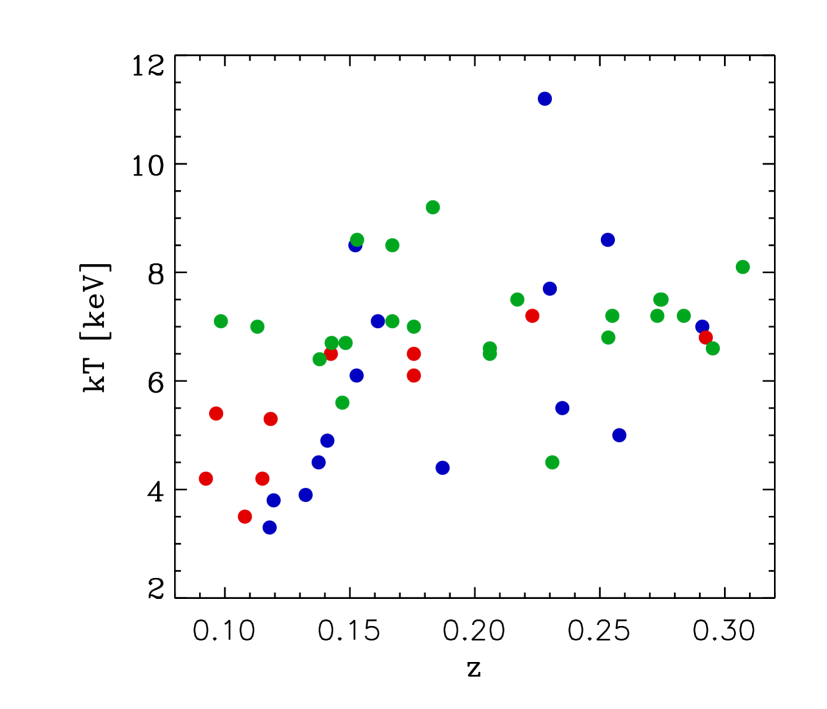
Figure 1: Distribution of selected clusters in the redshift-temperature space. We distinguish cool core (blue), non cool core (red) and uncertain (green) clusters, as defined in Sect. 6. There is no evidence of selection effects, except for a weak positive correlation between redshift and temperature.

In Fig. 1 we report the cluster distribution in the redshift-temperature space. The only selection effect we detect is the paucity of cool ($\mathrm{k}T_{\mathrm{M}}\lesssim 5$ keV) clusters at high ($z>0.2$) redshift. Observations are performed with THIN1 and MEDIUM filters, as reported in Table 3.

3 Data analysis

The preparation of spectra comprises the following major steps:

• preliminary data processing;

• good time interval (GTI) filtering to exclude periods of high soft proton flux;

• filtering according to pattern and flag criteria;

• excision of brightest point-like sources;

• calculation of the “IN over OUT” ratio;

• extraction of spectra in concentric rings.

The spectral analysis is structured as follows:

• estimate of background parameters from a peripheral ring of the field of view;

• spectral fitting using the Cash statistic and modeling the background, rather than subtracting it, as commonly done;

• production of surface brightness, temperature, and metallicity profiles.

All these points are described in detail in the following subsections.

In our analysis we use only EPIC-MOS data, because a robust characterization of EPIC-pn background has not been possible, mainly due to the small regions outside the field of view and to the non-negligible fraction of out of time events (for further details, see Appendix B). Moreover, the EPIC-pn background is less stable than the EPIC-MOS one, especially below 2 keV.

3.1 Spectra preparation

3.1.1 Preliminary data preparation

Observation data files (ODF) are retrieved from the XMM-Newton archive and processed in a standard way with the Science Analysis System (SAS) v6.1.

The soft proton cleaning is performed using a double filtering process. We extract a light curve in 100 second bins in the 10-12 keV energy band by excluding the central CCD, apply a threshold of 0.20 cts s^-1, produce a GTI file and generate the filtered event file accordingly. This first step allows to eliminate most flares, however softer flares may exist such that their contribution above 10 keV is negligible. We then extract a light curve in the 2-5 keV band and fit the histogram obtained from this curve with a Gaussian distribution. Since most flares have been rejected in the previous step, the fit is usually very good. We calculate the mean count rate, $\mu$, and the standard deviation, $\sigma$, apply a threshold of $\mu+3\sigma$ to the distribution, and generate the filtered event file.

After soft proton cleaning, we filter the event file according to PATTERN and FLAG criteria (namely PATTERN$\leq$12 and FLAG==0).

Figure 2: Histograms of the frequency distribution for averaged MOS exposure time (left panel) and $R_{\mathrm{SB}}$ (right panel) values.

In Table 3 we report the good exposure time after the soft proton cleaning; as mentioned in Sect. 2, we exclude observations for which the total (MOS1+MOS2) good exposure time is less than 16 ks. In the left panel of Fig. 2 we report the histogram of the frequency distribution for observation exposure times.

When fitting spectra in the 0.7-10.0 keV band (see Sect. 3.2), we also exclude the “bright” CCDs, i.e. CCD-4 and CCD-5 for MOS1 and CCD-2 and CCD-5 for MOS2 (see Appendix A for the discussion).

Brightest point-like sources are detected, using a procedure based on the SAS task edetect_chain and excluded from the event file. We estimate a flux limit for excluded sources in the order of $10^{-13}$ erg cm^-2 s^-1; after the source excision, the cosmic variance of the X-ray background on the entire field of view is $\approx$ 20%.

3.1.2 Quiescent soft proton contamination

A quiescent soft proton (QSP) component can survive the double filtering process (see Sect. 3.1.1). To quantify the amount of this component, we make use of the “IN over OUT” diagnostic (De Luca & Molendi, 2004). We measure the surface brightness, SB_IN, in an outer region of the field of view, where the cluster emission is negligible, and compare it to the surface brightness, SB_OUT, calculated outside the field of view in the same energy range (i.e. 6-12 keV). Since soft protons are channeled by the telescope mirrors inside the field of view and the cosmic ray induced background covers the whole detector, the ratio

$$R_{\mathrm{SB}}=\frac{S\!B_{\mathrm{IN}}}{S\!B_{\mathrm{OUT}}}$$ (1)

is a good indicator of the intensity of residual soft protons and is used for background modeling (see Sect. 3.2.2 and Appendix B). In Table 3 we report the values of $R_{\mathrm{SB}}$ for each observation; they roughly span the range between 1.0 (negligible contamination) and 1.5 (high contamination). The typical uncertainty in measuring $R_{\mathrm{SB}}$ is a few percent. In the right panel of Fig. 2 we report the frequency distribution for $R_{\mathrm{SB}}$ values. Since the observation 0084230401 of Abell 267 is extremely polluted by QSP ($R_{\mathrm{SB}}=1.8$), we exclude it from the sample.

3.1.3 Spectra accumulation

The cluster emission is divided in 10 concentric rings (namely 0^′-0.5^′, 0.5^′-1^′, 1^′-1.5^′, 1.5^′-2^′, 2^′-2.75^′, 2.75^′-3.5^′, 3.5^′-4.5^′, 4.5^′-6^′, 6^′-8^′, and 10^′-12^′). The center of the rings is determined by surface brightness isocontours at large radii and is not necessarily coincident with the X-ray emission peak. We prefer that azimuthal symmetry be preserved at large radii, where we are interested in characterizing profiles, at the expense of central regions.

For each instrument (i.e MOS1 and MOS2) and each ring, we accumulate a spectrum and generate an effective area (ARF); for each observation we generate one redistribution function (RMF) for MOS1 and one for MOS2. We perform a minimal grouping to avoid channels with no counts, as required by the Cash statistic.

3.2 Spectral analysis

Spectral fitting is performed within the XSPEC v11.3 package. The choice of the energy band for the spectral fitting is not trivial. We fit spectra in the 0.7-10.0 keV and in the 2.0-10.0 keV energy bands, by using the Cash statistic, with an absorbed thermal plus background model. The high energy band has the advantage of requiring a simplified background model (see Appendices A and B); however, the bulk of source counts is excluded and the statistical quality of the measurement is substantially reduced. Due to the paucity of source counts, there is a strong degeneracy between source temperature and normalization, and the temperature is systematically underestimated; therefore, when using the 2.0-10.0 keV band, an “a posteriori” correction is required (Leccardi & Molendi, 2007). On the contrary, in the 0.7-10.0 keV band, the statistical quality of the data is good, but the background model is more complicated and background components are less stable and affected by strong degeneracy (see Appendices A and B). We exclude the band below 0.7 keV because the shape of the internal background is very complicated and variable with time and because the source counts reach their maximum at $\approx$ 1 keV. Hereafter, all considerations are valid for both energy bands, unless otherwise stated.

In conditions of poor statistics (i.e. few counts/bin) and high background, the Cash statistic (Cash, 1979) is more suitable than the $\chi^{2}$ with reasonable channel grouping (Leccardi & Molendi, 2007). The Cash statistic requires the number of counts in each channel to be greater than zero (Cash, 1979); thus, the background cannot be subtracted. In our case the total background model is the sum of many components, each one characterized by peculiar temporal, spectral, and spatial variations (see Appendix B); when subtracting the background, the information on single components is lost. Conversely, background modeling allows to preserve the information and to manage all components appropriately. Moreover, we recall that the background modeling does not require strong channel grouping, error propagation, or renormalization factors.

3.2.1 Estimate of background parameters

To model the background, a careful characterization of all its components is mandatory. Ideally, one would like to estimate background parameters in the same region and at the same time as the source. Since this is not possible, we estimate background parameters in the external 10^′-12^′ ring and rescale them in the inner rings, by making reasonable assumptions on their spatial distribution tested by analyzing blank field observations (see Appendix B). The 10^′-12^′ ring often contains a weak cluster emission that, if neglected, may cause a systematic underestimate of temperature and normalization in the inner rings (see Sect. 5.1.2). In this ring the spectral components in the 0.7-10.0 keV band are:

• the thermal emission from the cluster (GCL),

• the emission from the Galaxy Halo (HALO),

• the cosmic X-ray background (CXB),

• the quiescent soft protons (QSP),

• the cosmic ray induced continuum (NXB),

• the fluorescence emission lines;

the HALO component is negligible when considering the 2.0-10.0 keV range. The model is the same used when analyzing blank field observations (see Appendix B for further details) plus a thermal component for the GCL.

We fixed most parameters (namely all except for the normalization of HALO, CXB, NXB, and fluorescence lines) to reduce the degeneracy due to the presence of different components with similar spectral shapes. All cluster parameters are fixed: the temperature, $\mathrm{k}T$, and the normalization, $N_{\mathrm{S}}$, are extrapolated from the final profiles through an iterative procedure; the metallicity, $Z$, is fixed to 0.2 solar (the solar abundances are taken from Anders & Grevesse (1989)) and the redshift, $z$, is fixed to the optical value. The QSP normalization, $N_{\mathrm{QSP}}$, is calculated from $R_{\mathrm{SB}}$ (see Appendix B) and fixed. Minor discrepancies in shape or normalization with respect to the real QSP spectrum are possible; the model accounts for them by slightly changing the normalization of other components, i.e. $N_{\mathrm{HALO}}$, $N_{\mathrm{CXB}}$, and $N_{\mathrm{NXB}}$ (for the discussion of the systematic effects related to QSP see Sects. 5.1.3 and 5.2.3).

Summarizing, in the 10^′-12^′ ring we determine the range of variability, [$N_{\mathrm{min}}$,$N_{\mathrm{max}}$], (i.e. the best fit value $\pm$1$\sigma$ uncertainty) for the normalization of the main background components, i.e. $N_{\mathrm{HALO}}$, $N_{\mathrm{CXB}}$, and $N_{\mathrm{NXB}}$. Once properly rescaled, this information allows us to constrain background parameters in the inner rings.

3.2.2 Spectral fit in concentric rings

We fit spectra in internal rings with the same model adopted in the 10^′-12^′ ring case (see Sect. 3.2.1). In Fig. 3 we compare spectra and best fit models for two different regions of the same cluster; in the inner ring (1^′-1.5^′) source counts dominate, while in the outer ring (4.5^′-6^′) background counts dominate.

Figure 3: Spectra and best fit models for the 1^′-1.5^′ (left) and the 4.5^′-6^′ (right) rings of Abell 1689. The solid thick and the dotted thick lines represent respectively the thermal and the total background model. The solid thin line represents the total (i.e. thermal + background) model. In the inner ring source counts dominate background ones, in the outer the opposite is true.

The equivalent hydrogen column density along the line of sight, $N_{\mathrm{H}}$, is fixed to the 21 cm measurement (Dickey & Lockman, 1990). Since clusters in our sample are at high galactic latitude ($|b|>20^{\circ}$), the $N_{\mathrm{H}}$ is $<10^{21}$ cm^-2 and the absorption effect is negligible above 1 keV. We always leave the temperature, $\mathrm{k}T$, and the normalization, $N_{\mathrm{S}}$, free to vary; the metallicity is free below $\approx$ 0.4 $R_{180}$ and fixed to 0.2 solar beyond; the redshift is allowed to vary between $\pm$7% of the optical measurement in the two innermost rings and, in the other rings, is fixed to the average value of the first two rings.

$N_{\mathrm{HALO}}$, $N_{\mathrm{CXB}}$, and $N_{\mathrm{NXB}}$ for the inner rings are obtained by rescaling the best-fit values in the 10^′-12^′ ring (see Sect. 3.2.1) by the area ratio and the correction factor, $K(r)$, obtained from blank field observations (see Table 8 in Appendix B):

$$N^{\mathrm{int}}=N^{\mathrm{ext}}\times\frac{Area^{\mathrm{int}}}{Area^{\mathrm{ext}}}\times K(r)\;,$$ (2)

for NXB $K=1$ for all rings. $N^{\mathrm{int}}_{\mathrm{HALO}}$, $N^{\mathrm{int}}_{\mathrm{CXB}}$, and $N^{\mathrm{int}}_{\mathrm{NXB}}$ are free to vary within a certain range: the lower (upper) limit of this range is derived by rescaling the best-fit value minus (plus) the 1$\sigma$-error calculated in the 10^′-12^′ ring. The local background should have a variation length scale of some degrees (Snowden et al., 1997); conversely, $N_{\mathrm{CXB}}$ may have large (i.e. 20-100%) variations between different rings due to the cosmic variance. However, extensive simulations show that these statistical fluctuations do not introduce systematics in the temperature measurement, when averaging on a large sample (see Sect. 5.1.1). $N^{\mathrm{int}}_{\mathrm{QSP}}$ is obtained by rescaling the value adopted in the 10^′-12^′ ring by the area ratio and by the QSP vignetting profile (Kuntz, 2006); $N^{\mathrm{int}}_{\mathrm{QSP}}$ is fixed for all rings. Normalizations of instrumental fluorescence emission lines are left free to vary within a limited range determined from the analysis of closed observations and have an almost negligible impact on our measurements.

For each ring, when using the 0.7-10.0 keV energy band, we determine $\mathrm{k}T$, $Z$, and $N_{\mathrm{S}}$ best fit values and one sigma uncertainties for each MOS and calculate the weighted average. Conversely, when using the 2.0-10.0 keV band, we combine temperature measurements from different instruments as described in our previous paper (Leccardi & Molendi, 2007), to correct for the bias which affects the temperature estimator. In the 0.7-10.0 keV band there are much more source counts, the temperature estimator is much less biased and the weighted average returns a slightly ($\approx$ 3% in an outer ring) biased value (see the $F=1.0$ case in Sect. 5.1.1).

Finally, we produce surface brightness (i.e. normalization over area), temperature, and metallicity profiles for each cluster.

4 The temperature profiles

Clusters in our sample have different temperatures and redshifts, therefore it is not trivial to identify one (or more) parameters that indicate the last ring where our temperature measurement is reliable. We define an indicator, $I$, as the source-to-background count rate ratio calculated in the energy band used for the spectral fitting. For each observation we calculate $I$ for each ring: the higher is $I$, the more important is the source contribution, the more reliable is our measurement in this particular ring. $I$ is affected by an intrinsic bias, i.e. upward statistical fluctuations of the temperature are associated to higher $I$ (because of the difference in spectral shape between source and background models); therefore, near to a threshold, the mean temperature results slightly overestimated. This systematic is almost negligible when considering the whole sample, but it may appear when analyzing a small number of objects. We note that, although present, this effect does not affect results obtained when dividing the whole sample in subsamples (e.g. Sects. 5.2.3 and 6.2).

Figure 4: Radial temperature profiles for all clusters in our sample rescaled by $R_{180}$ and $\mathrm{k}T_{\mathrm{M}}$.

In Fig. 4 we show the radial temperature profiles for all clusters of our sample by setting a lower limit $I_{0}=0.6$; spectra are fitted in the 0.7-10.0 keV band. Each profile is rescaled by the cluster mean temperature, $\mathrm{k}T_{\mathrm{M}}$, computed by fitting the profile with a constant after the exclusion of the core region (i.e. for $R>0.1\;R_{180}$). The radius is rescaled by $R_{180}$, i.e. the radius encompassing a spherical density contrast of 180 with respect to the critical density. We compute $R_{180}$ from the mean temperature and the redshift (Arnaud et al., 2005):

$$R_{180}=1780\,\left(\frac{\mathrm{k}T_{\mathrm{M}}}{5\,\mathrm{keV}}\right)^{1/2}h(z)^{-1}\;\mathrm{kpc},$$ (3)

where $h(z)=(\Omega_{\mathrm{m}}(1+z)^{3}+\Omega_{\Lambda})^{1/2}$. $R_{180}$ is a good approximation to the virial radius in an Einstein-De Sitter universe and has been largely used to rescale cluster radial properties (De Grandi & Molendi, 2002; Vikhlinin et al., 2005). We then choose 180 as over-density for comparing our results with previous works (see Sect 6.6), even if in the current adopted cosmology the virial radius encloses a spherical density contrast of $\approx$ 100 (Eke et al., 1998).

The profiles show a clear decline beyond $\approx$ 0.2 $R_{180}$ and our measurements extend out to $\approx$ 0.6 $R_{180}$. The large scatter of values is mostly of statistical origin, however a maximum likelihood test shows that, when excluding the region below 0.2 $R_{180}$, our profiles are characterized by a 6% intrinsic dispersion, which is comparable with our systematics (see Sect. 5.3), therefore the existence of a universal cluster temperature profile is still an open issue. The scatter in the inner region is mostly due to the presence of both cool core and non cool core clusters, but also to our choice of preserving the azimuthal symmetry at large radii (see Sect. 3.1.3).

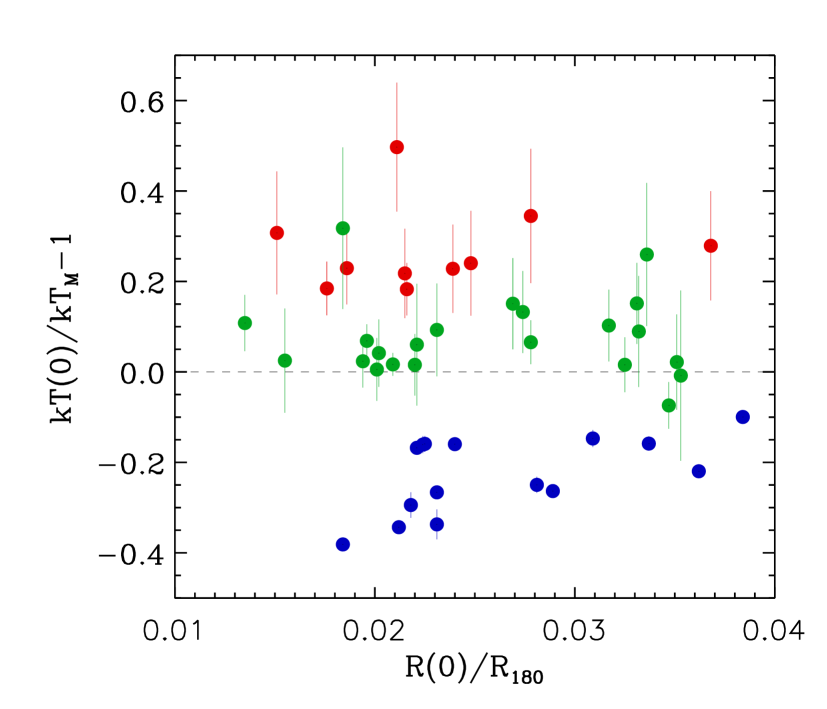
Figure 5: Temperature vs. radius for the innermost ring respectively scaled by $\mathrm{k}T_{\mathrm{M}}$ and $R_{180}$. Clusters for which the temperature is significantly (at least $3\sigma$) lower than $\mathrm{k}T_{\mathrm{M}}$ are defined as cool cores (blue circles); those for which the temperature profile does not significantly (at least $2\sigma$) decrease are defined as non cool cores (red circles); other clusters, whose membership is not clearly determined, are classified as uncertain (green circles). When considering $z>0.2$ clusters, which fill the right-side of the panel, we expect smaller gradients due to the lower spatial resolution.

In Fig. 5 we report temperature and radius of the innermost ring scaled by $\mathrm{k}T_{\mathrm{M}}$ and $R_{180}$ for all clusters. We define cool core (hereafter CC) clusters, those for which the temperature is significantly (at least $3\sigma$) lower than $\mathrm{k}T_{\mathrm{M}}$, non cool core (hereafter NCC) clusters, those for which the temperature profile does not significantly (at least $2\sigma$) decrease, and uncertain (hereafter UNC) clusters, those for which the membership is not clearly determined.

It is worth noting that the error bars are usually strongly asymmetric, i.e. the upper bar is larger than the lower; moreover, the higher the temperature, the larger the error bars. The reason is that most of the information on the temperature is located around the energy of the exponential cut-off; due to the spectral shapes of source and background components and to the sharp decrease of the effective areas at high energies, the source-to-background count rate ratio strongly depends on the energy band (see for example Fig. 3), i.e. the higher the cut-off energy, the lower the source-to-background ratio, the larger the uncertainties.

Figure 6: Mean radial temperature profile rescaled by $R_{180}$ and $\mathrm{k}T_{\mathrm{M}}$. The dotted lines show the one-sigma scatter of the values around the average.

In Fig. 6 we report the weighted average and the scatter of all profiles shown in Fig. 4. The mean profile shows more clearly the decline beyond 0.2 $R_{180}$. The temperature also decreases toward the center because of the presence of cool core clusters.

5 Evaluation of systematic effects

We carefully check our results, searching for possible systematic effects. Prior to the analysis, we make use of extensive simulations to quantify the impact of different spectral components on a simulated temperature profile (“a priori” tests). After the analysis, we investigate how the measured temperature profile changes, when choosing different key parameters (“a posteriori” tests).

5.1 “A priori” tests

We perform simulations that reproduce as closely as possible our analysis procedure. We consider two rings: the external 10^′-12^′, $R_{\mathrm{ext}}$, where we estimate background parameters, and the 4.5^′-6^′, $R_{\mathrm{int}}$, where we measure the temperature. The exposure time for each spectrum is always 20 ks i.e. a representative value for our sample (see Fig. 2). We use the Abell 1689 EPIC-MOS1 observation as a guideline, for producing RMF and ARF, and for choosing typical input parameters. The simulation procedure is structured as follows:

• choice of reasonable input parameters,

• generation of 300 spectra in $R_{\mathrm{ext}}$,

• generation of 500 spectra in $R_{\mathrm{int}}$,

• estimate of background parameters in $R_{\mathrm{ext}}$,

• rescaling background parameters and fitting spectra in $R_{\mathrm{int}}$.

Simulation details are described in each subsection. We test the effect of the cosmic variance (see Sect. 5.1.1), of an inaccurate estimate of the cluster emission in $R_{\mathrm{ext}}$ (see Sect. 5.1.2), and of the QSP component (see Sect. 5.1.3). All results are obtained by fitting spectra in the 0.7-10.0 keV band. We have also conducted a similar analysis for the 2.0-10.0 keV band and have found that the systematics for the two bands are of the same order of magnitude. We recall however that the hard band is characterized by worst statistics, therefore in this case systematic errors are masked by statistical ones and have a smaller impact on the final measurement.

5.1.1 The cosmic variance

We employ a simulation to quantify the effect of the cosmic variance on temperature and normalization measurements. In this simulation we neglect the soft proton contribution; the background components are the HALO, the CXB, and the NXB and they are modeled as for MOS1 in Appendix B. In $R_{\mathrm{ext}}$ there are only background components, while in $R_{\mathrm{int}}$ there is also the thermal source. Normalization input values in $R_{\mathrm{ext}}$ are: $N^{\mathrm{ext}}_{\mathrm{HALO}}=1.6\times 10^{-4}$, $N^{\mathrm{ext}}_{\mathrm{CXB}}=5.0\times 10^{-2}$, and $N^{\mathrm{ext}}_{\mathrm{NXB}}=1.0\times 10^{-2}$; input values in $R_{\mathrm{int}}$ are obtained by rescaling the values in $R_{\mathrm{ext}}$ by the area ratio (i.e. as in Eq. 2 with $K(r)=1.0$). $N_{\mathrm{CXB}}$ is also multiplied by a factor, $F$, that simulates the fluctuation due to the cosmic variance between $R_{\mathrm{int}}$ and $R_{\mathrm{ext}}$; after the excision of brightest point-like sources (see Sect. 3.1.1), 1$\sigma$ fluctuations are expected to be $\approx$ 30%. We then consider 3 cases: a null ($F=1.0$), a positive ($F=1.3$), and a negative ($F=0.7$) fluctuation. Thus, in the first case the input value for CXB in $R_{\mathrm{int}}$ is equal to that rescaled by the area ratio, in the second it is 30% higher, and in the third 30% lower. Input parameters for the thermal model in $R_{\mathrm{int}}$ are: $\mathrm{k}T=6$ keV, $Z=0.2\;Z_{\odot}$, $z=0.2$, and $N_{\mathrm{S}}=7.0\times 10^{-4}$. In $R_{\mathrm{ext}}$, $Z$ and $z$ are fixed to the input values, while $\mathrm{k}T$ and $N_{\mathrm{S}}$ are free. For this particular choice of the parameters, the source-to-background count rate ratio, $I$, is 1.13 (see Sect.4). As explained in Sects. 3.2.1 and 3.2.2, we determine the ranges of variability for $N_{\mathrm{HALO}}$, $N_{\mathrm{CXB}}$, and $N_{\mathrm{NXB}}$ and rescale them in $R_{\mathrm{int}}$; then we fit spectra in the 0.7-10.0 keV band and calculate the weighted averages of $\mathrm{k}T$ and $N_{\mathrm{S}}$ over the 500 simulations.

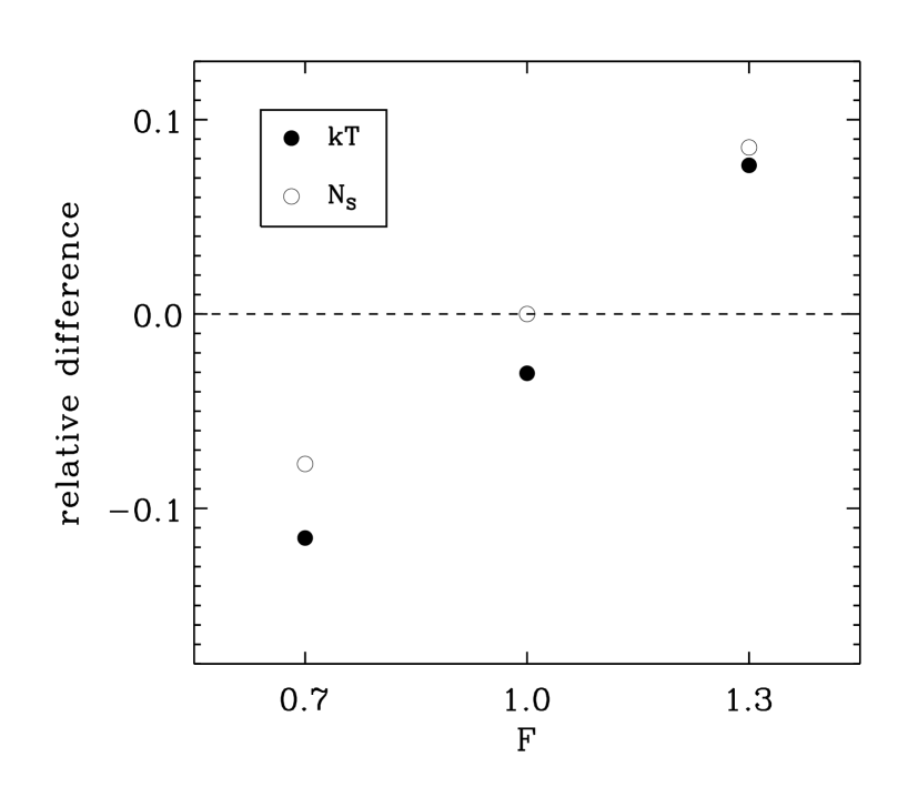
Figure 7: Relative differences between measured and input values for the source temperature, $\mathrm{k}T$, and normalization, $N_{\mathrm{S}}$, as a function of the factor $F$, which simulates the fluctuation due to the cosmic variance (see text for details). Uncertainties are smaller than the circle size. 30% fluctuations cause $\approx$ 10% variations in $\mathrm{k}T$ and $N_{\mathrm{S}}$. For a positive/negative fluctuation the measured $\mathrm{k}T$ and $N_{\mathrm{S}}$ are higher/lower than the input values.

In Fig. 7 we show the relative differences between measured and input values for the temperature, $\mathrm{k}T$ (filled circles), and the normalization, $N_{\mathrm{S}}$ (empty circles). A positive fluctuation of CXB normalization (i.e. $F=1.3$) returns higher temperature and normalization, because the excess of counts due to the CXB is modeled by the thermal component, which is steeper than the CXB power law. For the $F=1.0$ case, while $N_{\mathrm{S}}$ returns exactly the input value, $\mathrm{k}T$ returns a slightly ($\approx$ 3%) underestimated value, probably due to the bias on the temperature estimator (Leccardi & Molendi, 2007). The effect of the cosmic variance is roughly symmetric on both $\mathrm{k}T$ and $N_{\mathrm{S}}$, therefore it is almost negligible when averaging on a large sample. We also perform simulations for our worst case, i.e. $I=0.6$ (see Sect. 4), and find qualitatively the same results: for the $F=1.0$ case, the bias on the temperature is $\approx$ 8% rather than $\approx$ 3% and the bias on the normalization is negligible.

5.1.2 The cluster emission in the 10^′-12^′ ring

The source contribution in the 10^′-12^′ ring, which mainly depends on cluster redshift and emission measure, is difficult to estimate with accuracy. We employ a simulation to determine how an inaccurate estimate could affect our measurement of cluster temperature, $\mathrm{k}T$, and normalization, $N_{\mathrm{S}}$. Soft protons are neglected in this case too; background components and their input values are the same as for the $F=1.0$ case of the cosmic variance tests (see Sect. 5.1.1). Also input parameters for the thermal model in $R_{\mathrm{int}}$ are the same as in that case, instead in $R_{\mathrm{ext}}$ are $\mathrm{k}T^{\mathrm{ext}}=4$ keV, $Z^{\mathrm{ext}}=0.2\;Z_{\odot}$, $z^{\mathrm{ext}}=0.2$, and $N_{\mathrm{S}}^{\mathrm{ext}}=2.5\times 10^{-4}$. For this particular choice of the parameters, the source-to-background count rate ratio, $I$, is 1.13 (see Sect.4). When fitting spectra in $R_{\mathrm{ext}}$, all thermal parameters are fixed: namely the temperature, the metallicity, and the redshift are fixed to the input values, while for $N_{\mathrm{S}}^{\mathrm{ext}}$ we consider 4 cases. In the first case, we neglect the source contribution ($N_{\mathrm{S}}^{\mathrm{ext}}=0$); in the other cases, the normalization is fixed to a value lower ($N_{\mathrm{S}}^{\mathrm{ext}}=1.0\times 10^{-4}$), equal ($N_{\mathrm{S}}^{\mathrm{ext}}=2.5\times 10^{-4}$), and higher ($N_{\mathrm{S}}^{\mathrm{ext}}=4.0\times 10^{-4}$) than the input value. Normalizations of all background components (namely $N_{\mathrm{HALO}}$, $N_{\mathrm{CXB}}$, and $N_{\mathrm{NXB}}$) are free parameters. For each case, we compute the weighted average of $N_{\mathrm{HALO}}$, $N_{\mathrm{CXB}}$, and $N_{\mathrm{NXB}}$ over the 300 spectra in $R_{\mathrm{ext}}$ and compare them to the input values (see Fig. 8).

Figure 8: Relative differences between measured and input values for the normalization of background components (namely $N_{\mathrm{HALO}}$, $N_{\mathrm{CXB}}$, and $N_{\mathrm{NXB}}$) as a function of the input value for cluster normalization in $R_{\mathrm{ext}}$, $N_{\mathrm{S}}^{\mathrm{ext}}$. Uncertainties are smaller than the symbol size. $N_{\mathrm{CXB}}$ shows the strongest (negative) correlation with $N_{\mathrm{S}}^{\mathrm{ext}}$.

$N_{\mathrm{NXB}}$ and $N_{\mathrm{S}}^{\mathrm{ext}}$ are weakly correlated; instead, $N_{\mathrm{HALO}}$ and, in particular, $N_{\mathrm{CXB}}$ show a strong negative correlation with the input value for $N_{\mathrm{S}}^{\mathrm{ext}}$, which depends on their spectral shapes. Note that, if we correctly estimate $N_{\mathrm{S}}^{\mathrm{ext}}$ then $N_{\mathrm{HALO}}$, $N_{\mathrm{CXB}}$, and $N_{\mathrm{NXB}}$ converge to their input values.

Figure 9: Relative differences between measured and input values for the source temperature, $\mathrm{k}T$, and normalization, $N_{\mathrm{S}}$, as a function of the input value for cluster normalization in $R_{\mathrm{ext}}$, $N_{\mathrm{S}}^{\mathrm{ext}}$. Uncertainties are smaller than the symbol size. An underestimate/overestimate of $N_{\mathrm{S}}^{\mathrm{ext}}$ causes $\mathrm{k}T$ and $N_{\mathrm{S}}$ to be underestimated/overestimated.

For each input value of $N_{\mathrm{S}}^{\mathrm{ext}}$ in $R_{\mathrm{ext}}$, we fit spectra in $R_{\mathrm{int}}$ in the 0.7-10.0 keV band after the usual rescaling of background parameters (see Sect. 3.2.2), calculate the weighted averages of the source temperature, $\mathrm{k}T$, and normalization, $N_{\mathrm{S}}$, over the 500 simulations, and compare them to the input values (see Fig. 9). Values of $\mathrm{k}T$ and $N_{\mathrm{S}}$ measured in $R_{\mathrm{int}}$ show a positive correlation with the value of $N_{\mathrm{S}}^{\mathrm{ext}}$ fixed in $R_{\mathrm{ext}}$. This is indeed expected because of the broad similarity in the spectral shapes of thermal and CXB models. In $R_{\mathrm{ext}}$ an overestimate of $N_{\mathrm{S}}^{\mathrm{ext}}$ implies an underestimate of $N_{\mathrm{CXB}}$ (see Fig. 8); $N_{\mathrm{CXB}}$ is then rescaled by the area ratio, thus is underestimated in $R_{\mathrm{int}}$ too; this results in an overestimate of $\mathrm{k}T$ and $N_{\mathrm{S}}$ in $R_{\mathrm{int}}$, as for the $F=1.3$ case of the cosmic variance simulations (see Sect. 5.1.1). Typical uncertainties ($\approx 50\%$) on $N_{\mathrm{S}}^{\mathrm{ext}}$ cause systematic 5% and 7% errors on $\mathrm{k}T$ and $N_{\mathrm{S}}$ (see Fig. 9). Note that, after the correction for the $\approx$ 3% bias mentioned in Sect. 5.1.1, the effect on $N_{\mathrm{S}}$ and $\mathrm{k}T$ is symmetric; thus, when averaging on a large sample, the effect on the mean profile should be almost negligible. Note also that if we were to neglect the cluster emission in the 10^′-12^′ ring ($N_{\mathrm{S}}^{\mathrm{ext}}=0$), we would cause a systematic underestimate of $\mathrm{k}T$ and $N_{\mathrm{S}}$ in the order of 7-10% (see Fig. 9).

In a real case we deal with a combination of fluctuations and cannot treat each one separately, thus we employ a simulation to investigate how fluctuations with different origins combine with each other. We combine effects due to the cosmic variance and to an inaccurate estimate of the cluster emission in the 10^′-12^′ ring, by considering the $F=0.7$, $F=1.0$, and $F=1.3$ cases mentioned in Sect. 5.1.1 and $N_{\mathrm{S}}^{\mathrm{ext}}=1.0\times 10^{-4}$, $N_{\mathrm{S}}^{\mathrm{ext}}=2.5\times 10^{-4}$, and $N_{\mathrm{S}}^{\mathrm{ext}}=4.0\times 10^{-4}$ mentioned in this section. The simulation procedure is the same as described before. For the cluster normalization, we find that fluctuations combine in a linear way and that effects are highly symmetric with respect to the zero case ($F=1.0$ for the cosmic variance and $N_{\mathrm{S}}^{\mathrm{ext}}=2.5\times 10^{-4}$ for the cluster emission in the 10^′-12^′ ring). For the cluster temperature, we find again the $\approx$ 3% bias related to the estimator; once accounted for this 3% offset, results are roughly similar to those found for the normalization case. To be more quantitative, when averaging on a large sample, the expected systematic on the temperature measurement is $\approx$ 3% due to the biased estimator and $\lesssim$ 2% due to deviations from the linear regime.

5.1.3 The QSP component

A careful characterization of the QSP component is crucial for our data analysis procedure. We employ a simulation to quantify how an incorrect estimate of the QSP contribution from the “IN over OUT” diagnostic, i.e. the $R_{\mathrm{SB}}=1.10$ (see Sect. 3.1.2) could affect our measurements. The spectral components and their input values are the same as for the $F=1.0$ case of the cosmic variance simulations (see Sect. 5.1.1), plus the QSP component in both rings. The model for QSP is the same as described in Appendix B. We choose two input values for $N_{\mathrm{QSP}}$ corresponding to a standard ($R_{\mathrm{SB}}=1.10$) and a high ($R_{\mathrm{SB}}=1.40$) level of QSP contamination. For these particular choices of the parameters, the source-to-background count rate ratio, $I$, is 1.06 for $R_{\mathrm{SB}}=1.10$ and 0.77 for $R_{\mathrm{SB}}=1.40$ (see Sect.4). For each input value we consider 2 cases: an underestimate ($R_{\mathrm{SB}}=1.05-1.35$) and an overestimate ($R_{\mathrm{SB}}=1.15-1.45$) of the correct value. By fitting spectra in $R_{\mathrm{ext}}$ in the 0.7-10.0 keV band, we determine the range of variability of $N_{\mathrm{HALO}}$, $N_{\mathrm{CXB}}$, and $N_{\mathrm{NXB}}$ and rescale it in $R_{\mathrm{int}}$ (see Sect. 3.2.2).

Figure 10: Relative differences between measured and input values for the source temperature, $\mathrm{k}T$, and normalization, $N_{\mathrm{S}}$, as a function of the input value for the QSP contribution, $R_{\mathrm{SB}}$. Uncertainties are smaller than the circle size. Upper panel: $R_{\mathrm{SB}}$ is underestimated to 1.05 and 1.35 with respect to 1.10 and 1.40. Lower panel: $R_{\mathrm{SB}}$ is overestimated to 1.15 and 1.45. See text for the discussion.

We then fit spectra in $R_{\mathrm{int}}$ and compare the weighted averages of cluster temperature, $\mathrm{k}T$, and normalization, $N_{\mathrm{S}}$, to their input values (see Fig. 10).

When considering $N_{\mathrm{S}}$, the relative difference between measured and input values is $<5\%$ for all cases and the effect is symmetric, therefore the impact on the mean profile obtained from a large sample should be very small. On the contrary, $\mathrm{k}T$ strongly depends on our estimate of the QSP component: the relative difference is $\approx$ 5% for $R_{\mathrm{SB}}=1.10$ and $\approx$ 20% for $R_{\mathrm{SB}}=1.40$. When overestimating $R_{\mathrm{SB}}$, $\mathrm{k}T$ is underestimated, because of the broad similarity in the spectral shapes of the two components. In the $R_{\mathrm{SB}}=1.40$ case, the values corresponding to an overestimate and an underestimate, although symmetric with respect to zero, are characterized by different uncertainties (errors in the first case are twice than in the second); thus, a weighted average returns a 10% underestimated value.

5.2 “A posteriori” tests

In this subsection we investigate how the mean profile is affected by a particular choice of key parameters, namely: the last ring for which we measure a temperature (see Sect. 5.2.1), the energy band used for the spectral fitting (see Sect. 5.2.2), and the QSP contamination (see Sect. 5.2.3).

5.2.1 The truncation radius

In Sect. 4 we have introduced the indicator $I$ to choose the last ring where our temperature measurement is reliable. Here we produce mean temperature profiles by averaging all measurements for which $I>I_{0}$, for different values of the threshold $I_{0}$.

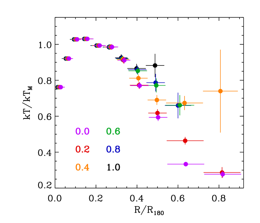
Figure 11: Mean temperature profiles computed by choosing different values for the threshold $I_{0}$ (defined in Sect. 4) plotted with different colors. There is a clear systematic effect: the smaller the threshold, the steeper the profile. The radii have been slightly offset in the plot for clarity.

In Fig. 11 we report the profiles obtained in the 0.7-10.0 keV band for different choices of $I_{0}$ (namely 0.0, 0.2, 0.4, 0.6, 0.8, and 1.0). As expected, the smaller is the threshold, the further the mean profile extends. If we focus on the points between 0.3 and 0.6 of $R_{180}$, we notice a clear systematic effect: the smaller the threshold, the lower the temperature. This means that, on average, the temperature is lower in those rings where the background is more important. This systematic effect becomes evident where cluster emission and background fluctuations are comparable and is probably related to small imperfections in our background modeling and to the bias on the temperature estimator (see Sect. 5.1.1). The imperfections of our background model becomes the dominant effect for small values of $I$ (namely $I\lesssim 0.4$). Thus, under a certain threshold, $I_{0}$, our measurements are no longer reliable. Fig. 11 shows that $I_{0}=0.6$ represents a good compromise. Indeed, when considering the region between 0.4 and 0.5 of $R_{180}$ and comparing the average value for $\mathrm{k}T$ obtained for a threshold $I_{0}=0.6$ and for $I_{0}=1.0$, we find a small ($4\%\pm 3\%$) relative difference.

5.2.2 Fitting in different bands

We have fitted spectra in two different energy bands (i.e. 0.7-10.0 keV and 2.0-10.0 keV), each one characterized by different advantages and drawbacks (see Sect. 3.2). The indicator, $I$, defined in Sect. 4 depends on the band in which the count rate is calculated: more precisely, $I$(0.7-10.0) is roughly 1.5 times greater than $I$(2.0-10.0) for small values (i.e. $I\lesssim 2.0$). The threshold $I_{0}=0.6$ in the 0.7-10.0 keV band corresponds to $I_{0}=0.4$ in the 2.0-10.0 keV band (see Sect. 5.2.1).

Figure 12: Mean temperature profiles obtained by fitting spectra in the 0.7-10.0 keV (filled circles) and in the 2.0-10.0 keV band (empty circles). The profiles are very similar, except for the innermost point. The radii have been slightly offset in the plot for clarity.

In Fig. 12 we compare the mean temperature profile obtained in the 0.7-10.0 keV band ($I_{0}=0.6$) with that obtained in the 2.0-10.0 keV band ($I_{0}=0.4$). The profiles are very similar, except for the innermost point. The uncertainties in the 0.7-10.0 case are much smaller at all radii, even if the total number of points (i.e. the number of rings for all cluster) is the same; this is because the higher statistics at low energies allows to substantially reduce the errors on single measurements.

In the most internal point a high discrepancy between the two measurements is present, although in that region the background is negligible. This is due to the superposition, along the line of sight, of photons emitted by optically thin ICM with different density and temperature. When looking at the center of cool core clusters, the line of sight intercepts regions characterized by strong temperature gradients, therefore the accumulated spectrum is the sum of many components at different temperatures. In this case, the best fit value for the temperature strongly depends on the energy band (i.e. the harder the band, the higher the temperature), because the exclusion of the soft band implies the exclusion of most of the emission from cooler components (Mazzotta et al., 2004).

5.2.3 Contamination from QSP

We divide clusters in our sample in four groups, according to the QSP contamination that we estimate from $R_{\mathrm{SB}}$ (see Sect. 3.1.2).

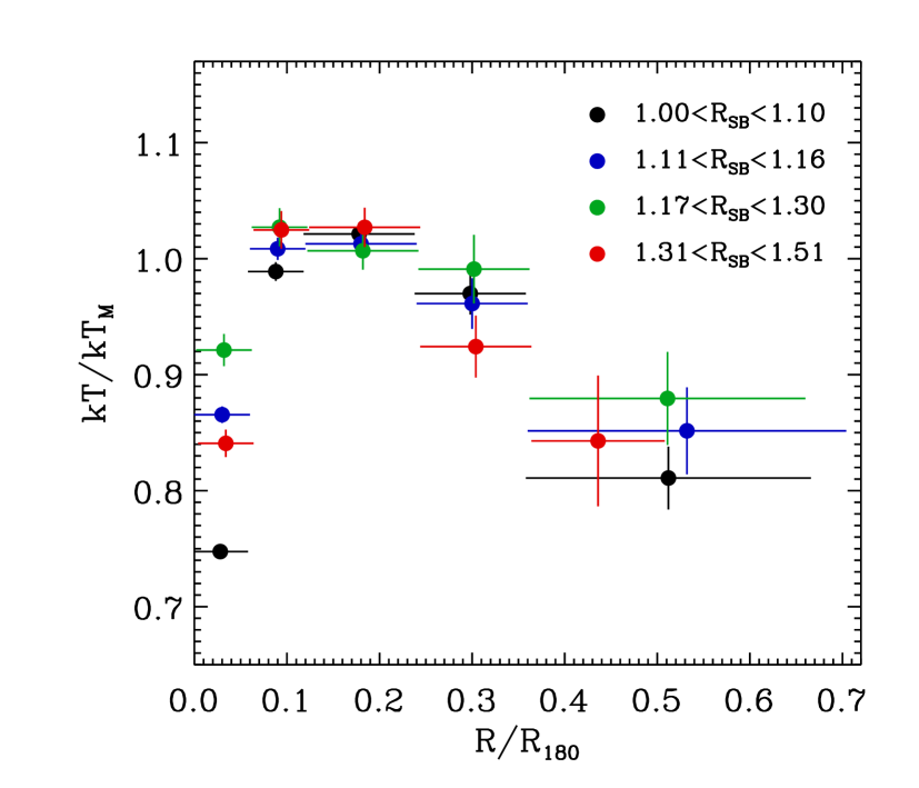
Figure 13: Mean temperature profiles as a function of the QSP contamination, $R_{\mathrm{SB}}$. The four profiles are fully consistent, no correlation is found between the shape of the profiles and $R_{\mathrm{SB}}$. The radii have been slightly offset in the plot for clarity.

In Fig. 13 we report the mean temperature profiles for the four groups, by fitting spectra in the 0.7-10.0 keV band and fixing $I_{0}=0.6$. When dividing clusters in subsamples, we choose larger bin sizes to reduce the error bars. When $R_{\mathrm{SB}}$ is high, our selection criterion based on the source-to-background count rate ratio (see Sects. 4 and 5.2.1) excludes the outer rings, indeed the red profile extends out to only 0.5 $R_{180}$. The four profiles are fully consistent, no correlation is found between the shape of the profiles and $R_{\mathrm{SB}}$. The discrepancy in the innermost ring is due to the presence of a different number of cool core clusters in each group. We therefore conclude that the systematic error associated to the QSP contamination is smaller than statistical errors ($\approx$ 7% beyond 0.4 $R_{180}$).

5.3 A budget for systematics

In this subsection we summarize the main results for what concern systematic errors associated to our mean profile. We compare expected systematics computed from “a priori” tests with measured systematics from “a posteriori” tests.

The $F=1.0$ case in Sect. 5.1.1 and the $N_{\mathrm{S}}^{\mathrm{ext}}=2.5\times 10^{-4}$ case in Sect. 5.1.2 show that our analysis procedure is affected by a 3% to 8% systematic underestimate of the temperature, when analyzing the outermost rings; the bias is probably related to the temperature estimator as described in Leccardi & Molendi (2007). On the contrary the normalization estimator is unbiased. In Sects. 5.1.1 and 5.1.2 we also found that the effects of the cosmic variance and of an inaccurate estimate of the cluster emission in the external ring are symmetric for both the temperature, $\mathrm{k}T$, and the normalization, $N_{\mathrm{S}}$. In Sect. 5.1.2 we found that the effects due to fluctuations with different origins combine in a linear way and, when averaging on a large sample, the systematic associated to the mean profile is almost negligible for $N_{\mathrm{S}}$ and $\lesssim$ 2% for $\mathrm{k}T$. Thus, the expected systematic for $\mathrm{k}T$ is $\lesssim$ 5%.

In Sect. 5.1.3 we found that, for a standard level of contamination ($R_{\mathrm{SB}}=1.10$), a typical 5% error in the estimate of $R_{\mathrm{SB}}$ causes negligible effects on both measurements of cluster temperature and normalization. The same error causes negligible effects on $N_{\mathrm{S}}$ measurements also for a high level of contamination ($R_{\mathrm{SB}}=1.40$). On the contrary, effects on $\mathrm{k}T$ for $R_{\mathrm{SB}}=1.40$ are important: the same 5% error causes a 10% underestimate of $\mathrm{k}T$, also when averaging on a large sample. However, at the end of Sect. 5.2.3 in particular from Fig. 13, we have concluded that, when considering the whole sample, the systematic error associated to the QSP contamination is smaller than statistical errors ($\approx$ 7% beyond 0.4 $R_{180}$). The difference between expected and measured systematic errors is only apparent. Indeed, when analyzing our sample, we average measurements that span a wide range of values for $R_{\mathrm{SB}}$ and $I$; conversely, the 10% systematic error is expected for an unfavorable case, i.e. $R_{\mathrm{SB}}=1.40$ and $I=0.77$ (see Sect. 5.1.3).

In Sect. 5.2.1 we compared the mean temperature value obtained for a threshold $I_{0}=0.6$ and for $I_{0}=1.0$ in an outer region (i.e. between 0.4 and 0.5 of $R_{180}$). In this ring the mean value for the indicator $I$ is 1.14, thus the expected bias related to the temperature estimator is $\approx$ 3% (see Sect. 5.1.1). We measured a $4\%\pm 3\%$ temperature discrepancy, which is consistent with the expected bias. As pointed out in Sect. 5.2.1, the discrepancy could also be due to small imperfections in our background model; we are not able to quantify the amount of this contribution, but we expect it to be small when considering $I>0.6$.

To summarize, in external regions our measurements of the cluster temperature are affected by systematic effects, which depends on the radius through the factor $I$, i.e. the source-to-background count rate ratio. For each ring, we calculate the mean value for $I$, estimate the expected bias from simulations, and apply a correction to our mean profile. The expected bias is negligible for internal rings out to 0.30 $R_{180}$ (for which $I\gtrsim 3$), is 2-3% for 0.30-0.36 and 0.36-0.45 bins, and is $\approx 5\%$ for the last two bins (i.e. 0.45-0.54 and 0.54-0.70). We associate to our correction an uncertainty of the same order of the correction itself, accounting for our limited knowledge from our “a posteriori” tests of the precise value of the bias.

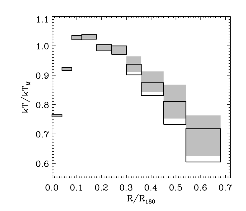
Figure 14: Mean temperature profile rescaled by $R_{180}$ and $\mathrm{k}T_{\mathrm{M}}$. For each ring, empty boxes and shaded regions indicate one sigma uncertainties respectively before and after the bias correction.

Table 4: Mean temperature values rescaled by $\mathrm{k}T_{\mathrm{M}}$ and corrected for the biases discussed in the text, for each interval in units of $R_{180}$.

Ringa	Temperatureb
0.00-0.04	0.762$\pm$0.004
0.04-0.08	0.921$\pm$0.005
0.08-0.12	1.028$\pm$0.007
0.12-0.18	1.030$\pm$0.008
0.18-0.24	0.993$\pm$0.010
0.24-0.30	0.985$\pm$0.014
0.30-0.36	0.938$\pm$0.026
0.36-0.45	0.878$\pm$0.035
0.45-0.54	0.810$\pm$0.058
0.54-0.70	0.694$\pm$0.069

• ^a in units of $R_{180}$; ^b in units of $\mathrm{k}T_{\mathrm{M}}$.

In Fig. 14 we show the mean temperature profile before and after the correction for the bias. In Table 4 we report for each bin the corrected values; the uncertainty is the quadrature sum of the statistical error and of the error associated to our correction. Hereafter, we will consider the mean profile corrected for the bias, unless otherwise stated. Note that the bias is always comparable with the statistical uncertainties. For this reason, ours can be considered as a definitive work, for what concerns the measurement of radial temperature profiles of galaxy clusters with XMM-Newton. We have reached the limits imposed by the instrument and by the analysis technique, so that further increasing of the number of objects will not improve the quality of the measurement.

6 The mean temperature profile

6.1 Characterizing the profile

We fit profiles (see Fig. 4) beyond 0.2 $R_{180}$ with a linear model and a power law to characterize the profile decline. By using a linear model

$$\frac{\mathrm{k}T}{\mathrm{k}T_{\mathrm{M}}}=\mathrm{A}-\mathrm{B}\left(\frac{R}{R_{180}}-0.2\right)$$ (4)

we find $\mathrm{A}=1.02\pm 0.01$ and $\mathrm{B}=0.77\pm 0.11$; by using a power law

$$\frac{\mathrm{k}T}{\mathrm{k}T_{\mathrm{M}}}=\mathrm{N}\left(\frac{R}{0.2\;R_{180}}\right)^{-\mu}$$ (5)

we find $\mathrm{N}=1.03\pm 0.01$ and $\mu=0.24\pm 0.04$. If the gas can be approximated by a polytrope, we can derive its index, $\gamma$, from the slope of projected temperature profiles, $\mu$ (De Grandi & Molendi, 2002):

$$\gamma=1+\mu/2,$$ (6)

under the assumption that, at large radii, three-dimensional gas temperature and density profiles be well described, respectively, by a power law and a $\beta$-model with $\beta=2/3$. For $R>0.2\;R_{180}$, we measure $\gamma=1.12\pm 0.02$, which is an intermediate value between those associated to isothermal ($\gamma=1.0$) and adiabatic ($\gamma=1.67$) gas.

Figure 15: Power-law best-fit parameters obtained by fitting profiles beyond a variable radius, $R_{\mathrm{min}}$, in units of $R_{180}$. The normalization is calculated at 0.2. The index best-fit value is not constant with $R_{\mathrm{min}}$, thus the ICM cannot be considered as a polytrope.

However, we note that the power-law best-fit parameters depend on the chosen region (see Fig. 15), as well as the derived $\gamma$, thus the above values should be taken with some caution.

6.2 Redshift evolution

We divide our clusters in four groups according to the redshift, to investigate a possible evolution of temperature profiles with cosmic time.

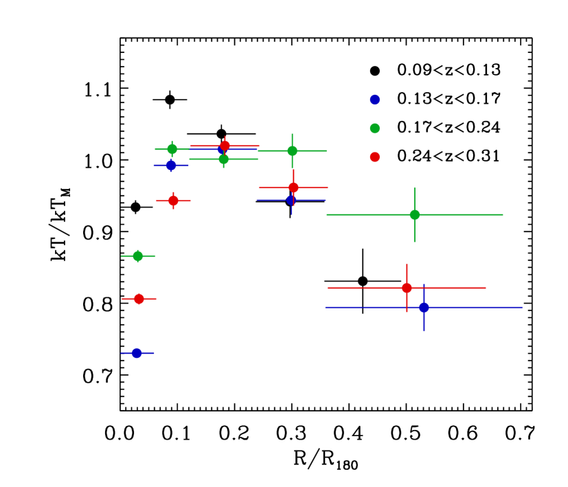
Figure 16: Mean temperature profiles for the four $z$-binned groups of clusters. There is no indication of profile evolution. The radii have been slightly offset in the plot for clarity.

In Fig. 16 we report the mean temperature profiles for the four groups. Spectra are fitted in the 0.7-10.0 keV band and $I_{0}=0.6$ (see Sect. 4). As in the following Sects. 6.3 and 6.4, when dividing clusters in subsamples, the profiles are not corrected for biases (see Sect. 5.3), because when comparing subsamples we are not interested in determining the absolute value of the temperature, but in searching for relative differences. Moreover, in Fig. 16 and in Fig. 18 we choose larger bin sizes to reduce the error bars (as in Fig. 10). The four profiles are very similar: the discrepancy in the outer regions is comparable to statistical and systematic errors, the difference in the central region is due to a different fraction of cool core clusters.

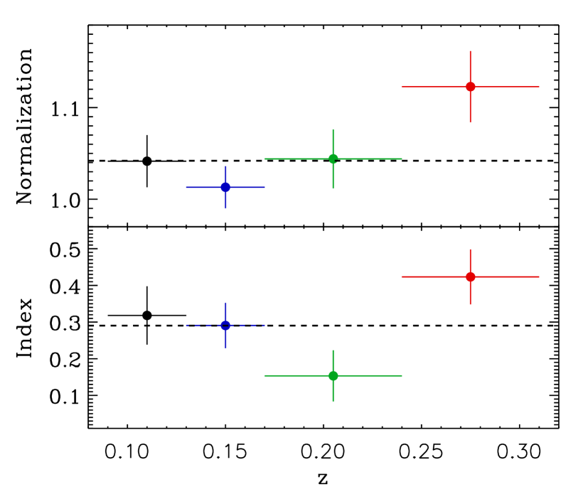
Figure 17: Best fit parameters obtained by fitting each group of profiles with a power law beyond 0.2 $R_{180}$. The normalization is calculated at 0.2 $R_{180}$. The dashed lines indicate the best fit values for the whole sample. No clear correlation is found between power-law parameters and the redshift.

We fit each group of profiles with a power law beyond 0.2 $R_{180}$ and report results in Fig. 17. Since there is no clear correlation between the two parameters and the redshift, we conclude that from the analysis of our sample there is no indication of profile evolution up to $z=0.3$.

6.3 Cool core and non cool core clusters

In Sect. 4 we defined three groups: clusters that clearly host a cool core, clusters with no evidence of a cool core, and uncertain clusters.

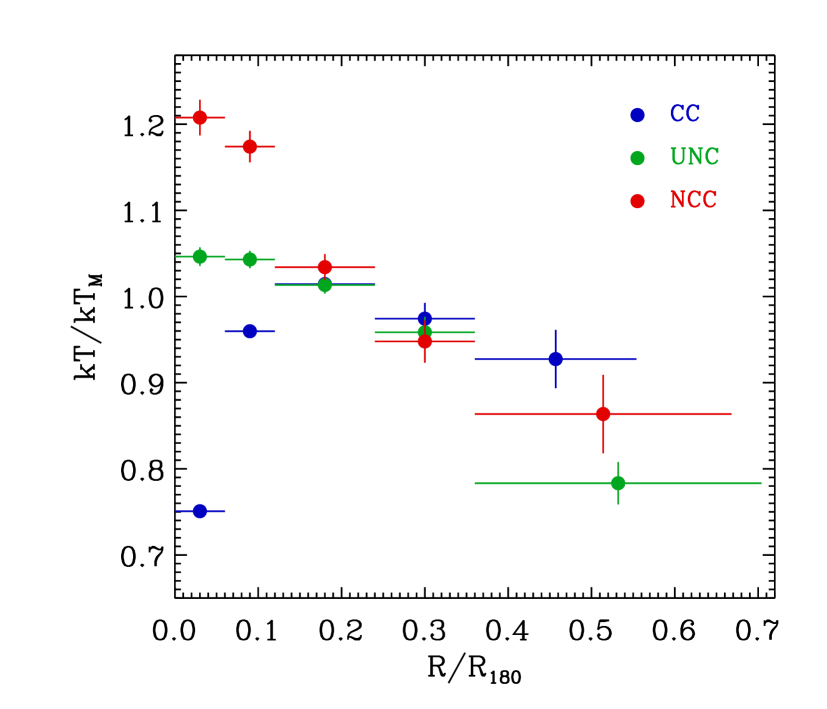
Figure 18: Mean temperature profiles for cool core (blue), non cool core (red), and uncertain (green) clusters. Profiles differ by definition in the core region and are consistent in the outer regions.

In Fig. 18 we show mean temperature profiles for the three groups. Spectra are fitted in the 0.7-10.0 keV band and $I_{0}=0.6$. Profiles differ by definition in the core region and are consistent beyond $\approx$ 0.1 $R_{180}$.

6.4 REFL04 and LP07 subsamples

Our sample is not complete with respect to any property. However, most of our clusters ($\approx 2/3$) belong to the REFLEX Cluster Survey catalog (Böhringer et al., 2004), a statistically complete X-ray flux-limited sample of 447 galaxy clusters, and a dozen objects belong to the XMM-Newton Legacy Project sample (Pratt et al., 2007), which is representative of an X-ray flux-limited sample with $z<0.2$ and $\mathrm{k}T>2$ keV. We then select two subsamples from our sample: clusters that belong to the REFLEX catalog (REFL04 subsample) and to the Legacy Project sample (LP07 subsample). The smaller (i.e. the LP07) is derived from Pratt’s parent sample, by applying our selection criteria based on cluster temperature and redshift. We also exclude cluster observations that are heavily affected by soft proton contamination, however the latter selection should be equivalent to a random choice and introduce no bias. Thus, we expect the LP07 subsample to be representative of an X-ray flux-limited sample of galaxy clusters with $0.1<z<0.2$ and $\mathrm{k}T>3.3$ keV. The larger (i.e. the REFL04) subsample includes the LP07 one. Clusters that belong to the REFL04, but not to the LP07, were observed with XMM-Newton for different reasons, they are not part of a large program and almost all observations have different PIs. Thus, there are no obvious reasons to believe that the sample is significantly biased with respect to any fundamental cluster property. A similar reasoning leads to the same conclusion for our whole sample.

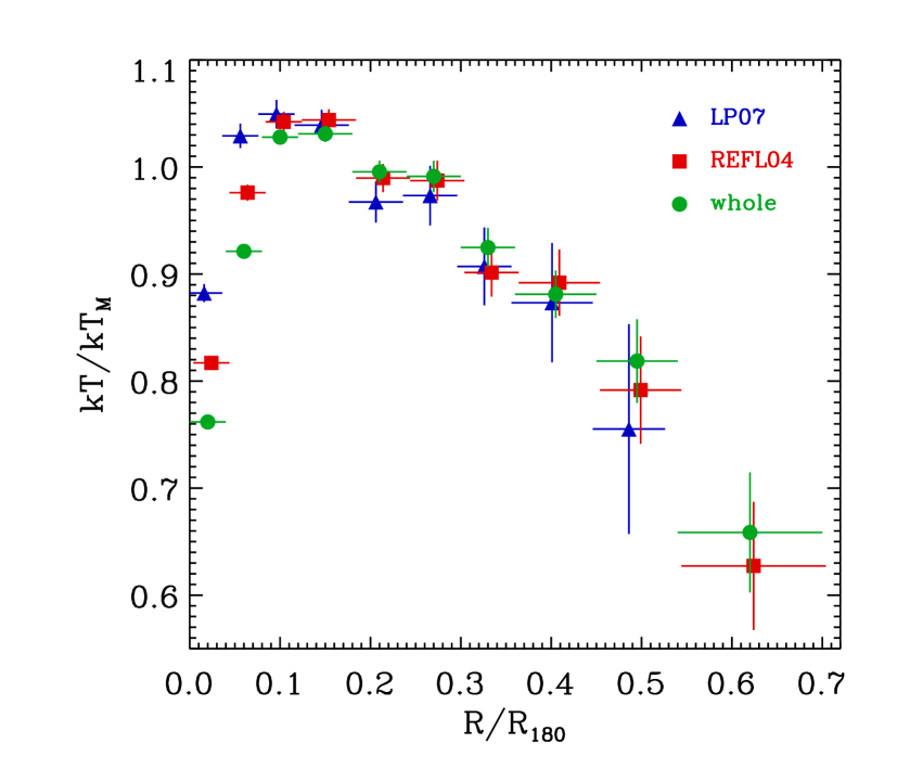
Figure 19: Mean temperature profiles obtained from the LP07 subsample (blue triangles), the REFL04 subsample (red squares) and the whole sample (green circles). The three profiles are fully consistent in the outer regions. The radii have been slightly offset in the plot for clarity.

In Fig. 19 we compare mean temperature profiles obtained from the two subsamples and the whole sample. The three profiles are fully consistent beyond $\approx$ 0.1 $R_{180}$, the difference in the central region is due to a different fraction of CC clusters. These results allow us to conclude that our whole sample is representative of hot, intermediate redshift clusters with respect to temperature profiles, i.e. the quantity we are interested in.

6.5 Comparison with hydrodynamic simulations

In this subsection we compare our mean temperature profile with that derived from cluster hydrodynamic simulations by Borgani et al. (2004) (hereafter B04). The authors used the TREE+SPH code GADGET (Springel et al., 2001) to simulate a concordance cold dark matter cosmological model ($\Omega_{\mathrm{m}}=0.3$, $\Omega_{\Lambda}=0.7$, $\sigma_{8}=0.8$, and $h=0.7$) within a box of 192 $h^{-1}$ Mpc on a side, 480³ dark matter particles and as many gas particles. The simulation includes radiative cooling, star formation and supernova feedback. Simulated cluster profiles are scaled by the emission weighted global temperature and $R_{180}$ calculated from its definition (i.e. the radius encompassing a spherical density contrast of 180 with respect to the critical density).

Figure 20: Comparison between our observed mean profile (circles) and that derived from hydrodynamic simulations (Borgani et al., 2004) by averaging over clusters with $\mathrm{k}T>3$ keV (solid line). The dashed line is obtained by rescaling the solid one by 10%.

In Fig. 20 we compare our observed profile to the projected mean profile obtained by averaging over simulated clusters with $\mathrm{k}T>3$ keV. The evident mismatch between the two profiles is most likely due to a different definition for the scaling temperature: actually it is known that the emission weighted temperature is higher than the mean temperature obtained from observational data (Mazzotta et al., 2004). By rescaling the B04 profile by 10%, we find a good agreement between simulation and our data beyond $\approx$ 0.25 $R_{180}$. Conversely in the core region, simulations are not able to reproduce the observed profile shape.

6.6 Comparison with previous observations

In this subsection we compare our mean temperature profile (LM08) with those obtained by other authors, namely De Grandi & Molendi (2002), Vikhlinin et al. (2005), and Pratt et al. (2007). De Grandi & Molendi (DM02) have analyzed a sample of 21 hot ($\mathrm{k}T>3.3$ keV), nearby ($z\lesssim 0.1$) galaxy clusters observed with BeppoSAX. Their sample includes both CC and NCC clusters. Vikhlinin et al. (V05) have analyzed a sample of 13 nearby ($z\lesssim 0.2$), relaxed galaxy clusters and groups observed with Chandra. We select from their sample only the hottest ($\mathrm{k}T>3.3$ keV) 8 clusters, for a more appropriate comparison with our sample. Pratt et al. (P07) have analyzed a sample of 15 hot ($\mathrm{k}T>2.8$ keV), nearby ($z\lesssim 0.2$) clusters observed with XMM-Newton. Clusters of their sample present a variety of X-ray morphology.

Comparing different works is not trivial. Cluster physical properties, instrumental characteristics, and data analysis procedures may differ. Moreover, each author uses his own recipe to calculate a mean temperature and to derive a scale radius. We have rescaled temperature profiles obtained by other authors, by using the standard cosmology (see Sect. 1) and calculating the mean temperature, $\mathrm{k}T_{\mathrm{M}}$, and the scale radius, $R_{180}$, as explained in Sect. 4; the aim is to reduce as much as possible all inhomogeneities.

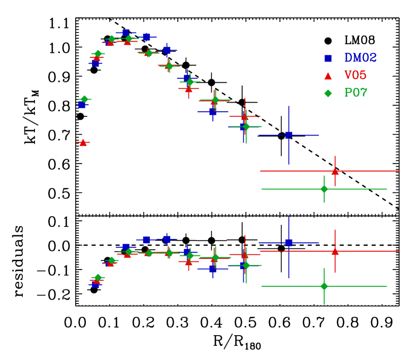
Figure 21: Upper panel: mean temperature profiles obtained from this work (black circles, LM08), by De Grandi & Molendi (blue squares, DM02), by Vikhlinin et al. (red upward triangles, V05), and by Pratt et al. (green diamonds, P07). All profiles are rescaled by $\mathrm{k}T_{\mathrm{M}}$ and $R_{180}$ as defined in Sect. 4. The dashed line shows the best fit with a linear model beyond 0.2 $R_{180}$ (see Sect. 6.1) and is drawn to guide the eye. Lower panel: residuals with respect to the linear model. The LM08 profile is the flattest one.

In Fig. 21 we compare the four mean temperature profiles, rescaled by $\mathrm{k}T_{\mathrm{M}}$ and $R_{180}$. Due to the correction for the biases described in Sect. 5.3, our mean profile is somewhat flatter than others beyond $\approx$ 0.2 $R_{180}$. Discrepancies in the core region are due to a different fraction of CC clusters. The outermost point of the P07 profile is $\approx$ 25% lower, however it is constrained only by two measurements beyond $\approx$ 0.6 $R_{180}$. Our indicator, $I$, (see Sect. 4) warns about the reliability of these two measurements, for which $I\approx$ 0.3, i.e. a half of our threshold, $I_{0}=0.6$. In Fig. 11 we showed that, when using our analysis technique, lower values of $I$ are associated to a bias on the temperature measurement. We assume that a somewhat similar systematic may affect the P07 analysis technique too. When excluding these two measurements, the P07 mean profile only extends out to $\approx$ 0.6 $R_{180}$ and is consistent with ours (see also Fig. 22). It is possible that also measurements obtained with other experiments be affected by a similar kind of systematics, which make the profiles steeper.

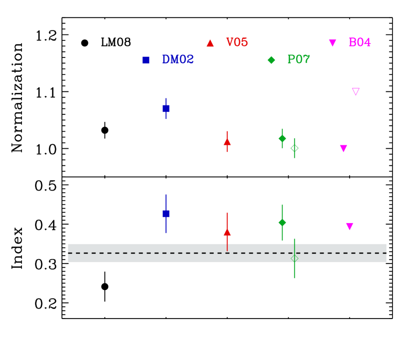
Figure 22: Best fit parameters, obtained by fitting with a power law observed and simulated cluster profiles, beyond 0.2 $R_{180}$: in the upper panel we report the normalization, in the lower the index. We use the same symbols as in Fig. 21 for observed clusters and a violet downward triangle for Borgani’s work (B04). The normalization is calculated at 0.2 $R_{180}$. For P07 we report two values, empty diamonds indicate index and normalization obtained when excluding the two outermost measurements (see text for details). The empty downward triangle indicates the normalization of the B04 rescaled profile (see Sect. 6.5). In the lower panel, the dashed line and the shaded region represent the weighted average and its one sigma confidence interval derived from the observed profiles only (for P07 we use the lower value, i.e. the empty diamond). As previously noted from Fig. 21, the LM08 profile is the flattest one, but all indices of observed profiles are consistent within two sigma. Conversely, the B04 profile seems to be significantly steeper, but in this case we are not able to provide an estimate of parameter uncertainty.

We fit observed and simulated cluster profiles with a power law beyond 0.2 $R_{180}$ and in Fig. 22 report best fit parameters. The LM08 profile is the flattest one, however all observed profile indices are consistent within 2-3 sigma. In Sect. 5.3 we have quantified the systematic underestimate on the temperature measurement associated to our procedure. Since it depends on the indicator $I$, which itself depends on the radius, we expect a net effect also on the profile index, $\mu$, namely we expect $\mu$ to be overestimated. For this reason, it is possible that the discrepancy between indices obtained from different works (reported in Fig. 22) may not have a purely statistical origin. We calculate an average profile index, $\mu=0.31\pm 0.02$, which is significantly lower than that obtained from the B04 profile, $\mu=0.39$; however, for the simulation we are not able to provide an estimate of parameter uncertainty.

7 Summary and conclusions

We have analyzed a sample of $\approx 50$ hot, intermediate redshift galaxy clusters (see Sect. 2) to measure their radial properties. In this paper we focused on the temperature profiles and postpone the analysis of the metallicity to a forthcoming paper (Leccardi & Molendi 2008, in preparation). In Sect. 6.4 we showed that our sample should be representative of hot, intermediate redshift clusters, at least with respect to the temperature profile.

Our main results are summarized as follows:

• the mean temperature profile declines with radius in the 0.2 $R_{180}$-0.6 $R_{180}$ range (see Sect. 4);

• when excluding the core region, the profiles are characterized by an intrinsic dispersion (6%) comparable to the estimated systematics, (see Sect. 4);

• there is no evidence of profile evolution with redshift out to $z\approx 0.3$ (see Sect. 6.2);

• the profile slope in the outer regions is independent of the presence of a cool core (see Sect. 6.3);

• the slope of our mean profile is broadly similar to that obtained from hydrodynamic simulations, we find a discrepancy of $\approx 10\%$ in normalization probably due to a different definition for the scaling temperature (see Sect. 6.5);

• when compared to previous works, our profile is somewhat flatter (see Sect. 6.5), probably due to a different level of characterization of systematic effects, which become very important in the outer regions.

The above results have been obtained using a novel data analysis technique, which includes two major improvements. Firstly, we used the background modeling, rather than the background subtraction, and the Cash statistic rather than the $\chi^{2}$; this method requires a careful characterization of all background components. Secondly, we assessed in details systematic effects. We performed two groups of test: prior to the analysis, we made use of extensive simulations to quantify the impact of different components on simulated spectra; after the analysis, we investigated how the measured temperature profile changes, when choosing different key parameters.

From a more general point of view, ours is an attempt to measure cluster properties, as far out as possible, with EPIC instruments. Perhaps, the most important justification for our efforts in this direction is that, for the next 5-10 years, there will be no experiments with comparable or improved capabilities, as far as low surface brightness emission is concerned.

Appendix A The analysis of “closed” observations

We have analyzed a large number ($\approx$ 50) of observations with the filter wheel in the “closed” position to characterize in detail the EPIC-MOS internal background and to provide constraints to the background model, which we use for analyzing our data. Exposure times of individual observations span between 5 and 100 ks for a total exposure time of $\approx$ 650 ks.

For each observation, we select 6 concentric rings (0^′-2.75^′, 2.75^′-4.5^′, 4.5^′-6^′, 6^′-8^′, 8^′-10^′, and 10^′-12^′) centered on the detector center. For each instrument (i.e. MOS1 and MOS2) and each ring, we produce the total spectrum by summing, channel by channel, spectral counts accumulated during all observations. The appropriate RMF is associated to each total spectrum and a minimal grouping is performed to avoid channels with no counts. In Fig. 23 we report the total spectra accumulated in the 10^′-12^′ ring, for MOS1 and MOS2, in the 0.2-11.3 keV band.

Figure 23: MOS1 (thick) and MOS2 (thin) spectra from closed observations in the whole energy band, i.e. 0.2-11.3 keV. MOS2 spectrum is scaled by a factor of 2 for clarity. Spectra are accumulated in the 10^′-12^′ ring. The total exposure time is $\approx$ 650 ks.

Closed observation events are solely due to the internal background, which is characterized by a cosmic-ray induced continuum (NXB) plus several fluorescence emission lines. The most intense lines are due to Al ($\approx$ 1.5 keV) and Si ($\approx$ 1.8 keV). Beyond 2 keV we fit the NXB with a single power law (index 0.24 and 0.23 for MOS1 and MOS2 respectively); instead, for the 0.7-10.0 keV range, a broken power-law (see Table 5) is more appropriate. Emission lines are modeled by Gaussians. Note that particle background components are not multiplied by the effective area.

Table 5: Best fit parameters for the NXB broken power law. $\Gamma_{1}$ and $\Gamma_{2}$ are the slopes below and above the break energy, $E_{\mathrm{B}}$.

	$\Gamma_{1}$	$E_{\mathrm{B}}$ [keV]	$\Gamma_{2}$
MOS1	0.22	7.0	0.05
MOS2	0.32	3.0	0.22

In Table 6 we list the emission lines of our model with their rest frame energies.

Table 6: Instrumental emission lines in the 0.7-10.0 keV energy band.

Line	E [keV]	Line	E [keV]
Al K$\alpha$	1.487	Mn K$\beta$	6.490
Al K$\beta$	1.557	Fe K$\beta$	7.058
Si K$\alpha$	1.740	Ni K$\alpha$	7.472
Si K$\beta$	1.836	Cu K$\alpha$	8.041
Au M$\alpha$	2.110	Ni K$\beta$	8.265
Au M$\beta$	2.200	Zn K$\alpha$	8.631
Cr K$\alpha$	5.412	Cu K$\beta$	8.905
Mn K$\alpha$	5.895	Zn K$\beta$	9.572
Cr K$\beta$	5.947	Au L$\alpha$	9.685
Fe K$\alpha$	6.400

Normalization values are always reported in XSPEC units. Lines are determined by 3 parameters: peak energy, intrinsic width and normalization. The energy of Al K$\alpha$, E_Al, is free to allow for a small shift in the energy scale; the energies of Al, Si, and Au-M lines are linked to E_Al in such a way that a common shift, $\Delta$E, is applied to all lines. Similarly, the energy of Cr K$\alpha$, E_Cr, is free and the energies of all other lines are linked to E_Cr. The intrinsic width is always fixed to zero, except for Al and Si lines for which it is fixed to 0.0022 keV to allow for minor mismatches in energy calibrations for different observations. Normalizations of K$\alpha$, Al, and Si lines are free, while normalizations of K$\beta$ lines are forced to be one seventh of the correspondent K$\alpha$ line (Keith & Loomis 1978). The correlation between broken power-law and Gaussian parameters is very weak.

As noticed by Kuntz (2006), there are observations in which the count rate of some CCDs is very different, especially at low energies, indicating that the NXB spectral shape is not constant over the detector. In particular, this problem affects MOS1 CCD-4 and CCD-5 and MOS2 CCD-2 and CCD-5. Since our procedure requires background parameters to be rescaled from the outer to the inner rings, we always exclude the above mentioned “bright” CCDs from data analysis, when using the 0.7-10.0 keV band (see Sect. 3.1.1). This is not necessary when using the band above 2 keV, because the effect is negligible for almost all observations.

After the exclusion of the bright CCDs, we fit spectra accumulated in the 10^′-12^′ ring for different closed observations, to check for temporal variations of the NXB. In Fig. 24 we report the values of broken power-law free parameters (namely the slopes, $\Gamma_{1}$ and $\Gamma_{2}$, and the normalization, $N$) for both MOS in the 0.7-10.0 keV band.

Figure 24: $\Gamma_{1}$, $\Gamma_{2}$, and $N$ values for MOS1 (top) and MOS2 (bottom) for all closed observations analyzed. The dotted lines are the best fit values reported in Table 5. For $\Gamma_{1}$ and $\Gamma_{2}$ the scatter is comparable with the uncertainties, while for $N$ there is an intrinsic scatter of $\approx$ 20%. $N$ values are reported in XSPEC units.

The scatter of $\Gamma_{1}$ and $\Gamma_{2}$ values is of the same order of magnitude as the statistical uncertainties, while the scatter of the $N$ values ($\approx$ 20%) is not purely statistic, i.e. NXB normalization varies for different observations.

We also check for spatial variations of the internal background. As explained at the beginning of this section, we accumulate the total spectrum for each of the 6 rings and for each instrument. We define the surface brightness, SB, as the ratio between $N$ and the area of the ring. In Fig. 25 we report MOS1 and MOS2 best fit values of SB as a function of the distance from the center, by fixing $\Gamma_{1}$ and $\Gamma_{2}$.

Figure 25: Surface brightness best fit values for MOS1 (left) and MOS2 (right) as a function of the distance from the detector center.

The spatial variations are greater than statistical errors but smaller than 5%. To a first approximation, the NXB is flat over the detector. We find similar results, both in terms of temporal and spatial variations, when fitting spectra above 2 keV.

Emission lines show rather weak temporal variations and most of them (namely all except for Al, Si, and Au) have a uniform distribution over the detector. Al lines are more intense in the external CCDs, while Si lines are more intense in the central CCD. Conversely, Au lines are very localized in the outer regions of the field of view, thus we model them only when analyzing rings beyond 3.5^′.

Appendix B The analysis of “blank field” observations

A large number ($\approx$ 30) of “blank field” observations have been analyzed to characterize the spectrum of other background components. Exposure times of individual observations span between 30 and 90 ks for a total exposure time of $\approx$ 600 ks. Almost each observation has a different pointing in order to maximize the observed sky region and minimize the cosmic variance of the X-ray background.

Data are prepared and cleaned as described in Sects. 3.1.1 and 3.1.2. For each instrument (i.e. MOS1 and MOS2) and each filter (i.e. THIN1 and MEDIUM), we produce total spectra by summing, channel by channel, spectral counts accumulated during all observations, after the selection of the same rings used for closed observations (see Appendix A). The appropriate RMF and ARF are associated to each spectrum and a minimal grouping is performed to avoid channels with no counts. We also calculate the average $R_{\mathrm{SB}}$ (see Sect. 3.1.2), obtaining 1.09$\pm$0.01 for both filters and both detectors.

Inside the field of view, the spectral components are the following (see Fig. 26):

• the X-ray background from Galaxy Halo (HALO),

• the cosmic X-ray background (CXB),

• the quiescent soft protons (QSP),

• the cosmic ray induced continuum (NXB),

• the fluorescence emission lines.

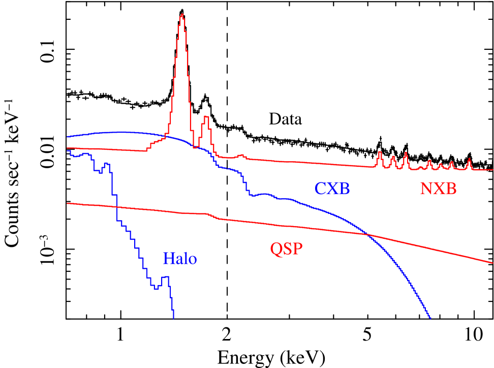
Figure 26: MOS1 spectrum from blank field observations in the 10^′-12^′ ring. Above 2 keV the spectrum is simpler.

Only the photon components (i.e. HALO and CXB) are multiplied by the effective area and absorbed by our Galaxy. The equivalent hydrogen column density along the line of sight, $N_{\mathrm{H}}$, is fixed to the 21 cm measurement (Dickey & Lockman 1990), averaged over all fields. We selected blank field observations pointed at high galactic latitude, therefore $N_{\mathrm{H}}$ is $<10^{21}$ cm^-2 and the absorption effect is negligible above 1 keV.

In the 0.7-10.0 keV band, the total model is composed of a thermal component (HALO), a power law (CXB), two broken power laws (QSP and NXB), and several Gaussians (fluorescence emission lines). The thermal model (APEC in XSPEC) parameters are: $\mathrm{k}T=0.197$ keV, $Z=1.0\;Z_{\odot}$, and $z=0.0$ (Kuntz & Snowden 2000). The slope of the CXB power law is fixed to 1.4 (De Luca & Molendi 2004) and the normalization is calculated at 3 keV to minimize the correlation with the slope. The QSP broken power law has a break energy at 5.0 keV; the slopes are fixed to 0.4 (below 5 keV) and 0.8 (above 5 keV). The model parameters for the internal background are the same as reported in Appendix A. In the 2.0-10.0 keV band the model is simpler, namely three power laws and several Gaussians, and more stable. The HALO component is negligible above 2 keV, the CXB model is the same as in the 0.7-10.0 keV band, the slope of the QSP power law is fixed to 1.0, and the model parameters for the internal background are those reported in Appendix A.

Most components have rather similar spectral shapes (see Fig. 26), therefore a high degree of parameter degeneracy is present. In such cases, it is useful to constrain as many parameters as possible. Events outside the field of view are exclusively due to the internal background, therefore the spectrum accumulated in this region provides a good estimate of the NXB normalization, $N_{\mathrm{NXB}}$. By analyzing closed (CL) observations we found that the ratio between $N_{\mathrm{NXB}}$ calculated in any two detector regions is independent of the particular observation:

$$\frac{N_{\mathrm{NXB}}(R_{1};O_{1})}{N_{\mathrm{NXB}}(R_{2};O_{1})}=\frac{N_{\mathrm{NXB}}(R_{1};O_{2})}{N_{\mathrm{NXB}}(R_{2};O_{2})}\,,$$ (7)

where $R_{1,2}$ are two detector regions and $O_{1,2}$ are two observations. By using the region outside the field of view (OUT), from Eq. 7 we estimate and fix $N_{\mathrm{NXB}}$ for each ring (R) of blank field (BF) observations:

$$N_{\mathrm{NXB}}(R;BF)=N_{\mathrm{NXB}}(R;CL)\times\frac{N_{\mathrm{NXB}}(OUT;BF)}{N_{\mathrm{NXB}}(OUT;CL)}\,.$$ (8)

Table 7: Best fit results for the analysis of blank field observations in the 10^′-12^′ ring.

Instr.	Filter	$N_{\mathrm{HALO}}$	$N_{\mathrm{QSP}}$	$N_{\mathrm{CXB}}^{\mathrm{a}}$
		[$10^{-4}$]	[$10^{-3}$]	[$10^{-2}$]
MOS1	THIN1	1.7$\pm$0.1	2.4$\pm$0.1	5.1$\pm$0.1
MOS2	THIN1	1.6$\pm$0.1	2.5$\pm$0.1	5.0$\pm$0.1
MOS1	MEDIUM	1.4$\pm$0.1	2.6$\pm$0.1	6.0$\pm$0.1
MOS2	MEDIUM	1.6$\pm$0.1	2.4$\pm$0.1	5.8$\pm$0.1

• ^a calculated at 3 keV.

In Table 7 we report the best fit values for the normalization of the HALO, $N_{\mathrm{HALO}}$, of the QSP, $N_{\mathrm{QSP}}$, and of the CXB, $N_{\mathrm{CXB}}$, in the 10^′-12^′ ring, for MOS1 and MOS2 instruments and for THIN1 and MEDIUM filters. Spectra are fitted in the 0.7-10.0 keV energy band. We stress the remarkably good agreement between MOS1 and MOS2, for all parameters. Moreover, we point out that, when comparing observations with different filters, values for $N_{\mathrm{HALO}}$ and $N_{\mathrm{QSP}}$ also agree, while values for $N_{\mathrm{CXB}}$ are significantly different ($\approx$ 20%) because of the cosmic variance ($\approx$ 15% expected for the considered solid angles).

By construction (see Eq. 1) $R_{\mathrm{SB}}$ is related to $N_{\mathrm{QSP}}$ so that the higher $R_{\mathrm{SB}}$, the higher $N_{\mathrm{QSP}}$. For observations that are not contaminated by QSP, we will measure $R_{\mathrm{SB}}\approx 1.0$ and $N_{\mathrm{QSP}}\approx 0.0$. Since $R_{\mathrm{SB}}$ values span a relatively small range (roughly between 1.0 and 1.5) we approximate the relation between $R_{\mathrm{SB}}$ and $N_{\mathrm{QSP}}$ with a linear function: $N_{\mathrm{QSP}}=A\times(R_{\mathrm{SB}}-1)$. The scaling factor, $A\approx 0.03$, is determined from the analysis of blank fields observations, for which we have measured $R_{\mathrm{SB}}=1.09\pm 0.01$ and $N_{\mathrm{QSP}}=(2.5\pm 0.1)\times 10^{-3}$. Thus, for each observation we model the bulk of the QSP component by deriving $N_{\mathrm{QSP}}$ from $R_{\mathrm{SB}}$ (see Sects. 3.2.1 and 3.2.2). In Sects. 5.1.3 and 5.2.3 we discuss possible systematics related to QSP and show that the linear approximation used above is satisfactory.

As mentioned in Sect. 3.2.1, we estimate the normalizations of the background components in the 10^′-12^′ ring and rescale them in the inner rings; when considering the 0.7-10.0 keV energy band, a simple rescaling by the area ratio is too rough and causes systematic errors, especially in the outer regions where cluster emission and background fluctuations become comparable. To overcome this problem, we proceed in the following manner: we fit blank field spectra, by fixing $N_{\mathrm{NXB}}$ and $N_{\mathrm{QSP}}$, and determine $N_{\mathrm{CXB}}$ and $N_{\mathrm{HALO}}$ best fit values. For each ring and instrument, we define a correction factor, $K(r)$:

$$K(r)=\frac{N_{\mathrm{obs}}}{N_{\mathrm{exp}}},$$ (9)

where $N_{\mathrm{obs}}$ is the best fit value that we have just obtained and $N_{\mathrm{exp}}$ is derived by rescaling the value measured in the 10^′-12^′ ring by the area ratio. In Table 8 we report the values for $K(r)$ for all cases.

Table 8: Correction factors.

Ring	HALO		CXB
	MOS1	MOS2	MOS1	MOS2
0′-2.75′	0.62	0.68	0.80	0.91
2.75′-4.5′	0.74	0.70	0.70	0.78
4.5′-6′	0.63	0.65	0.89	0.95
6′-8′	0.74	0.71	0.89	0.92

$K(r)$ is a second order correction, because the contribution of CXB and HALO components to the total flux is relatively small: when considering only the 0.7-2.0 keV band (i.e. the energy range in which these components are more intense), the HALO-to-total and the CXB-to-total flux ratios are $\approx$ 5% and $\approx$ 20% respectively. Thus, the effective correction is only of a few percent for both cases. Different observations have different centers in detector coordinates and the intensity of the various components depends on the particular observation; these facts could cause some discrepancies, however since we have analyzed a large number of blank and cluster fields, we expect only a few percent systematic effect on the mean profile. When considering the band above 2 keV, the statistical quality of the data is poorer, therefore the rescaling by the area ratio (i.e. no correction factor) can be considered a good approximation for both CXB and NXB. The QSP value is rescaled by the soft proton vignetting profile (Kuntz 2006) and does not require any correction factor.

Unfortunately, a precise characterization of the QSP component for EPIC-pn is not possible. Uncertainties on $N_{\mathrm{NXB}}$ are very large, because the region outside the EPIC-pn field of view is much smaller than the MOS one; the presence of a non negligible fraction of out-of-time events introduces a further complication. Moreover, the EPIC-pn background is much less stable than the EPIC-MOS one, especially below 2 keV. The EPIC-pn instrument has further drawbacks due to the electronic board near the detector: the NXB spatial distribution is not flat and the emission due to Ni-Cu-Zn lines (between $\approx$ 7.5 keV and $\approx$ 9.5 keV) is more intense in the outer rings. For these reasons, as mentioned in Sect. 3, we consider only EPIC-MOS data in our analysis.