The Binder Cumulant at the Kosterlitz-Thouless Transition

Martin Hasenbusch

Institut für Theoretische Physik, Universität Leipzig,

Postfach 100 920, D-04009 Leipzig, Germany

e-mail: Martin.Hasenbusch@itp.uni-leipzig.de

We study the behaviour of the Binder cumulant on finite square lattices at the Kosterlitz-Thouless phase transition. We determine the fixed point value of the Binder cumulant and the coefficient of the leading logarithmic correction. These calculations are supplemented with Monte Carlo simulations of the classical XY (plane rotator) model, the Villain model and the dual of the absolute value solid-on-solid model. Using the single cluster algorithm, we simulate lattices up to $L=4096$. For the lattice sizes reached, subleading corrections are needed to fit the data for the Binder cumulant. We demonstrate that the combined analysis of the Binder cumulant and the second moment correlation length over the lattice size allows for an accurate determination of the Kosterlitz-Thouless transition temperature on relatively small lattices. We test the new method at the example of the 2-component $\phi^{4}$ model on the lattice.

PACS numbers: 75.10.Hk, 05.10.Ln, 68.35.Rh

1 Introduction

Two dimensional systems with short range interactions and $O(2)$ symmetry undergo a Kosterlitz-Thouless (KT) phase transition [1]. This phase transition is of particular interest because of its peculiar nature and the large number of effectively two dimensional systems that are supposed to undergo such a transition.

Following the theorem of Mermin and Wagner [2] the magnetisation of two dimensional systems with short range interactions and a continuous symmetry vanishes at any finite temperature. Kosterlitz and Thouless [1] have argued that nevertheless two dimensional systems with $O(2)$ symmetry undergo a phase transition at a finite temperature. In the low temperature phase, the decay of the correlation function follows a power law. At a sufficiently high temperature, pairs of vortices unbind and disorder the system, resulting in a finite correlation length $\xi$; i.e. the correlation function decays exponentially. Starting from the seminal work of Kosterlitz and Thouless a rather solid theoretical understanding of the transition has been established. See e.g. refs. [3, 4]. Furthermore, there are exactly solved models [5, 6, 7, 8] that display the behaviour predicted by KT-theory.

This excellent theoretical understanding is contrasted by the fact that Monte Carlo studies of the KT-transition are notoriously difficult. These difficulties are related with logarithmic corrections that are present in the neighbourhood of the transition.

In Monte Carlo studies of critical phenomena, renormalization group invariant quantities, which are also called phenomenological couplings, are very useful tools. In finite size scaling (FSS), they allow to locate the transition point, to determine the nature of the transition and, in the case of a second order transition, to determine the critical exponent $\nu$ of the correlation length. The prototype of such a quantity is the so called Binder cumulant

$$U=\frac{\langle(\vec{m}^{2})^{2}\rangle}{\langle\vec{m}^{2}\rangle^{2}}\;\;,$$ (1)

where $\vec{m}$ is the magnetisation of the system . While the Binder cumulant is a standard tool in the study of second order transitions, only a few authors have advocated its use in the case of a KT-transition [9, 10]. This is due to the fact that little is known about the behaviour of the Binder cumulant in the neighbourhood of the KT-transition. The main purpose of the present paper is to fill this gap.

The outline of the paper is the following: First we define the models and the observables that we study. Next we summarize the results from KT-theory which are relevant to our problem. Then we derive the fixed point value of the Binder cumulant and the coefficient of the leading logarithmic correction. We discuss our Monte Carlo simulations of the XY model, the Villain model and the dual of the absolute value solid-on-solid (ASOS) model at the KT-transition. The Monte Carlo results for the Binder cumulant, the second moment correlation length and the helicity modulus are confronted with the theoretical predictions. Based on this discussion, we propose to determine the transition temperature of a model which is supposed to undergo a KT-transition by simultaneously matching the values of the second moment correlation length and the Binder cumulant with those obtained for the three models studied in this paper. This method is tested at the example of the two-component $\phi^{4}$ model on the square lattice. Finally we give our conclusions.

2 The models

We study the XY model on the square lattice and two generalizations of it: The Villain model and the dual of the absolute value solid-on-solid model. This allows us to check the universality of the behaviour of the Binder cumulant and other phenomenological couplings. The Boltzmann factor of these models can be written as a product of weights for pairs of nearest neighbour sites on the lattice. In all three cases we have

$$B(\{\vec{s}_{x}\})=\prod_{x,\mu}w(\theta_{x,\mu})\;\;,$$ (2)

where $\theta_{x,\mu}$ is the angle between nearest neighbour spins $\vec{s}_{x}$ and $\vec{s}_{x+\hat{\mu}}$. The spin $\vec{s}_{x}$ is a unit vector with two real components, $x=(x_{1},x_{2})$ labels the sites on the square lattice, where $x_{1}\in\{1,2,...,L_{1}\}$ and $x_{2}\in\{1,2,...,L_{2}\}$ , $\mu$ gives the direction on the lattice and $\hat{\mu}$ is a unit-vector in the $\mu$-direction. We consider periodic boundary conditions in both directions. The weight function is periodic: $w(\theta)=w(\theta+2n\pi)$ for any integer $n$. The partition function is given by the integral

$$Z=\int\prod_{x}[\mbox{d}s_{x}^{(1)}\mbox{d}s_{x}^{(2)}\delta(\vec{s}_{x}^{\;2}-1)]\;B(\{\vec{s}_{x}\})\;\;.$$ (3)

Note that two dimensional XY-models on square lattices with Boltzmann factors given by eq. (2) can be exactly mapped onto so called solid-on-solid (SOS) models. For a detailed discussion see ref. [11]. The variables $h_{x}$ of an SOS model are integers living on the sites $x$ of a square lattice. The Boltzmann factor of these models can be written as a product over nearest neighbour pairs

$$\tilde{B}(\{\vec{h}_{x}\})=\prod_{x,\mu}\tilde{w}(|h_{x}-h_{x+\hat{\mu}}|)\;\;,$$ (4)

The relation between the weight function of an SOS model and its dual XY model is given by

$$w(\theta)=\sum_{n=-\infty}^{\infty}\tilde{w}(n)\cos(n\theta)$$ (5)

and

$$\tilde{w}(n)=\frac{1}{2\pi}\int_{-\pi}^{\pi}\mbox{d}\theta\;w(\theta)\cos(n\theta)\;.$$ (6)

The weight of the standard XY model (or plane rotator model) is given by

$$w_{XY}(\theta_{x,\mu})=\exp(\beta\cos(\theta_{x,\mu}))=\exp(\beta\;\vec{s}\cdot\vec{s}_{x+\hat{\mu}})\;,$$ (7)

where $\beta$ is the inverse temperature. In the case of the other two models it is simpler to give the weights for the SOS representation. The Villain model is dual to the discrete Gaussian solid-on-solid (DGSOS) model. Its weight is given by

$$\tilde{w}_{DGSOS}(n)=\exp(-\tilde{\beta}n^{2})\;.$$ (8)

It follows

$$w_{Villain}(\theta)=\sum_{n=-\infty}^{\infty}\exp(-\tilde{\beta}n^{2}+in\theta)=c\sum_{m=-\infty}^{\infty}\exp\left(-\frac{\beta}{2}(\theta-2\pi m)^{2}\right)\;\;,$$ (9)

where $\beta=1/(2\tilde{\beta})$ and $c=\sqrt{2\pi\beta}$. For a proof of this equation see e.g. appendix A.1 of ref. [12].

The weight of the absolute value solid-on-solid (ASOS) model is given by

$$\tilde{w}_{ASOS}(n)=\exp(-\tilde{\beta}|n|)\;\;.$$ (10)

The KT-temperatures of these models have been accurately determined [13, 14] by an RG mapping of these models with the exactly solved body centred cubic solid-on-solid (BCSOS) model [5, 6, 7, 8]:

$$\beta_{KT}^{XY} = 1.1199(1)\;\;\;\;\;\;\;\;\;\;\;\;\;b_{m}^{XY}=0.93(1)\;,$$

$$\beta_{KT}^{Villain} = 0.75154(23)\;\;\;\;\;\;b_{m}^{Villain}=0.32(1)\;,$$

$$\tilde{\beta}_{KT}^{ASOS} = 0.80608(2)\;\;\;\;\;\;\;\;\;b_{m}^{ASOS}=2.78(3)\;.$$ (11)

In addition to the (inverse) temperature of the KT-transition we give the scale factor $b_{m}$ that is needed to match the given model with the BCSOS model. E.g. results for the ASOS model at the KT-transition obtained at the lattice size $L_{ASOS}$ match with the BCSOS model at the transition at the lattice size $L_{BCSOS}=L_{ASOS}/b_{m}^{ASOS}$.

3 The observables

In this section we shall summarize the definitions of the observables that we have measured in our simulations. The total magnetisation is defined by

$$\vec{m}=\sum_{x}\vec{s}_{x}\;\;.$$ (12)

The magnetic susceptibility is then given by

$$\chi=\frac{1}{L^{2}}\langle\vec{m}^{2}\rangle\;\;,$$ (13)

where $\langle\ldots\rangle$ denotes the expectation value with respect to the Boltzmann factors defined in the previous section. For completeness we repeat the definition of the Binder cumulant

$$U=\frac{\langle(\vec{m}^{2})^{2}\rangle}{\langle\vec{m}^{2}\rangle^{2}}\;.$$ (14)

The second moment correlation length on a lattice of the size $L^{2}$ is defined by

$$\xi_{2nd}=\frac{1}{2\sin(\pi/L)}\left(\frac{\chi}{F}-1\right)^{1/2}\;,$$ (15)

where $\chi$ is the magnetic susceptibility as defined above and

$$F=\frac{1}{L^{2}}\sum_{x,y}\langle\vec{s}_{x}\vec{s}_{y}\rangle\cos(2\pi(y_{1}-x_{1})/L)$$ (16)

is the Fourier transform of the correlation function at the smallest non-vanishing momentum. In our simulations we have measured $F$ for both directions of the lattice to reduce the statistical error.

The helicity modulus $\Upsilon$ gives the reaction of the system under a torsion [15]. To define the helicity modulus we consider a system, where rotated boundary conditions in one direction are introduced: For pairs $x,x+\hat{\mu}$ of nearest neighbour sites on the lattice with $x_{1}=L_{1}$ and $\mu=1$ the weight $w(\theta_{x,\mu})$ is replaced by $w(\theta_{x,\mu}+\alpha)$. The helicity modulus is then defined by the second derivative of the free energy with respect to $\alpha$ at $\alpha=0$

$$\Upsilon=-\frac{L_{1}}{L_{2}}\left.\frac{\partial^{2}\ln Z(\alpha)}{\partial\alpha^{2}}\right|_{\alpha=0}\;\;.$$ (17)

Note that we have skipped a factor one over temperature in our definition of the helicity modulus to obtain a dimensionless quantity. In the case of the standard XY model it is easy to write the helicity modulus as an observable of the system at $\alpha=0$ [16]. For $L_{1}=L_{2}=L$ we get

$$\Upsilon=\frac{\beta}{L^{2}}\left\langle\vec{s}_{x\phantom{\hat{1}}}\vec{s}_{x+\hat{1}}\right\rangle-\frac{\beta^{2}}{L^{2}}\left\langle\left(s_{x\phantom{\hat{1}}}^{(1)}s_{x+\hat{1}}^{(2)}-s_{x\phantom{\hat{1}}}^{(2)}s_{x+\hat{1}}^{(1)}\right)^{2}\right\rangle\;\;.$$ (18)

Note that this equation is not valid for the other two models that we have studied.

4 KT-theory

At low temperatures, fluctuations are suppressed and we might expand the weight as

$$-\ln(w(\theta))=const-\frac{\beta_{SW}}{2}\theta^{2}+\ldots$$ (19)

Note that for the models discussed above, $w(\theta)$ is an even function that assumes its maximum at $\theta=0$. Using this approximation we arrive at the exactly solvable Gaussian model (or free field theory in the language of high energy physics):

$$Z_{SW}=\int\prod_{x}[\mbox{d}\theta_{x}]\delta\left(\sum_{x}\theta_{x}\right)\exp(-H_{SW})$$ (20)

with

$$H_{SW}=\frac{\beta_{SW}}{2}\sum_{x,\mu}(\theta_{x}-\theta_{x+\hat{\mu}})^{2}\;\;.$$ (21)

Note that the $\delta$-function in eq. (20) is needed to render the integral finite. For the solution of this model see e.g. Appendix A of ref. [3] or textbooks; e.g. ref. [17].

In the spin-wave approximation, vortices that drive the KT phase transition are absent. A careful analysis shows that they are, in an RG-sense, irrelevant for $\beta_{SW}\geq\frac{2}{\pi}$ [3, 4]. I.e. the large distance behaviour of systems at the KT-transition is given by the spin-wave model at $\beta_{SW}=\frac{2}{\pi}$.

For the discussion of the RG-flow in the neighbourhood of the KT-transition it is convenient to define $x=\pi\beta_{SW}-2$. At the KT-transition, $x$ behaves as [3, 4]

$$x(l)=\frac{1}{\ln l+C}+\ldots\;,$$ (22)

where $C$ is an integration constant and $l$ is a length scale. In the case of finite size scaling, we identify the lattice size $L$ with this scale.

Leading corrections to the asymptotic behaviour of correlation functions at the KT-transition can be obtained by computing the correlation function in the spin-wave approximation for $\beta_{SW}$ given by eq. (22).

Along these lines we obtained [18]

$$\Upsilon_{L^{2},transition}=0.63650817819...+\frac{0.318899454...}{\ln L+C}+\;...$$ (23)

for the helicity modulus. Note that in the literature (see e.g. eq. (4) of ref. [19]) often $\Upsilon=\frac{2}{\pi}+\frac{1}{\pi}\frac{1}{(\ln L+C)}\ldots$ is given. The small difference is due to the fact that in ref. [18] contributions from configurations with non-zero winding number are taken into account. For the second moment correlation length over the lattice size we obtained [18]

$$\left.\frac{\xi_{2nd}}{L}\right|_{L^{2},transition}=0.7506912...+\frac{0.212430...}{\ln L+C}+\;...\;\;.$$ (24)

The subscript refers to the fact that the result holds for a lattice of the size $L_{1}=L_{2}=L$ with periodic boundary conditions at the KT-transition. Furthermore the couplings between the spins have to be the same in both directions as it is the case here.

Computing four-point functions $\langle(\vec{s}_{x}\cdot\vec{s}_{y})(\vec{s}_{u}\cdot\vec{s}_{v})\rangle$ for all $y-x$, $u-x$ and $v-x$ from the propagator of the Gaussian model requires a triple sum over all points of the lattice. Therefore we could not reach sufficiently large lattice sizes this way. To avoid this problem, we performed Monte Carlo simulations of the Gaussian model instead.

4.1 Monte Carlo Simulation of the Gaussian Model

First note that $\beta_{SW}$ in eq. (21) can be absorbed into the field variable by $\phi_{x}=\beta_{SW}^{1/2}\theta_{x}$. In terms of the new field variable the Hamiltonian becomes

$$H_{SW}=\frac{1}{2}\sum_{x,\mu}(\phi_{x}-\phi_{x+\hat{\mu}})^{2}\;\;.$$ (25)

The spin configurations are given by

$$\vec{s}_{x}(n_{1},n_{2})=\left(\cos(\beta_{SW}^{-1/2}\phi_{x}+\psi_{x}(n_{1},n_{2})),\sin(\beta_{SW}^{-1/2}\phi_{x}+\psi_{x}(n_{1},n_{2}))\right)\;,$$ (26)

where $\psi_{x}(n_{1},n_{2})=2\pi(n_{1}x_{1}+n_{2}x_{2})/L$ takes into account windings of the spin configuration, where $n_{1}$ and $n_{2}$ are integers. As discussed in section 3.2 of ref. [18], expectation values of an observable $A$ in the spin wave approximation on a lattice with periodic boundary conditions are given by

$$\langle A(\{\vec{s}\})\rangle_{SW}=\frac{\sum_{n_{1},n_{2}}W(n_{1},n_{2})\langle A(\{\vec{s}\}_{n_{1},n_{2}})\rangle}{\sum_{n_{1},n_{2}}W(n_{1},n_{2})}\;\;,$$ (27)

where

$$\langle A(\{\vec{s}\}_{n_{1},n_{2}})\rangle=\frac{\int\prod_{x}[\mbox{d}\phi_{x}]\delta(\sum_{x}\phi_{x})\exp(-H_{SW}(\{\phi\}))A(\{\vec{s}\}_{n_{1},n_{2}})}{\int\prod_{x}[\mbox{d}\phi_{x}]\delta(\sum_{x}\phi_{x})\exp(-H_{SW}(\{\phi\}))}\;\;.$$ (28)

The weights for the different winding numbers are given by

$$W(n_{1},n_{2})=\exp\left(-2\pi^{2}\beta_{SW}[n_{1}^{2}+n_{2}^{2}]\right)\;\;.$$ (29)

Note that these weights do not depend on $L$ and therefore also non-zero winding numbers contribute to the asymptotic behaviour. In our simulations we have only taken into account the winding numbers $(n_{1},n_{2})=$ $(-1,0),(1,0),(0,-1)$ and $(0,1)$. The weight for these winding numbers is $0.000003487\ldots$ at $\beta_{SW}=2/\pi$. This weight is rather small. However it turns out that at the level of accuracy that we have reached these windings have to be taken into account. Higher winding numbers can be safely ignored.

In momentum space, the degrees of freedom of the Gaussian model decouple. Therefore one can directly generate a field configuration, using e.g. the Box-Muller algorithm, in momentum space with the correct probability density. Then one can perform a Fourier transformation to obtain the configuration in real space.

Since we had the program code available, we used a different approach: We generated the configurations directly in real space, using a mixture of the local Metropolis, the overrelaxation and a single cluster version [20] of the valley to mountain reflection (VMR) algorithm [21]. Due to the use of the cluster algorithm, there should be no slowing down and therefore our choice should have a similar performance as the one sketched above.

In an elementary step of the Metropolis algorithm we propose to change the field at the site $x$ as

$$\phi_{x}^{\prime}=\phi_{x}+2(r-1/2)\;,$$ (30)

were $r$ is a random number that is uniformly distributed in $[0,1]$. The proposal is accepted with the probability $A=\mbox{min}[1,\exp(-\Delta H)]$. An elementary step of the overrelaxation algorithm is given by

$$\phi_{x}^{\prime}=2\frac{\sum_{y.nn.x}\phi_{y}}{4}-\phi_{x}\;,$$ (31)

where $y.nn.x$ indicates that $y$ is a nearest neighbour of $x$. Note that this update does not change the value of the Hamiltonian. In both cases, the Metropolis update and the overrelaxation update, we go through the lattice in lexicographic order. Going through the lattice once with the local update is called sweep.

The variant of the VMR algorithm that we have used here is given by the following steps:

• Chose randomly a site $x$ of the lattice. The reference hight for the update is then given by $h_{0}=\phi_{x}$. All fields $\phi_{z}$ that reside on sites $z$ that belong to the cluster are updated as

  $$\phi_{z}^{\prime}=2h_{0}-\phi_{z}\;.$$ (32)

  I.e. the field is reflected at $h_{0}$.

• Chose randomly a site $y$ of the lattice as the starting point of the single cluster. The cluster consists of all sites $z$ that are connected with $y$ by a chain of frozen links. The links that are not frozen are called deleted. The probability to delete a link $v,\mu$ is given by

  $$p_{d}(v,\mu)=\mbox{min}[1,\exp(-2(\phi_{v}-h_{0})(\phi_{v+\hat{\mu}}-h_{0}))]\;\;.$$ (33)

  Note that in this equation both $\phi_{v}$ and $\phi_{v+\hat{\mu}}$ are taken before the update.

We performed the updates in the following sequence: One Metropolis sweep, one overrelaxation sweep and finally a VMR single cluster update. The average size of the single cluster is about 1/3 of the lattice, independent of the lattice size. Integrated autocorrelation times of the magnetic susceptibility (13,27) at $\beta_{SW}=2/\pi$ are about 2.8 for $L=32$ and increase to about 5 for $L=512$, where the time unit is one update sequence as specified above.

In our production runs, the measurements are separated by 5 such sequences. We performed $20$, $20$, $12$, $5$ and $2.2$ $\times 10^{7}$ measurements for $L=32$, $64$, $128$, $256$ and $512$, respectively. In total, these simulations took about 10 month of CPU time on a 3 GHz Pentium 4 CPU.

In order to compute $\lim_{L\rightarrow\infty}U_{4}$ at the KT-transition, we have set $\beta_{SW}=\frac{2}{\pi}$ in eq. (26). In addition we have used $\beta_{SW}=\left(\sqrt{\frac{2}{\pi}}+0.0001\right)^{2}$ and $\beta_{SW}=\left(\sqrt{\frac{2}{\pi}}-0.0001\right)^{2}$ to compute the derivative of $\lim_{L\rightarrow\infty}U_{4}$ with respect to $\beta_{SW}$ at $\beta_{SW}=\frac{2}{\pi}$. Note that we have used the same set of $\phi$ configurations for the three values of $\beta_{SW}$. Our results are summarized in table 1.

A brief remark on non-zero winding numbers: Taking only zero winding configurations, $U_{4}$ is about $0.000013$ smaller than with the non-zero winding numbers taken into account. I.e. the contribution of non-zero winding numbers is a little larger than our statistical error.

Table 1: Results for the Binder cumulant $U_{4}$ in the spin wave approximation at $\beta_{SW}=2/\pi$ and its derivative with respect to $\beta_{SW}$. In the last row we give the result for the limit $L\rightarrow\infty$.

$L$	$U_{4}$ xxx	$\mbox{d}U_{4}/\mbox{d}{\beta_{SW}}$
32	1.018554(2)	–0.057529(7)
64	1.018298(2)	–0.056679(7)
128	1.018217(3)	–0.056394(9)
256	1.018200(5)	–0.056332(15)
512	1.018199(8)	–0.056297(25)
$\infty$	1.018192(6)	–0.056303(16)

In order to obtain a result for the limit $L\rightarrow\infty$ we have fitted the results to the ansatz $X(L)=X(\infty)+cL^{-2}$, where $X$ is either the Binder cumulant or its derivative. Our final results are taken from the fit that includes the lattice sizes $L=128$, $256$ and $512$. These results are consistent within error bars with those obtained from $L=64$ and $128$. Hence the systematic error due to higher order corrections should be quite small.

Plugging the result for the derivative of $U_{4}$ into eq. (22) we arrive at

$$U_{4,L^{2},transition}=1.018192(6)-\frac{0.017922(5)}{\ln L+C}+...\;,$$ (34)

where we should note again that the result only holds for a lattice with $L_{1}=L_{2}=L$ with periodic boundary conditions at the KT-transition. Furthermore the couplings between the spins have to be the same in both directions as it is the case here.

5 Monte Carlo Simulations

In this section we discuss the details of our Monte Carlo simulations of the XY, the Villain and the dual of the ASOS model.

5.1 Details of the Simulations

We have simulated the XY model, the Villain and the dual of the ASOS model at the best estimates of the KT-temperature given in eq. (11). In our simulations we have used the single cluster algorithm [20]. Let us briefly summarize the steps of the cluster update:

• Chose a direction:

  $$\vec{d}=(\cos(2\pi r),\sin(2\pi r))\;,$$ (35)

  where $r$ is a random number which is uniformly distributed in $[0,1]$ . All spins $\vec{s}_{x}$ that reside on sites $x$ that belong to the cluster will be updated as

  $$\vec{s}_{x}^{\;\;{}^{\prime}}=\vec{s}_{x}-2(\vec{d}\cdot\vec{s}_{x})\vec{d}\;\;,$$ (36)

• Chose randomly a site $y$ as starting point of the single cluster. All sites $x$ belong to the cluster that are connected by a frozen chain of links with the site $y$. A link that is not frozen is called deleted. The probability to delete a link $x,\mu$ is given by

  $$p_{d}(x,\mu)=\mbox{min}\left[1,\frac{w\left(\vec{s}_{x}\cdot\vec{s}_{x+\mu}-2(\vec{d}\cdot\vec{s}_{x})(\vec{d}\cdot\vec{s}_{x+\mu})\right)}{w(\vec{s}_{x}\cdot\vec{s}_{x+\mu})}\right]\;\;.$$ (37)

  Note that in this equation both $\vec{s}_{x}$ and $\vec{s}_{x+\mu}$ are taken before the update.

Our first set of simulations of the XY-model was performed with the single cluster algorithm alone. In these simulations we have used the G05CAF random number generator of the NAG-library. We simulated the lattice sizes $L=$ $16$, $32$, $64$, $128$, $256$, $512$, $1024$, $2048$ and $4096$. For $L\leq 1024$ we performed $5\times 10^{6}$ measurements. For $L=2048$ and $L=4096$ we performed $2.5\times 10^{6}$ and $1\times 10^{6}$ measurements, respectively. In all these cases, we performed 10 single cluster updates for one measurement. In total, these simulations took a bit more than 7 month of CPU time on a 3 GHz Pentium 4 CPU.

Later we added simulations for $L=12$, $24$, $48$, $96$, $192$, $384$ and $768$. As random number generator we have used here the SIMD-oriented Fast Mersenne Twister (SFMT) [22] generator. In particular we use the function genrand$\_$res53() that produces double precision output.

In these simulations we performed overrelaxation updates in addition to the cluster updates. An overrelaxation update of the spin at the site $x$ is given by

$$\vec{s}_{x}^{\;\;{}^{\prime}}=\vec{s}_{x}-2\frac{\vec{S}_{x}\cdot\vec{s}_{x}}{\vec{S}_{x}^{2}}\vec{S}_{x}\;\;,$$ (38)

where

$$\vec{S}_{x}=\sum_{y.nn.x}\vec{s}_{y}\;\;,$$ (39)

where $y.nn.x$ means that $y$ is a nearest neighbour of $x$. It is easy to check that this update keeps the value of the Hamiltonian constant.

For $L\leq 192$ we performed $10^{7}$ measurements. For each measurement we performed 10 single cluster updates and 10 overrelaxation sweeps. For $L=384$ and $768$ we performed $9\times 10^{6}$ measurements. In these two cases we performed 10 single cluster updates and 5 overrelaxation sweeps for each measurement. In total, these simulations took a bit more than 4 month of CPU time on a 3 GHz Pentium 4 CPU.

In the case of the Villain model and the dual of the ASOS model, we have implemented the weight function $w(\vec{s}_{x}\cdot\vec{s}_{x+\hat{\mu}})$ for the links as a table with 100001 entries for the arguments $-1,-0.99998,-0.99996,...,1$. Then, for a given value of the argument, we linearly interpolate between the two closest values contained in the table. This way, the maximal error in ratios of the weight for links is about $10^{-9}$ and $1.4\times 10^{-9}$ for the Villain model and the dual of the ASOS model, respectively. For all simulations of the Villain model and the dual of the ASOS model we have used the SFMT random number generator.

The Villain model was simulated on lattices of the size $L=16$,$32$,$64$,$128$, $256$,$512$,$1024$ and $2048$. For $L\leq 128$ we performed $10^{7}$ measurement for each lattice size. The statistics for the larger lattice sizes is about $8.2\times 10^{6}$, $5.1\times 10^{6}$, $3.1\times 10^{6}$ and $1.4\times 10^{6}$ measurements for $L=256$, $512$, $1024$ and $2048$, respectively. In all cases, we performed 10 single cluster updates per measurement. In total, the simulations of the Villain model took about 3 month of CPU time on a 3 GHz Pentium 4 CPU.

In the case of the dual of the ASOS model we have simulated lattices of the size $L=$ 16,24,32,48,64,96,128,192,256,384,512,768 and 1024. Also here we performed 10 single cluster updates per measurement. The number of measurements was $2\times 10^{7}$ for all lattice sizes up to $L=512$. We performed $1.27\times 10^{7}$ and $1.1\times 10^{7}$ measurements for $L=768$ and $L=1024$, respectively. In total, the simulations of the dual of the ASOS model took a little less than 10 month of CPU time on a 3 GHz Pentium 4 CPU.

For all cases, the integrated autocorrelation times for e.g. the magnetic susceptibility are close to one in units of measurements. We have discarded at least the first 1000 measurements for equilibration. Given the small autocorrelation times this is by far sufficient.

5.2 Analysis of the Data

First we have analysed the data for the helicity modulus of the XY model. We compared these data with the behaviour given by eq. (23). To this end, we have approximated the helicity modulus in the neighbourhood of the simulation point by the Taylor expansion around the simulation point to linear order. I.e. we have used the ansatz

$$\Upsilon(1.1199)+\left.\frac{\mbox{d}\Upsilon}{\mbox{d}\beta}\right|_{\beta=1.1199}\Delta\beta=0.63650817819+\frac{0.318899454}{\ln L+C}$$ (40)

with the two parameters $\Delta\beta$ and $C$ to fit our data for the helicity modulus. The results of these fits are summarized in table 2. In these fits we have used all data starting from some minimal lattice size $L_{min}$ up to the maximal size available. In order to get a $\chi^{2}/$d.o.f. close to one, $L_{min}=384$ is needed. The result for $\Delta\beta$ is decreasing with increasing $L_{min}$. Starting from $L_{min}=384$, the result for $\Delta\beta$ is consistent within error-bars with $\Delta\beta=0$; i.e. our previous estimate for $\beta_{KT}$. Since corrections to the ansatz (40) are expected to decay slowly with increasing lattice size, it is difficult to give a reliable estimate of systematic errors. Therefore we abstain from giving a final estimate for $\beta_{KT}$ obtained from these fits.

Table 2: Fits of the helicity modulus $\Upsilon$ for the XY model with the ansatz (40). $L_{min}$ is the minimal lattice size that is included in the fit. $C$ and $\Delta\beta$ are the parameters of the fit. For a discussion see the text.

$L_{min}$	xx $C$	$\Delta\beta$	$\chi^{2}/$d.o.f.
96	1.001(6)	0.00049(2)	9.83
128	1.044(10)	0.00038(3)	6.22
192	1.067(11)	0.00033(3)	4.51
256	1.124(19)	0.00021(4)	2.53
384	1.167(24)	0.00013(5)	0.56
512	1.170(37)	0.00013(7)	0.74
784	1.191(51)	0.00009(9)	0.93

Next we have studied the second moment correlation length $\xi/L$ of the XY-model using the ansatz

$$\frac{\xi(1.1199)}{L}+\frac{1}{L}\left.\frac{\mbox{d}\xi}{\mbox{d}\beta}\right|_{\beta=1.1199}\Delta\beta=0.7506912+\frac{0.212430}{\ln L+C}\;.$$ (41)

Our results are summarized in table 3. In contrast to the helicity modulus, the $\chi^{2}$/d.o.f. is rather small already for $L_{min}=32$. Also the dependence of the result for $\Delta\beta$ on $L_{min}$ is much smaller than for the helicity modulus. Hence the amplitude of corrections to the ansatz should be much smaller than for the helicity modulus. On the other hand, for a given $L_{min}$ the statistical error of $\Delta\beta$ obtained from $\xi/L$ is about three times larger than that from $\Upsilon$.

Since $\Delta\beta$ as a function of $L_{min}$ behaves quite differently for $\xi/L$ and $\Upsilon$ we might take the difference as an estimate of the error due to the higher order contributions missing in the ansätze (40,41). Starting from $L_{min}=384$ the result for $\Delta\beta$ from helicity modulus is consistent within statistical errors with that obtained from $\xi/L$ for $L_{min}\geq 32$. Hence the systematic error should not be larger than the statistical error for these $L_{min}$. Therefore we quote $\beta_{KT}=1.1200(1)$ as final result for the inverse of the KT-transition temperature of the XY model from the combined analysis of $\Upsilon$ and $\xi/L$.

Table 3: Fits of the correlation length over the lattice size $\xi/L$ for the XY model using the ansatz (41). $L_{min}$ is the minimal lattice size that is included in the fit. $C$ and $\Delta\beta$ are the parameters of the fit. For a discussion see the text.

$L_{min}$	$C$	$\Delta\beta$	$\chi^{2}/$d.o.f.
32	1.63(2)	0.00007(5)	1.61
48	1.64(2)	0.00005(6)	1.71
64	1.64(3)	0.00004(7)	1.89
96	1.62(3)	0.00009(7)	1.82
128	1.64(4)	0.00005(9)	2.02
192	1.60(5)	0.00012(10)	1.94

Next we have fitted $\xi/L$ for the dual of the ASOS model with the analogue of the ansatz (41); I.e. $1.1199$ is replaced by $0.80608$ as argument of $\xi$ and its derivative. The results are summarized in table 4. The $\chi^{2}/$d.o.f. becomes smaller than one starting from $L_{min}=48$. Also starting from $L_{min}=48$, the result for $\Delta\beta$ depends very little on $L_{min}$. These fits suggest the new estimate $\tilde{\beta}_{KT}=0.80605(2)$. This result is consistent with that of ref.[14].

Table 4: Analogue of table 3 for the ASOS model.

$L_{min}$	$C$	$\Delta\beta$	$\chi^{2}/$d.o.f.
32	0.493(6)	–0.000098(11)	10.50
48	0.545(8)	–0.000035(13)	00.59
64	0.548(11)	–0.000031(15)	00.64
96	0.548(16)	–0.000032(19)	00.75
128	0.543(20)	–0.000036(22)	00.88

Finally we have fitted the data for $\xi/L$ for the Villain model with the analogue of the ansatz (41). The results are summarized in table 5. We get $\chi^{2}/$d.o.f. close to one starting from $L_{min}=32$. These fits suggest as estimate for the inverse of the KT-transition temperature $\beta_{KT}=0.7517(2)$. Again this result is consistent with that of ref.[14].

Table 5: Analogue of table 3 for the Villain model.

$L_{min}$	$C$	$\Delta\beta$	$\chi^{2}/$d.o.f.
16	2.78(2)	–0.00009(8)	2.44
32	2.72(3)	0.00006(9)	1.30
64	2.69(5)	0.00014(12)	1.38
128	2.69(7)	0.00014(17)	1.85

Next let us discuss the results for the parameter $C$ in eq. (41). As our final results we take $C_{XY}=1.62(3)$ from the fit with $L_{min}=96$ for the XY model, $C_{Villain}=2.69(5)$ from $L_{min}=64$ for the Villain model and $C_{ASOS}=0.54(2)$ from $L_{min}=128$ for the dual of the ASOS model. The differences of these constants for different models should be given by the logarithm of ratios of the scale factors $b_{m}$ summarized in eq. (11). In particular we get $C_{Villain}-C_{ASOS}=2.15(5)$ to be compared with $\log(b_{m,ASOS}/b_{m,Villain})=2.16(3)$, $C_{Villain}-C_{XY}=1.07(6)$ to be compared with $\log(b_{m,XY}/b_{m,Villain})=1.07(3)$ and finally $C_{XY}-C_{ASOS}=1.08(4)$ to be compared with $\log(b_{m,ASOS}/b_{m,XY})=1.10(2)$. I.e. the results for $C$ are fully consistent with the relative scale factors $b_{m}$ obtained in ref.[14].

Next we discuss the behaviour of the Binder cumulant. In fig. 1 we have plotted the Binder cumulant at the old estimates of $\beta_{KT}$ summarized in eq. (11) as a function of $L_{XY}=L_{model}b_{m,model}/b_{m,XY}$. The data from the three different models fall nicely on top of each other, indicating a universal behaviour. From the leading behaviour, eq. (34), we would expect that the Binder cumulant is increasing with increasing lattice size $L$. However we observe quite the opposite. For all three models, it is decreasing and apparently reaches a stable value $\approx 1.0170$ for large lattice sizes.

Within the KT-picture this might be explained by large $O(1/(\ln L)^{2})$ correction due to the effect of vortex pairs with a distance $\approx L/2$. Configurations with such a vortex pair have a much smaller magnetisation than those without. Therefore the appearance of such vortices enlarges the value of the Binder cumulant $U_{4}$. Since $\beta_{SW}$ is monotonically decreasing with increasing $L$, the effect seen in the Binder cumulant can only be explained by the effect of vortices.

Based on this observation, we have fitted the Binder cumulant at the estimate of $\beta_{KT}$ given in eq. (11) with the ansatz

$$U_{4}(L)=1.018192-\frac{0.017922}{\ln L+C}+\frac{c_{2}}{(\ln L+C)^{2}}\;\;,$$ (42)

where $C$ and $c_{2}$ are the free parameters of the fit. Results for these fits for the XY model, the Villain model and the dual of the ASOS model are given in tables 6, 7 and 8, respectively.

$\chi^{2}/$d.o.f. becomes smaller close to one for $L_{min}=96$, $32$ and $96$ for the XY model, the Villain model and the dual of the ASOS model, respectively. For these values of $L_{min}$, the results for $c_{2}$ of the XY model and the Villain model are fully consistent, supporting the universality of the value of this coefficient. The result for the dual of the ASOS model is slightly smaller than that for the other two models. This small difference might be caused by higher order corrections or might be due to the uncertainty in the estimate of $\beta_{KT}$. To check the latter, we have repeated the fits for the central estimate for $\beta_{KT}$ given in eq. (11) plus or minus the error-bar. Let us give only a few results with $\chi^{2}$/d.o.f. smaller than two: For the XY at $\beta=1.1200$ and $L_{min}=96$ we get $C=0.006(36)$ and $c_{2}=0.06764(31)$. For the Villain model at $\beta=0.75177$ and $L_{min}=32$ we get $C=1.040(35)$ and $c_{2}=0.06699(32)$. And finally, for the dual of the ASOS model at $\tilde{\beta}=0.80606$ and $L_{min}=96$ we get $C=-1.193(10)$ and $c_{2}=0.06730(17)$. I.e. the small difference in the values of $c_{2}$ observed above can indeed be explained by the uncertainty of the estimate of $\beta_{KT}$.

Finally let us compare the differences in $C$ for the three models with the results for $b_{m}$ given in eq. (11). Using the results obtained for $L_{min}=96$, $32$ and $96$ for the XY-model at $\beta=1.1199$, the Villain model at $\beta=0.75154$ and the dual of the ASOS model at $\tilde{\beta}=0.80608$, respectively, we get: $C_{Villain}-C_{ASOS}=2.33(4)$, $C_{XY}-C_{ASOS}=1.25(4)$ and $C_{Villain}-C_{XY}=1.08(5)$. The two differences that involve the dual of the ASOS model are by about $0.15$ too large compared with the result obtained from $b_{m}$. The difference $C_{Villain}-C_{XY}$ is fully consistent with that obtained from $b_{m}$. Taking the result for the XY-model at $\beta=1.1200$, the Villain model at $\beta=0.75177$ and the dual of the ASOS model at $\tilde{\beta}=0.80606$ instead, we get $C_{Villain}-C_{ASOS}=2.23(4)$, $C_{XY}-C_{ASOS}=1.20(4)$ and $C_{Villain}-C_{XY}=1.03(5)$. I.e. the deviation from the expected result is much reduced.

Table 6: Fits of the Binder cumulant of the XY model at $\beta=1.1199$ with the ansatz (42).

$L_{min}$	000$C$	$c_{2}$00000	$\chi^{2}/$ d.o.f.
32	–0.002(14)	0.06821(21)	2.55
48	–0.024(18)	0.06801(24)	2.47
64	–0.012(27)	0.06810(28)	2.71
96	0.069(37)	0.06858(32)	1.78
128	0.095(39)	0.06875(39)	1.95

Table 7: Fits of the Binder cumulant of the Villain model at $\beta=0.75154$ with the ansatz (42).

$L_{min}$	000$C$	$c_{2}$00000	$\chi^{2}/$ d.o.f.
16	1.030(19)	0.06794(26)	3.32
32	1.146(37)	0.06874(34)	1.12
64	1.174(72)	0.06886(43)	1.35

Table 8: Fits of the Binder cumulant of the dual of the ASOS model at $\tilde{\beta}=0.80608$ with the ansatz (42).

$L_{min}$	000$C$	$c_{2}$00000	$\chi^{2}/$ d.o.f.
32	–0.933(3)	0.07197(10)	164.8000
48	–1.069(5)	0.06936(12)	24.9000
64	–1.127(7)	0.06844(13)	7.1700
96	–1.180(10)	0.06769(17)	0.6700
128	–1.184(14)	0.06764(21)	0.7700

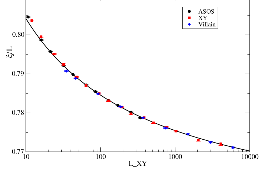
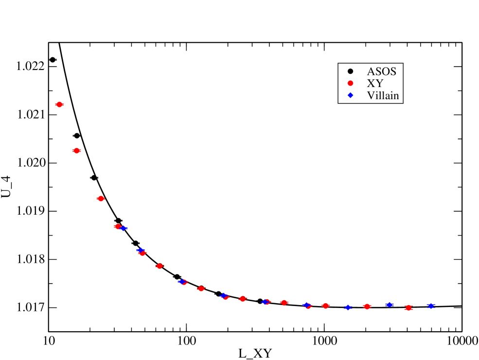
Figure 1: Data for the dual of the ASOS model, the XY model and the Villain model at the KT transition. (See eqs. (11)) In the upper figure we plot $\xi/L$ as a function of the lattice size $L_{XY}$ of the XY model. Following eqs. (11), the lattice size of the dual of the ASOS model and the Villain model are rescaled as $L_{XY}=0.3345\times L_{ASOS}$ and $L_{XY}=2.906\times L_{villain}$. The solid lines give $\xi/L$ and $U_{4}$ obtained from eqs. (6).

Finally, let us discuss the behaviour of the Binder cumulant at the KT-transition. Taking e.g. the result of the fit for the dual of the ASOS model for $L_{min}=96$ and $\tilde{\beta}=0.80608$ one obtains that the minimum of the Binder cumulant at the transition is $U_{4,min}\approx 1.017006$ at $L\approx 6200$. To see the Binder cumulant increase again, rather large lattice sizes are needed: To get a value $1.01701$ we have to go up to $L\approx 11000$ and $1.01705$ is reached at about $L=38000$. I.e. it is impossible with todays computing resources to see explicitly from Monte Carlo simulations that the Binder cumulant at the KT-transition is an increasing function of $L$ for sufficiently large $L$.

6 The matching method

The RG-flow in the neighbourhood of the KT-transition is given, up to irrelevant scaling fields, in terms of two coupling constants, $x=\pi\beta_{SW}-2$ and the fugacity $z$ [3, 4]. Therefore, in finite size scaling we can map the KT-flow using two different phenomenological couplings $R_{1}(x(L),z(L))$ and $R_{2}(x(L),z(L))$. In the ideal case,

$$R_{1}(x,z) = R_{1}(0,0)+c_{1}x+\mbox{O}(z^{2},xz)$$ (43)

$$R_{2}(x,z) = R_{2}(0,0)+c_{2}z+\mbox{O}(x^{2},xz)\;.$$ (44)

In the SOS representation, such pairs of phenomenological couplings can be easily found [13, 14]. In the XY representation, on a finite lattice with periodic boundary conditions vortices come in pairs. Therefore only phenomenological couplings of the type (43) can be constructed.

Since both the helicity modulus $\Upsilon$ and the second moment correlation length over the lattice size $\xi/L$ can be well fitted by eqs. (23,24) it is very hard numerically to observe any explicit $z$-dependence of these quantities. Therefore it is actually fortunate that the Binder cumulant displays a $z^{2}$ contribution with an apparently large amplitude.

Therefore we can at least map the RG-flow in an intermediate regime of lattice sizes using $\xi/L$ or $\Upsilon$ as first phenomenological coupling and $U_{4}$ as second phenomenological coupling. Here, an intermediate regime of lattice sizes means that $L$ should be large enough such that power law corrections due to irrelevant scaling fields can be ignored and on the other hand $L$ is still small enough such that $z^{2}$-contributions in the numerical data of $U_{4}$ are much larger than the statistical error.

The purpose of this mapping is to allow for an accurate determination of $\beta_{KT}$ from relatively small lattices. This can be achieved by solving the following set of equations:

$$R_{1,NM}(L,\beta_{KT,NM}) = R_{1,SM}(\tilde{b}_{m}L,\beta_{KT,SM})$$

$$R_{2,NM}(L,\beta_{KT,NM}) = R_{2,SM}(\tilde{b}_{m}L,\beta_{KT,SM})\;\;,$$ (45)

where $NM$ stands for new model, where $\beta_{KT,NM}$ is not known and $SM$ stands for solved model. In the case of the solved model, $\beta_{KT}$ should be at least determined numerically to a high precision and also the phenomenological couplings should be determined accurately. The unknowns of the eqs. (6) are $\beta_{KT,NM}$ of the new model and the matching factor $\tilde{b}_{m}$.

The right sides of eqs. (6) might be given by the results of our simulations discussed in the previous section. These results could be represented by tables. To obtain values of the phenomenological couplings for any lattice size $L_{min}\leq L\leq L_{max}$, where $L_{min}$ and $L_{max}$ are the minimal and maximal lattice size that are simulated, one might e.g. interpolate the values contained in the table in linearly $\ln(L)$.

Here instead we follow an approach that is simpler to implement. As we have seen in the previous section, our numerical data for $\xi/L$ and $U_{4}$ are well described by the ansätze (41,42). Therefore we suggest to use these, along with the results for the parameters, as right side of eqs. (6). Since in ref. [13, 14] the transition temperature is most accurately determined for the dual of the ASOS model, we use the data of this model for the matching.

In particular we take the result obtained from $L_{min}=96$ at

$$\tilde{\beta}=0.80608 :$$

$$U_{4,ASOS}(L) = 1.018192-\frac{0.017922}{\ln L-1.18}+\frac{0.06769}{(\ln L-1.18)^{2}}$$

$$\frac{\xi_{2nd,ASOS}(L)}{L} = 0.7506912+\frac{0.212430}{\ln L+0.573}\;.$$ (46)

For consistency we also take $\xi/L$ at $\tilde{\beta}=0.80608$ and $L_{min}=96$. Note that in the present context, it is only important that the equation describes the data well for a certain range of lattice sizes ($96\leq L\leq 1024$), where the matching takes place.

To check the error due to the uncertainty of $\tilde{\beta}_{KT}$ one should repeat the matching with the results obtained at

$$\tilde{\beta}=0.80606 :$$

$$U_{4,ASOS}(L) = 1.018192-\frac{0.017922}{\ln L-1.193}+\frac{0.06730}{(\ln L-1.193)^{2}}$$

$$\frac{\xi_{2nd,ASOS}(L)}{L} = 0.7506912+\frac{0.212430}{\ln L+0.557}\;.$$ (47)

Here we do not quote statistical errors and covariances of $C$ for $\xi/L$ and $c_{2}$ and $C$ for $U_{4}$. Note that applying the matching with eqs. (6,6) it makes no sense to produce larger statistics for the new model than the one for the ASOS model here. Staying well below our present statistics, say $10^{6}$ or less measurements for the new model, the statistical error of the coefficients in eqs. (6,6) can be safely ignored. Since we are aiming at models that are harder to simulate than the models discussed in the present work, this is no serious limitation.

7 A first application: the $\phi^{4}$ model at $\lambda=2.1$

We have tested the new method at the example of the 2-component $\phi^{4}$ model on the square lattice. The classical Hamiltonian is given by

$$H_{\phi^{4}}=-\beta\sum_{x,\mu}\vec{\phi}_{x}\cdot\vec{\phi}_{x+\hat{\mu}}+\sum_{x}\left[\vec{\phi}_{x}^{\;2}+\lambda(\vec{\phi}_{x}^{\;2}-1)^{2}\right]\;\;,$$ (48)

where the field variable $\vec{\phi}_{x}$ is a vector with two real components. In our convention, the Boltzmann factor is given by $\exp(-H_{\phi^{4}})$. Since $|\vec{\phi}_{x}|$ is not restricted to one, the model can not be mapped into an SOS model. For our test we have chosen the value $\lambda=2.1$, which is a good approximation of the improved value of the three dimensional model [23]. In the two dimensional case this value has no particular meaning.

We have simulated the model with a mixture of the single cluster algorithm, the overrelaxation update and a local Metropolis update. Here the local Metropolis update is needed to change $|\vec{\phi}_{x}|$. The single cluster algorithm, and the overrelaxation update have exactly the same form as in the case of the XY model. The proposal for the Metropolis update is given by

$$\phi_{x}^{(1)^{\prime}} = \phi_{x}^{(1)}+s\left(r-\frac{1}{2}\right)$$

$$\phi_{x}^{(2)^{\prime}} = \frac{3}{4}\beta\Phi_{x}^{(2)}-\phi_{x}^{(2)}$$ (49)

with $s=3$. $r$ is a random number with a uniform distribution in the interval $[0,1]$. ${\Phi_{x}}$ is the sum over the nearest neighbours of $x$. The proposal for the second component of the field is constructed such that $H_{\phi^{4}}$ is only changed by little. The proposal is accepted with the probability $A=\mbox{min}[1,\exp(-\Delta H)]$. This Metropolis update is followed by a second update at the same site, where the role of the two components of the field is exchanged. These updates were performed the following sequence: One Metropolis sweep, one sweep with the overrelaxation algorithm, 10 single cluster updates, followed by 5 sweeps with the overrelaxation algorithm. After such a sequence of updates, a measurement of the observables is performed.

We have simulated $L=32$ at $\beta=1.075$ and $1.08$, $L=64$ at $\beta=1.078$ and $1.08$, $L=128$ at $\beta=1.077$ and $\beta=1.079$ and $L=256$ at $\beta=1.0775$ and $\beta=1.0785$. In all cases we have performed $10^{7}$ measurements. For fitting the data with the ansätze (40,41) and for the matching (6), we linearly interpolated the values of $\Upsilon$, $\xi/L$ and $U_{4}$ in $\beta$.

First we have fitted the helicity modulus to the ansatz (40), where $\beta_{KT}$ and the integration constant $C$ are the free parameters. The results of these fits are summarized in table 9. $\chi^{2}/$d.o.f. is quite large and the result for $\beta_{KT}$ is decreasing with increasing $L_{min}$.

Table 9: Fitting $\Upsilon$ of the $\phi^{4}$ model at $\lambda=2.1$ with the analogue of the ansatz (40).

$L_{min}$	$\beta_{KT}$	$C$	$\chi^{2}/$d.o.f.
32	1.07865(1)	0.278(2)	75.9
64	1.07838(2)	0.363(7)	22.6
128	1.07818(2)	0.447(8)	-

Next we have fitted the data for $\xi/L$ to the ansatz (41). The results are summarized in table 10. The $\chi^{2}/$d.o.f. is already smaller than two for $L_{min}=32$. But on the other hand also the statistical error of $\beta_{KT}$ obtained from $\xi/L$ is about 6 times larger than for that from the helicity modulus. In the case $\xi/L$ the estimate of $\beta_{KT}$ is an increasing function of $L_{min}$. Therefore we might regard the result from $\xi/L$ and $L_{min}=128$ as lower bound and that from $L_{min}=128$ from the helicity modulus as upper bound. Hence we quote $\beta_{KT}=1.0779(5)$ as our final estimate obtained from the combined analysis of $\Upsilon$ and $\xi/L$.

Table 10: Fitting $\xi/L$ of the $\phi^{4}$ model at $\lambda=2.1$ with the analogue of the ansatz (41).

$L_{min}$	$\beta_{KT}$	$C$	$\chi^{2}/$d.o.f.
32	1.07721(6)	1.50(2)	1.67
64	1.07739(12)	1.41(6)	1.39
128	1.07761(19)	1.30(9)	-

Next we applied the matching method discussed in the previous section.

Table 11: Matching the $\phi^{4}$ model at $\lambda=2.1$ with the dual of the ASOS model at $\beta=0.80608$, eqs. (6).

$L$	$L_{ASOS}$	$\beta_{KT}$
32	55.81(12)	1.07892(4)
64	113.6(5)	1.07822(3)
128	234.2(1.4)	1.07786(2)
256	479.(5.)	1.07776(2)

Table 12: Matching the $\phi^{4}$ model at $\lambda=2.1$ with the dual of the ASOS model at $\beta=0.80606$, eqs. (6).

$L$	$L_{ASOS}$	$\beta_{KT}$
32	56.03(12)	1.07898(4)
64	113.8(5)	1.07827(3)
128	234.0(1.4)	1.07790(2)
256	478.(5.)	1.07780(2)

This way we obtain an estimate of $\beta_{KT}$ and the corresponding lattice size of the ASOS model from a single lattice size $L$. Our results for matching with $\beta_{ASOS}=0.80608$, eqs.(6), are given in table 11 and those for $\beta_{ASOS}=0.80606$, eqs.(6), in table 12. The estimates for $\beta_{KT}$ apparently converge as $L$ increases. Taking into account the difference between $L=128$ and $L=256$ as well as the difference between $\beta_{ASOS}=0.80608$ and $\beta_{ASOS}=0.80606$ we arrive at our final estimate $\beta_{K}T=1.0778(2)$. This estimate is clearly more precise than that obtained from fitting $\Upsilon$ and $\xi/L$ with the ansätze (40,41).

8 Summary and Conclusions

We have studied the XY model, the Villain model and the dual of the absolute value solid-on-solid model on a square lattice at the Kosterlitz-Thouless transition. We have focused on the behaviour of phenomenological couplings like the helicity modulus $\Upsilon$, the second moment correlation length over the lattice size $\xi/L$ and in particular the Binder cumulant $U_{4}$.

Using Monte Carlo simulations of the Gaussian model on the square lattice, we have determined the asymptotic value of $U_{4}$ and the leading logarithmic correction at the Kosterlitz-Thouless transition. See eq. (34).

We confronted the predictions (23,24,34) for the phenomenological couplings derived from the Kosterlitz-Thouless theory with the results of our Monte Carlo simulations. We have reached lattice sizes of $L=4096$, $2048$ and $1024$ for the XY model, the Villain model and the dual of the ASOS model, respectively. We have generated several $10^{6}$ statistically independent configurations for each lattice size.

We find that the data for the helicity modulus $\Upsilon$ and in particular the second moment correlation length over the lattice size $\xi/L$ follow quite well the predictions (23,24).

In contrast, the value of the Binder cumulant at the KT-transition is increasing with increasing lattice size, while eq. (34) predicts that the Binder cumulant should decrease for sufficiently large lattice sizes. This discrepancy is explained by the presence of vortex pairs that have a distance of order $L/2$. This effect should be proportional to the fugacity squared. Hence it should lead to a subleading correction. Indeed adding a term $c_{2}/(\ln L+C)^{2}$ to the ansatz allows to fit our data for the Binder cumulant for all three models studied. The values for $c_{2}$ obtained for the three models are consistent, confirming the universal character of the subleading correction. From the results of these fits one can easily see that with the present computer resources it is not possible to reach sufficiently large lattices with high statistics to see explicitly the asymptotic behaviour of the Binder cumulant (34).

The fact that $U_{4}$ behaves quite differently from $\xi/L$ and $\Upsilon$ allows us to set up a matching method similar to that of ref. [13, 14] for solid-on-solid models. For a detailed discussion see section 6.

As a first test, we have applied the matching method to the two component $\phi^{4}$ model on the square lattice at $\lambda=2.1$. We find that using moderately large lattices (up to $L=256$), we can determine the temperature of the KT-transition quite accurately. We show that the new matching method is superiour to fits of $\Upsilon$ or $\xi/L$ to the predictions (23,24).

In the near future we plan to apply the method to thin films of the three dimensional two component $\phi^{4}$ model and the dynamically diluted XY model, where the duality transformation to solid-on-solid models is not available.

9 Acknowledgement

I like to thank I. Campbell for pointing my attention to ref. [10].

References

- [1] J.M. Kosterlitz and D.J. Thouless, J. Phys. C 6 (1973) 1181; J.M. Kosterlitz, J. Phys. C 7 (1974) 1046.
- [2] N.D. Mermin and H. Wagner, Phys. Rev. Lett. 17 (1966) 1133.
- [3] J.V. José, L.P. Kadanoff, S. Kirkpatrick and D.R. Nelson, Phys. Rev. B 16 (1977) 1217.
- [4] D.J. Amit, Y.Y. Goldschmidt and G. Grinstein, J. Phys. A 13 (1980) 585.
- [5] E.H. Lieb, Phys. Rev. 162 (1967) 162.
- [6] E.H. Lieb and F.Y. Wu, in: ‘Phase Transitions and Critical Phenomena’, C. Domb and N.S. Green, eds., Vol. 1, Academic, 1972.
- [7] R.J. Baxter, ‘Exactly Solved Models in Statistical Mechanics’, Academic Press, 1982.
- [8] H. van Beijeren, Phys. Rev. Lett. 38 (1977) 993.
- [9] D. Loison , J. Phys. C 11 (1999) L401.
- [10] G.M. Wysin and A.R, Pereira, I.A. Marques, S.A. Leonel, and P.Z. Coura, Phys. Rev. B 72 (2005) 094418, [arXiv:cond-mat/0504145].
- [11] R. Savit, Rev. Mod. Phys. 52 (1980) 453.
- [12] T. Korzek, Comparison of exact and numerical results in the XY model, Diploma thesis, Humboldt Universität zu Berlin 2003.
- [13] M. Hasenbusch, M. Marcu and K. Pinn, Physica A 208 (1994) 124 [arXiv:hep-lat/9404016].
- [14] M. Hasenbusch and K. Pinn, J. Phys. A 30 (1997) 63 [arXiv:cond-mat/9605019].
- [15] M.E. Fisher, M.N. Barber and D. Jasnow, Phys. Rev. A 8 (1973) 1111.
- [16] S. Teitel and C. Jayaprakash, Phys. Rev. B 27 (1983) 598; Y.-H. Li and S. Teitel, Phys. Rev. B 40 (1989) 9122.
- [17] M. Le Bellac, ‘Quantum and Statistical Field Theory’, Oxford University Press (1991).
- [18] M. Hasenbusch, J. Phys. A: Math. Gen. 38 (2005) 5869 [arXiv:cond-mat/0502556].
- [19] H. Weber and P. Minnhagen, Phys. Rev. B 37 (1988) 5986.
- [20] U. Wolff, Phys. Rev. Lett. 62 (1989) 361.
- [21] H.G. Evertz, M. Hasenbusch, M. Marcu, K. Pinn and S. Solomon, Phys.Lett. B 254 (1991) 185.
-
[22]
M. Saito, An Application of Finite Field: Design and Implementation of
128-bit Instruction Based Fast Pseudorandom Number Generator,
Master Thesis, Dept. of Math., Graduate School of Science
Hiroshima University 2007;
www.math.sci.hiroshima-u.ac.jp/m-mat/MT/SFMT/index.html - [23] M. Campostrini, M. Hasenbusch, A. Pelissetto and E. Vicari, Phys. Rev. B 74 (2006) 144506 [arXiv:cond-mat/0605083].