Light curve and neutrino spectrum emitted during the collapse of a nonrotating, supermassive star.

Abstract

The formation of a neutrino pulse emitted during the relativistic collapse of a spherical supermassive star is considered. The free collapse of a body with uniform density in the absence of rotation and with the free escape of the emitted neutrinos can be solved analytically by quadrature. The light curve of the collapsing star and the spectrum of the emitted neutrinos at various times are calculated.

1 INTRODUCTION

The properties of a neutrino pulse arising during the spherically symmetrical collapse of a supermassive star into a black hole have been considered in a number of studies, the earliest of which were carried out nearly 40 years ago [1]. It was shown in [2] that, in general, the asymptotic time dependence of the total luminosity of the star has the form

$$I\propto\exp\displaystyle{\left(-\frac{ct}{3\sqrt{3}r_{g}}\right)}$$

The propagation of photons outside a nonrotating collapsing star was considered in detail in [3]. The brightness distribution across the visible disk and the time dependence of the stellar spectrum were obtained for late stages of the collapse. The results of numerical computations of the light curve and the spectrum of a nonrotating, collapsing star are presented by Shapiro [4, 5], who computed the propagation of photons inside the star in a diffusion approximation taking into account general relativistic effects. The propagation of photons to a distant observer is also treated in detail in [4]. Estimates of the parameters of the spectrum and of the total intensity of a neutrino pulse arising during the collapse of a supermassive state were obtained in [6]. The possibility of detecting such a pulse using modern detectors was analyzed, and the general background of neutrinos arising as a result of explosions of supermassive stars was estimated. The results of relativistic hydrodynamical computations of the collapse of a nonrotating, supermassive star are presented in [7], together with temperature and density profiles for the matter inside the star at various times. However, the propagation of the neutrinos was computed using a very simple scheme; it was essentially assumed that the neutrinos propagated instantaneously. In addition, all general relativistic effects were neglected.

Thus, in spite of the abundance of publications on the topic, the properties of neutrino pulses arising during the collapse of supermassive stars are not fully understood. As a rule, previous papers have either considered very simple models for this phenomenon that have admitted exact solutions (as in [1]), constructed very detailed models that have required the use of approximation computational methods, or have neglected certain physically important effects. For example, the propagation of the neutrinos is taken to be instantaneous in [7], and gravitational forces are not taken into account. Such an approach is clearly not justified physically. During the collapse of a supermassive star, the temperature of the matter grows as the collapse proceeds; accordingly, the neutrinoloss rate in a comoving frame also grows, reaching its highest values in the late stages of the collapse. The drop in the radiation intensity at the end of the collapse is due exclusively to gravitational effects: the gravitational redshift and time dilation. Thus, the shape of the light curve is determined by the battle between two competing processes: the increase in the brightness of the star due to heating and the decrease in its brightness due to gravitational effects. In addition, the characteristic time scale for the collapse $\displaystyle{\frac{r_{g}}{c}}$ is comparable to the time for a neutrino to travel a distance equal to the radius of the star. Under such conditions, the neglect of gravitational effects and of the neutrino-propagation time is completely unjustified. Ordinary (not supermassive) stars were considered in [5]; these computations included all general relativistic effects, but the propagation of the neutrinos inside the star was treated in an Eddington approximation, which cannot be formulated unambiguously inside the star, where the effects of sphericity are appreciable.

The aim of the current paper is to construct a model for the neutrino emission radiated by a supermassive star that can yield as accurate a solution as possible, including all general relativistic effects, while simultaneously providing a good description of a real collapsing star. The light curve and spectra obtained with this model should display all the main properties characteristic of the light curves and spectra of real collapsing supermassive stars, while the simplicity of the model enables us to understand the dependence of the parameters of the neutrino impulse on the parameters of the problem. As we will show below, by introducing a number of natural constraints on the parameters of the problem, we can obtain a solution by quadrature.

2 DYNAMICS OF THE COLLAPSE

We introduce a number of assumptions about the physical parameters of the collapse that simplify the computations. Most importantly, the star is taken to be nonrotating and the distribution of matter to be uniform at all times. In addition, we neglect completely the influence of the pressure on the motion of the matter; i.e., the dynamics of the collapse are taken to be the same as for a sphere of dust. We also assume that the matter is heated according to a power law as a result of compression. Our neglect of the pressure is a rather crude approximation at the onset of the collapse, but the temperature of the matter is still modest at this stage, and few neutrinos are radiated. As the star approaches its gravitational radius $r_{g}$, the influence of the pressure tends to zero, so that it indeed becomes negligible. As is shown in [8], inside a homogeneous dust sphere that is shrinking or expanding, it is possible to introduce a comoving, synchronous coordinate system in which ordinary three-dimensional space has the same curvature everywhere, which depends only on time. The character of this curvature (positive, negative, zero) does not change in the course of the collapse and is uniquely specified by the initial conditions (initial density and velocity). We will take the three-dimensional space inside the sphere to have zero curvature, which appreciably simplifies the computations without introducing large errors.

Let the initial radius of the star be $x_{0}$. According to [8], the metric inside the dust sphere can be written as

$$ds^{2}=d\tau^{2}-a^{2}(\tau)[dR^{2}+R^{2}(d\zeta^{2}+\sin^{2}\!\zeta\;d\xi^{2})]$$ (1)

$$\mbox{where}\quad a(\tau)=\left(1-\frac{\tau}{\tau_{col}}\right)^{\frac{2}{3}}$$ (2)

Here $\tau_{col}$, is a parameter of the problem that is defined below and the ”spatial” coordinates ($R,\zeta,\xi$) are analogous to the usual spherical coordinates in threedimensional space.T he coefficient $a$ plays the role of a scale factor: to find the physical distance between two points in the metric (1), we must multiply the ”coordinate distance” [calculated in the coordinates ($R,\zeta,\xi$)) by $a$. In particular, the distance from a point with radial coordinate $R$ to the center of the star is:

$$x=aR$$ (3)

The coordinate system ($\tau,R,\zeta,\xi$) is comoving. This means that each element of the collapsing matter has some fixed $R,\zeta$ and $\xi$ that do not change in time. In this sense, ($R,\zeta,\xi$) can be considered Lagrange coordinates.

Note the full analogy between the solution for a collapsing dust sphere considered here and the Friedmann solution for a flat universe filled with homogeneous dust, whose metric coincides fully with 1. Therefore, the inner space of the dust sphere can be considered part of a Friedmann universe; the motion of the neutrinos within the dust sphere occurs precisely as within a Friedmann universe. In a comoving coordinate system, the radial coordinate $R_{s}$ of the surface does not change and at any time $\tau<\tau_{col}$ is equal to its initial value

$$R_{s}=\frac{x_{s}}{a}=R_{s0}=\frac{x_{s0}}{a_{0}}$$ (4)

In addition, it is straightforward to obtain the following relation using the results of [8]:

$$2\pi k\varepsilon=\frac{1}{3\tau^{2}_{col}a^{3}}$$ (5)

Here, $k$ is the gravitational constant and $\varepsilon$ is the density of the stellar matter in its rest frame.Integrating $\varepsilon$ over the entire volume of the collapsing sphere yields the total rest mass of the stellar matter. It is of interest to determine how this quantity is related to the total mass of the star measured by a distant stationary observer. This latter mass consists of the rest mass of the matter and the sum of its kinetic and potential energy. As was noted above, we are considering the collapse of a dust sphere within which the three-dimensional curvature of space is zero. In this case, the motion of dust matter toward the center is a free fall with zero velocity at infinity. The sum of the kinetic and potential energy of matter undergoing such a free fall is zero. Therefore, the mass of the star is equal to the rest mass of its matter, i.e.,

$$M=\int\varepsilon dV$$ (6)

Hence, taking into account also the homogeneity of the star, we have

$$\varepsilon=\frac{3M}{4\pi x^{3}_{s}}$$ (7)

Combining this relation with (5) yields

$$\frac{3kM}{2x^{3}_{s}}=\frac{1}{3\tau^{2}_{col}a^{3}},\quad\mbox{in other words, in accordance with (\ref{a3})}\quad kM=\frac{2R^{3}_{s}}{9\tau^{2}_{col}}.$$ (8)

Since in our units $r_{g}=c=1$, it follows from the definition $r_{g}=\frac{2kM}{c^{2}}$ that

$$kM=\frac{1}{2}$$ (9)

which yields

$$\frac{4R^{3}_{s}}{9\tau^{2}_{col}}=1,\qquad\tau_{col}=\frac{2}{3}R^{\frac{3}{2}}_{s}$$ (10)

We will adopt the time $\tau=0$ as the initial time. Then, $a_{0}=1$ and

$$x_{s0}=R_{s0}=R_{s}.$$ (11)

Having specified the initial radius of the star $x_{s0}$, we can use (10) to determine the collapse parameter $\tau_{col}$. The collapse of a uniform sphere with a flat internal space involves two independent parameters: the Lagrange radius of the surface $R_{s}$ and the mass of the star. The quantity $\tau_{col}-\tau_{0}$ is uniquely determined by these two parameters, and variations in $\tau_{0}$ only shift the zero time. In the case of arbitrary three-dimensional curvature, we can arbitrarily specify the mass, initial radius, and initial collapse velocity of the star. If we consider a collapse with zero curvature, this is not possible, and the initial collapse velocity always differs from zero for a finite initial radius. This is automatically determined from the condition of zero curvature and turns out to be equal to the velocity for free fall from infinity for the radius $x_{s0}$. In the interest of conciseness, we will denote the initial radius of the star simply as $x_{0}$.

3 COMPUTATION OF THE RADIATION SPECTRUM IN A COMOVING FRAME

We will assume that each matter element emits neutrinos isotropically in a comoving frame and that the intensity and spectrum of the emitted neutrinos depend on the temperature and density of the matter. In our analysis, the dynamics of the collapse corresponds to the motion of the dustlike material. If the law for variations of the density and the parameters $M$ and $R_{s}$ is known, the variations of the temperature in the compressed matter can be found from the solution of the energy equation for a specified initial entropy using the known rate of neutrino emission as a function of the temperature and density. Below, we use a simplified approach in order to obtain an analytical solution, in which we approximate the time dependence of the temperature with a power-law dependence of the temperature on the density. The variations of the density of the matter $\varepsilon(\tau)$ are determined in accordance with (4) and (7) by the single function $a(\tau)$. To find the observed light curve and spectrum of the neutrinos, we must first determine the propagation toward the observer of a neutrino signal arising within a uniform collapsing body of a specified mass $M$.

We will suppose that

$$f(a,q)dVd^{3}pd\tau$$ (12)

neutrinos are emitted in an element of physical volume $dV$ in an element of physical phase space $d^{3}p$ in an interval of proper time $d\tau$ in the element’s rest frame, where $f(a,q)$ is some function whose form will be determined below.

We introduce the neutrino distribution function $N$ such that the quantity $Nd^{3}pdV$ specifies the number of neutrinos in an element of physical volume $dV$ in an element of physical phase space $d^{3}p$. In the spherically symmetric case with isotropic neutrino emission in the comoving frame, $N$ depends on only four quantities: the radial coordinate $R$, the angle between the neutrino trajectory and the direction from the center of the star $\vartheta$, the neutrino energy $q$, and time $\tau$. In this case, the kinetic equation can be written in the form [9]

$$\cos\vartheta\frac{\partial N}{\partial R}-\frac{\sin\vartheta}{R}\frac{\partial N}{\partial\vartheta}+\frac{2q}{3\tau_{col}\sqrt{a}}\frac{\partial N}{\partial q}-\frac{2\sqrt{a}}{3\tau_{col}}\frac{\partial N}{\partial a}=af(a,q)$$ (13)

Here, the parameter $a$, which depends on time in accordance with (2), is used in place of the time $\tau$. The characteristic system for this equation has the form

$$\frac{dR}{\cos\vartheta}=dy$$ (14)

$$-\frac{Rd\vartheta}{\sin\vartheta}=dy$$ (15)

$$\frac{3\tau_{col}\sqrt{a}dq}{2q}=dy$$ (16)

$$-\frac{3\tau_{col}da}{2\sqrt{a}}=dy$$ (17)

The solutions of this system determine the trajectories of individual neutrinos.Combining pairwise the equations for characteristic system (16) and (17), and also (14) and (15), we obtain the two first integrals:

$$A=aq$$ (18)

$$B=R\sin\vartheta$$ (19)

Combining (15) and (17) and using (19), we obtain the third, last, integral of the system (14)-(17).

$$C=3\tau_{col}\sqrt{a}+R\cos\vartheta$$ (20)

The physical meaning of these quantities can be elucidated based on the analogy between the solution for a collapsing dust sphere and the solution for a Friedmann universe. As was noted above, the motion of a neutrino is absolutely identical in these two cases; in particular, all three of the first integrals of system (14)-(17) are also valid in a Friedmann universe. The presence of integral (18), i.e., the fact that the product $a\cdot q$ is constant, leads to the appearance of a ”redshift” in a Friedmann universe. As the parameter $a$ increases (corresponding to the expansion of space), the energy of a neutrino along its trajectory decreases. In contrast, in our case we have a compression of a sphere, so that $a$ decreases and the neutrino energy increases. Thus, we can think of our case as giving rise to a ”violet shift”.

Supermassive stars with masses exceeding $\sim 10^{5}M_{\odot}$ have small optical depths to the absorption of neutrinos, which can be taken to propagate freely. Taking the radius of the star to be $R=nR_{g}=2nGM/c^{2}$, we obtain expressions for the mean density,

$$\rho=\frac{3M}{4\pi R^{3}}=\frac{1.8\cdot 10^{16}}{n^{3}}\left(\frac{M_{\odot}}{M}\right)g/cm^{3}$$

and the optical depth to neutrino absorption,

$$\tau_{\nu}=10^{-44}\rho R=\frac{33}{n^{2}}\frac{M_{\odot}}{M}\ll 1$$

for $n\simeq 3$, $M=10^{5}M_{\odot}$.

Let us elucidate the qualitative form of the characteristics determining system (14)-(17). The motion of photons and neutrinos is linear in a Friedmann universe. Indeed, integral (19) shows that a neutrino moves along straight lines in the ($\tau,R,\zeta,\xi$) coordinate frame. In addition, since this frame is comoving, the collapsing star can be represented at any time in this frame as a sphere with a constant radius $R_{s}$. The trajectory described by (14)-(17) proves to be a chord of this sphere. In accordance with the definition of the angle $\theta$, the trajectory enters the sphere at some angle $\vartheta>\frac{\pi}{2}$ and leaves at an angle $\vartheta<\frac{\pi}{2}$. Proceeding from this property of the characteristic, it is straightforward to impose the appropriate boundary conditions for (13). For this, it is sufficient to specify the value of the function $N$ at the surface of the star for angles $\vartheta>\frac{\pi}{2}$. We will assume that no neutrinos impact the star from outside, in which case

$$\left.N\right|_{R=R_{s}}=0\quad\mbox{ }\quad\vartheta>\frac{\pi}{2}$$ (21)

This is the boundary condition for (13).

We will denote the initial point of the characteristic and all related quantities with the subscript I and the final point and related quantities with the subscript II. Since both points are located on the surface of the collapsing sphere,

$$R_{I}=R_{II}=R_{s}$$ (22)

Hence, we obtain using (19):

$$\sin\vartheta_{I}=\sin\vartheta_{II}$$ (23)

Since $\vartheta_{I}>\frac{\pi}{2},\vartheta_{II}<\frac{\pi}{2}$,

$$\cos\vartheta_{I}=-\cos\vartheta_{II}$$ (24)

In addition, it follows from the existence of the integral (18) that

$$a_{I}q_{I}=a_{II}q_{II}\quad\mbox{ . .}\quad a_{I}=a_{II}\frac{q_{II}}{q_{I}}$$ (25)

Finally, writing integral (20), we obtain

$$3\tau_{col}\sqrt{a_{I}}+R_{I}\cos\vartheta_{I}=3\tau_{col}\sqrt{a_{II}}+R_{II}\cos\vartheta_{II}$$ (26)

Using relations (24) and (25), we obtain

$$\sqrt{a_{II}\frac{q_{II}}{q_{I}}}=\sqrt{a_{II}}+\frac{2R_{s}}{3\tau_{col}}\cos\vartheta_{II}$$ (27)

$$q_{I}=\frac{q_{II}}{\left(\displaystyle{1+\displaystyle{\frac{2R_{s}}{\displaystyle{3\tau_{col}\sqrt{a_{II}}}}}\cos\vartheta_{II}}\right)^{2}}$$ (28)

Let us turn to the solution of (13) itself. We first take the neutrino-emission function (12) to be

$$f(a,q)=\lambda a^{\beta}\delta(q-q_{0})$$ (29)

i.e., each element of matter in the proper frame radiates monochromatic neutrinos with energy $q_{0}$. Here, $\lambda$ and $\beta$ are numerical parameters. Since (13) is linear, the resulting solution can easily be generalized to the case of a more complex function $f(a,q)$. We will discuss the form of this function for a real system and possible values of the power-law index $\beta$ in more detail below.

For a neutrino-emission function of the form (29), Eq. (13) can be written in the form

$$\cos\vartheta\frac{\partial N}{\partial R}-\frac{\sin\vartheta}{R}\frac{\partial N}{\partial\vartheta}+\frac{2q}{3\tau_{col}\sqrt{a}}\frac{\partial N}{\partial q}-\frac{2\sqrt{a}}{3\tau_{col}}\frac{\partial N}{\partial a}=\lambda a^{\beta+1}\delta(q-q_{0})$$ (30)

To solve this equation, we must integrate the righthand side along the characteristic.Using boundary condition (21), we obtain for the surface of the collapsing sphere:

$$N=\int\limits_{I}^{II}\lambda a^{\beta+1}\delta(q-q_{0})dy$$ (31)

We obtain using (18)-(28)

$$N=\int\limits_{I}^{II}\frac{3}{2}\tau_{col}\lambda\frac{A^{\beta+\frac{3}{2}}}{q^{\beta+\frac{5}{2}}}\delta(q-q_{0})dq=\frac{3}{2}\tau_{col}\lambda\frac{A^{\beta+\frac{3}{2}}}{q_{0}^{\beta+\frac{5}{2}}}\left(\Xi[q_{II}-q_{0}]-\Xi[q_{I}-q_{0}]\right)$$ (32)

Here, the function $\Xi$ is defined to be

$$\Xi[x]=\left\{\begin{array}[]{rcl}0\qquad{\textrm{ }}\qquad x<0,\\ 1\qquad{\textrm{ }}\qquad x>0.\\ \end{array}\right.$$

Note that quantities relating to the end of the characteristic are those that are measured by an observer located on the surface of the collapsing star. Therefore, we can omit the subscript ”II”. Substituting relations (18) and (28) into (32), we finally obtain

$$N=\frac{3}{2}\tau_{col}\lambda\frac{a^{\beta+\frac{3}{2}}q^{\beta+\frac{3}{2}}}{q_{0}^{\beta+\frac{5}{2}}}\left(\Xi[q-q_{0}]-\Xi\biggl{[}q-\left(1+\displaystyle{\frac{2R_{s}}{\displaystyle{3\tau_{col}\sqrt{a}}}}\right)^{2}q_{0}\biggr{]}\right)$$ (33)

This formula specifies the neutrino distribution function measured by an observer located on the surface of the star and moving with this surface.

4 PROPAGATION OF NEUTRINOS FROM THE STAR TO AN OBSERVER

Let us now consider the motion of the neutrinos outside the star.The gravitational field here is a Schwarzschild field [10]; i.e., it has the metric

$$ds^{2}=\left(1-\frac{1}{r}\right)dt^{2}-\left(1-\frac{1}{r}\right)^{-1}dr^{2}-r^{2}(d\theta^{2}+\sin^{2}\!\theta\;d\phi^{2})$$ (34)

The neutrino distribution function $N$ in such a field in the spherically symmetrical case depends on four quantities: the angle between the neutrino trajectory and the direction from the center of the star $\theta$, the neutrino energy $w$, the radius $r$, and the time $t$. We can find N by solving the kinetic equation, for which the boundary conditions must be obtained using (33). Let us determine the relationship between physical quantities measured on the surface of the star in the Friedmann and Schwarzschild reference frames.Loc al observers in the Schwarzschild frame are stationary, while local observers in the Friedmann frame move along with the stellar material. Therefore, physical quantities measured by such observers at some time at the same point on the stellar surface will be related by the usual Lorentz transformation. The velocity in this transformation is the physical velocity of the stellar surface measured by a local Schwarzschild observer, which will be equal to [10]

$$V=\frac{1}{\sqrt{h}}$$ (35)

where $h$ is the current Schwarzschild radius of the star.

The circumference of the stellar surface in the Friedmann frame is $2\pi x$, and in the Schwarzschild frame, $2\pi h$. Since dimensions perpendicular to the motion are not changed by the Lorentz transformation, $2\pi x=2\pi h$, i. e., $x=h$. Thus, the Schwarzschild radius of the star is equal to $x$. In particular, (35) can be rewritten as

$$V=\frac{1}{\sqrt{x}}$$ (36)

As is shown in [8], the physical distribution function of the particles is Lorentz invariant. Therefore, to recalculate function (33) in the Schwarzschild frame, we can simply express the variables $(q,\cos\vartheta)$ in terms of the quantities $(w_{s},\cos\theta_{s})$ in the Schwarzschild frame using the Lorentz transformation and the velocity determined by (36). Using the results of [8], it is straightforward to obtain the relations:

$$q=w_{s}\frac{1+V\cos\theta_{s}}{\sqrt{1-V^{2}}}=w_{s}\frac{\sqrt{x}+\cos\theta_{s}}{\sqrt{x-1}}$$ (37)

$$\cos\vartheta=\frac{\cos\theta_{s}+V}{1+V\cos\theta_{s}}=\frac{\sqrt{x}\cos\theta_{s}+1}{\sqrt{x}+\cos\theta_{s}}$$ (38)

Substituting (37) and (38) into (33), we finally obtain

$$\left.N\right|_{r=x}=\frac{\lambda}{x^{\beta}_{0}}\frac{x^{\beta+\frac{3}{2}}}{q^{\beta+\frac{5}{2}}_{0}}\left(w_{s}\frac{\sqrt{x}+\cos\theta_{s}}{\sqrt{x-1}}\right)^{\beta+\frac{3}{2}}\times$$

$$\left(\Xi\left[w_{s}-\left(\frac{\sqrt{x-1}}{\sqrt{x}+\cos\theta_{s}}\right)q_{0}\right]-\Xi\left[w_{s}-\left(\frac{\sqrt{x-1}}{\sqrt{x}+\cos\theta_{s}}\right)\left(1+\frac{\sqrt{x}\cos\theta_{s}+1}{\sqrt{x}\cos\theta_{s}+x}\right)^{2}q_{0}\right]\right)$$ (39)

Thus, we have derived the physical neutrino distribution function on the stellar surface in the Schwarzschild frame.T o fully specify the boundary conditions, we must determine an expression describing the motion of this surface.T he equation for radial free fall of a body in a Schwarzschild field is such that the velocity of the body is zero at infinity [10] (as was indicated above, the surface of the dust sphere moves in precisely this way) and has the form

$$t=\ln\left(\frac{\sqrt{x}+1}{\sqrt{x}-1}\right)-\frac{2}{3}x^{\frac{3}{2}}-\sqrt{x}+D$$ (40)

Here, $D$ is the constant of integration.By specifying this constant, we determine the zero time in the Schwarzschild frame. Setting $D$ equal to zero, we obtain

$$t=\ln\left(\frac{\sqrt{x}+1}{\sqrt{x}-1}\right)-\frac{2}{3}x^{\frac{3}{2}}-\sqrt{x}$$ (41)

This formula describes the motion of the stellar surface. Thus, we have fully specified the boundary conditions for the kinetic equation in the Schwarzschild metric.The kinetic equation for such a field was obtained in [2], where it was shown that, in this case, the integrals of motion have the form

$$\rho=\frac{r\sqrt{r}}{\sqrt{r-1}}\sin\theta$$ (42)

$$\Omega=w\left(1-\frac{1}{r}\right)^{\frac{1}{2}}$$ (43)

$$\xi=t-\int\limits_{x(\xi)}^{r}\frac{z^{2}\sqrt{z}}{(z-1)\sqrt{z^{3}-\rho^{2}(z-1)}}\,dz$$ (44)

The first of these quantities specifies the impact parameter in the Schwarzschild field, and the second determines the redshift for the motion of a neutrino in such a field. The third integral is essentially the time when the neutrino is emitted from the stellar surface. However, it will be more convenient for us to use in place of the time when the neutrino is emitted, $\xi$, the radius of the star at this time, $x$. It is obvious that these quantities are unambiguously related to each other in accordance with (41):

$$\xi=\ln\left(\frac{\sqrt{x}+1}{\sqrt{x}-1}\right)-\frac{2}{3}x^{\frac{3}{2}}-\sqrt{x}$$ (45)

Let us now express the quantities $\cos\theta_{s}$ and $w_{s}$ in (39) in terms of the integrals of motion $\Omega$, $\rho$ and $x$. We substitute the values of variables corresponding to the stellar surface into formulas (42)-(44) (in particular, we must set $r=x$). This yields

$$\rho=\frac{x\sqrt{x}}{\sqrt{x-1}}\sin\theta_{s}$$ (46)

$$\Omega=w_{s}\left(1-\frac{1}{x}\right)^{\frac{1}{2}}$$ (47)

Hence,

$$w_{s}=\sqrt{\displaystyle{\frac{x}{x-1}}}\Omega$$ (48)

$$\cos\theta_{s}=\frac{\sqrt{x^{3}-\rho^{2}(x-1)}}{x\sqrt{x}}$$ (49)

Substituting the resulting expressions into formula (39) for the neutrino distribution function at the stellar surface,

$$N=\frac{2\lambda}{x^{\beta}_{0}}\frac{x^{\beta+\frac{3}{2}}\Omega^{\beta+\frac{3}{2}}}{q^{\beta+\frac{5}{2}}_{0}m^{\beta+\frac{3}{2}}}\left(\Xi\left[\Omega-mq_{0}\right]-\Xi\left[\Omega-g^{2}mq_{0}\right]\right)$$ (50)

Here, we have introduced the notation

$$u=\sqrt{x^{3}-\rho^{2}(x-1)};\quad m=\frac{x(x-1)}{x^{2}+u};\quad\displaystyle{g=1+\frac{x+u}{x^{2}+u}}$$ (51)

Since the space outside the star does not contain any neutrino sources, the the distribution function is constant along the characteristics. Therefore, the resulting expression specifies the neutrino distribution at an arbitrary point outside the star.

However, we are ultimately interested in the parameters of a neutrino pulse that is measured by an observer infinitely distant from the collapsing star. Let the distance from the observer to the star be $d$ $(d\gg 1)$. Thus, we will be interested in the behavior of the integrals (42)-(44) for $r=d$, i. e., $r\gg 1$. The first two integrals, ((42) and (43)), acquire the form

$$\rho=d\sin\theta$$ (52)

$$\Omega=w$$ (53)

As is noted above, we use $x$ in place of the integral $\xi$ from system (42)-(44); these quantities are unambiguously related by (45). We substitute this relation into (44) and express the time $t$ when the neutrino reaches the radius $r$ in terms of $x$ and $\rho$.

$$t=\ln\left(\frac{\sqrt{x}+1}{\sqrt{x}-1}\right)-\frac{2}{3}x^{\frac{3}{2}}-2\sqrt{x}+\int\limits_{x}^{r}\frac{z^{2}\sqrt{z}}{(z-1)\sqrt{z^{3}-\rho^{2}(z-1)}}\,dz$$ (54)

We transform the integral in this formula by substituting $r$ with $d$.

$$\int\limits_{x}^{d}\frac{z^{2}\sqrt{z}}{(z-1)\sqrt{z^{3}-\rho^{2}(z-1)}}\,dz=d+\ln(d-1)-x-\ln(x-1)+$$

$$+\int\limits_{x}^{d}\frac{z}{z-1}\left[\frac{z\sqrt{z}}{\sqrt{z^{3}-\rho^{2}(z-1)}}-1\right]\,dz$$ (55)

The last integral in this expression converges as $d\to\infty$. Therefore, it is natural to set the upper limit equal to infinity. However, we can see that the initial integral of (55) diverges. To elucidate the physical meaning of this fact, we substitute relation (55) into the initial formula (54):

$$t=d+\ln(d-1)-2\ln(\sqrt{x}-1)-\frac{2}{3}x^{\frac{3}{2}}-2\sqrt{x}-x+$$

$$+\int\limits_{x}^{\infty}\frac{z}{z-1}\left[\frac{z\sqrt{z}}{\sqrt{z^{3}-\rho^{2}(z-1)}}-1\right]\,dz$$ (56)

We can see that the divergence of (55) leads to an unlimited growth in the arrival time of the neutrino to the observer as the distance to the observer approaches infinity.A similar behavior shown by function (54) is quite natural. However, it is clear that such a dependence for the neutrino arrival time on the distance to the observer has absolutely no effect on the light curve or the observed spectrum; it only affects the arrival time of the neutrino pulse. Therefore, we can shift the zero time for an infinitely distant observer by $d+\ln(d-1)$; i.e., we make the substitution

$$t^{*}=t-d-\ln(d-1)$$ (57)

Substituting this value into (54), we obtain:

$$t^{*}=-2\ln(\sqrt{x}-1)-\frac{2}{3}x^{\frac{3}{2}}-2\sqrt{x}-x+$$

$$+\int\limits_{x}^{\infty}\frac{z}{z-1}\left[\frac{z\sqrt{z}}{\sqrt{z^{3}-\rho^{2}(z-1)}}-1\right]\,dz$$ (58)

This expression relates the parameters $t^{*}$, $x$ and $\rho$ of some phase trajectory. It can be considered a specification of the integral of motion $x$ in the form of an implicit function $x(\rho,t^{*})$ of the impact parameter $\rho$ and the time $t^{*}$ of the arrival of the neutrino to a distant observer. Everywhere below, by $x$, we will mean precisely this function. Note that, since $t^{*}$ is a function only of $x$ and $\rho$, i. e., of integrals of the motion, it is also an integral of the motion.

Now, using (52) and (53), we can readily find the number of neutrinos with energies in the interval $[w,w+dw]$ passing through a sphere of radius $d$ over a time $dt^{*}$. This quantity can be expressed in terms of the distribution function $N$ as follows:

$$\Phi_{0}(w,t^{*})=8\pi^{2}w^{2}\int\,\rho N(w,\rho,x(\rho,t^{*}))\;d\,\rho$$ (59)

where the integration is over all $\rho$ values admissible for a given $t^{*}$ and $w$. Here, we have taken into account the equality of $\Omega$ and $w$ that follows from (53). Having integrated (59) over the energy, we can obtain an expression for the light curve:

$$E_{0}(t^{*})=8\pi^{2}\int\!\!\int\rho w^{3}N(w,\rho,x(\rho,t^{*}))\;d\rho dw$$ (60)

We now substitute in the resulting expressions the distribution function (50) and transform them into the form

$$\Phi_{0}(w,t^{*})=8\pi^{2}\lambda\frac{q_{0}}{x^{\beta}_{0}}\left(\frac{w}{q_{0}}\right)^{\beta+\frac{7}{2}}\int\rho\left(\frac{x}{m}\right)^{\beta+\frac{3}{2}}\left[\Xi(w-mq_{0})-\Xi(w-g^{2}mq_{0})\right]\;d\rho$$ (61)

$$E_{0}(t^{*})=8\pi^{2}\lambda\frac{q^{2}_{0}}{x^{\beta}_{0}}\int\!\!\int\rho\left(\frac{w}{q_{0}}\right)^{\beta+\frac{9}{2}}\left(\frac{x}{m}\right)^{\beta+\frac{3}{2}}\left[\Xi(w-mq_{0})-\Xi(w-g^{2}mq_{0})\right]\;d\rho dw=$$

$$=\frac{8\pi^{2}\lambda}{\left(\beta+\displaystyle{\frac{11}{2}}\right)}\frac{q^{3}_{0}}{x^{\beta}_{0}}\int\rho m^{4}x^{\beta+\displaystyle{\frac{3}{2}}}(g^{2\beta+11}-1)\;d\rho$$ (62)

In all these formulas, integration over $\rho$ is understood to mean integration over all values of $\rho$ for which there exists a solution to (58) for a given $t^{*}$. The resulting formulas specify the desired analytical solution for the source function of the form (29).

5 APPLICATION OF THE MODEL TO THE COLLAPSE OF A REAL STAR

We can use our model to compute the light curve and spectrum of a real collapsing star.W e take the mass of the star to be $\displaystyle{M=10^{5}M_{\odot}}$. Since the intensity of the neutrino emission by the stellar matter grows with temperature, which, in turn, grows as the star is compressed, it is expedient to consider only the last stages of the collapse, when the vast majority of neutrinos are emitted. We therefore take the initial radius to be $x_{0}=10$.

Let us now consider the heating of the stellar matter during the compression. In our model, this matter is taken to be dust, which, of course, does not change its temperature as it is compressed. Therefore, the law describing the temperature variations of the matter must be specified separately. We will assume that the matter is heated like an ideal gas during an adiabatic compression:

$$\frac{T}{\varepsilon^{\gamma-1}}=\mbox{\it const}$$ (63)

Here, $T$ is the temperature of the matter and $\varepsilon$ is its density. For a relativistic gas (radiation), $\displaystyle{\gamma=\frac{4}{3}}$. In addition, it follows from (5) that $\varepsilon\propto a^{-3}$. Therefore, we can rewrite formula (63) in the form

$$aT=\mbox{\it const}$$ (64)

Denoting the initial temperature of the matter $T_{0}$ (and using the fact that $a_{0}=1$), we finally obtain the formula

$$T=\frac{T_{0}}{a}$$ (65)

The parameters for which a star loses its stability were derived in [11], in a study of the evolution of massive stars. If we suppose that the subsequent compression is adiabatic and that the influence of the pressure can be neglected, we can use the parameters presented in [11] to estimate the density and temperature when the radius of the collapsing star is equal to $x_{0}$. We obtain $\displaystyle{\varepsilon_{0}=2\cdot 10^{3}\frac{\mbox{g}}{\mbox{cm}}}$, $T_{0}=3\cdot 10^{9}K$.

Let us now consider the physical processes occurring up to the radiation of neutrinos by the heated matter. As was shown in [12, 13], the main mechanism for the radiation of neutrinos during the collapse of a supermassive star is the annihilation of electron positron pairs. In this case, the energy radiated per unit volume of matter per unit time is specified by the very simple formula [6]

$$Q\simeq 4\cdot 10^{-66}T^{9}\quad\left(\frac{\mbox{erg}}{\mbox{cm}^{3}\;\mbox{s}}\right)$$ (66)

where the temperature is in Kelvin. Hence, $\beta=-9$. When finding the light curve, the energy distribution of the neutrinos is not important and we can take all the emitted neutrinos to have the same energy, $q_{0}$. In this case, the function $f(q,a)$ in (12) corresponding to the radiation intensity (66) and the parameters of the star presented above is given by

$$\tilde{f}(a,q)=\frac{2\cdot 10^{29}}{q_{0}^{3}}a^{\beta}\delta(q-q_{0})$$ (67)

We thus obtain using (4):

$$E(t^{*})=4\cdot 10^{60}\int\frac{\rho m^{4}}{x^{\displaystyle\frac{15}{2}}}(1-g^{-7})d\rho\quad\left(\frac{\mbox{erg}}{\mbox{s}}\right)$$ (68)

This formula specifies the desired light curve.

Figure 1: Neutrino light curve.The time in the plots is the time $t^{*}$ for an infinitely distant observer whose zero time has been shifted in accordance with (57). For more detail about the choice of zero time for a distant observer, see the text following formula (53).

Let us now consider the spectrum of the neutrinos. The spectrum of neutrinos generated during pair annihilations was calculated using Monte Carlo simulations in [6]; under the conditions of interest to us, the shape of this spectrum is approximated well by the formula

$$L(q)\propto\frac{\left(\displaystyle{\frac{q}{T}}\right)^{2}}{1+\exp{\left(\displaystyle{\frac{q}{1,6T}}-2\right)}}$$ (69)

where $L$ is the energy radiated per unit volume of matter per unit time in a unit interval of energy. We can see that the shape of the spectrum depends on the temperature. However, we will assume that temperature variations affect only the total intensity of the radiation, leaving the spectrum unchanged; i.e., the spectrum s shape will correspond to that for some fixed temperature $E_{0}$:

$$L(q)\propto\frac{\left(\displaystyle{\frac{q}{E_{0}}}\right)^{2}}{1+\exp{\left(\displaystyle{\frac{q}{1,6E_{0}}}-2\right)}}$$ (70)

It is reasonable to choose the parameter $E_{0}$ so that it is approximately equal to the temperature of the matter when the luminosity of the star is maximum. We will take this parameter to be equal to the temperature of the matter when $x\simeq 1.43r_{g}$; i. e., $E_{0}=7T_{0}$ in our case.

Thus, using expression (66) for the total intensity of the radiation, we can readily show that the function $f(q,a)$ in (12) is

$$f(a,q)=\frac{1.44\cdot 10^{107}}{q\left(1+\exp\left(\displaystyle{\frac{q}{1,6E_{0}}}-2\right)\right)}a^{-9}$$ (71)

Thus, in our case, the source function will be

$$f(q,a)=y(q)a^{\beta}$$ (72)

It is straightforward to derive the form of the light curve and resulting spectrum in this case if we make use of the linearity of the right-hand side of (13). Expression (72) can be rewritten as

$$f(q,a)=\int_{0}^{\infty}y(q_{0})\delta(q-q_{0})a^{\beta}dq_{0}$$ (73)

Thus, it is clear that we can obtain the spectrum corresponding to a source function of the form (73) by replacing $\lambda$ in formula (61) with $y(q_{0})$ and integrating over $q_{0}$. In our case, we obtain after straightforward manipulation:

$$\Phi(w,t^{*})=4\cdot 10^{71}w^{(\beta+\displaystyle{\frac{7}{2}})}\int_{0}^{\infty}\frac{{q_{0}}^{-(\beta+\displaystyle{\frac{7}{2}})}}{1+\exp\left(\displaystyle{\frac{q_{0}}{1,6E_{0}}}-2\right)}d{\left(\displaystyle{\frac{q_{0}}{E_{0}}}\right)}\times$$

$$\int\rho\left(\frac{x}{m}\right)^{\beta+\frac{3}{2}}\left[\Xi(1-m\displaystyle{\frac{q_{0}}{w}})-\Xi(1-g^{2}m\displaystyle{\frac{q_{0}}{w}})\right]\;d\rho\quad\left(\frac{1}{\mbox{erg}\;\mbox{s}}\right)$$ (74)

The results of computations carried out using (68) and (5) are presented in Figs. 1 and 2. Figure 1 depicts the light curve of the collapsing star, which has a characteristic bell-shaped appearance. The duration of the neutrino pulse is approximately $10$ s, i.e., $10\displaystyle{\frac{r_{g}}{c}}$.

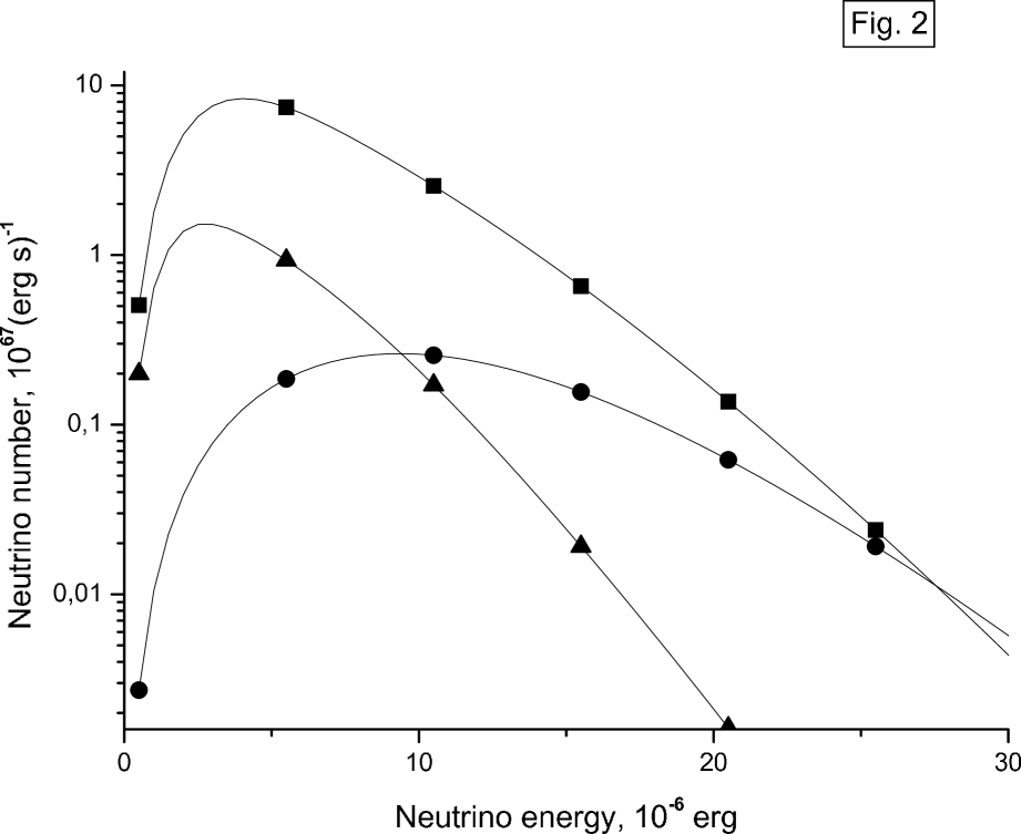
Figure 2: Spectra of the neutrinos at times $t^{*}=-10.55$ s (curve with squares, luminosity $10\%$ of the maximum), $t^{*}=-1.25$ s (curve with circles, maximum luminosity), and $t^{*}=7.25$ s (curve with triangles, luminosity $10\%$ of the maximum).

Figure 2 presents neutrino spectra at times $t^{*}=-1.25$ s (curve with circles), $t^{*}=-10.55$ s (curve with squares), and $t^{*}=7.25$ s (curve with triangles), with the luminosity being maximum in the first case and $10\%$ of the maximum in the latter two cases. We can see that the spectrum becomes softer with time due to the influence of the redshift.

6 CONCLUSION

The model presented here can be applied with source functions (12) with fairly arbitrary shapes. Our approximation that the shape of the spectrum of the radiating matter does not depend on temperature in our derivation of formula (70) was made only to simplify the calculation. If the source function cannot be presented in the form (72), it must be expanded in a Loran series,

$$f(q,a)=\sum_{n=-\infty}^{\infty}y_{n}(q)a^{n}$$

and the linearity of the problem taken into account; i.e., it is necessary to obtain a solution for each term of the series separately and then sum the results.

Thus, our solution for the properties of a neutrino pulse arising during the collapse of a supermassive star can be used to consider various processes that generate neutrinos (plasma neutrinos, pair annihilation, and so forth). There is no question that the solution does not model a real collapse completely accurately; in particular, the assumption that the star is uniform during the collapse is crude. However, the resulting solution is very simple while also displaying all the properties that are characteristic of real systems. This makes it possible to obtain light curves and spectra for such stars that are close to the real curves without having to carry out complex three-dimensional computations.

7 ACKNOWLEDGMENTS

One of the authors (A. N. B.) thanks S. L. Karepov and Yu.I. Khanukaev for useful discussions. This work was partially supported by the Russian Foundation for Basic Research (project codes 01-02-06146, 02-02-06596, 02-02-16900) and INTAS (INTAS-EKA grant 99-120 and INTAS grant 00-491).

References

- [1] Ya. B. Zeldovich, (1963), At. Energ. 521, 49.
- [2] M.A. Podurets, (1964), Astron.Zh., 41, 28 [Sov.Astron., (1964), 8, 19].
- [3] Ames, W.L., Thorn, K.S., (1968), Ap.J., 151, 659.
- [4] Shapiro, S.L., (1996), Phys. Rev. D., 40, 1858.
- [5] Shapiro, S.L., (1996), Ap.J., 472, 308.
- [6] Shi, X., Fuller, G.M., (1998), Ap.J., 503, 307.
- [7] Linke, F., Font, J.A., Janka, H.T., et al., (2001), Astron.Ap., 376, 568.
- [8] Landau, L.D., Lifshitz, E.M. // The Classical Theory of Fields, any edition.
- [9] Lindquist, R.W., (1966), Annals of Physics, 37, 487.
- [10] Ya.B. Zeldovich & I.D. Novikov, Relativistic Astrophysics (Nauka, Moscow, 1967) [in Russian].
- [11] G. S. Bisnovatyi-Kogan, (1968), Astron.Zh. 45, 74 [Sov.Astron., (1968), 12, 74].
- [12] Schinder, P.J., Schramm, D.N., Wiita, P.J., et.al., (1987), Ap.J., 313, 531.
- [13] Itoh, N., Adachi, T., Nakagawa, M., et.al., (1989), Ap.J., 339, 354.