Formation and Size-Dependence of Vortex Shells in Mesoscopic Superconducting Niobium Disks

Abstract

Recent experiments [I.V. Grigorieva et al., Phys. Rev. Lett. 96, 077005 (2006)] on visualization of vortices using the Bitter decoration technique revealed vortex shells in mesoscopic superconducting Nb disks containing up to $L=40$ vortices. Some of the found configurations did not agree with those predicted theoretically. We show here that this discrepancy can be traced back to the larger disks with radii $R\sim 1$ to 2.5$\mu$m, i.e., $R\sim 50-100\xi(0)$ used in the experiment, while in previous theoretical studies vortex states with vorticity $L\leq 40$ were analyzed for smaller disks with $R\sim 5-20\xi(0)$. The present analysis is done for thin disks (mesoscopic regime) and for thick (macroscopic) disks where the London screening is taken into account. We found that the radius of the superconducting disk has a pronounced influence on the vortex configuration in contrast to, e.g., the case of parabolic confined charged particles. The missing vortex configurations and the region of their stability are found, which are in agreement with those observed in the experiment.

I Introduction

A mesoscopic superconducting disk is the most simple system to study confined vortex matter where effects of the sample boundary plays a crucial role. At the same time, it is a unique system because just by using disks of different radii, or by changing the external parameters, i.e., the applied magnetic field or temperature, one can cover — within the same geometry — a wide range of very different regimes of vortex matter in mesoscopic superconductors.

Early studies of vortex matter in mesoscopic disks were focused on a limiting case of thin disks or disks with small radii in which vortices arrange themselves in rings GPN97 ; DSPGL97 ; lozovik ; SPB98 ; SPL99 ; BPS01 , in contrast to infinitely extended superconductors where the triangular Abrikosov vortex lattice is energetically favorable tinkham ; degennes ; abrikosov . Several studies were devoted to the questions: i) how the vortices are distributed in disks, ii) which vortex configuration is energetically most favorable, and iii) how the transition between different vortex states occurs. Lozovik and Rakoch lozovik analyzed the formation and melting of two-dimesional microclusters of particles with logarithmic repulsive interaction, confined by a parabolic potential. The model was applied, in particular, to describe the behaviour of vortices in small thin (i.e., with a thickness smaller than the coherence length $\xi$) grains of type II superconductor. Buzdin and Brison buzdin studied vortex structures in superconducting disks using the image method, where vortices are considered as point-like “particles”, i.e., within the London approximation. Palacios palacios calculated the vortex configurations in superconducting mesoscopic disks with radius equal to $R=8.0\xi$, where two vortex shells can become stable. The demagnetization effects were included approximately by introducing an effective magnetic field. Geim et al. geim studied experimentally and theoretically the magnetization of different vortex configurations in superconducting disks. They found clear signatures of first- and second-order transitions between states of the same vorticity. Schweigert and Peeters SPL99 analyzed the transitions between different vortex states of thin mesoscopic superconducting disks and rings using the nonlinear Ginzburg-Landau (GL) functional. They showed that such transitions correspond to saddle points in the free energy: in small disks and rings — a saddle point between two giant vortex (GV) states, and in larger systems — a saddle point between a multivortex state (MV) and a GV and between two MVs. The shape and the height of the nucleation barrier was investigated for different disk and ring configurations. Milošević, Yampolskii, and Peeters MYPB02 studied vortex distributions in mesoscopic superconducting disks in an inhomogeneous applied magnetic field, created by a magnetic dot placed on top of the disk. It was shown MPB03 , that such an inhomogeneous field can lead to the appearance of Wigner molecules of vortices and antivortices in the disk.

In the work of Baelus et al. BCPB04 the distribution of vortices over different vortex shells in mesoscopic superconducting disks was investigated in the framework of the nonlinear GL theory and the London theory. They found vortex shells and combination of GV and vortex shells for different vorticities $L$.

Very recently, the first direct observation of rings of vortices in mesoscopic Nb disks was done by Grigorieva et al. grigorieva using the Bitter decoration technique. The formation of concentric shells of vortices was studied for a broad range of vorticities $L$. From images obtained for disks of different sizes in a range of magnetic fields, the authors of Ref. grigorieva traced the evolution of vortex states and identified stable and metastable configurations of interacting vortices. Furthermore, the analysis of shell filling with increasing $L$ allowed them to identify magic number configurations corresponding to the appearance of consecutive new shells. Thus, it was found that for vorticities up to $L=5$ all the vortices are arranged in a single shell. Second shell appears at $L=6$ in the form of one vortex in the center and five in the second shell [state (1,5)], and the configurations with one vortex in the center remain stable until $L=8$ is reached, i.e., (1,7). The inner shell starts to grow at $L=9$, with the next two states having 2 vortices in the center, (2,7) and (2,8), and so on. From the results of the experiment grigorieva it is clear that, despite the presence of pinning, vortices generally form circular configurations as expected for a disk geometry, i.e., the effect of the confinement dominates over the pinning. Similar shell structures were found earlier in different systems as vortices in superfluid He campbell ; hess ; stauffer ; totsuji ; tsuruta , charged particles confined by a parabolic potential BePB94 , dusty plasma plasma , and colloidal particles confined to a disk colloids . Note that the behavior of these systems is similar to that of vortices in thin mesoscopic disks, thus our approach of Sec. II can be used for better understanding of the behavior of various systems of particles confined by a parabolic potential and charachterized by a logarithmic interparticle interaction (e.g., vortices in a rotating vessel with superfluid He campbell ; hess ; stauffer ; totsuji ; tsuruta ). In contrast, our results presented in Sec. III are specific for vortices in thick large mesoscopic superconducting disks, where the London screening is important, and the intervortex interaction force is described by the modified Bessel function.

The filling of vortex shells was experimentally analyzed grigorieva for vorticities up to $L=40$. Many configurations found experimentally agree with earlier numerical simulations for small $L$ which were done for mesoscopic disks with radii as small as $R\approx 6-8\xi(0)$, although the disks used in the experiments grigorieva were much larger, $R\approx 50-100\xi(0)$. At the same time, some theoretically predicted configurations were not found in the experiment, such as states (1,8) for $L=9$ and (1,9) for $L=10$. The difference between vortex states in small and large disks becomes even more striking for larger vorticities $L$. In small disks with radii of a few $\xi$, the formation of GVs is possible if the vorticity $L$ is large enough, e.g., in disks with $R=6\xi$, a GV with $L=2$ appears in the center for total vorticity $L=14$, but for vorticities $L>14$, all the vortices form a GV BCPB04 . Obviously, this boundary-induced formation of GVs is possible only in the case of small disks: in large disks vortices instead form the usual Abrikosov lattice which is distorted near boundaries.

The aim of the present paper is to theoretically analyze vortex states, using Molecular-Dynamics (MD) simulations, in rather large mesoscopic superconducting disks and thus to study the crossover between mesoscopic and macroscopic disks, i.e., the regime corresponding to the Nb disks used in the recent experiments of Ref. grigorieva and to look for the missing vortex configurations in the earlier simulations. We analyzed the region of stability of those configurations and performed a systematic study of all possible vortex configurations. We found that the radius of the disk has an influence on the vortex shell structure, in contrast to the case of charged particles confined by a parabolic potential BePB94 . This analysis was done for thin mesoscopic disks and for thick disks where the London screening becomes pronounced. We also perform calculations of vortex configurations using the GL equations, and we compare these results to the ones obtained within the MD simulations. The calculated vortex configurations agree with those observed in the experiment grigorieva .

The paper is organized as follows. In Sec. II, we discuss thin mesoscopic disks. The model and the simulation method is described in Sec. II.A. In Sec. II.B, we discuss different vortex configurations and the formation of vortex shells. We analyze the ground states and metastable states for different vorticities in Sec. II.C, using a statistical study, similar to the one employed in the experiments of Ref. grigorieva , by starting with many random vortex configurations and comparing the energies of different vortex configurations. Based on that analysis we reconstructed the “radius $R-$magnetic field $H$” phase boundary (Sec. II.D). In Sec. III, we study the crossover from thin mesoscopic to thick macroscopic disks, and we analyze the impact of the London screening on the vortex patterns. In Sec. IV, we calculate the crucial vortex configurations in disks using the GL equations, and we compare them to the results obtained within the MD simulations. A summary of the results obtained in this work is given in Sec. V.

II Mesoscopic disks

II.1 Theory and simulation

In this Section, we consider a thin disk with thickness $d$ and radius $R$ such that $\lambda_{eff}\gg R\gg\xi\gg d$, placed in a perpendicular external magnetic field $\bm{H}_{0}$. Here $\lambda_{eff}=\lambda^{2}/d$ is the effective London penetration depth for a thin film, $\lambda$ is the bulk London penetration depth, and $\xi$ is the coherence length. We follow here the theoretical approach developed in CBPB04 ; BCPB04 ; buzdin for thin disks and we use the original dimensionless variables used in those works. Thus, following CBPB04 ; BCPB04 the lengths are measured in units of the coherence length $\xi$, the magnetic field in units of $H_{c2}=c\hbar/2e\xi^{2}=\kappa\sqrt{2}H_{c}$, and the energy density in units of $H_{c}^{2}/8\pi$. The number of vortices, or vorticity, will be denoted by $L$. In a thin disk in which demagnetization effects can be neglected the free energy in the London limit can be expressed as CBPB04 ; BCPB04 ; buzdin

$$G_{L}=\sum_{i=1}^{L}\left({\epsilon}_{i}^{s}+\sum_{j=1}^{i-1}{\epsilon}_{ij}\right)+{\epsilon}^{core}+{\epsilon}^{field},$$ (1)

where the potential energy of vortex confinement consists of two terms:

$${\epsilon}_{i}^{s}={\epsilon}_{i}^{self}+{\epsilon}_{i}^{shield}$$ (2)

i.e., the interaction energy between the $i$th vortex and the radial boundary of the superconductor,

$${\epsilon}_{i}^{self}=\left(\frac{2}{R}\right)^{2}ln(1-r_{i}^{2}),$$ (3)

and the interaction energy between the $i$th vortex and the shielding currents,

$${\epsilon}_{i}^{shield}=-2H_{0}(1-r_{i}^{2}).$$ (4)

In Eq. (1),

$${\epsilon}_{ij}=\left(\frac{2}{R}\right)^{2}ln\left[\frac{(r_{i}r_{j})^{2}-2{\rm\bf r}_{i}\cdot{\rm\bf r}_{j}+1}{r_{i}^{2}-2{\rm\bf r}_{i}\cdot{\rm\bf r}_{j}+r_{j}^{2}}\right]$$ (5)

is the repulsive interaction energy between vortices $i$ and $j$. Here ${\rm\bf r}_{i}={\rho}_{i}/R$ is the distance to the vortex normalized to the disk radius. The divergence arising when $i=j$ is removed in Eq. (5) using a cutoff procedure (see, e.g., abrikosov ; book ; buzdin ) which assumes the replacement of $\mid{\rho}_{i}-{\rho}_{j}\mid$ by $a$ (or by $a\xi$ in not normalized units) for $i=j$. Finally, $\epsilon^{core}=(2/R)^{2}L$ $ln(R/a)$ and $\epsilon^{field}=R^{2}H_{0}^{2}/4$ are the energies associated with the vortex cores and the external magnetic field, respectively. Notice that the energy of the vortex cores $\epsilon^{core}$ becomes finite due to the cutoff procedure and is strongly dependent on the cutoff value $a\xi$ BCPB04 . Here we use for the vortex size $a=\sqrt{2}\xi$; this choice, as shown in Ref. CBPB04 , makes the London and the Ginzburg-Landau free energies to agree with each other.

From the expression of the free energy given by Eqs. (1-5), we obtain the force acting on each vortex, $-\nabla_{k}G(\bm{\rho}_{i},\bm{\rho}_{j}),$ where $-\nabla_{k}$ is the gradient with respect to the coordinate $\bm{\rho}_{k}$. This yields a force per unit length,

$${\rm\bf F}_{i}={\rm\bf F}_{i}^{s}+\sum_{k\neq i}{\rm\bf F}_{i,k}^{int},$$ (6)

in units of $H_{c}^{2}\xi/8\pi$, where the summation over $k$ runs from 1 to $L$, except for $k=i$. The first term describes the vortex interaction with the current induced by the external field and with the interface,

$${\rm\bf F}_{i}^{s}=\left(\frac{2}{R}\right)^{3}\left(\frac{1}{1-r_{i}^{2}}-\frac{H_{0}R^{2}}{2}\right){\rm\bf r}_{i}.$$ (7)

The second term is the vortex-vortex interaction

$${\rm\bf F}_{i,k}^{int}=\left(\frac{2}{R}\right)^{3}\left(\frac{{\rm\bf r}_{i}-{\rm\bf r}_{k}}{\mid{\rm\bf r}_{i}-{\rm\bf r}_{k}|^{2}}-r_{k}^{2}\frac{r_{k}^{2}{\rm\bf r}_{i}-{\rm\bf r}_{k}}{\mid r_{k}^{2}{\rm\bf r}_{i}-{\rm\bf r}_{k}|^{2}}\right).$$ (8)

The above equations allow us to treat the vortices as point-like particles and the forces resemble those of a two-dimensional system of charged particles with $1/r$ repulsive interaction confined by some (usually, parabolic) potential BePB94 . However, the inter-vortex interaction in our system is different from $1/r$, and the confined potential differs from parabolic and depends on the applied magnetic field.

To investigate different vortex configurations, we perform MD simulations of interacting vortices in a disk (see, e.g., Ref. CBPB04 ), starting from randomly distributed vortex positions. The final configurations were found after typically $10^{6}$ MD steps.

In order to find the ground state (or a state with the energy very close to it) we perform many (typically, one hundred) runs of simulations for the same number $L$ of vortices starting each time from a different random initial distribution of vortices. As a result, we obtain a set of final configurations which we analyze statistically, i.e., we count probabilities to find the different configurations with the same vorticity $L$, e.g., configurations (1,8) and (2,7) for $L=9$. We can expect that the configuration which appears with the highest probability is the ground state of the system, i.e., the vortex state with the lowest energy. (However, in some cases, i.e., for particular vortex configurations the highest probability state turns out to be not always the ground state configuration. One of these special cases will be addressed below.) This approach corresponds to the analysis done in the experiment grigorieva .

The MD simulation was performed by using the Bardeen-Stephen equation of motion

$$\eta\frac{d\rho_{i}}{dt}={\rm\bf F}_{i},$$ (9)

where $i$ denotes the $i$th vortex, $\eta$ is the viscosity coefficient $\eta\sim\Phi_{0}H_{c2}/\rho_{n}c^{2}$, with $\rho_{n}$ being the normal-state resistivity; $\Phi_{0}=hc/2e$ is the magnetic flux quantum. The time integration was accomplished by using the Euler method.

II.2 Vortex configurations for different $L$: Formation of vortex shells

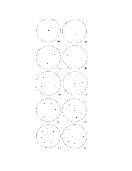
Figure 1: The evolution of vortex configurations for the states with vorticity increasing from $L=1$ to 10, in mesoscopic superconducting disks with radius $R=50\xi$. Vortices form one-shell configurations for $L=1$ to 5 (a)-(e). The formation of second shell starts for $L=6$ (f). The inner shell contains 1 vortex at the center for $L=5$ to 8, while new vortices fill the outer shell (f-h). For $L=9$, second vortex appears in the inner shell (i), and then second shell again starts to grow for $L=10$ (j).

To study the formation of vortex shells in mesoscopic supeconducting disks, here we analyze the evolution of vortex configurations with increasing number of vortices, $L$, in a disk with radius $R=50\xi$. The results of our calculations for $L=1$ to 10 are presented in Fig. 1. When the vorticity $L$ of the sample increases, the vortex configurations evolve with increasing applied magnetic field as follows: starting from a Meissner state without vortex, then one appears in the center (Fig. 1(a)), which we denote as (1), then two symmetrically distributed vortices, (2) (Fig. 1(b)). Further increasing the magnetic field results in the formation of triangular, (3) (Fig. 1(c)) and square like (4)(Fig. 1(d)) vortex patterns in the sample, and in a five-fold symmetric pattern, (5), shown in Fig. 1(e). When the vorticity $L$ increases from 5 to 6, a vortex appears in the center of the disk, thus starting to form a second shell of vortices in the disk (Fig. 1(f)). We denote the corresponding two-shell vortex state containing 1 vortex in the first shell and 5 vortices in the second shell as (1,5). Two-shell configurations with one vortex in the center and newly generated vortices added to the outer shell remain for the states (1,6) with $L=7$ (Fig. 1(g)), and (1,7) with $L=8$ (Fig. 1(d)). The number of vortices in the inner shell begins to grow at $L=9$ thus forming subsequently configurations (2,7)(Fig. 1(i)), and (2,8) with $L=10$ (Fig. 1(j)).

Note that in earlier theoretical works on vortices in mesoscopic superconducting disks, a configuration (1,8) for $L=9$ was predicted BCPB04 ; lozovik as a ground state in smaller disks, which however was not observed in the experiment grigorieva as a stable state (the special case $L=9$ will be discussed in Sec. III for the model of a thick disk, i.e., $d\gg\lambda$, relevant to the experiment grigorieva , where the London screening in large disks, i.e., $R>\lambda$, is taken into account). Our calculations show that the multivortex states with two vortices in the center and the other vortices on the outer shell can exist till $L=14$. For $L>14$, the inner shell starts growing again till $L=16$, which means that a newly nucleated vortex will be generated in the inner shell, while the number of vortices in the outer shell stays the same. We found that those configurations are (3,11) for $L=14$, (4,11) for $L=15$, and (5,11) for $L=16$. At $L=17$, a vortex appears in the center, thus giving rise to the formation of a third shell with one vortex in the center. With increasing number of vortices in the disk, the next three vortices are added to the outermost shell, after which all three shells grow intermittently till $L=32$. The fourth shell appears at $L=33$ in the form of one vortex in the center. The borderline vortex configurations illustrating the formation of new shells are presented in Fig. 2. We summarize the vortex configurations found for vorticities $L=1$ to 33 in Table 1.

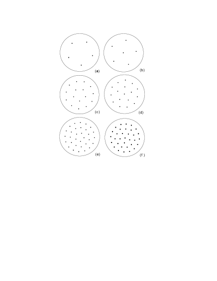
Figure 2: The borderline vortex configurations for: one shell, starting from state (1) for $L=1$ to state (5) for $L=5$ (a), two shells, states (1,5) for $L=6$ (b) to (5,11) for $L=16$ (c), three shells, states (1,5,11) for $L=17$ (d) to (5,11,16) for $L=32$ (e), four shells, starting from state (1,5,11,16) for $L=33$ (f), for disks with radius $R=50\xi$.

It is appropriate to mention that in our numerical calculations using the vortex-vortex interaction force, Eq. (8), the obtained vortex patterns for some $L$ are different from those found in Ref. lozovik for particles with logarithmic interaction, confined by a parabolic potential, even in case when the interaction with images was taken into account. Although for many vorticities $L$ both approaches result in the same “robust” configurations (i.e., less sensitive to details of interparticle interactions), there is essential difference in configurations for some other vorticities. The lowest vorticity for which our results deviate from those obtained in Ref. lozovik is $L=9$: this special case is described in detail below. Note, for instance, differences in three-shell configurations: (1,5,12) (our approach, see Table 1) [and (1,6,11) lozovik ] for $L=18$, (1,7,12) [(1,6,13)] for $L=20$, (1,8,13) [(1,7,14)] for $L=22$, (2,8,13) [(1,8,14)] for $L=23$, (3,10,15) [(4,9,15)] for $L=28$, (5,10,16) [(4,10,17)] for $L=31$, and (5,11,16) [(4,11,17)] for $L=32$. Moreover, the filling of next (fourth) shell starts, according to our calculations, for $L=33$ (i.e., (1,5,11,16)) while in Ref. lozovik this transition occurs for $L=34$. As noticed in Ref. lozovik , the interaction with images leads to the stabilization of configurations with larger number of vortices on inner shells. While in lozovik this tendency was revealed only in rather large clusters (i.e., the appearance of different configurations for $L=45$: i) (2,8,14,21), without interaction with images, and ii) (3,8,14,20), if the interaction with images is taken into account), we found that the stabilization of vortex shell structures with a larger number of vortices on inner shells occurs for vorticities $L\geq 20$, due to the interaction with images and with the shielding current induced by increasing magnetic field at the boundaries of the disk wecorbino .

Note that, although here we employ the model of a thin mesoscopic disk, the results of our calculations for the filling of vortex shells perfectly match those discovered in the experiment grigorieva (where the disks were rather thick) for vorticities $L=1$ to 40. The vortex configurations calculated in this section using many runs of simulations with random initial distributions, as will be shown below, are not always the ground-state configurations. The obtained results imply that the size of the disk influences the vortex configurations in superconducting disks. This will be clearly demonstrated in Sec. III where we consider thick disks and we show that the London screening has a pronounced impact on the vortex configurations in disks of different radii.

$L$	1	2	3	4	5	6	7	8	9	10	11
Config.	1	2	3	4	5	(1,5)	(1,6)	(1,7)	(2,7)	(2,8)	(3,8)
$L$	12	13	14	15	16	17	18	19	20	21	22
Config.	(3,9)	(4,9)	(4,10)	(4,11)	(5,11)	(1,5,11)	(1,5,12)	(1,6,12)	(1,7,12)	(1,7,13)	(1,8,13)
$L$	23	24	25	26	27	28	29	30	31	32	33
Config.	(2,8,13)	(2,8,14)	(3,8,14)	(3,9,14)	(3,9,15)	(3,10,15)	(4,10,15)	(4,10,16)	(5,10,16)	(5,11,16)	(1,5,11,16)

Table 1: Formation of vortex shells in mesoscopic superconducting disks: vortex configurations for different vorticities $L$.

II.3 The ground state and metastable states

As described in Sec. II.A, in order to find the ground state of the system (or a state with energy very close to it), we performed many (usually one hundred) simulations for the same number of vortices. In most cases, always one configuration dominated over the other possible configurations for a certain vorticity $L$, which was identified as the “ground state”. However, for some vortex configurations competing states appeared with comparable probabilities.

Let us now consider those special cases. For instance, it follows from our calculations that two configurations, (1,8) and (2,7), are possible for the same vorticity $L=9$. They are shown in Figs. 3(c),(d) (another example of competing states with the same vorticity, e.g., $L=17$, are the three-shell configuration (1,5,11) and the two-shell configuration (5,12) which are shown in Figs. 3(a),(b), correspondingly). We found that the configuration (2,7) is the ground state for $L=9$ in a disk with radius $R\leq 11\xi$ (see the $R-H$ phase diagram in Fig. 6) in a certain range of magnetic fields. In very large disks with $R\gtrsim 50\xi$ the vortex state (2,7), although being a metastable state, is the highest probability state. Note that configuration (2,7) was also found as a ground state for the system of charged particles BePB94 . At the same time, as it was shown in Ref. BCPB04 using the GL theory, in small superconducting disks (e.g., for radius $R=6\xi$), this configuration occurred to be a metastable state, while state (1,8) was found as the ground energy state. This clearly shows that the ground state configuration for a certain $L$ depends on the radius of the disk.

II.3.1 Statistical study of different vortex states

In the experiments grigorieva , vortex configurations were monitored in large arrays of similar mesoscopic disks (dots). This allowed them to study the statistics of the appearance of different vortex configurations in practically the same disk. The results show that, e.g., in a disk with radius $R=1.5\mu m$ and magnetic field $H_{0}=60Oe$, configuration (2,8) for $L=10$ appeared more frequently. Other configurations for the same total vorticity $L=10$, e.g., configuration (3,7) appeared only in few cases. Interestingly, not only various configurations with the same total vorticity $L=10$ appeared, but also vortex states with $L=9$ (2,7) and — less frequently — two modifications of the state (1,8): with a ring-like outer shell as well as a square-lattice-like vortex pattern. This statistical study provides indirect information about the ground-state and metastable states.

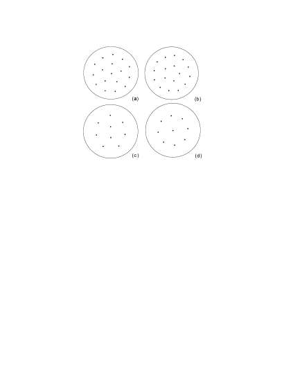
Figure 3: Possible vortex configurations for the total vorticity $L=17$ in a disk with radius $R=50\xi$: (1,5,11) (a) and (5,12) (b); and for the total vorticity $L=9$: (2,7) (c) and (1,8) (d).

We performed a similar investigation of the statistics of the appearance of different vortex states for ideal disks, i.e., in the absence of pinning. One hundred randomly distributed initial states were generated for our statistical study for each set of parameters. We studied the dependence of the appearance of different vortex configurations on the applied magnetic field. For instance, for a disk with radius $R=42\xi$ and the magnetic field varying from $H=0.011H_{c2}$ to 0.015$H_{c2}$, we counted how often the different configurations (e.g., (1,8) and (2,7)) for a total vorticity $L=9$ appeared.

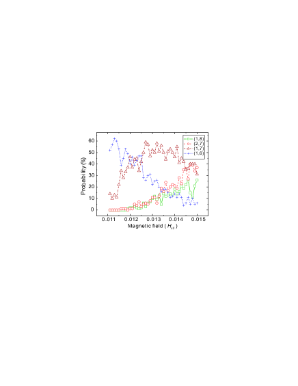
Figure 4: The results of the statistical study of different vortex configurations, i.e., the probability to find a given vortex state as a function of the applied magnetic field, for a disk with radius $R=42\xi$ and varying magnetic field.

The results of such calculations are shown in Fig. 4. At low magnetic field, $H=0.011H_{c2}$, the disk cannot accommodate 9 vortices, so the number of configurations (1,8) and (2,7) is zero, and in most cases we obtain the configurations (1,6) or (1,7) for $L=7$ and $L=8$, respectively. As the magnetic field increases, the probability to find the configurations (1,8) and (2,7) increases, and at the same time the probability to find the configurations (1,6) and (1,7) decreases. Our statistical result shows clearly that in the range of magnetic field shown in Fig. 4 the probability to find configuration (2,7) is always higher than to find configuration (1,8).

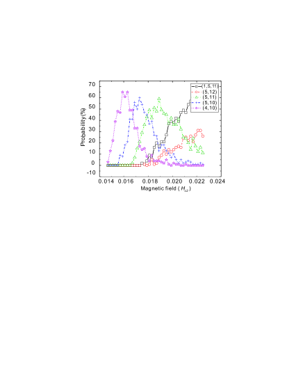
Figure 5: The results of the statistical study of different vortex configurations, for a disk with radius $R=47\xi$ and varying magnetic field.

Similar analysis was performed for a disk with radius $R=47\xi$ where we looked for configurations with total vorticity $L=17$ in the range of the applied magnetic fields from $H=0.014H_{c2}$ to 0.023$H_{c2}$. As shown in Fig. 5, configurations $(4,10)$ for $L=14$, $(5,10)$ for $L=15$, $(5,11)$ for $L=16$, and $(1,5,11)$ and $(5,12)$ for $L=17$ dominate with increasing magnetic field. Note that two configurations, (1,5,11) and (5,12), appeared in the same magnetic field range for $L=17$, and (1,5,11) is always the dominant configuration, i.e., the formation of the third shell starts for vorticity $L=17$ (cp. Ref. grigorieva, ). The results of the statistical study of the configurations (2,7) and (1,8) for small disks ($R=9\xi$) are shown in Fig. 6.

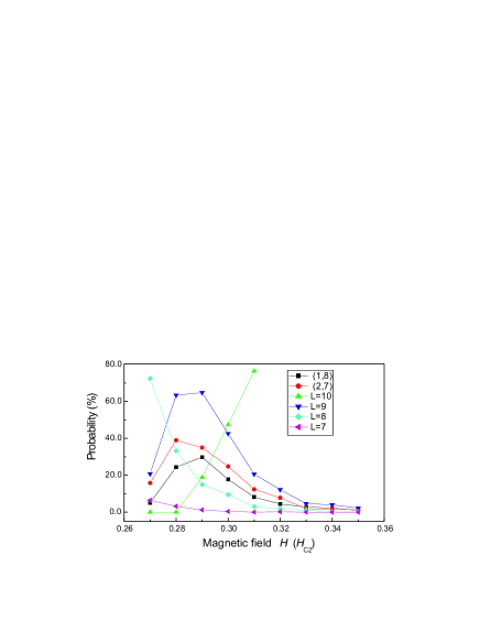
Figure 6: The results of the statistical study of different vortex configurations, for a disk with radius $R=9\xi$ and varying magnetic field. The total probabilities of vortex states with different vorticities $L=7$, 8, 9, and 10, are plotted. For vorticity $L=9$, the probabilities of the two possible configurations (2,7) and (1,8) are also shown.

II.3.2 The $R-H$ phase diagram

To find the region of the existence and stability of vortex states with different vorticity $L$, we performed a direct calculation of their energies using Eq. (1).

As an example, we considered the configurations (1,8) and (2,7) in disks with radius changing in a very wide range from $R=4\xi$ to $R\sim 100\xi$. We change the radius of the disk, and at the same time keep the flux passing through the disk $\Phi=SH_{0}$ the same, in order to keep the same vorticity $L$ in the disk. Here $\Phi$ is the flux passing through the specimen, $H_{0}$ is the applied magnetic field, $S=\pi R_{0}^{2}$ is the surface area of the specimen.

The phase diagram “radius of the disk $R$ – applied magnetic field $H$” is shown in Fig. 7 for $R=7\xi$ to $12\xi$. According to our calculations, for small radii $R<7\xi$, the energy of the configuration (2,7) appears to be always lower than that of configuration (1,8). The total energy for both configurations, (2,7) and (1,8), decreases with increasing magnetic field, and the energy of the state (2,7) is slightly larger than that of the state (1,8).

For disks with radius between $7\xi$ and $12\xi$, the configuration (1,8) has a lower energy than configuration (2,7) for low applied magnetic field. For increasing magnetic field, the reverse is true. The rearrangement of the vortex configurations from the state (1,8) to the state (2,7) is related to the change in the steepness of the potential energy profile (i.e., the vortex-surface interaction, see Eq. (2)) for different points in the $R-H$ phase diagram. The inset of Fig. 7 shows the energy profiles corresponding to points C, D, and E in the phase diagram. Previously, it was shown for charged particles that the particle configiration is influenced by the steepness of the confinement potential kong .

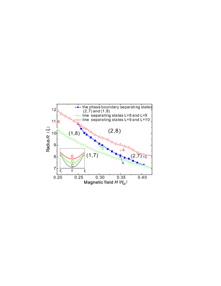
Figure 7: The $R-H$ phase diagram for states with total vorticity $L=9$, for small disks with radii changing in the range: $R=7\xi$ to $R=12\xi$. Points A and B correspond to the configurations (a) and (b) shown in Fig. 10, respectively. The inset shows the confinement potentials (see Eq. (2)) corresponding to the points C, D, and E in the phase diagram.

As it follows from the phase diagram (Fig. 7), we can expect that for larger radii (in the mesoscopic regime, i.e., when $R<\lambda_{eff}$; we show in Sec. III that for thick disks with $R>\lambda_{eff}$ the configuration (2,7) restores as the ground-state configuration). the configuration (1,8) has a lower energy than the state (2,7), in the low magnetic field range. However, the difference in energy between the states (2,7) and (1,8) decreases for increasing $R$, although the energy of the state (1,8) remains lower than that of the state (2,7) for even larger disks (e.g., with radius $R\sim 40-90\xi$ but still “mesoscopic” due to the condition $R<\lambda_{eff}$ valid for very thin disks). This seems to contradict our previous result that the state (2,7) is the highest probability state in large disks (which is also in agreement with the experiment grigorieva ). Thus the question is, whether the highest probability configuration (e.g., state (2,7)) is always the ground state? If not, what is the reason for that?

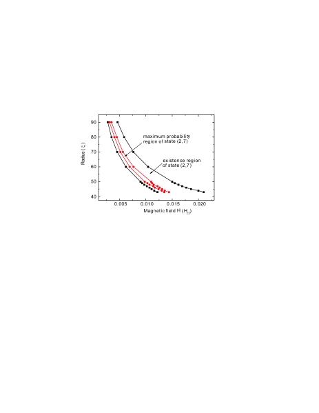
Figure 8: The $R$-$H$ diagram for the vortex state (2,7) calculated using the statistical approach, for large disks with radius $R=40\xi$ to $90\xi$. The area between the red curves and dots shows the region where the state (2,7) has the maximum probability.

To answer this question, we calculated, using the statistical approach described above, the $R-H$ diagram for the state (2,7) (Fig. 8), i.e., the region of the existence of the state (2,7) and the region where the state (2,7) has the highest probability, for radii $R=40\xi$ to $90\xi$. The region of the existence of the state (2,7) as the highest probability state is very narrow although it is well-defined even for very large radii (e.g., $R=90\xi$, see Fig. 8). However, for radii $R\lesssim 40\xi$ this region becomes narrower and unstable, i.e., it can even disappear, giving rise to higher probability of appearance of the state (1,8).

This calculation clearly shows that the highest probability state (2,7) is not the ground state in large disks. The reason of such behavior is that the energy minimum in configurational space corresponding to the state (2,7) is very wide while the competing state (1,8) possesses, although slightly deeper, a much narrower minimum. Thus, statistically the system ends up more often into the wide minimum corresponding to the state (2,7). This is confirmed by a calculation of the potential energy profile which is shown in Fig. 9 as a function of the displacement (i.e., for different vortex configurations, between the initial nonequilibrium configuration (2,7) – through the equilibrium state (2,7) – and the final state (1,8)) of one of the central vortices of the configuration (2,7) during the continuous transition to the configuration (1,8). The position of the other vortices is determined by minimizing the energy. The corresponding changes of the vortex configuration are shown in the inset of Fig. 9. We started from an out-of-equilibrium (2,7) configuration, passed through the equilibrium (2,7) configuration (wide minimum), then passed over the energy maximum, and, finally, ended up at the equilibrium (1,8) configuration (a tail of the transition is also shown for out-of-equilibrium (1,8) configuration) which has slightly lower energy.

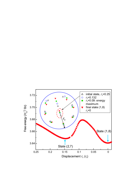
Figure 9: The energy of the system of $L=9$ vortices as a function of the displacement $r_{d}$ (measured in units of the disk radius $r_{0}$ and counted from the center of the disk) of one of the central vortices of the initial configuration (2,7) during the continuous transition to the configuration (1,8). The inset shows the corresponding evolution of the vortex configuration (different symbols show vortex configurations for different dispalcements $r_{d}$ of the vortex marked by red dashed line) during the transition from the state (2,7) to the state (1,8).

III Macroscopic regime: Thick disks

In Sec. II we analyzed in detail the formation of vortex shells in mesoscopic disks. Although we considered rather large disks with radii up to $R\sim 100\xi$, the results obtained in the previous section refer essentially to thin disks: only if the disk’s thickness $d$ is small enough, the $R<\lambda_{eff}=\lambda^{2}/d$ condition is satisfied, i.e., for disks with $R\sim 1\mu$m, $d$ has to be of the order of a few nanometers. Nb disks used in the experiment grigorieva had radius $R=1-2\mu$m and thickness $d=150$nm. For such thick disks with $R>\lambda$ (e.g., $\lambda(0)=90$nm for Nb disks in the experiment grigorieva ), the effects due to London screening become important. In this section, we consider the limit of thick disks with $d\gg\lambda$ and we study how the London screening in the vortex-vortex and vortex-boundary interactions influences the vortex patterns in the disk.

Here we model a cylinder with radius $R$ infinitely long in the $z$-direction by a two-dimensional (2D) (in the $xy$-plane) disk, assuming the vortex lines are parallel to the cylinder axis. This approach was used for studying, e.g., vortex dynamics in periodic md01 ; md0157 ; md02 and quasiperiodic arrays of pinning sites (APS) penrose . As distinct from infinite APSs where periodic boundary conditions are imposed at the boundaries of a simulation cell, here we impose boundary conditions at the edge of the (finite-size) disk, namely, the potential barrier for vortex entry/exit. To study the configurations of vortices interacting with each other and with the potential barrier, we perform simulated annealing simulations by numerically integrating the overdamped equations of motion (unlike in Refs. md01 ; md0157 ; md02 ; penrose , there is no external driving force in our system, and we study the relaxation of initially randomly distributed vortices to the ground-state vortex configuration):

$$\eta{\rm\bf v}_{i}\ =\ {\rm\bf f}_{i}\ =\ {\rm\bf f}_{i}^{vv}+{\rm\bf f}_{i}^{vb}+{\rm\bf f}_{i}^{T}.$$ (10)

Here, ${\rm\bf f}_{i}$ is the total force per unit length acting on vortex $i$, ${\rm\bf f}_{i}^{vv}$ and ${\rm\bf f}_{i}^{vb}$ are the forces due to vortex-vortex and vortex-barrier interactions, respectively, and ${\rm\bf f}_{i}^{T}$ is the thermal stochastic force; $\eta$ is the viscosity, which is set here to unity. The force due to the interaction of the $i$-th vortex with other vortices is

$${\rm\bf f}_{i}^{vv}\ =\ \sum\limits_{j}^{N_{v}}\ f_{0}\ K_{1}\!\left(\frac{\mid{\rm\bf r}_{i}-{\rm\bf r}_{j}\mid}{\lambda}\right)\hat{\rm\bf r}_{ij}\;,$$ (11)

where $N_{v}$ is the number of vortices, $K_{1}$ is the modified Bessel function, $\hat{\rm\bf r}_{ij}=({\rm\bf r}_{i}-{\rm\bf r}_{j})/\mid{\rm\bf r}_{i}-{\rm\bf r}_{j}\mid,$ and

$$f_{0}=\frac{\Phi_{0}^{2}}{8\pi^{2}\lambda^{3}}\;.$$

It is convenient, following the notation used in Refs. md01 ; md0157 ; md02 ; penrose , to express now all the lengths in units of $\lambda$ and all the fields in units of $\Phi_{0}/\lambda^{2}$. The Bessel function $K_{1}(r)$ decays exponentially for $r$ larger than $\lambda$, therefore it is safe to cut off the (negligible) force for distances larger than $5\lambda$. In our calculations, the logarithmic divergence of the vortex-vortex interaction forces for $r\to 0$ is eliminated by using a cutoff for distances less than $0.1\lambda$.

Vortex interaction with the edge is modelled by implying the usual Bean-Levingston barrier bean-levingston ; tinkham ; book . We assume that the repulsive force exerted by the surface current on the vortex at a distance $r$ from the disk edge decays as

$${\rm\bf f}_{i}^{vbc}=\frac{\Phi_{0}H_{0}}{4\pi\lambda}{\rm exp}\left(-\frac{r}{\lambda}\right),$$ (12)

as it does in the case of a semi-infinite superconductor bean-levingston ; tinkham ; book (which is justified for disks with $R\gg\lambda$), and the attractive force due to the vortex interaction with its image is expressed by

$${\rm\bf f}_{i}^{vbi}=-{\rm\bf f}_{i}^{vv},$$ (13)

and

$${\rm\bf f}_{i}^{vb}={\rm\bf f}_{i}^{vbc}+{\rm\bf f}_{i}^{vbi}.$$ (14)

Here we assume that for large enough disks, the distance from the edge to the image is equal to the distance to the vortex.

The temperature contribution to Eq. (10) is represented by a stochastic term obeying the following conditions:

$$\langle f_{i}^{T}(t)\rangle=0,$$ (15)

and

$$\langle f_{i}^{T}(t)f_{j}^{T}(t^{\prime})\rangle=2\,\eta\,k_{B}\,T\,\delta_{ij}\,\delta(t-t^{\prime}).$$ (16)

The ground state of a system of vortices is obtained as follows. First, we set a high value for the temperature, to let vortices move randomly. Then, the temperature is gradually decreased down to $T=0$. When cooling down, vortices interacting with each other and with the edges adjust themselves to minimize the energy, simulating the field-cooled experiments (see, e.g., tonomura-vvm ; togawa ).

Our calculations show that most of the vortex configurations found in Sec. II and in the previous theoretical works on mesoscopic disks CBPB04 remain unchanged also in large disks where the interactions are screened at the London penetration depth $\lambda$. These are stable shell patterns (e.g., (1,6) for $L=7$ and (1,7) for $L=8$, etc.) which were found to be the ground-state configurations of vortices in superconductors CBPB04 , in liquid He campbell , and in a system of charged particles confined by a parabolic potential BePB94 . These stable configurations are mainly determined by the circular shape of the disk, and they are to a much less extend sensitive to the specific interaction potentials between the particles and the boundaries. On the other hand, the “borderline” configurations (i.e., those for which one or more shells start to be filled), e.g., the states (1,8) vs. (2,7) for $L=9$ or the states (2,9) vs. (3,8) for $L=11$, are much more sensitive to the interactions in the disk. For example, for $L=11$ the theory predicts the configuration (3,8) to be the ground state for vortices in He campbell and for charged particles BePB94 , and it is was also observed in the experiment grigorieva in large disks, while the theory predicted CBPB04 the configuration (2,9) in small mesoscopic disks. For $L=9$ the theory predicts that the configuration (1,8) is the ground state for vortices in He campbell and in small mesoscopic superconducting disks CBPB04 , while for charged particles the configuration (2,7) was predicted BePB94 . This vortex configuration, (2,7), was also observed in the experiment grigorieva with Nb disks. In Sec. II we showed that in mesoscopic disks the state (2,7) had the highest probability to appear (due to the wide potential energy minimum related to this state), although it was not the lowest energy configuration, but instead the (1,8) configuration was the ground state.

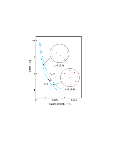
Figure 10: The $R-H$ phase diagram for vortex states with total vorticity $L=9$ in case of a thick disk. The area between the dashed blue curves shows the region where the states with $L=9$ are the ground state. The boundary separating the states (1,8) (small radii) and (2,7) (large radii) are shown by solid red squares. The insets show the corresponding vortex patterns, (1,8) and (2,7).

In case of thick disks as considered here, the calculations show the crossover behavior of the vortex patterns from the state (1,8) to (2,7) with increasing radius of the disk. The phase diagram in Fig. 10 illustrates this behavior. Note that the potential barrier at the disk edge becomes extremely low for low values of the applied magnetic field $H_{0}$ when we have a large radius of the disk. This means that it is very difficult to stabilize a vortex state with only few vortices in such a large disk (in experiment, and also in the numerical calculations using the Ginzburg-Landau equations) because for even very low barrier at the boundary many vortices can enter the sample without any appreciable change of the flux inside the disk. The lines separating the states with different vorticities (shown by dashed lines in Fig. 10) are calculated here assuming the flux inside the disk is on average equal to the applied magnetic field $H_{0}$ multiplied by the area of the disk. The calculated line separating the states (1,8) and (2,7) is shown by solid squares. The phase diagram shows that in relatively small disks with radius $R\lesssim 5\lambda$ (that is $R\lesssim 30\xi$ in case of Nb disks grigorieva ), the configuration (1,8) is the ground state while for larger disks we find the state (2,7), in agreement with the experiment grigorieva .

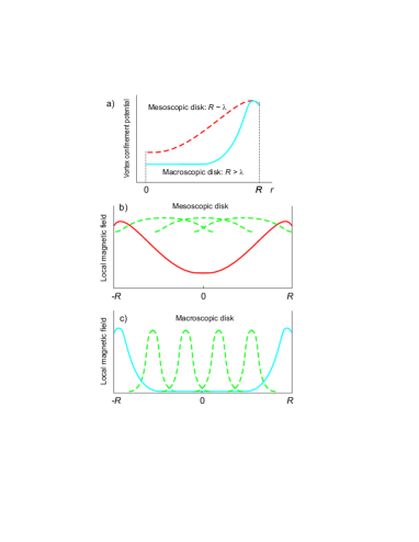
Figure 11: The vortex confinement energy profiles for: mesoscopic disk ($R\sim\lambda$) and for macroscopic disk ($R>\lambda$) (a). Schematic plots illustrating the magnetic field profiles (green dashed curves) of the interacting vortices in: mesoscopic disk (solid red curve shows the vortex confinement potential) (b), and in macroscopic disk (solid blue curve shows the vortex confinement potential) (c).

This crossover behaviour could be understood in the following way. In Fig. 11(a) we plot the vortex confinement potential profiles for a mesoscopic disk ($R\sim\lambda$) and for a macroscopic disk ($R>\lambda$). In a mesoscopic disk, all the vortices interact with the screening current which extends inside the disk. In a macroscopic disk, only the outer-shell vortices feel the screening current. More importantly, the intervortex interaction changes in a disk with the London screening: in a mesoscopic disk, each vortex interacts with all other vortices since the currents created by the vortices strongly overlap (see Fig. 11(b)), and the minimum potential energy is reached when the sum of all the intervortex distances is maximum, i.e., for the configuration (1,8). In a macroscopic disk, the intervortex interaction is very weak, and each vortex interacts only with its closest neighbor through the tails of the currents associated with each vortex (see Fig. 11(c)), and the minimum potential energy is reached when the sum of closest-neighbor intervortex distances is maximum, i.e., for the configuration (2,7). The vortex pattern (2,7) in a large disk (see inset in Fig. 10) resembles a distorted Abrikosov vortex lattice in an infinite superconductor which is stabilized by intervortex interactions in the absence of boundaries (note that the outer-shell vortices are relatively closer to the boudary and the two vortices in the inner shell are slightly out of the center minimizing the interaction energy with the 2 and 3 neighbors).

The calculated crossover behavior found here is consistent with the $R-H$ phase diagram obtained in Sec. II for mesoscopic disks (Fig. 7) that predicted the configuration of (1,8) as the ground state for radii $R\gtrsim 10\xi$. Thus, according to the phase diagrams for mesoscopic disks (Fig. 7) and for macroscopic disks (Fig. 10), there are two crossovers between the states (1,8) and (2,7): the configuration (1,8) is the ground state in disks with radius $10\xi\lesssim R\lesssim 30\xi$, while the configuration (2,7) occurs to be the ground state in large disks with $R\gtrsim 5\lambda$ (i.e., $R\gtrsim 30\xi$ in Nb disks grigorieva ) and in very small disks with $R\lesssim 10\xi$. The mechanism of the second crossover for very small disks is very different from that for large disks, and the transition (1,8)$\to$(2,7) happens in very small disks due to a strong overlap of the vortex cores in the outer eight-vortex shell: the vortices cannot accomodate on the outer shell and one of them is pushed towards the interior of the disk (note that for even smaller disks the configuration (2,7) collapses to a giant-vortex state). This behavior will be demonstrated in Sec. IV using the Ginzburg-Landau theory.

IV Comparison with the GL theory

In order to go beyond the London approximation we used also the Ginzburg-Landau (GL) equations to calculate the free energy and find the ground state. Within the GL approach vortices are no longer point-like “particles” but extended objects. The expression for the dimensionless Gibbs free energy is (see, e.g., Ref. SPB98 ):

$$G=V^{-1}\int_{V}[2({\rm\bf A}-{\rm\bf A}_{0})\cdot{\rm\bf j}_{2D}-\mid\Psi\mid^{4}]d{\rm\bf r},$$ (17)

with $\psi({\rm\bf r})$ the order parameter, ${\rm\bf A}({\rm\bf A}_{0})$ the vector potential of the total (applied) magnetic field and ${\rm\bf j}_{2D}$ the superconducting current. By comparing the dimensionless Gibbs free energies of the different vortex configurations, we find the ground state. Similarly we could find the two stable configurations (2,7) and (1,8) in a disk with vorticity $L=9$ as we found within the MD simulations in Secs II and III.

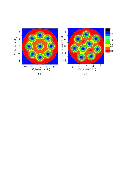
Figure 12: Contour plots of the Cooper-pair density of state (2,7) for $R=8.3\xi$ (a), and state (1,8) for $R=8.2\xi$ (b), in an applied magnetic field $H_{0}=0.35H_{c2}$. Blue and red regions correspond to low and high Cooper-pair density, respectively.

The results of our calculations of the order parameter distribution using the GL equations (for simplicity, this was done for zero disk thickness, $d\to 0$, i.e., in the limit of extreme type II superconductor, for a given applied magnetic field, i.e., only first GL equation was solved) for the total vorticity $L=9$ are shown in Fig. 12. The states (2,7) and (1,8) are shown in the phase diagram (see Fig. 7) by symbols A and B, respectively. Samples with different radius were examined for a fixed external magnetic field $H=0.35H_{c2}$. For a disk with radius $R=8.2\xi$, our calculation gives (1,8) as the ground vortex state. When the radius of the disk is increased, the energy of (1,8) is the lowest one till $R=8.25\xi$, after which configuration (2,7) becomes the ground state. This compares with our results of Sec. II using the London theory where we found that the transition (1,8) $\rightarrow$ (2,7) occurred for $R=8.13\xi$ when $H=0.35H_{c2}$. Thus, the results of a calculation of the vortex configurations within the GL, with an appropriate choice of the radius and external parameters, confirms the crossover behavior found in Sec. II.

V Conclusions

In this work, we studied the vortex configurations in mesoscopic superconducting thin disks and in thick disks taking into account the London screening, using the Molecular-Dynamics simulations of the Langevin-type equations of motion and confirmed these results, in case of small disks, using the more extended Ginzburg-Landau functional theory.

This study was motivated by recent experiments by Grigorieva et al. grigorieva who observed vortex shell structures in mesoscopic Nb disks with $R\sim 1-2.5\mu$m by means of the Bitter decoration technique. It was shown in those experiments, that in disks with vorticity ranging from $L=1$ to 40, vortices fill the disk according to specific rules, forming well-defined shell structures, as earlier predicted in Ref. BePB94 . They analyzed the formation of these shells which resulted in a “periodic table” of formation of shells. It was shown that most of the experimentally observed configurations for small $L$ agreed with those theoretically predicted earlier BCPB04 ; BePB94 . At the same time, some of the configurations which were observed in these experiments were not found earlier in vortex systems (although they were shown to appear in systems of charged particles and in superfluids).

In this work, we found the rules according to which the shells are filled with vortices for increasing applied magnetic field. In particular, it was shown in our calculations, that for the vortex configurations with the number of vortices up to $L=5$, the vortices form a single shell. The formation of a second shell starts from $L=6$. Similarly, the formation of a third shell starts at $L=17$, and of a fourth shell at $L=33$. These theoretical findings are in agreement with the results of the experimental observations of Ref. grigorieva . Moreover, we found those states which were observed in the experiments but not found in previous calculations. Thus, we filled the missing states in the “periodic table” of vortex shells in mesoscopic disks. We studied in detail the region of parameter space where those states exist, and compared the obtained results to previous theoretical works where small mesoscopic disks with $R\sim 5-10\xi$ were considered.

It was shown that some of the vortex configurations (i.e., those which are at the borderline between configurations characterized by different stable shell structures) are very sensitive to the size of the disk. For instance, we found that depending on the radius of the disk, there are two crossovers between the states (1,8) and (2,9) for $L=9$: at $R\sim 10\xi$ and $R\sim 30\xi$. The (1,8) $\rightarrow$ (2,7) transition occurs for disks with $R\sim 5\lambda$ (that corresponds to $R\sim 30\xi$ in case of Nb disks in the experiment grigorieva ) due to the effect of the London screening in large disks, while in small disks with $R\sim 10\xi$ this transition happens due to the compression of the outer eight-vortex shell.

Thus we performed a systematic study of the size-dependence of vortex configurations in mesoscopic superconducting disks. Our results agree with the experimental observations of vortex shells in Nb disks grigorieva and explain the revealed discrepancies with the earlier calculations of vortex shells.

VI Acknowledgments

We thank D.Yu. Vodolazov, M.V. Milošević, and B.J. Baelus for useful discussions. This work was supported by the Flemish Science Foundation (FWO-Vl) and the Interuniversity Attraction Poles (IAP) Programme - Belgian State - Belgian Science Policy. V.R.M. acknowledges partial support through POD.

References

- (1) Electronic address: francois.peeters@ua.ac.be
- (2) A.K. Geim, I.V. Grigorieva, S.V. Dubonos, J.G.S. Lok, J.C. Maan, A.E. Filippov, and F.M. Peeters, Nature (London) 390, 256 (1997).
- (3) P.S. Deo, V.A. Schweigert, F.M. Peeters, and A.K. Geim, Phys. Rev. Lett. 79, 4653 (1997).
- (4) Yu.E. Lozovik and E.A. Rakoch, Phys. Rev. B 57, 1214 (1998).
- (5) V.A. Schweigert and F.M. Peeters, Phys. Rev. B 57, 13817 (1998).
- (6) V.A. Schweigert and F.M. Peeters, Phys. Rev. Lett. 83, 2409 (1999).
- (7) B.J. Baelus, F.M. Peeters, and V.A. Schweigert, Phys. Rev. B 63, 144517 (2001).
- (8) M. Tinkham, Introduction to superconductivity, (McGraw-Hill, New York, 1996), 2nd ed.
- (9) P.G. de Gennes, Superconducting of Metals and Alloys, (Benjamin, New York, 1966).
- (10) A.A. Abrikosov, Fundamentals of the Theory of Metals, (North-Holland, Amsterdam, 1986).
- (11) A.I. Buzdin and J.P. Brison, Phys. Lett. A 196, 267 (1994).
- (12) J.J. Palacios, Phys. Rev. B 58, R5948 (1998).
- (13) A.K. Geim, S.V. Dubonos, J.J. Palacios, I.V. Grigorieva, M. Henini, and J.J. Schermer, Phys. Rev. Lett. 85, 1528 (2000).
- (14) M.V. Milošević, S.V. Yampolskii, and F.M. Peeters, Phys. Rev. B 66, 024515 (2002).
- (15) M.V. Milošević and F.M. Peeters, Phys. Rev. B 68, 024509 (2003).
- (16) B.J. Baelus, L.R.E. Cabral, and F.M. Peeters, Phys. Rev. B 69, 064506 (2004).
- (17) I.V. Grigorieva, W. Escoffier, J. Richardson, L.Y. Vinnikov, S. Dubonos, and V. Oboznov, Phys. Rev. Lett. 96, 077005 (2006).
- (18) L.J. Campbell and R.M. Ziff, Phys. Rev. B 20, 1886 (1979).
- (19) G.B. Hess, Phys. Rev. 161, 189 (1967).
- (20) D. Stauffer and A.L. Fetter, Phys. Rev. 168, 156 (1968).
- (21) H. Totsuji and J.L. Barrat, Phys. Rev. Lett. 60, 2484 (1988).
- (22) K. Tsuruta and S. Ichimaru, Phys. Rev. A 48, 1339 (1993).
- (23) V.M. Bedanov and F.M. Peeters, Phys. Rev. B 49, 2667 (1994).
- (24) Y.-J. Lai and L. I, Phys. Rev. E 60, 4743 (1999).
- (25) I.V. Schweigert, V.A. Schweigert, and F.M. Peeters, Phys. Rev. Lett. 84, 4381 (2000); K. Mangold, J. Birk, P. Leiderer, and C. Bechinger, Phys. Chem. Chem. Phys. 6, 1623 (2004).
- (26) M. Kong, B. Partoens, and F.M. Peeters, Phys. Rev. E 65, 046602 (2002).
- (27) L.R.E. Cabral, B.J. Baelus, and F.M. Peeters, Phys. Rev. B 70, 144523 (2004).
- (28) V.R. Misko and F.M. Peeters, Phys. Rev. B 74, 174507 (2006).
- (29) J.B. Ketterson and S.N. Song, Superconductivity, (Cambridge University Press, 1999).
- (30) F. Nori, Science 278, 1373 (1996); C. Reichhardt, J. Groth, C.J. Olson, S. Field, and F. Nori, Phys. Rev. B 52, 10 441 (1995); ibid. 53, R8898 (1996); 54, 16 108 (1996); 56, 14 196 (1997).
- (31) C. Reichhardt, C.J. Olson, and F. Nori, Phys. Rev. B 57, 7937 (1998).
- (32) C. Reichhardt, C.J. Olson, and F. Nori, Phys. Rev. Lett. 78, 2648 (1997); Phys. Rev. B 58, 6534 (1998).
- (33) V. Misko, S. Savel’ev, and F. Nori, Phys. Rev. Lett. 95, 177007 (2005); Phys. Rev. B 74, 024522 (2006).
- (34) C.P. Bean and J.D. Levingston, Phys. Rev. Lett. 12, 14 (1964).
- (35) K. Harada, O. Kamimura, H. Kasai, T. Matsuda, A. Tonomura, and V.V. Moshchalkov, Science 274, 1167 (1996).
- (36) Y. Togawa, K. Harada, T. Akashi, H. Kasai, T. Matsuda, F. Nori, A. Maeda, and A. Tonomura, Phys. Rev. Lett. 95, 087002 (2005).