The Damping Rates of Embedded Oscillating Starless Cores

Abstract

In a previous paper we demonstrated that non-radial hydrodynamic oscillations of a thermally-supported (Bonnor-Ebert) sphere embedded in a low-density, high-temperature medium persist for many periods. The predicted column density variations and molecular spectral line profiles are similar to those observed in the Bok globule B68 suggesting that the motions in some starless cores may be oscillating perturbations on a thermally supported equilibrium structure. Such oscillations can produce molecular line maps which mimic rotation, collapse or expansion, and thus could make determining the dynamical state from such observations alone difficult.

However, while B68 is embedded in a very hot, low-density medium, many starless cores are not, having interior/exterior density contrasts closer to unity. In this paper we investigate the oscillation damping rate as a function of the exterior density. For concreteness we use the same interior model employed in Broderick et al. (2007), with varying models for the exterior gas. We also develop a simple analytical formalism, based upon the linear perturbation analysis of the oscillations, which predicts the contribution to the damping rates due to the excitation of sound waves in the external medium. We find that the damping rate of oscillations on globules in dense molecular environments is always many periods, corresponding to hundreds of thousands of years, and persisting over the inferred lifetimes of the globules.

1. Introduction

The small dark molecular clouds known as starless cores are are significant in the interstellar medium as the potential birthplaces of stars (review by Bergin & Tafalla 2007). As their name implies, the starless cores do not yet contain stars, but their properties are nearly the same as similar small clouds that do (Myers, Linke, & Benson 1983; Myers & Benson 1983; Benson & Myers 1989). Furthermore, there is a compelling similarity in the mass function of the starless cores (Lada et al. 2008) and the initial mass function (IMF) of stars.

Observations of Bok globules (Bok 1948) and starless cores (Ward-Thompson et al. 1994; Tafalla et al. 1998; Lee & Myers 1999; Lee, Myers, & Tafalla 2001; Alves, Lada, & Lada 2001; Ward-Thompson, Motte, & Andre 1999; Bacmann et al. 2000; Shirley et al. 2000; Evans et al. 2001; Shirely et al. 2002; Young et al. 2003; Tafalla et al. 2004; Keto et al. 2004) suggest that many of these small (M $<10$ M_⊙) clouds are well described as quasi-equilibrium structures supported mostly by thermal pressure, approximately Bonnor-Ebert (BE) spheres (Bonnor 1956). Observed molecular spectral lines (Zhou et al. 1994; Wang et al. 1995; Gregersen et al. 1997; Launhardt et al. 1998; Gregersen & Evans 2000; Lee, Myers, & Tafalla 1999; Williams et al. 1999; Lada et al. 2003; Lee, Myers, & Plume 2004; Lee, Bergin & Evans 2004; Keto et al. 2004; Crapsi et al. 2004; Sohn et al. 2004; Aguti et al. 2007) show complex profiles that further suggest velocity and density perturbations within these cores. We have previously shown that in at least one case, B68, these profiles can be produced by the non-radial oscillations of an isothermal sphere (Keto et al. 2006; Broderick et al. 2007).

To match the spectral line profiles, we have previously found that the oscillations have to be large enough (25 %) that the amplitudes are non-linear (Keto et al. 2006). If such large amplitude oscillations are to be a viable explanation for the observed complex velocity patterns then their decay rate must be no faster than the sound-crossing or free-fall times of the globules, $10^{5-6}$ yrs. Numerical simulations in which the external medium is substantially less dense than the gas inside the core have found that mode damping is sufficiently slow that modes will persist for many periods (Broderick et al. 2007).

However, it is not clear that this description is appropriate for many starless cores. B68 is one of only a handful of cores surrounded by hot, rarefied gas in the Pipe Nebula, where the vast majority of cores, like those in the Taurus & Perseus molecular clouds, appear to be embedded in cold, dense molecular gas (Lada et al. 2008; Goldsmith 2008). Embedded oscillating clouds will generally act as sonic transducers, exciting sound waves in the external medium and thereby loosing energy. A simple one-dimensional analysis, discussed in detail in the Appendices, suggests that when the density contrast between the core interior and its bounding medium is close to unity this process can be very efficient, potentially limiting the lifetime of oscillations.

In this paper we investigate the damping rate of oscillations of isothermal spheres as a function of the density contrast with the external bounding medium. We do this using numerical simulations of a large amplitude oscillation superimposed upon an isothermal sphere. To evaluate our results we also derive analytical and semi-analytical estimates of the damping rate associated with the excitation of sound waves in the exterior medium. A brief discussion of the numerical simulation is discussed in section 2, the presentation and discussion of the numerical results are in section 3, and conclusions can be found in section 4. The details of the analytical and semi-analytical computation of the damping rates of small amplitude oscillations are relegated to the appendices.

We find that a reduced density contrast between the core and the exterior bounding medium does result in increased dissipation of oscillations as momentum and energy are transferred out of the core through the boundary. However, if the oscillations are non-radial the dissipation through the boundary is always less than the dissipation rate due to mode-mode coupling.

2. Numerical Hydrodynamic Model

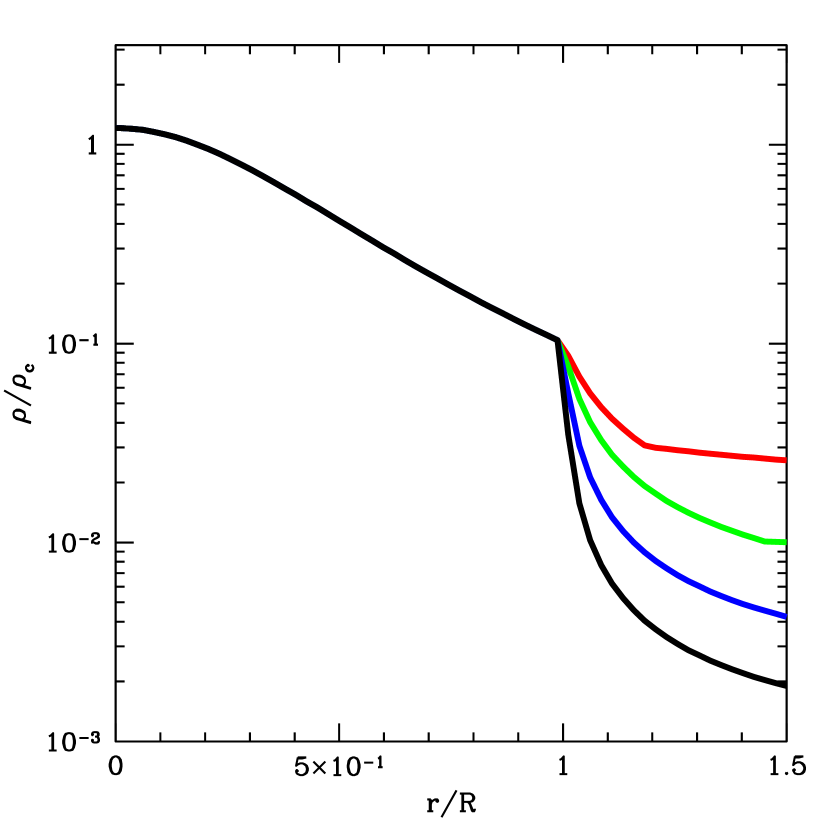
Figure 1.— The initial, unperturbed density profile of the embedded isothermal sphere. The density contrast for each is roughly 50 (black), 25 (blue), 10 (green) and 4 (red). This color scheme will be consistent throughout the other figures.

Table 1External Gas Properties and Damping Rates

Model	$T_{\rm ext}/T$	$\rho_{\rm ext}/\rho_{\rm surf}$	$\tau_{A}$ [$(GM/R^{3})^{-1/2}$]
black	$10^{6}$	0.017	8.5
blue	$300$	0.037	6.5
green	$10$	0.087	4.8
red	$3$	0.22	3.44

Because the thermal gas heating and cooling time, via collisional coupling to dust at high densities (Burke & Hollenbach 1983) and molecular line radiation at low densities (Goldsmith 2001), is short in comparison to the typical oscillation period (on the order of $10^{5}\,{\rm yr}$), the oscillations of dark-starless cores are well modeled with an isothermal equation of state (Keto & Field 2005). In our simulations, we use a barotropic equation of state with an adiabatic index of unity (as opposed to $5/3$, for example), in which case the isothermal evolution is also adiabatic. This allows us to replace the energy equation with a considerably simpler adiabatic constraint. Since the unbounded isothermal gas sphere is unstable, we truncate the solution at a given center-to-edge density contrast ($\rho(R)/\rho_{c}\simeq 12$, not to be confused with the interior/exterior density contrast), producing a stable Bonnor-Ebert sphere solution with radius ($R$) and mass determined by the central density ($\rho_{c}$) and temperature ($T$). This is done by inducing a phase change in the equation of state, i.e.,

$$P=\left\{\begin{array}[]{rl}\rho\frac{kT}{\mu m_{p}}&\mbox{if }\rho\geq\rho(R)\,,\\ \left[\frac{\rho}{\rho(R)}\right]^{\epsilon}\rho(R)\frac{kT}{\mu m_{p}}&\mbox{if }\rho(R)>\rho\geq\beta\rho(R)\frac{T}{T_{\rm ext}}\,,\\ \rho\frac{kT_{\rm ext}}{\mu m_{p}}&\mbox{otherwise}\,,\end{array}\right.$$ (1)

where the intermediate state, with $\beta=0.8$ and $\epsilon=\log(\beta)/\log(\beta T/T_{\rm ext})\ll 1$ chosen to make $P(\rho)$ continuous, is introduced to avoid numerical artifacts at the surface, and $T_{\rm ext}\gg T$. The specific values of $T_{\rm ext}$ that we chose, their corresponding density contrasts and decay timescales, are presented in Table 1. The associated radial density profiles are shown in Figure 1. Note that there is a transition region which distributes the sudden drop in density over many grid zones, though the pressure is continuous (necessarily) and nearly constant outside the surface of the Bonnor-Ebert sphere.

We employ the same three-dimensional, self-gravitating hydrodynamics code as in Broderick et al. (2007) to follow the long term mode evolution. Details regarding the numerical algorithm and specific validation for oscillating gas spheres (in that case a white dwarf) can be found in Broderick & Rathore (2006), and thus will only be briefly summarized here.

The code is a second-order accurate (in space and time) Eulerian finite-difference code, and has been demonstrated to have a low diffusivity. Because the equation of state is barotropic, we use the gradient of the enthalpy instead of the pressure in the Euler equation since this provides better stability in the unperturbed configuration (Broderick & Rathore 2006). The Poisson equation is solved via spectral methods, with boundary conditions set by a multipole expansion of the matter on the computational domain. As described in Broderick et al. (2007), the code was validated for this particular problem finding convergence by a resolution of $128^{3}$ grid zones.

The initial perturbed states are computed in the linear approximation using the standard formalism of adiabatic (which in this case is also isothermal, Keto et al. 2006) stellar oscillations (Cox 1980). The initial conditions of the perturbed gas sphere are then given by the sum of the equilibrium state and the linear perturbation. We employ the same definition for the dimensionless mode amplitude as given in the Appendix of Keto et al. (2006).

Throughout the evolution, the amplitude of a given oscillation mode, denoted by its radial ($n$) and angular ($l$ & $m$) quantum numbers, may be estimated by the explicit integral:

$$A_{nlm}=\omega_{nlm}^{-1}\int{\rm d}^{3}\!x\,\rho\,\mbox{\boldmath$\rm v$}\cdot\mbox{\boldmath$\rm\xi$}_{nlm}^{\dagger}\,,$$ (2)

where $\rm v$ is the gas velocity, $\mbox{\boldmath$\rm\xi$}_{nlm}$ is the mode displacement eigenfunction, $\omega_{nlm}$ is the mode frequency and the dagger denotes Hermitian conjugation.

3. Results & Discussion

In principle, a number of hydrodynamic mechanisms exist by which the oscillations can be damped. In the absence of a coupling to an external medium, these are dominated by nonlinear mode–mode coupling, in which large scale motions excite smaller scale perturbations (Broderick et al. 2007). However, when embedded in a dense external medium it is possible for the mode to damp by exciting motions in the exterior gas. That is, it is possible for the oscillating sphere to act as a transducer, generating sound waves in the external gas which then propagate outward resulting in a net radial energy flux and damping the oscillations.

Generally, this will be a strong function of the density contrast between the interior of the core and the exterior medium. If the external density has a low density, and thus little inertia, outwardly moving sound waves will contain little energy density despite their large amplitude and thus inefficiently damp the mode (as is the case for B68). Similarly, if the exterior medium has a very high density the excited outgoing waves will have small amplitudes, which despite the large gas inertia will again carry away only a small amount of energy. Conversely, when the density contrast is nearly unity, there will be an efficient coupling between the interior and exterior waves, resulting in a rapid flow of energy out of the cloud.

This may be made explicit via the standard three-wave analysis, in which propagating wave solutions for the incident, reflected and transmitted waves on either side of the density continuity are inserted into the continuity and Euler equations, which can subsequently be solved for the reflected and transmitted energy flux. In this idealization the ratio of the reflected to transmitted flux is $4\zeta/(1+\zeta)^{2}$, where

$$\zeta\equiv\rho_{e}c_{s,e}/\rho_{i}c_{s,i}=\sqrt{\rho_{e}/\rho_{i}}\,,$$ (3)

is the ratio of the sonic impedances on either side of the discontinuity (Landau & Lifshitz 1987). As anticipated, when the density of the external gas is comparable to the surface density of the isothermal sphere we may expect efficient transmission of sound waves from the interior to the exterior (i.e., conversion of the oscillation into traveling waves in the exterior), and therefore efficient damping of the pulsations.

This conclusion is also supported by a 1D analysis of the decay of a standing wave confined to a high density region (section A.2), for which the damping rate, $\gamma$ is given by

$$\gamma=\frac{c_{s,i}}{2R}\ln\left(\frac{|1-\zeta|}{1+\zeta}\right)\simeq\frac{c_{s,i}}{R}\zeta\,,$$ (4)

where $c_{s,i}$ is the sound speed in the interior and $R$ is the radius of the high-density region. Thus, as expected lower external densities (corresponding to smaller $\zeta$) have lower damping rates and larger damping timescales. Note that when $\zeta$ is of order unity the wave decays on the sound crossing time of the dense region, as would be expected if, e.g., we were to decompose the standing wave into traveling waves.

More directly applicable to the damping of oscillating gas spheres is the case of the decay of a standing multipolar sound wave in a uniform density sphere, discussed in section A.3. This is distinct from the 1D case in an important way: the oscillation wave vectors are no longer only normal to the boundary. As a consequence, the damping rate is a strong function of not only $\zeta$ but also the multipole structure of the underlying oscillation. In particular, the damping rate for the $l^{\rm th}$ multipole mode is proportional to $\zeta^{2l+3}$ for small $\zeta$ (see, eqs. A23 & B14), which is a very strong function of $\zeta$ for even low $l$! This limiting behavior is also found in semi-analytic calculations (section B) in which the linear oscillation of an isothermal sphere is properly matched to outgoing sound waves in the exterior. The damping timescales (inverse of the damping rates) from both the uniform-sphere approximation and the full linear mode analysis are shown in Figure 2 for the first few multipoles. All of this implies that the damping rates of oscillations of cores embedded in cold molecular regions, where the density contrast between the core and the cloud is near unity, will be much more rapid than those in cores isolated in hot, lower-density regions.

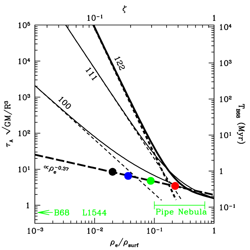
Figure 2.— The damping timescales in units of the dynamical time of the cloud, $(GM/R^{3})^{-1/2}$, as a function of the ratio of the exterior and surface densities. For reference the corresponding damping times in ${\rm M}{\rm yr}$ is shown on the right-hand axis for a cloud similar to Barnard 68. The solid lines show the damping timescale predicted by a linear mode analysis of the isothermal sphere for monopole (011), dipole (111) and quadrupole (122,thick) modes (see the appendices). The asymptotic behavior of the linear mode analysis is shown by the short dashed lines for each, which may be obtained by treating the oscillations of the isothermal sphere as sound waves in a uniform density sphere (see the appendices). The solid circles show the damping timescales measured via numerical simulations, and are colored to match the curves in Figures 1 & 3. Finally, we show a power-law fit to the measured damping timescales, which have a power-law index of $-0.37$, and is considerably flatter than we might have expected (though these represent lower limits upon the decay timescale). For comparison the density contrasts observed in some well known examples are also shown, including those for Barnard 68 ($10^{-5}$), L1544 ($10^{-2}$) and the cores in the Pipe Nebula ($0.1$–$0.7$).

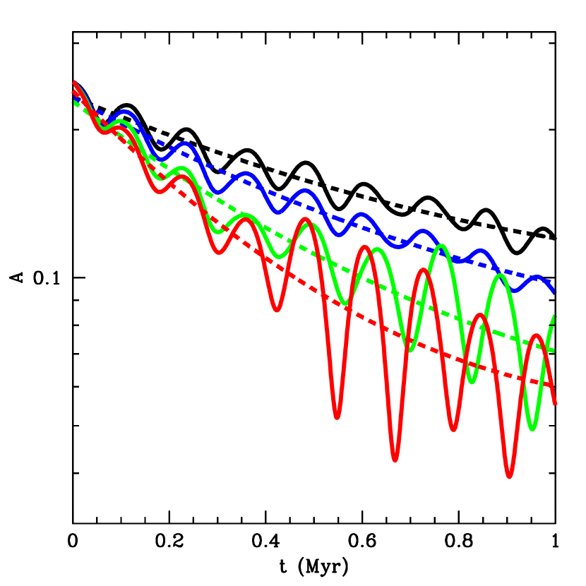
Figure 3.— The mode evolution for various external gas models. The density contrast for each is roughly 50 (black), 25 (blue), 10 (green) and 4 (red), and the lines are colored to match those in Figs. 1 & 2. The decay time for the red curve is 0.43 Myr, compared to 1.05 Myr for the black curve. Quadratic fits for each are shown by the dashed lines. Matching these up to specific models of the mode decay is complicated by (i) the non-linear mode dynamics, and (ii) understanding the energy losses due to traveling waves in the external medium (see the appendices).

However, this is not borne out by numerical simulations of high amplitude oscillations. This can readily be seen by the damping timescales measured via the numerical simulations. Figure 3 shows the evolution of the $n=1$, $l=2$, $m=2$ mode discussed in Broderick et al. (2007). In all cases the initial amplitude was 0.25, and the evolution of the mode well fit by a decaying exponential. Oscillations on isothermal cores embedded in higher density regions did indeed damp more rapidly, as is apparent in the figure. Explicit values of the decay timescale are presented in Table 1, though as in Broderick et al. (2007) these should be seen as lower limits only due to coupling in the artificial atmosphere. These are plotted as a function of the surface density contrast in Figure 2, shown by the colored filled circles. For reference, we show the approximate surface density contrasts of Barnard 68 (Alves, Lada, & Lada 2001), L1544 (Ward-Thompson, Motte, & Andre 1999) and typical for cores in the Pipe Nebula (Lada et al. 2008). While there is a clear power-law dependence of the damping timescale upon $\zeta$, with $\tau_{A}\propto(\rho_{e}/\rho_{i})^{-0.37}$ this dependence is considerably weaker than that predicted by the linear analysis ($\tau_{A}\propto(\rho_{e}/\rho_{i})^{-3.5}$).

This disparity may be understood in terms of the relative importance of the excitation of sound waves in the exterior medium to the damping of the oscillations. In particular, it is notable that the numerically measured damping timescales are always less, and for most surface density contrasts considerably so, than those implied by the linearized analysis of external sound wave excitation. This is true even with low amplitude oscillations (e.g., $A=10^{-4}$, for which the damping timescale is roughly a factor of 3 larger than for $A=0.25$ ) and thus is likely due to mode coupling in the transition region immediately outside the cloud (seen in Fig. 1 immediately outside $r/R=1$ as the region of rapidly decreasing density). Within this region the densities are all within a single order of magnitude despite their very different asymptotic densities at infinity (which differ by many orders of magnitude). As a consequence, the damping rates inferred from the isolated isothermal spheres are only a weak function of the properties of the external medium. Thus, even for surface density contrasts on the order of $1/4$, the decay timescale for the quadrupolar oscillation is still larger than $4\times 10^{5}\,{\rm yr}$, corresponding to many oscillations and comparable to the inferred lifetimes of globules.

4. Conclusions

Despite the expectations of the linear mode analysis of the embedded isothermal sphere, the damping timescale of large-amplitude oscillations of embedded Bonnor-Ebert spheres is only a weak function of the density of the external medium. This is a result of the dominance of nonlinear mode–mode coupling in the damping of large oscillations. Even in cold molecular environments, the quadrupolar oscillation discussed in Keto et al. (2006) and Broderick et al. (2007) has a lifetime of at least $0.4\,{\rm M}{\rm yr}$, and is thus comparable to the inferred lifetimes of globules (Lada et al. 2008). This suggests that globules supporting large-amplitude oscillations may be common even in these environments.

The presence of large-amplitude oscillations on starless cores has a number of consequences for the physical interpretation of observations of starless cores (Keto et al. 2006; Broderick et al. 2007). Necessarily they would imply that starless cores are stable objects, existing for many sound-crossing times. In addition, the signatures of collapse, expansion and rotation in observations of self-absorbed molecular lines (e.g., CS) are degenerate with molecular line profiles produced by oscillating globules (see, e.g., figure 6 of  Broderick et al. 2007). Consequently, it may be difficult to determine the true dynamical nature of motions in a given globule or dense core from self-absorbed, molecular-line profiles alone. This suggests that studies of such profiles in dense cores may be of only statistical value in determining the general status of motions in dense core populations.

Appendix A Damping of an Oscillating Cavity

We will first review some basic facts about sound waves in uniform media. Beginning in subsection A.2 we will discuss the evolution of a one-dimensional standing sound wave as a result of the excitation of waves in the external medium. In subsection A.3 we discuss the application to oscillating uniform density spheres, and treat the full linearized mode analysis of isothermal spheres in section B.

A.1. Equations of Motion

The governing equations are the linearized continuity and the Euler equations:

$$\dot{\rho^{\prime}}+\mbox{\boldmath$\rm\nabla$}\cdot\rho_{0}\mbox{\boldmath$\rm\delta v$} =0\,,$$

$$\dot{\mbox{\boldmath$\rm\delta v$}}+\frac{c_{s}^{2}}{\rho_{0}}\mbox{\boldmath$\rm\nabla$}\rho^{\prime} =0\,,$$ (A1)

where $\rho_{0}$ and $c_{s}$ are the unperturbed density and sound speed, respectively, $\rho^{\prime}$ is the Eulerian perturbation in the density and $\rm\delta v$ is the Lagrangian perturbation in the velocity (which is identical to the Eulerian perturbation since the initial velocity field is assumed to vanish). These may be combined in the normal way to produce the wave equation

$$\ddot{\rho^{\prime}}-c_{s}^{2}\nabla^{2}\rho^{\prime}=0\,,$$ (A2)

where we have assumed that the background density is uniform. Solutions will generally obey the dispersion relation $k^{2}=c_{s}^{2}\omega^{2}$, and may then be inserted into the Euler equation to obtain the associated velocity perturbation.

A.2. Decay of a One-Dimensional Sound Wave

We will consider the decay of a sound wave traveling inside of a uniform high density region (called the interior and denoted by sub-script $i$’s) surrounded by a uniform low density region (called the exterior and denoted by sub-script $e$’s). The interior wave oscillation is given by

$$\rho^{\prime}_{i}=A_{i}\rho_{i}\sin(k_{i}x){\rm e}^{-i\omega t}\quad{\rm and}\quad\delta v^{x}_{i}=-iA_{i}c_{s,i}\cos(k_{i}x){\rm e}^{-i\omega t}\,.$$ (A3)

The exterior waves are outgoing, and we will focus upon the boundary condition at the $+R$ boundary. At this point the exterior sound wave is given by

$$\rho^{\prime}_{e}=A_{e}\rho_{e}{\rm e}^{ik_{e}x-i\omega t}\quad{\rm and}\quad\delta v^{x}_{e}=A_{e}c_{s,e}{\rm e}^{ik_{e}x-i\omega t}\,.$$ (A4)

At the interface we require (i) pressure equilibrium and (ii) continuity of the displacement and hence velocity. Since we have assumed the $\rho_{i}$ and $\rho_{e}$ are constant, the first condition is simply $\rho^{\prime}_{i}c_{s,i}^{2}=\rho^{\prime}_{e}c_{s,e}^{2}$. The second is trivially $\delta v^{x}_{i}=\delta v^{x}_{e}$. Thus

$$A_{i}\rho_{i}c_{s,i}^{2}\sin(k_{i}R){\rm e}^{-i\omega t}=A_{e}\rho_{e}{\rm e}^{ik_{e}R-i\omega t}\quad{\rm and}\quad-iA_{i}c_{s,i}\cos(k_{i}R){\rm e}^{-i\omega t}=A_{e}c_{s,e}{\rm e}^{ik_{e}R-i\omega t}\,,$$ (A5)

give two complex equations from which we may determine $A_{e}$ and $\omega$ as functions of $A_{i}$ and the background fluid quantities (note that $k_{i}=\omega/c_{s,i}$ and $k_{e}=\omega/c_{s,e}$ by the dispersion relations in each region). In particular, note that by taking the ratio of the two equations we find

$$\tan(k_{i}R)=-i\zeta\,,$$ (A6)

where $\zeta\equiv\rho_{e}c_{s,e}/\rho_{i}c_{s,i}=\sqrt{\rho_{e}/\rho_{i}}$ is the ratio of the exterior and interior sonic impedances. Generally this may be solved to find that $k_{i}R=n\pi+(i/2)\ln\left[|1-\zeta|/(1+\zeta)\right]$, however we will solve this explicitly in the $\zeta\ll 1$ limit to illustrate how we will do this for spherical geometries later.

Let us begin by assuming that the damping rate is small. Specifically, let us assume that $\omega_{0}\equiv\Re(\omega)$ is much larger than $\gamma\equiv-\Im(\omega)$. Then we may Taylor expand the left-hand side of eq. (A6) around $\gamma=0$:

$$\tan(k_{i}R)=\tan\left(\frac{\omega_{0}R}{c_{s,i}}\right)-\left.\frac{\partial\tan}{\partial\omega}\right|_{\omega=\omega_{0}}i\gamma+\dots=0-i\zeta\,,$$ (A7)

and thus, equating real and imaginary parts

$$\tan\left(\frac{\omega_{0}R}{c_{s,i}}\right)=0\quad\Rightarrow\quad\omega_{0}=n\pi\frac{c_{s,i}}{R}$$ (A8)

and

$$\left[1+\tan^{2}\left(\frac{\omega_{0}R}{c_{s,i}}\right)\right]\frac{\gamma R}{c_{s,i}}=\zeta\quad\Rightarrow\quad\gamma=\frac{c_{s,i}}{R}\zeta\,.$$ (A9)

We may in principle then insert this into eq. (A6) to obtain the relationship between $A_{i}$ and $A_{e}$. However, we will be concerned with only the damping rate here.

A.3. Damping Timescale of an Oscillating Sphere

In the previous section we discussed the simple problem of the damping of a one-dimensional wave due to the excitation of outgoing exterior sound waves. In this section we will address the more relevant problem of the damping timescale of multipolar oscillations on a sphere. While generally we would use the linearized analysis of the oscillating isothermal sphere, here we will limit ourselves to the spherical analog of the previous section: a sound wave in a uniform density sphere surrounded by a uniform density exterior.

Before we can discuss the excitation of sound waves outside of an oscillating sphere we must first determine the explicit form of these waves. We do this by separating the radial and angular dependencies using spherical harmonics (primarily because these were used in determining the mode spectrum of the isothermal sphere). That is, we let $\rho^{\prime}={\rm e}^{-i\omega t}\mathcal{R}(r)Y_{lm}(\hat{\mbox{\boldmath$\rm r$}})$, and insert this into equation (A2), producing

$$\frac{1}{r}\frac{\partial^{2}}{\partial r^{2}}r\mathcal{R}-\frac{l(l+1)}{r^{2}}\mathcal{R}+k^{2}\mathcal{R}=0\,,$$ (A10)

where $k\equiv\omega/c_{s}$. The general solutions of this equation are simply the spherical Bessel functions:

$$\mathcal{R}(r)=aj_{l}\left(kr\right)+bn_{l}\left(kr\right)\,.$$ (A11)

However, we must still separate the inward and outward traveling waves. This naturally occurs if we consider spherical Bessel functions of the 3rd kind, which are necessarily simply linear combinations of spherical Bessel functions of the 1st and 2nd kind ($j_{l}$ and $n_{l}$, respectively):

$$h_{l}^{(1,2)}(z)\equiv j_{l}(z)\pm in_{l}(z)\propto\frac{{\rm e}^{\pm iz}}{z^{l+1}}\,.$$ (A12)

Outwardly directed waves are given by $h_{l}^{(1)}(z)$ and inwardly directed waves are given by $h_{l}^{(2)}(z)$. In terms of this the density perturbation of the exterior sound waves associated with the $l,m$ multipole is

$$\rho^{\prime}_{e}=A_{e}\rho_{e}{\rm e}^{-i\omega t}h_{l}^{(1)}(k_{e}r)Y_{lm}(\hat{\mbox{\boldmath$\rm r$}})\,,$$ (A13)

where $A_{e}$ is a dimensionless wave amplitude. For $l=0$ this results in the standard spherical wave solutions, $\propto{\rm e}^{\pm ikr}/r$. The velocity perturbation may be determined via the linearized Euler equation:

$$\delta v^{r}_{e}=-i\frac{c_{s}^{2}}{\omega\rho_{e}}\frac{\partial\rho^{\prime}_{e}}{\partial r}=-iA_{e}c_{s,e}{\rm e}^{-i\omega t}\frac{\partial h_{l}^{(1)}}{\partial z_{e}}(z_{e})Y_{lm}(\hat{\mbox{\boldmath$\rm r$}})\,,$$ (A14)

where here and henceforth we have defined $z_{e}\equiv k_{e}r$ for convenience. In contrast, the interior wave must be regular at the origin, and is given by

$$\rho^{\prime}_{i}=A_{i}\rho_{i}{\rm e}^{-i\omega t}j_{l}(k_{i}r)Y_{lm}(\hat{\mbox{\boldmath$\rm r$}})\quad{\rm and}\quad\delta v^{r}_{i}=-iA_{i}c_{s,i}{\rm e}^{-i\omega t}\frac{\partial j_{l}}{\partial z_{i}}(z_{i})Y_{lm}(\hat{\mbox{\boldmath$\rm r$}})\,,$$ (A15)

where $z_{i}\equiv k_{i}r=z_{e}/\zeta$.

At the interface we again require pressure equilibrium and continuity in the radial velocity:

$$A_{i}\rho_{i}c_{s,i}^{2}{\rm e}^{-i\omega t}j_{l}(k_{i}r)Y_{lm}(\hat{\mbox{\boldmath$\rm r$}})=A_{e}\rho_{e}c_{s,e}^{2}{\rm e}^{-i\omega t}h_{l}^{(1)}(k_{e}r)Y_{lm}(\hat{\mbox{\boldmath$\rm r$}})$$ (A16)

and

$$-iA_{i}c_{s,i}{\rm e}^{-i\omega t}\frac{\partial j_{l}}{\partial z_{i}}(z_{i})Y_{lm}(\hat{\mbox{\boldmath$\rm r$}})\,.=-ic_{s,e}{\rm e}^{-i\omega t}\frac{\partial h_{l}^{(1)}}{\partial z_{e}}(z_{e})Y_{lm}(\hat{\mbox{\boldmath$\rm r$}})$$ (A17)

As before, together with $\omega=k_{i}/c_{s,i}=k_{e}/c_{s,e}$ and $z_{e}=\zeta z_{i}$, these are sufficient to determine $A_{e}$ and $\omega$. In particular, these imply

$$\frac{\partial\ln j_{l}}{\partial z_{i}}(z_{i})=\frac{1}{\zeta}\frac{\partial\ln h^{(1)}_{l}}{\partial z_{e}}(z_{e})$$ (A18)

The right-hand side may be simplified in the $z_{e}\ll 1$ limit. Since $z_{i}$ is typically of order unity, this implies that $\zeta\ll 1$. In this regime, to leading order in small $z_{e}$,

$$\frac{1}{\zeta}\frac{\partial\ln h^{(1)}_{l}}{\partial z_{e}}(z_{e})\simeq-\frac{l+1}{z}+i\frac{z_{e}^{2l}}{\left[(2l-1)!!\right]^{2}}\,,$$ (A19)

where $(2l-1)!!=(2l-1)\cdot(2l-3)\cdots 5\cdot 3\cdot 1$.

Again let us begin with the ansatz that the damping rate is small for small $\zeta$. In which case

$$\left.\frac{\partial\ln j_{l}}{\partial z_{i}}\right|_{\omega_{0}}-\left.\frac{\partial^{2}\ln j_{l}}{\partial z_{i}^{2}}\right|_{\omega_{0}}i\frac{\gamma R}{c_{s,i}}+\dots=-\frac{l+1}{\zeta^{2}z_{i}}+i\frac{\zeta^{2l-1}z_{i}^{2l}}{\left[(2l-1)!!\right]^{2}}\,,$$ (A20)

and thus

$$\displaystyle\left.\frac{\partial\ln j_{l}}{\partial z_{i}}\right|_{\omega_{0}}=\left[\frac{j_{l-1}(z_{i})}{j_{l}(z_{i})}-\frac{l+1}{z_{i}}\right]_{\omega_{0}}=-\frac{l+1}{\zeta^{2}z_{i}}$$

$$\displaystyle\qquad\qquad\qquad\qquad\qquad\quad\Rightarrow\quad\frac{j_{l-1}(z_{i})}{j_{l}(z_{i})}\simeq-\frac{l+1}{\zeta^{2}z_{i}}\quad{\rm and}\quad\omega_{0}\simeq\frac{c_{s,i}}{R}\mathcal{Z}_{nl}$$ (A21)

where $\mathcal{Z}_{nl}$ is the $n^{\rm th}$ root of $j_{l}(z)$. With

$$\left.\frac{\partial^{2}\ln j_{l}}{\partial z_{i}^{2}}\right|_{\omega_{0}}\simeq-\left[\frac{j_{l-1}(z_{i})}{j_{l}(z_{i})}\right]^{2}\simeq-\frac{(l+1)^{2}}{\zeta^{4}\mathcal{Z}_{nl}^{2}}\,,$$ (A22)

(where we used the fact that $\zeta\ll 1$) we find

$$\gamma=\frac{c_{s,i}}{R}\frac{\zeta^{2l+3}\mathcal{Z}_{nl}^{2l+2}}{(l+1)^{2}\left[(2l-1)!!\right]^{2}}\,.$$ (A23)

We note that this is quite different than the one-dimensional case. In particular, the decay rate decreases rapidly with decreasing $\zeta$, and is a strong function of $l$, with higher multipoles decaying considerably more rapidly than lower multipoles. This is a consequence of our assumption that not just $\zeta\ll 1$, but $\zeta z_{i}\ll 1$ (justified in our case), which implies that $\lambda_{e}\gg R$. That is, the exterior propagating sound wave necessarily knows that the geometry is converging, with higher multipoles converging more rapidly.

We should also emphasize that the scaling of the damping rate, $\gamma$, with $\zeta$ is dependent primarily upon the structure of the traveling sound waves in the exterior. Rather, the properties of the interior perturbation are encoded in the definition of the $\mathcal{Z}_{nl}$, and thus the normalization. Therefore, the damping rates associated with the linearized perturbations of the pressure-supported isothermal sphere (Bonnor-Ebert sphere) should be quite similar, differing only in the particular values of $\mathcal{Z}_{nl}\simeq 2\pi R/\lambda_{i}$. Indeed, in the next section we find this to be the case.

Appendix B Damping of Oscillating Isothermal Spheres in the Linear Regime

The rather surprisingly strong scaling of the damping timescale with the density contrast motivates a more careful analysis of the damping rates of a self-gravitating, pressure supported isothermal sphere. The mode analysis of an isothermal sphere has been treated in considerable detail elsewhere (e.g., Cox 1980; Keto et al. 2006) and thus we summarize it only briefly here. The perturbed quantities are most conveniently described by the Dziembowski variables (Dziembowski 1971)

$$\mbox{\boldmath$\rm\eta$}(\mbox{\boldmath$\rm r$})=\left(\frac{\delta r}{r},\frac{P^{\prime}+\rho_{0}\psi^{\prime}}{\rho_{0}gr},\frac{\psi^{\prime}}{gr},\frac{1}{g}\frac{\partial\psi^{\prime}}{\partial r}\right)\,,$$ (B1)

which may be separated into radial and angular parts, $\eta_{i}(\mbox{\boldmath$\rm r$})=\eta_{i}(r){\rm e}^{-i\omega t}Y_{lm}(\hat{\mbox{\boldmath$\rm r$}})$. In terms of these, the linearized hydrodynamic equations are given by

$$r\frac{\partial\eta_{1}}{\partial r}=(V-3)\eta_{1}+\left[\frac{l(l+1)}{\sigma^{2}C}-V\right]\eta_{2}+V\eta_{3}$$ (B2a)

$$r\frac{\partial\eta_{2}}{\partial r}=\sigma^{2}C\eta_{1}+(1-U)\eta_{2}$$ (B2b)

$$r\frac{\partial\eta_{3}}{\partial r}=(1-U)\eta_{3}+\eta_{4}$$ (B2c)

$$r\frac{\partial\eta_{4}}{\partial r}=UV\eta_{2}+\left[l(l+1)-UV\right]\eta_{3}-U\eta_{4}\,,$$ (B2d)

where

$$U\equiv\frac{\partial\ln r^{2}g}{\partial\ln r}\,,\quad V\equiv-\frac{\partial\ln P_{0}}{\partial\ln r}\,,\quad C\equiv-\frac{GM}{r^{2}g}\left(\frac{r}{R}\right)^{3}\,,\quad\sigma^{2}\equiv\frac{R^{3}\omega^{2}}{GM}\,,$$ (B3)

are functions of the background equilibrium configuration. These are solved subject to a normalization condition $\eta_{1}(R)=1$ and the inner boundary conditions:

$$\sigma^{2}C\eta_{1}\big{|}_{r=0}=l\eta_{2}\big{|}_{r=0}\qquad{\rm and}\qquad\eta_{4}\big{|}_{r=0}=l\eta_{3}\big{|}_{r=0}\,,$$ (B4)

arising from regularity at the origin. A third boundary condition is a result from the continuity of the gravitational potential at the sphere’s surface,

$$\eta_{4}\big{|}_{r=R}=-(l+1)\eta_{3}\big{|}_{r=R}\,.$$ (B5)

If the exterior density vanishes, as was assumed in Keto et al. (2006), the final boundary condition is given by requiring that the Lagrangian pressure perturbation,

$$\delta P=P^{\prime}+\mbox{\boldmath$\rm\delta r$}\cdot\mbox{\boldmath$\rm\nabla$}P_{0}=\rho_{0}gr\left(\eta_{2}-\eta_{3}-\eta_{1}\right)=0\,.$$ (B6)

However, we now properly match this onto the outgoing multipolar wave solutions described in section A.3. Namely,

$$\delta P=\rho^{\prime}_{e}c_{s,e}^{2}=A_{e}\rho_{e}h^{(1)}_{l}(z_{e})\,,$$ (B7)

subject to

$$\delta r=\eta_{1}R=\frac{c_{s,e}^{2}}{\omega^{2}\rho_{e}}\frac{\partial\rho^{\prime}_{e}}{\partial r}=A_{e}\frac{c_{s,e}}{\omega}\frac{\partial h^{(1)}_{l}}{\partial z_{e}}\,.$$ (B8)

Therefore,

$$\left.\eta_{2}-\eta_{3}-\eta_{1}\right|_{r=R}=\left.\eta_{1}\frac{h^{(1)}}{\partial h^{(1)}/\partial z_{e}}\frac{\rho_{e}c_{s,e}\omega}{\rho_{0}g}\right|_{r=R}\,.$$ (B9)

As before we assume that the damping rate is small, set $\omega=\omega_{0}-i\gamma$ and employ the boundary condition

$$\left.\eta_{2}-\eta_{3}-\eta_{1}\right|_{r=R}=\Re\left[\eta_{1}\frac{h^{(1)}}{\partial h^{(1)}/\partial z_{e}}\frac{\rho_{e}c_{s,e}\omega}{\rho_{0}g}\right]_{r=R,\omega=\omega_{0}}\,.$$ (B10)

The damping rate is then estimated by

$$\gamma=-\Im\left[\eta_{1}\frac{h^{(1)}}{\partial h^{(1)}/\partial z_{e}}\frac{\rho_{e}c_{s,e}\omega}{\rho_{0}g}\right]_{r=R,\omega=\omega_{0}}\bigg{/}\left.\frac{\partial(\eta_{2}-\eta_{3})}{\partial\omega}\right|_{r=R}\,,$$ (B11)

where we used the fact that $\partial\eta_{1}/\partial\omega=0$ by the normalization condition. In practice $\partial(\eta_{2}-\eta_{3})/\partial\omega$ is evaluated by solving the eigenvalue problem for the $\eta_{i}$ and $\sigma^{2}$ using

$$\left.\eta_{2}-\eta_{3}-\eta_{1}\right|_{r=R}=\alpha\Re\left[\eta_{1}\frac{h^{(1)}}{\partial h^{(1)}/\partial z_{e}}\frac{\rho_{e}c_{s,e}\omega}{\rho_{0}g}\right]_{r=R,\omega=\omega_{0}}\bigg{/}\left.\frac{\partial(\eta_{2}-\eta_{3})}{\partial\omega}\right|_{r=R}\,,$$ (B12)

and setting

$$\frac{\partial(\eta_{2}-\eta_{3})}{\partial\omega}=\frac{\partial(\eta_{2}-\eta_{3})/\partial\alpha}{\partial\omega/\partial\alpha}\,.$$ (B13)

This amounts to finding $\partial(\eta_{2}-\eta_{3})/\partial\omega$ holding the other boundary conditions constant.

The results of this procedure are explicitly shown in Figure 2. Of particular note is that the intuition obtained from the analysis of sound waves in a uniform density sphere is borne out in the low $\rho_{e}/\rho_{0}(R)$ limit, for which

$$\gamma\propto\left(\frac{\rho_{e}}{\rho_{0}(R)}\right)^{(2l+3)/2}=\zeta^{2l+3}\,.$$ (B14)

References

- Aguti et al. (2007) Aguti, E.D., Lada, C.J., Bergin, E.A., Alves, J.F., Birkinshaw, M., 2007, ApJ, 665, 457
- Alves, Lada, & Lada (2001) Alves, J., Lada, C., & Lada, E. 2001, Nature, 409, 159
- Bacmann et al. (2000) Bacmann, A., Andre, A.P., Puget, J.-L., Abergel, A., Bontemps, S., & Ward-Thompson, D. 2000, å, 361, 555
- Benson & Myers (1989) Benson, P., & Myers, P. 1989, ApJS, 307, 337
- Bergin & Tafalla (2007) Bergin, E. A., & Tafalla, M., 2007, ARA&A, 45, 339
- Bonnor (1956) Bonnor, W., 1956, MNRAS, 116, 351
- Broderick et al. (2007) Broderick, A. E., Keto E., Lada, C. J. & Narayan, R., 2007, ApJ, 000, 000
- Broderick & Rathore (2006) Broderick, A. E. and Rathore, Y., 2006, MNRAS, 372, 923
- Burke & Hollenbach (1983) Burke, J. R. & Hollenbach, D. J., 1983, ApJ, 265, 223
- Cox (1980) Cox, J.P., 1980, Theory of Stellar Pulsations, Princeton University Press: Princeton
- Crapsi et al. (2004) Crapsi, A., Caselli, P., Walmsley, C.M., Tafalla, M., Lee, C.W., Bourke, T.L., Myers, P.C., 2004, å, 420, 957
- Dziembowski (1971) Dziembowski, W., 1971 Acta Astron., 21, 289
- Evans et al. (2001) Evans, N., Rawlings J., Shirley, Y., & Mundy, L. 2001, ApJ, 557, 193
- Goldsmith (2001) Goldsmith, P., 2001, ApJ, 557, 736
- Goldsmith (2008) Goldsmith, P. et al., 2008, arXiv:0802.2206v1 [astro-ph]
- Gregersen et al. (1997) Gregersen, E., Evans, N., Zhou, S., Choi, M., 1997, ApJ, 484, 256
- Gregersen & Evans (2000) Gregersen, E., Evans, N., 2000, ApJ, 538, 260
- Keto et al. (2006) Keto, E., Broderick, A.E., Lada, C.J. & Narayan, R., 2006, ApJ, 652, 1366
- Keto et al. (2004) Keto, E., Rybicki, G., Bergin, E., Plume, R., 2004, ApJ, 613, 355
- Keto & Field (2005) Keto, E. & Field, G., 2005, ApJ, 635, 1151
- Lada et al. (2003) Lada, C., Bergin, E., Alves, J., Huard, T., 2003, ApJ, 586, 286
- Lada et al. (2008) Lada, C. et al., 2008, ApJin publication
- Landau & Lifshitz (1987) Landau, L.D. & Lifshitz, E.M., 1987, Course of Theoretical Physics, Vol. 6, 2nd Ed., Butterworth-Heinemann: Oxford
- Launhardt et al. (1998) Launhardt, R., Evans, N., Wang, Y., Clemens, D., Henning, T., Yun, J., 1998, ApJS, 119, 59
- Lee, Bergin & Evans (2004) Lee, J., Bergin, E., Evans, N., 2004, ApJ, 617, 360
- Lee & Myers (1999) Lee, C.W. & Myers, P.C. 1999, ApJS, 123, 233
- Lee, Myers, & Plume (2004) Lee, C.W., Myers, P., Plume, R., 2004, ApJS, 153, 253
- Lee, Myers, & Tafalla (1999) Lee, C., Myers, P., & Tafalla, M. 1999, ApJ, 576, 788
- Lee, Myers, & Tafalla (2001) Lee, C., Myers, P., & Tafalla, M. 2001, ApJS, 136, 703
- Myers & Benson (1983) Myers, P., & Benson, P. 1983, ApJ, 266, 309
- Myers, Linke, & Benson (1983) Myers, P., Linke, R., & Benson, P. 1983, ApJ, 264, 517
- Shirley et al. (2000) Shirley, Y., Evans, N., Rawlings, J., Gregersen, E., 2000, ApJS, 131, 249
- Shirely et al. (2002) Shirely, Y. L., Evans, N. J., Rawlings, J. M. C., 2002, ApJ, 575, 337
- Sohn et al. (2004) Sohn, J., Lee, C., Lee, H., Park, Y-S., Myers, P., Lee, Y., Tafalla, M., 2005, JKAS, 37, 261
- Tafalla et al. (1998) Tafalla, M., Mardones, D., Myers, P. C., Caselli, P., Bachiller, R. & Benson, P. J., 1998, ApJ, 504, 900
- Tafalla et al. (2002) Tafalla, M., Myers, P., Caselli, P., Walmsley, C. & Comito, C., 2002, ApJ, 569, 815
- Tafalla et al. (2004) Tafalla, M., Myers, P. C., Caselli, P., Walmsley, C. M., 2004, å, 416, 191
- Wang et al. (1995) Wang, Y., Evans, N., Shudong, Z., Clemens, D., 1995, ApJ, 454, 742
- Ward-Thompson, Motte, & Andre (1999) Ward-Thompson, D., Motte, F. & Andre, P. 1999, MNRAS, 305, 143
- Ward-Thompson et al. (1994) Ward-Thompson, D., Scott, P., Hills, R., & Andre, P. 1994, MNRAS, 268, 274
- Williams et al. (1999) Williams, J., Myers, P., Wilner, D., Di Francesco, J., 1999, ApJ, 513, L61
- Young et al. (2003) Young, C., Shirley, Y., Evans, N., Rawlings, J., 2003, ApJS, 145, 111
- Zhou et al. (1994) Zhou, S., Evans, N., Wang, Y., Peng, R., Lo, K., 1994, ApJ, 433, 131