Supermassive Black Holes and Their Environments

Abstract

We make use of the first high–resolution hydrodynamic simulations of structure formation which self-consistently follows the build up of supermassive black holes introduced in Di Matteo et al. (2007) to investigate the relation between black holes (BH), host halo and large–scale environment. There are well–defined relations between halo and black hole masses and between the activities of galactic nuclei and halo masses at low redshifts. A large fraction of black holes forms anti–hierarchically, with a higher ratio of black hole to halo mass at high than at low redshifts. At $z=1$, we predict group environments (regions of enhanced local density) to contain the highest mass and most active (albeit with a large scatter) BHs while the rest of the BH population to be spread over all densities from groups to filaments and voids. Density dependencies are more pronounced at high rather than low redshift. These results are consistent with the idea that gas rich mergers are likely the main regulator of quasar activity. We find star formation to be a somewhat stronger and tighter function of local density than BH activity, indicating some difference in the triggering of the latter versus the former. There exists a large number of low–mass black holes, growing slowly predominantly through accretion, which extends all the way into the most underdense regions, i.e. in voids.

1 Introduction

Remnant supermassive black holes (BHs) from an early quasar phase are now being found ubiquitously in the centers of local galaxies. Even more remarkably, a number of tight correlations have been discovered between the black hole mass $m_{\rm BH}$ and properties of the host, such as the bulge mass, $m_{\rm bulge}$, or K-band luminosity or its velocity dispersion, $\sigma$ (e.g.;Ferrarese and Merritt 2000, Gebhardt et al. 2000, Marconi & Hunt 2003, Haring & Rix 2004). These relations demonstrate a strong link between BHs and galaxy formation and have thus motivated a large theoretical effort to address their origin and evolution (e.g., Kauffmann & Haehnelt 2000, Adams et al. 2001, Di Matteo et al. 2003, Hatziminaoglou et al. 2003, Hopkins et al. 2005, Bower et al. 2006, Croton et al. 2006, Marulli et al. 2007 ; for a review of semi–analytical models especially Baugh 2006).

Recent ultra-deep Chandra X-ray observations of submillimeter galaxies (SMGs; Alexander et al. 2005) imply that the time of rapid black hole growth is related to activity at sites of intensive star formation and hence to massive flows of gas at the center of galaxies. SMGs are indeed roughly coeval with the peak of the quasar phase. UV images from the Hubble Space Telescope show that a considerable fraction of SMGs are undergoing a major merger (Conselice et al. 2003, Pope et al. 2005). In the local universe, ultraluminous infrared (ULIRG) systems associated with merger driven starburst activity have now been directly shown to be associated with black hole growth (Komossa et al. 2003), supporting the same picture for a link between quasar activity and merger induced starbursts in galaxies and formation of bulges.

Quasars with inferred black hole masses of around $10^{9}$ M_⊙ at redshifts of $z\sim 6$ (Fan et al. 2003, Jiang et al. 2007, Kurk et al. 2007) have been discovered. In view of our standard picture of structure formation, the implications from the local $m_{\rm BH}$–$\sigma$ and the association of black hole fuelling with a major merger and a starburst, it is challenging to understand the presence of such massive objects at $z\sim 6$. Outstanding questions remain as to where and how these first BH form and what their descendants in our local universe are. Furthermore, it is now known that the space density of low luminosity X–ray selected AGN peaks at lower redshifts than that of high luminosity ones (e.g. Steffen et al. 2003, Ueda et al. 2003, Hasinger et al. 2005), an effect called “cosmic downsizing”. If the build–up of galaxies proceeds from smaller ones to larger ones, it is hard to explain why the bulk of the mass in the largest black holes and brightest AGN/quasars was acquired first, whereas today the lower mass black holes are being assembled.

These and other lines of evidence firmly demonstrate that even though the growth of black holes is intimately linked to the formation and evolution of galaxies, it is not directly linked to the growth of the halo mass function. Naturally, the growth of black holes and galaxies has to be addressed in the framework of the standard $\Lambda$ cold dark matter ($\Lambda$CDM) cosmology. In that context, semi–analytical models have been developped (e.g. Cattaneo et al. 1999, Kauffmann & Haehnelt 2000, Granato et al. 2001, Wyithe & Loeb 2003), which at first linked black hole directly to the growth of dark matter halos and quasar activity to major mergers. The latest generation of these models has started to incorporate AGN feedback, which truncates ongoing star formation and suppresses cooling in more massive halos (see, e.g; Granato et al. 2004, Monaco & Fontanot 2005, Bower et al. 2006, Croton et al. 2006, De Lucia et al. 2006, Malbon et al. 2007). Such models often suggest that the fundamental relations between galaxy structure and black holes may arise if feedback energy expels (in the form of strong outflows) the nearby gas and shuts down the accretion phase (Ciotti & Ostriker 1997, Silk & Rees 1998, Fabian 1999, Wyithe & Loeb 2003). This picture has now been confirmed in studies employing detailed galaxy simulations (Di Matteo et al. 2005; Robertson et al. 2006; Di Matteo et al. 2007).

The coupling of mergers, star formation with black hole growth/quasar activity in the context of galaxy evolution is difficult to treat on the basis of analytical estimates alone. Such methods unavoidably neglect the dynamics of quasar evolution in galaxies, and they cannot predict time–dependent effects such as the characteristic lifetime of the accretion phase prior to its self-termination, the available fueling rates driven by gas inflows that regulate the black hole accretion, and their dependence on the environment.

In this paper we present a detailed study of the cosmological evolution of the demographics of supermassive black holes as a function of their local environment. We use the first full hydrodynamical high–resolution simulation of a cosmological volume that incorporates black hole growth and associated feedback self-consistently (Di Matteo et al. 2007, Sijacki et al. 2007), based on the methodology developed and explored in hydrodynamical simulation of galaxy mergers (Di Matteo, Springel & Hernquist 2005; Springel, Di Matteo & Hernquist 2005). Using a direct cosmological SPH simulation, besides treating the hierarchical assembly of black holes and their haloes, allows us to consider the physical conditions of the gas inflows that drive star formation and lead to the growth of the central black holes in galaxies as well as their interaction with associated feedback processes.

In Di Matteo et al. (2007), we discussed some promising results from this simulation method, which include its ability to reproduce the local value of the black hole mass density, $\rho_{BH}$, and its extrapolation to higher redshift ($z<2.5$), as well as a peak in the global black hole accretion rate history at $z\sim 2-3$, the expected peak of the quasar phase, and a sharp drop at higher redshifts (see also Sijacki et al. 2007). These trends are consistent with the general picture, in which gas is available for star formation and eventually gets to the central regions to ignite the quasar activity in major mergers. In addition, the locations of our cosmological galaxies and black holes agree very well with the local $m_{\rm BH}-m_{\sigma}$ and $m_{\rm BH}-m_{*}$ relations over a very large dynamic range and predict an evolution consistent with recent observational studies (Woo et al. 2006, Shields et al. 2006, Peng et al. 2006). Here, we carry out a detailed study of the local environments of black holes as a function of redshift. We will look at the relations between black hole hole mass and accretion rate for BHs in the simulation with halo mass, relevant also for quasar clustering measurements. If indeed gas rich mergers are expected to be primarily responsible for triggering quasar activity we also expect a dependence of BH accretion on local environment. We will look at the relationship between black hole mass and accretion and local density. Along the lines of the topics just outlined, we will address how and where BH form.

This paper is organized as follows. In the following Section (2), we first briefly introduce the numerical code and simulation data. In Section 3, we study the connection between BH and their host haloes, including the co–evolution of black holes and their host haloes (3.1), the relations between black hole mass and host halo mass (3.2), and formation epochs (3.3). Section 4 deals with the large–scale environment, in particular the dependence of black hole mass, accretion rate, and of host galaxy star formation rate on large–scale environment (4.1), a short check whether our definition of environment introduces a systematic effect (4.2), a study of the lowest mass black holes in the simulation volume (4.3), and the dependence of the assembly mode (accretion versus mergers) on environment (4.4). With the summary in Section 5, we conclude our work.

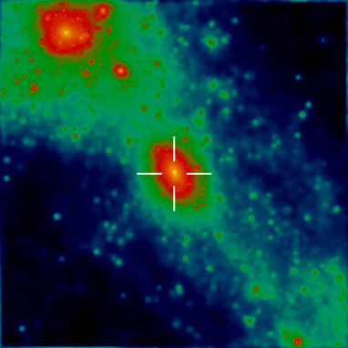
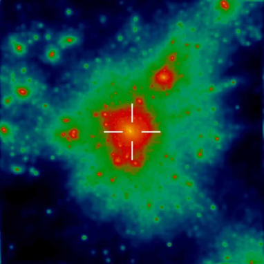
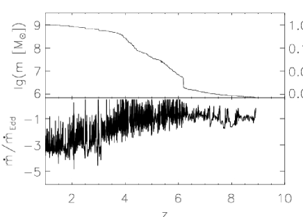
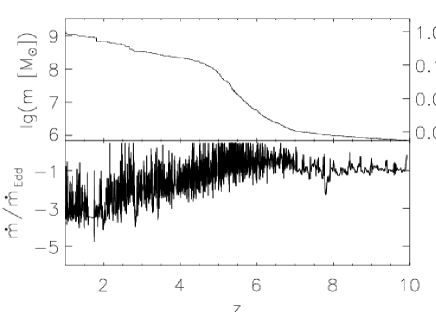
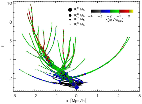
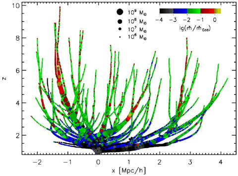
Figure 1: The $z=1$ environments of two high–mass BHs and their evolution. The images (top row) show the adaptively smoothed dark–matter density in volumes of size ($3.0\,h^{-1}$ Mpc)³. Each image is centered on the location of the black hole, which is also marked with cross hairs. In the middle row, the evolution of the black holes’ most massive progenitors’ masses with time, and the corresponding accretion rates, are shown. For the mass panels, we also show the fraction $f$ of the final mass. The two bottom panels show the merger trees, with redshift $z$ on the $y$–axis, and symbol sizes and colours depicting masses and accretion rates (see legend). The halo masses and the local densities are $1.44\cdot 10^{13}$ M_⊙ and $r_{13}=0.44\,h^{-1}$ Mpc (left column), and $4.07\cdot 10^{13}$ M_⊙ and $r_{13}=0.26\,h^{-1}$ Mpc (right column).

2 The Simulation

In this Section, we present a brief description of the simulation code and the simulation used in this work. We refer to Di Matteo et al. (2007) for detailed description of our method.

2.1 Methodology

2.1.1 Numerical Code

We use the massively parallel cosmological TreePM–SPH code GADGET2 (Springel 2005), with the addition of a multi–phase modelling of the ISM, which allows treatment of star formation (Springel & Hernquist 2003), and black hole accretion and associated feedback processes (Springel et al. 2005). The GADGET2 implementation of smoothed particle hydrodynamics (SPH; Monaghan 1992) uses a formulation which conserves energy and entropy despite the use of fully adaptive SPH smoothing lengths (Springel & Hernquist 2002). Radiative cooling and heating process (Katz et al. 1996) and photoheating due to an imposed ionizing UV background are included. To model star formation the multiphase model for star-forming gas developed by Springel & Hernquist (2003) is used. It has two principal ingredients, a star formation prescription and an effective equation of state. For the former, we a adopt a rate motivated by observations and given by the Schmidt–Kennicutt Law (Kennicutt 1989), where the star formation rate is proportional to the density of cold clouds divided by the local dynamical time, and it is normalized to reproduce the star formation rates observed in isolated spiral galaxies (Kennicutt 1989, Kennicutt 1998). The latter includes the self–regulated nature of star formation due to supernovae feedback in a simple model for a multiphase ISM.

2.1.2 Accretion and Feedback from Supermassive Black Holes

Analogous to the treatment of star formation and supernova feedback, a sub–resolution model for the accretion of matter onto a black hole and for the associated feedback is adopted. Full details of the model can be found in Di Matteo et al. (2005), Springel et al. (2005), and Di Matteo et al. (2007).

Black holes are represented by collisionless particles that grow in mass through accretion of gas from their environments. A fraction $\epsilon_{\rm f}$ of the energy released through radiation is put back into the system as it couples thermally to nearby gas to influence its motion and thermodynamic state. The underlying idea is that while the physics of the accretion disks around the black holes is not resolved, the large–scale feeding of galactic nuclei with gas, which is resolved, is the critical process that determines the growth of supermassive black holes.

BH collisionless ’sink’ particles are placed at the centers of galaxies. In the cosmological simulation discussed here, a friends–of–friends group finder (e.g.; Davis et al. 1985), called at regular intervals (the time intervals are equally spaced in log $a$, with $\Delta\log{a}=\log{1.25}$), is employed to find groups of particles. Each group that does not already contain a black hole is provided with one by turning its densest particles into a sink particle with a seed black hole mass of $10^{5}h^{-1}$ M_⊙. The black hole particle then grows in mass through either the accretion of gas or through mergers with other black hole particles. Note that the black hole seed mass is negligible compared to the accreted mass. For black holes with $z=1$ masses of $M_{\rm BH}=10^{7}$ M_⊙, on which the bulk of the following analysis is based, the seed mass contributes around 1% of the final mass or less. For a more detailed discussion of the motivation behind the choice of seed mass see Di Matteo et al. (2007).

The accretion onto the black hole from the large–scale gas distribution is modeled using a Bondi–Hoyle–Lyttleton parameterization (Hoyle & Lyttleton 1939, Bondi & Hoyle 1944, Bondi 1952), which relates the accretion rate onto the black hole, $\dot{M}_{\rm B}$, to the density $\rho$ and sound speed $c_{s}$ of the surrounding gas. For the simulation used in this work, it was assumed that accretion is limited to three times the Eddington rate, $\dot{M}_{\rm Edd}$. The radiated luminosity, $L_{\rm r}$, is related to the accretion rate, $\dot{M}_{\rm BH}$, through the radiative efficiency $\eta=L_{\rm r}/(\dot{M}_{\rm BH}\,c^{2})\,,$ which gives the amount of energy that can be extracted from the innermost stable orbit of the accretion disk. Here, a value of $\epsilon_{\rm r}=0.1$ was used, the mean value for a radiatively efficient accretion disk (Shakura & Sunyaev 1973) onto a non-rapidly rotating black hole. The model assumes that a fraction $\epsilon_{\rm f}=0.5$ of the released radiation couples to the surrounding gas in the form of feedback energy. For reasons of simplicity, this process is modeled as thermal energy deposited isotropically in the region around the black hole. In Di Matteo et al. (2005), $\epsilon_{\rm f}$ was fixed by fitting the $z=0$ $m_{\rm BH}-\sigma$ relation, and the value of $\epsilon_{\rm f}=0.5$ found there was also adopted in this work. This is the only parameter for the BH model, and our cosmological simulations have all parameters fixed from our previous work. Note that even though we do not run the cosmological simulation to $z=0$, we do use a value for $\epsilon_{\rm f}$ determined to match the $z=0$ $m_{\rm BH}-\sigma$ relation. A more detailed discussion of the motivation behind these choices plus a discussion of the predictions for the $m_{\rm BH}-\sigma$ relation at various redshifts (incl. comparisons with the available observational constraints) can be found in Di Matteo et al. (2008).

2.1.3 Mergers of Supermassive Black Holes

When galaxies merge their central black holes are also expected to merge at some stage. Thus, mergers generated through the hierarchical buildup of haloes and galaxies contribute to the growth of the central black holes. Some of the details of this process are still a matter of debate. Given the resolution of the simulations it is impossible to treat this problem in detail. Instead, it is assumed that two black hole particles merge if they come within the spatial resolution of the simulation and if their relative speed lies below the gas sound speed. Note that we also cannot resolve (nor accurately model) the ejection of black holes by gravitational recoil (see, for example, Hoffman & Loeb 2006), or by three–body sling–shot ejection of black holes in triple systems (see, for example, Baker et al. 2006).

2.2 Details of the Simulation

We use the standard $\Lambda$CDM cosmological model, with parameters chosen to match the first year Wilkinson Microwave Anisotropy Probe measurements (Spergel et al. 2003). The parameters are $\Omega_{0}=0.3$, $\Omega_{\Lambda}=0.7$, Hubble constant $h=0.7$, expressed in units of $H_{0}=100\,h$ km sec^-1 Mpc^-1, a scale–invariant primordial power spectrum with index $n=1$, and a normalization of the amplitude of fluctuations of $\sigma_{8}=0.9$. The more recent (third year) WMAP results, with their considerably lower value of $\sigma_{8}$, were published after the simulation had progressed quite far already (see however Evrard et al. 2007). For a discussion of the repercussions of the larger value of $\sigma_{8}$ on our cosmological simulations with black holes see also Sijacki et al. (2007).

The simulation is of a periodic box of size 33.75 $h^{-1}$ Mpc, using $486^{3}$ gas and dark–matter particles each. The size of the volume was motivated by the goal to achieve the highest possible resolution, while, at the same time, matching the suite of simulations in Springel & Hernquist (2003), to allow detailed comparisons between the physical properties of simulations with and without black holes. In addition, the box size and particle number were chosen such that the physical resolution at $z\sim 6$ is comparable to that of some of the previous work of galaxy mergers runs with black holes (see Di Matteo et al. 2005, Springel et al. 2005, Robertson et al. 2006). Following Di Matteo et al. (2007) we hereafter refer to this simulation as the BHCosmo run. Di Matteo et al. (2007) contains a very detailed discussion of, for example, the $m_{\rm BH}$–$\sigma$ and $m_{\rm BH}$–$m_{\rm Bulge}$ relations from the simulation, and we thus refer the reader interested in the details – which provide ample justification for the choices in the simulation methodology – to that work.

From a starting redshift of $z=157$, the simulation was evolved to a final redshift of $z=1$. A total set of 36 outputs was saved. In addition, whenever a black hole particle was accreting matter, its mass, accretion rate, and position was stored, as was information about which black hole merged with what other black hole at what redshift. For the 3,547 black holes that are contained in the simulation volume at $z=1$, a total of more than four and a half million progenitor black holes exists. From this raw data, the merger trees of all $z=1$ black holes were generated, with the most massive black hole counting more than one hundred twenty thousand progenitor black holes.

In addition to the BHCosmo box, there is a second simulation with the same cosmological parameters but a larger volume (its box size is 50.0 $h^{-1}$ Mpc), called E6, which, however, was only evolved until $z=3.82$ due to constraints on the available computing time. We will make use of E6 only for comparisons with BHCosmo at $z=5$, one of the times that will be studied in the following.

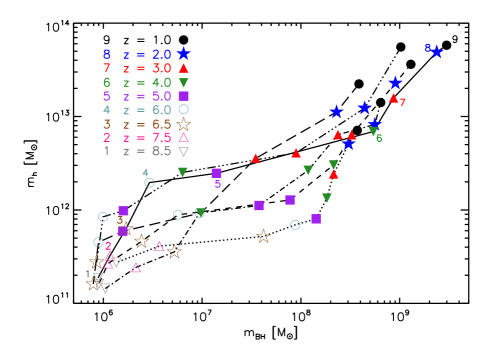
Figure 2: Black hole mass $m_{\mbox{\scriptsize{BH}}}$ versus host halo mass $m_{\mbox{\scriptsize{h}}}$ for six high–mass black holes, at nine different redshifts. We use different colours and symbols for the different redshifts, as shown in the legend. In addition, for one example, the numbers near the circles show how the graph has to be read. The most massive high–redshift black hole (dotted line) clearly stands out: It is more than one order of magnitude more massive at $z=6.5$ than the other black holes. And unlike all the other black holes, it only gains one order of magnitude in mass until the final redshift in the plot.

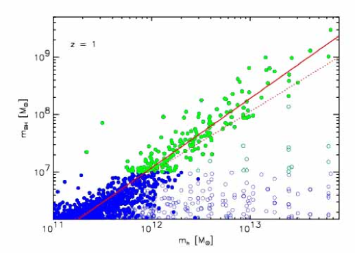
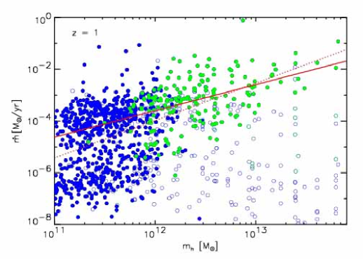
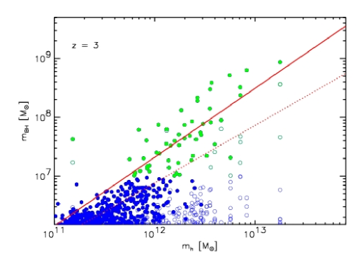
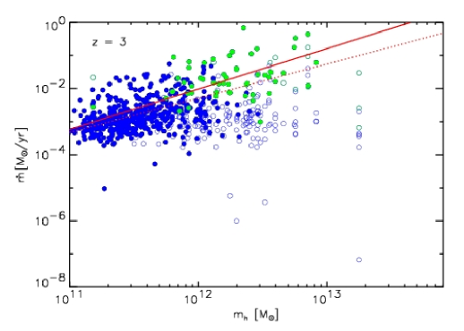
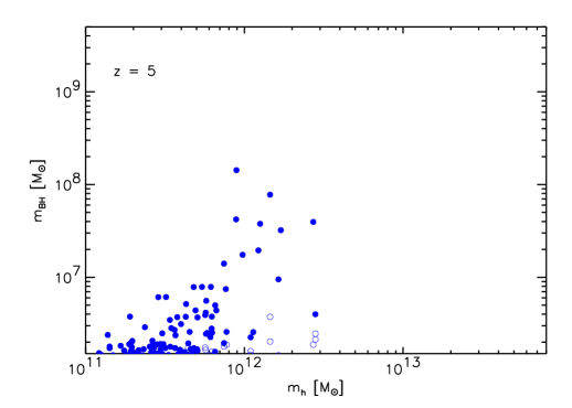
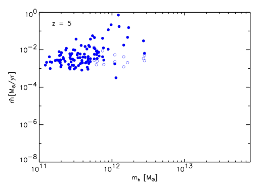
Figure 3: Left panels: Black hole mass $m_{\mbox{\scriptsize{BH}}}$ versus host halo mass $m_{\mbox{\scriptsize{h}}}$, with green (blue) symbols for BHs above (below) $1.0\cdot\,10^{7}$ M_⊙. Solid and open circles show main and satellite black holes, respectively. The solid (dotted) red line shows the best (linear) fit for the relation between $m_{\mbox{\scriptsize{BH}}}$ and $m_{\mbox{\scriptsize{h}}}$ for BHs more massive than $10^{7}\,\mbox{M}_{\odot}$ (for the full sample). Right panels: Black hole accretion rate $\dot{m}$ versus host halo mass $m_{\mbox{\scriptsize{h}}}$, using the same convention as in the left panels. The solid (dotted) red line shows the best (linear) fit for the relation between $\dot{m}$ and $m_{\mbox{\scriptsize{h}}}$ for BHs more massive than $10^{7}\,\mbox{M}_{\odot}$ (for the full sample). From top to bottom, data at redshifts $z=1$, $z=3$, and $z=5$ are shown. Because of the paucity of data points at $z=5$, we do not attempt to fit those data.

3 The BH–Halo Connection

3.1 The Co–Evolution of BHs and Their Host Haloes and the Anti–hierarchical formation of the most massive BHs

The most immediate environment of a black hole is its host galaxy and, by extension, its host halo. The formation of a dark matter halo, unlike that of a galaxy, is solely governed by gravity. Haloes grow through the accretion of matter and through mergers. Both processes also contribute to the growth of the baryonic component of galaxies, as gas is added, some of which then forms new stars. But unlike in the case of the dark matter, the growth of the baryonic component and of BHs depends on complex hydrodynamical processes, including gas cooling, mergers, feedback due to supernovae and AGNs which may expel some of the gas from the galaxies’ potentials. The interplay between these processes and their relative importance are subject to numerous studies such as, for example, those involving semi–analytical models of galaxy formation (for a detailed review of such models, and many references, see Baugh 2006). Di Matteo et al. (2007) already contains detailed descriptions of the relationship between the properties of BHs and of the subhaloes or galaxies they reside in, through a study of the evolution of the $m_{\rm BH}-\sigma$ and $m_{\rm BH}-m_{*}$ relations. For a discussion of those relationships we refer to that work. Unless noted otherwise, in the following we will present results from the BHCosmo simulation.

In the top panels of Figure 1, we show two examples of the dark matter distribution in the immediate surrounding of two of the most massive black holes at $z=1$. The BH and halo mass on the left (right) are $9.89\cdot 10^{8}$ M_⊙ and $1.44\cdot 10^{13}$M_⊙ ($1.30\cdot 10^{9}$ M_⊙ and $4.1\cdot 10^{13}$ M_⊙), respectively. The locations of the black holes within their host halos are marked with cross hairs. Each picture shows the adaptively smoothed dark–matter density in volumes of size ($3.0\,h^{-1}$ Mpc)³.

In the middle row of Figure 1, we illustrate the mass assembly histories of the black holes shown in the top panels. We plot the instantaneous BH mass and the fraction of the final BH mass, and accretion rate (in units of Eddington) as a function of redshift. It is evident that these objects experienced major critical accretion phase (and hence BH mass growth) epochs at high redshifts, in the range of $4<z<7$. For $z<4$, the BH accretion rates decrease, showing far more sporadic episodes of critical Eddington growth and a drop of the average accretion rates of about two orders of magnitude for $z\simeq 2$ and later. A BH mass of $\sim 4-5\cdot 10^{8}$ is assembled by $z\sim 4$, which roughly doubles by $z\sim 1$.

Lastly, in the bottom row of Figure 1 we show the merger trees of the two black holes. Redshift is given on the $y$–axis; the $x$–axis is one of the actual coordinates (both black holes are set to be at the coordinate origin at $z=1$). Symbol sizes and colours are scaled to reflect masses and accretion rates, respectively, with each decade in accretion rate using a different colour. Just like in the cases discussed in Di Matteo et al. (2007), the histories of these massive black holes are quite complex. Even though the two black holes have comparable masses as a result of a roughly similar accretion history, the BH shown in the right column experiences many more merger events than the one in the left column. Since the two black holes appear to be residing in somewhat different large–scale environments, this indicates that the properties of the BHs can be affected by the large–scale matter configuration. We will investigate the influence of large–scale environment on black hole properties in Section 4.

It is instructive to compare Figure 1 with Figures 4 and 5 in Malbon et al. (2007), who use a semi–analytical galaxy formation model to study the growth of supermassive black holes (note the difference in the BH masses). While here we only trace the evolution of the BHs, our direct simulation provides us with an amount of detail unmatched by the semi–analytical ansatz, since our simulation method stores information about the black holes whenever the are active or merging (resulting in many thousands of different periods of activity for the most massive of our BHs). In contrast, semi–analytical galaxy formation models are restricted to constructing the histories of BHs on top of merger trees of dark matter haloes which are typically a lot sparser (fifty or one hundred output times).

Figure 1 indicates noticeable differences in the growth histories of these massive black holes. To further characterize the evolution of haloes and their black holes, Figure 2 shows the growth history of BH mass, $m_{\mbox{\scriptsize{BH}}}$, and host halo mass, $m_{\mbox{\scriptsize{h}}}$, for a sample of six high–mass ($m_{\mbox{\scriptsize{BH}}}\geq 10^{8}$ M_⊙) black holes. Shown are BH and respective host halo mass at nine different redshifts, starting from $z=8.5$ and ending at $z=1.0$. The growth curves in Figure 2 show the histories of the same sample of massive black holes discussed in Di Matteo et al. (2007; see their Figure 13). The figure shows that at first the black holes’ masses grow relatively slowly compared with their host halo masses (for $z>7$), followed by rather rapid growth between redshifts of $z\simeq 6$ and $z\simeq 3$. During this time most black holes in this sample have increased their masses by two orders of magnitude while their host haloes’ masses increase by most an order of magnitude. This is depicted by the rather flat region in the curves in Figure 2 at redshifts $6<z<3$. The curves steepen again at $z<3$ as the growth of the parent halo offsets that of its BH. The dashed line shows the black hole and halo in the right column of Figure 1. As is clear from this Figure, the growth of haloes and black holes is quite different from each other. As discussed earlier, BH gas accretion in these high mass systems is the highest at $z>4$, leading to the build–up of the bulk of the BH mass, which is later supplemented by a large number of merger events at lower redshifts. Note that, as discussed in Di Matteo et al. (2007), the most massive black hole in the simulation at $z=6.5$ is more than an order of magnitude more massive at than any of the other black holes. Its black–hole–to–halo mass ratio is also the largest all the way to $z\sim 4$ (as shown by the dotted line in Fig. 2). However, below this redshift the BH only gains one order of magnitude in mass and is overtaken by most of the other objects.

In a $\Lambda$CDM cosmology, dark matter haloes – such as those in Figure 2 – form hierarchically. Small haloes assemble first, and through mergers and accretion, larger and larger haloes are built. Maulbetsch et al. (2007) provide an instructive study of the mass assembly histories of dark matter haloes in a very large simulation volume, which here, and in the following sections, can be used to compare black hole assembly histories with dark matter assembly histories. The complex relationship between halo and BH masses in Figure 2 indicates that the massive black holes in those haloes do not follow this pattern. Instead, high–mass black holes are assembled early compared to their host halos. We will further discuss this ’anti–hierarchical’ behaviour in Section 3.3.

3.2 BH Host Halo Masses

After studying the co-evolution of the most massive black holes and their host haloes, we now broaden the investigation and look at the demographics of black holes of all masses in their dark matter haloes. In the left panels of Figure 3 we show the relation between host halo mass, $m_{\mbox{\scriptsize{h}}}$, and BH mass, $m_{\mbox{\scriptsize{BH}}}$, at redshifts $z=1$, $z=3$, and $z=5$ (from top to bottom) with green (blue) symbols for BHs above (below) $1.0\cdot\,10^{7}$ M_⊙. We show main (or central) BHs with solid circles and satellite BHs with open circles. For each halo, the main black hole is considered to be the one that resides at the center of the most massive subhalo. Satellite BHs are those that reside at the center of galaxies that orbit around the central, typically most massive galaxy (see, e.g., Fig. 7 in Di Matteo et al. 2007). Note that the smallest haloes that contain a BH in the simulation always consist of two thousand or more particles in the BHCosmo run and are therefore very well resolved.

Following Ferrarese (2002), we determine the relation between $m_{\mbox{\scriptsize{BH}}}$ and $m_{\mbox{\scriptsize{h}}}$ in

$$\frac{m_{\mbox{\scriptsize{BH}}}}{10^{8}\,\mbox{M}_{\odot}}=c(z)\left(\frac{m_{\mbox{\scriptsize{h}}}}{10^{12}\,\mbox{M}_{\odot}}\right)^{\alpha}$$ (1)

We let the fit cover black holes with masses larger than $10^{7}\,\mbox{M}_{\odot}$ (the range for which large numbers of observational data are available) and all black holes. We allow for $\alpha$ and $c$ to be redshift dependent. For the $m_{\rm BH}\geq 10^{7}\,\mbox{M}_{\odot}$ sample and redshifts $z=1$, $z=3$ we find $\alpha=1.21\pm 0.05$, $\alpha=1.17\pm 0.14$, and $c=0.12\pm 0.01$, $c=0.21\pm 0.03$, respectively. The full sample yields $\alpha=1.05\pm 0.02$, $\alpha=0.98\pm 0.04$, and $c=0.10\pm 0.01$, $c=0.08\pm 0.02$ for the redshifts $z=1$, $z=3$, respectively. In the left panels of Figure 3 we show the fits superimposed as a solid (dotted) red line for the $m_{\rm BH}\geq 10^{7}\,\mbox{M}_{\odot}$ (full) sample. Because of the small number of objects at $z=5$ and their large scatter, we do not attempt a fit.

Observationally, the $m_{\mbox{\scriptsize{BH}}}-m_{\mbox{\scriptsize{h}}}$ relation (eq. 1) can only be determined indirectly, since the masses of the dark matter haloes cannot be measured directly. For example, Ferrarese (2002) uses an $m_{\mbox{\scriptsize{h}}}-v_{\scriptsize{vir}}$ relation (where $v_{\scriptsize{vir}}$ is the halo velocity at its virial radius) from numerical simulations and then connects the haloes’ $v_{\scriptsize{vir}}$ with the circular velocities, $v_{c}$, of the BH host galaxies, using models for halo profiles. That way, the black hole masses can be related to the masses of their host haloes. For a local set of BHs, Ferrarese (2002) finds $\alpha=1.82$ and $c=0.03$, $\alpha=1.65$ and $c=0.1$, and $\alpha=1.82$ and $c=0.67$ for an isothermal dark matter profile, an NFW profile (Navarro et al. 1997), and a profile based on weak lensing results by Seljak (2002), respectively. An example of a more recent result is provided by Shankar & Mathur (2007) who find $\alpha=1.39$ and $c=(58/700)(1+z)$, or $c=0.17$, $c=0.33$, and $c=0.50$ for $z=1$, $z=3$, and $z=5$, respectively.

Finally, in the right panels of Figure 3 we show the relation between host halo mass, $m_{\mbox{\scriptsize{h}}}$, and BH accretion rate, $\dot{m}$ (in M_⊙/year), at redshifts $z=1$, $z=3$, and $z=5$ (from top to bottom). Just like in the panels on the left–hand side, satellite BHs constitute a distinguishable population, predominantly at lower accretion rates than the main BHs in the same halo. In the same fashion as for the black hole masses, we determine the relation between $\dot{m}$ and $m_{\mbox{\scriptsize{h}}}$ in

$$\dot{m}=d\,m_{\mbox{\scriptsize{h}}}^{\beta}$$ (2)

For the $m_{\rm BH}\geq 10^{7}\,\mbox{M}_{\odot}$ sample and redshifts $z=1$ and $z=3$ we find $\beta=1.01\pm 0.18$ and $\beta=1.22\pm 0.37$, respectively. The full sample yields $\beta=1.45\pm 0.08$ and $\beta=1.04\pm 0.06$ for the redshifts $z=1$ and $z=3$, respectively. The slopes are quite similar to those found for the $m_{\mbox{\scriptsize{BH}}}-m_{\mbox{\scriptsize{h}}}$ relation above, albeit with larger scatter. However, when we divide the sample using accretion rate instead of black hole mass a different picture emerges. Using only the most active black holes (with $\dot{m}\geq 10^{-2}$ M_⊙/year), at $z=1$, $\beta=-0.02\pm 0.14$, whereas at $z=3$, $\beta=0.66\pm 0.12$. That is, at $z=1$, there is virtually no relation between BH accretion rates and their halo masses, and at $z=3$, there is a very slight dependence. This result is fully consistent with the lack of a luminosity dependence in the clustering of AGNs in the DEEP2 sample as measured by Coil et al. (2007).

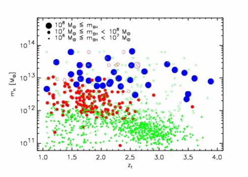
Figure 4: Formation redshift $z_{f}$ versus host halo mass $m_{h}$ for all black holes. The symbol sizes (and colours) depict different masses (see legend). In addition, filled and empty circles show central and satellite BH, respectively.

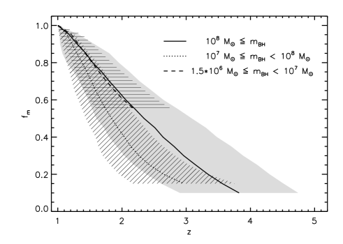
Figure 5: Mean assembly redshifts $z$ at which fractions $f_{m}$ of the largest progenitor masses were assembled for the mass ranges $1.5\cdot 10^{6}$ M${}_{\odot}\leq m_{\mbox{\scriptsize{BH}}}<10^{7}$ M_⊙ (dashed/green), $10^{7}$ M${}_{\odot}\leq m_{\mbox{\scriptsize{BH}}}<10^{8}$ M_⊙ (dotted/red), and $m_{\mbox{\scriptsize{BH}}}\leq 10^{8}$ M_⊙ (solid/blue). See main text for more details.

3.3 Formation Epochs

As already outlined in Section 3.1, the evolution of the most massive black holes does not mirror that of their host haloes. Is the same true for all black holes? For this and the following Sections, we divide the black–hole sample into three mass ranges, which we will refer to as the low, intermediate, and high–mass sample. The masses covered in these samples are $10^{6}$ M${}_{\odot}\leq m_{\rm BH}<10^{7}$ M_⊙, $10^{7}$ M${}_{\odot}\leq m_{\rm BH}<10^{8}$ M_⊙, and $10^{8}$ M${}_{\odot}\leq m_{\rm BH}$, respectively.

Figure 4 shows the formation redshift $z_{f}$ versus host halo mass $m_{h}$ for all black holes. Here, $z_{f}$ is defined as the redshift at which a black hole’s most massive progenitor for the first time contained half of its $z=1$ mass. Different symbol sizes (and colours) give the three different mass bins as indicated in the legend. As in previous Figures, filled and open circles indicate main and satellite BHs, respectively.

As expected in the standard hierarchical scenario, a large number of small black hole systems forms first, and these BHs are followed by intermediate and high mass systems at lower redshifts. However, Figure 4 also confirms our earlier finding (Section 3.1), namely that a large fraction of the high mass black holes have formation redshifts $z>2.5$. The formation redshifts of the largest BHs cover the full range of $z_{f}$. Thus, while very massive haloes form last in a hierarchical structure formation scenario, massive black holes are decoupled from this process.

Figure 5 relaxes the condition that the formation redshift is the redshift at which half the $z=1$ was first assembled in the largest progenitor. Instead, here the fraction $f_{\rm m}$ of final mass is now given on the y–axis, and the redshift at which that mass fraction was first assembled can be read of from the x–axis (the $f_{\rm m}=0.5$ case corresponds to our earlier definition of formation redshift). The shaded and dashed areas around the mean are the rms around that mean. Regardless of the mass fraction used to define $z_{f}$, the most massive black holes always have the highest average formation redshifts (note that because of the choice of seed black hole mass in the simulation, for the lowest mass black holes in Figure 5, a formation redshift can only be determined down to $f_{\rm m}=0.5$). This clear antihierachical assembly of BH mass in our simulation is consistent with the presence of high–$z$ quasars and thus provides a promising result of the self–consistent modelling of black hole growth in our cosmological simulations.

A comparison with Malbon et al.’s (2007) semi–analytical results is instructive, even though it is extremely important to remember the differences in the final redshifts (unlike in our case, Malbon et al. evolved their model until $z=0$). Their Figure 11 (right–hand column) can be compared with Figures 4 and 5. At $z=0$, these authors find hierarchical assembly of BH mass (using 50 or 95 percent of the final BH mass). Our results albeit at $z=1$, see hierarchical assembly for all but the most massive black holes. Given the formation histories of dark matter haloes, where the most massive haloes merge at redshifts below $z=1$, our results do not appear to contradict Malbon et al.’s: One can expect the massive BHs in very massive haloes to merge at $z<1$, thus shifting the formation redshifts of $z=0$ to the values seen in Malbon et al. It is interesting to note also that the BH formation redshifts are also very similar to the formation redshifts of the brightest cluster galaxies (BCGs) in De Lucia & Blaizot (2007).

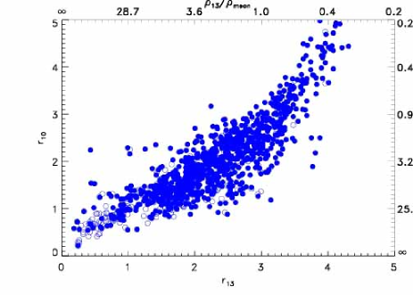
Figure 6: Adaptive density measures $r_{13}$ versus $r_{10}$ for all black holes in the sample.

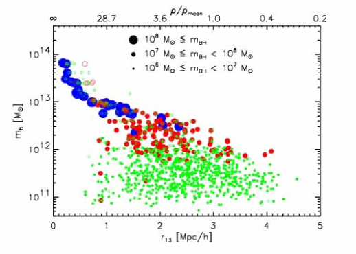
Figure 7: $z=1$ BH local density $r_{13}$ versus host halo mass $m_{h}$, using different size symbols (and colours) for three different mass ranges. In addition, we use closed and open circles for main and satellite BHs.

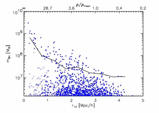
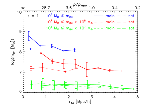
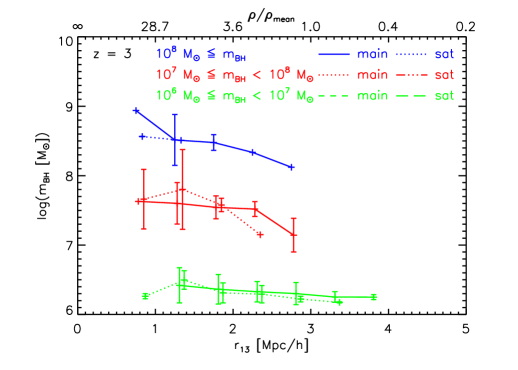
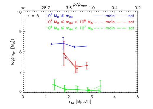
Figure 8: Upper left panel: $z=1$ BH local density $r_{13}$ versus black hole mass $m_{\rm BH}$, using closed and open circles for main and satellite BHs, respectively. Superimposed as a solid line is the mean for all BHs with $M_{\rm BH}\geq$10${}^{7}\,$M_⊙. Upper right and bottom panels: Distributions of the median values for three different redshifts, using different size symbols (and colours) for three different mass ranges and with error bars showing a 25% spread.

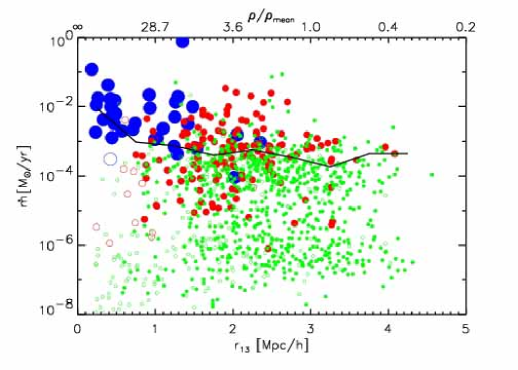
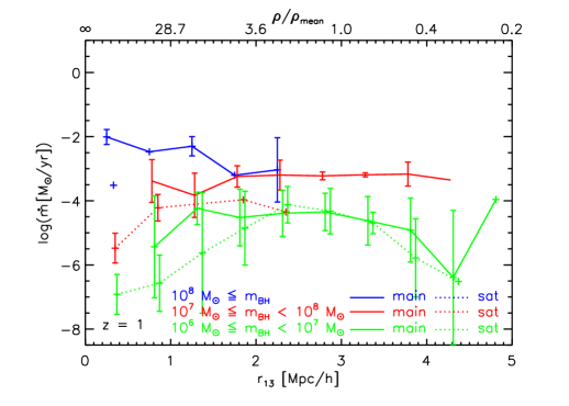
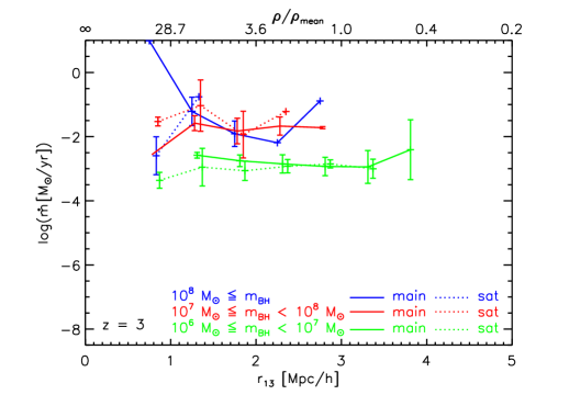
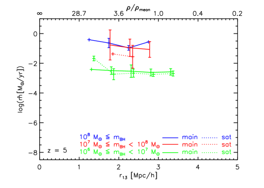
Figure 9: Upper left panel: $z=1$ BH accretion rate as a function of the local density $r_{13}$, using different size symbols (and colours) for three different mass ranges. In addition, we use closed and open circles for main and satellite BHs. Superimposed as a solid line is the mean for all BHs with $M_{\rm BH}\geq$10${}^{7}\,$M_⊙. Upper right and bottom panels: Distributions of the median values for three different redshifts, using the same colours for the BH mass ranges as in the upper left panel and with error bars showing a 25% spread.

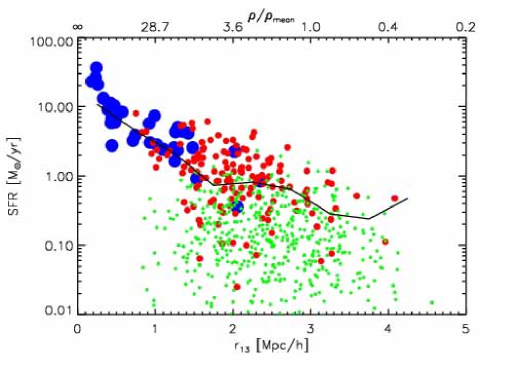
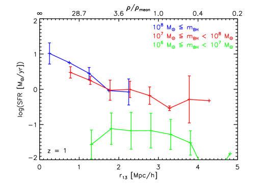
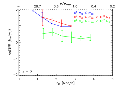
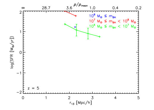
Figure 10: Upper left panel: $z=1$ star formation rates in galaxies that host BHs as a function of the local density $r_{13}$, using different size symbols (and colours) for three different mass ranges. Superimposed as a solid line is the mean for all BHs with $M_{\rm BH}\geq$10${}^{7}\,$M_⊙. Upper right and bottom panels: Distributions of the median values for three different redshifts, using the same colours for the BH mass ranges as in the upper left panel and with error bars showing a 25% spread.

4 BHs and Their Environments

4.1 The Large–Scale Environments of BHs

Having explored the connection between black holes and their host haloes, we now look at the influence of the large–scale environment on the growth of supermassive black holes. Images of slices through our simulation volume (see Di Matteo et al. 2007) show a plethora of environments, ranging from small clusters/groups to voids and filaments. Our goal is to define a measure of density that preserves these different environments and that makes use of the fact that because of the large number of particles in our simulation volume we sample the underlying density field extremely well. Inspired by the SPH treatment, where the local density around a particle is determined by the distance to its $n$th neighbour (with $n$ typically of the order of 32 or 64), we quantify the large–scale environment through the quantity $r_{13}$, which for each black hole gives the radius of the sphere centered on that black hole that contains a mass of $10^{13}$ M_⊙. Mean density corresponds to about $r_{13}\approx 3.0\,h^{-1}$ Mpc. This is an adaptive density measure, which has the advantage of not blurring clusters or filaments into the voids (both theoretical and observational studies of voids have shown that their edges are rather steep; see Benson et al. 2003 or Colberg et al. 2005 for examples). A drawback of using $r_{13}$ is that it cannot be easily interpreted in a linear–theory framework.

Adaptive measurements of local environment, such as the one adopted here, are recently becoming increasingly common in observational studies, too – essentially, for the same reasons that we just outlined. For example, for volume–limited samples drawn from the SDSS, Park et al. (2007) define environment via a Spline kernel containing 20 $L_{*}$ galaxies. And Cooper et al. (2005) finds that the projected $n$–th nearest neighbour distance is the most accurate estimate of galaxy density for the DEEP2 galaxy samples. To show that $r_{13}$ is in fact quite similar to measuring the distance to an $n$–th neighbour, in Figure 6, we show the relationship between $r_{13}$ and $r_{10}$, where for each black hole $r_{10}$ is the distance to the 10th–nearest neighbour (solid and open circles show main and satellite BHS, respectively). As can be seen $r_{13}$ and $r_{10}$ are pretty well correlated and hence provide consistent measure of local enviroment. Here we adopt $r_{13}$ as that makes use of the full density field in the simulations.

In Figure 7, we show how black holes populate their host haloes and environments at $z=1$. Each black hole is represented by a circle (as before open and closed for satellite and main BHs, respectively), and plotted in the $m_{\rm h}$–$r_{13}$ ($\rho/\rho_{\rm mean}$) plane. The most massive haloes, which reside in the highest density regions, contain the most massive black holes. These populate the regions of $\rho/\rho_{mean}>$ a few, i.e. what we would identify as cluster/group like environments and filaments. Regions of low density (with $r_{13}>3\,h^{-1}$ Mpc or, equivalently, $\rho/\rho_{mean}<1.0$) contain only haloes with masses lower than $10^{12}$ M_⊙ and BHs with masses lower than $10^{7}$ M_⊙. It is interesting to note that black holes with masses in the range $10^{7}\hbox{$\rm\thinspace M_{\odot}$}\geq M_{\rm BH}\leq 10^{8}\hbox{$\rm\thinspace M_{\odot}$}$ can be found across the whole range of densities (see also Section 4.3). Also note that satellite black holes populate the full range of densities.

While Figure 7 contains information about the BHs as a function of host halo mass and large–scale environment, in the following we will restrict our focus to large–scale environment only, as we have already discussed the explicit one–to–one relation of $m_{\rm BH}$ versus $m_{\rm h}$ in Figure 2. The upper left panel in Figure 8 shows black hole masses $m_{\rm BH}$ as a function of local density, $r_{13}\;(\rho/\rho_{\rm mean})$ and the mean for all black holes with $M_{\rm BH}\geq$10${}^{7}\,$M_⊙. Overall, there is a rough mean dependency with $m_{\rm BH}\sim(\rho/\rho_{\rm mean})^{-3/2}$ for black holes with $M_{\rm BH}\geq$10${}^{7}\,$M_⊙. As noted above, larger mass BHs live in denser environments, while intermediate to low mass BHs reside across a large range of densities.

In the three additional panels in Figure 8 we show the median $m_{\rm BH}$ as a function of $r_{13}$ for the three mass bins introduced before at three different redshifts $z=1$ (upper right panel), $z=3$ (lower left panel), and $z=5$. For $z=5$, we take black holes from the E6 simulation, which – due to its larger volume – contains more objects. As before, we also divide the BH samples into main (solid lines) and satellite (dotted lines) BHs, and the error bars show the 25% percentiles around the median. At both $z=1$ and $z=3$ the density dependence decreases across BH mass bins, with the highest BH mass bin (blue symbols) showing the strongest dependence and the lowest BH mass bin (green symbols) having none. Also note that the three panels reflect the overall growth of structure between $z=5$ and $z=1$: as cosmic time progresses, an increasingly larger range of densities gets covered.

Using the same panel structure as in Figure 8, Figure 9 shows the density dependency of black hole accretion rates, again with E6 data used for $z=5$. $\dot{m}$ spans a much larger dynamic range than $m_{\rm BH}$. However, its overall mean density dependence is similar to that of $M_{\rm BH}$. We find that approximately $\dot{m}\propto(\rho/\rho_{\rm mean})^{-3/2}$ for $M_{BH}\geq 10^{7}\hbox{$\rm\thinspace M_{\odot}$}$, albeit with much larger scatter across all densities. In addition, at $z=1$, the most active black holes (with $\dot{m}\geq 1.0\cdot 10^{-2}$ M_⊙/year) avoid underdense regions, that is they can be found in environments with $r_{13}<3.0\,h^{-1}$ Mpc (or $\rho/\rho_{\rm mean}>1.0$). Enhanced accretion in higher density regions is consistent with the overall picture that gas rich mergers (which are occuring in such regions) are the main trigger of quasar phase as also supported from the analysis in Di Matteo et al. (2007). Note that if we expressed the black hole accretion rates in Eddington units we would be washing out some of our result because of the additional BH mass dependence in Eddington rates.

At $z=1$, satellite black holes have lower accretion rates than central black holes. This is because their host haloes had their gas stripped when they fell into the large halo (Gunn & Gott 1972, see Moore et al. 2000 for a review). We find that the hosts of satellite black holes – themselves satellites inside their host halo – either have sharply reduced gas fractions or no gas left at all. The upper right and the two bottom panels (redshifts $z=1$, $z=3$, and $z=5$) show that black holes in each of the three mass samples have larger accretion rates at earlier times. What is more, the density dependence of the accretion rates of the most massive black holes is more pronounced at $z=3$ than at $z=1$. This result is also expected as gas fraction in galaxies and the mergers rates, responsible for the strong quasar evolution decline with decreasing redshift (see also Di Matteo et al. 2007).

Most of the discussion above concentrated on the sample of black holes with masses $M_{\rm BH}\geq 10^{7}\hbox{$\rm\thinspace M_{\odot}$}$. Resolution effects are a concern at the low–mass end of the black hole sample. While haloes in the mass range considered throughout this work are very well resolved – a halo of mass $10^{11}$ M_⊙ consists of almost three thousand particles – accretion onto the black holes with masses close to the seed mass are likely to be not so well resolved. For the black holes considered here, we require each BH to have at least twice the seed hole mass – in part so that we can reliably determine a formation redshift $z_{f}$. But this requirement does not necessarily prevent problems due to resolution effects. Some investigations we performed by splitting up the low BH mass bins in subsample did not show indications for resolution issues biasing our density dependence result. To test for this directly however, a higher resolution simulation would be needed.

We now compare the density dependence of black hole masses and accretion rates with that of the star–formation rates (SFRs) of their host galaxies (see also Croft et al. 2008). In Figure 10, we show SFRs in the BH host galaxies, using the same notations as in Figures 8 and 9. We first note that in Figure 10, satellite galaxies (galaxies that contain what we earlier called satellite BHs) are absent. With the exception of a handful of galaxies in the lowest BH mass range, which have very small SFRs, satellite galaxies in the simulation form no stars, a fact that – again – supports the picture of most of the gas being stripped from haloes/galaxies after they have fallen into a larger halo. There are, of course, two gas components, namely cold gas and hot gas. Simulations by McCarty et al. (2008) indicate that haloes might retain around 30% of their hot gas after falling into a larger halo. The hot gas would then have to cool, however, to be able to form stars – something which does not appear to be happening in our simulation (recall though that the simulation was only run until $z=1$, which severely limits the actual time available to cool gas). This picture is also supported by the simulations run by and analyzed by Kereš et al. (in preparation), where star formation in satellite haloes/galaxies is severely quenched after redshifts of $z\approx 3$ (Katz, private communication).

Figure 10 shows that at all redshifts, SFR is perhaps the strongest function of density, with SFR $\propto(\rho/\rho_{\rm mean})^{-2.0}$. SFRs are also highest in galaxies with the most massive central BHs and increase with increasing redshift. Although a detailed discussion of SFR in the simulation is beyond the scope of this work and will be done elsewhere we are interested in its relation to BH accretion. It is important, however, to point out that the dependence of SFR on density in the simulations is is completely consistent with the $z=1$ results reported by Elbaz et al. (2007), who find an increase in SFR with local density in the GOODS data (see their Figure 8), and by Cooper et al. (2007) using DEEP2 data. Note this trend is reversed at $z=0$, (see, for example, Kauffmann et al. 2004). Note that semi–analytical galaxy model in the Millennium Run (Croton et al. 2006) fail to reproduce this increase in SFR with density (Fig.’s 8 and 9 in Elbaz et al. 2007). This agreement of the dependence of SFR on local density at $z=1$ provides further support for the validity of the model used in our simulations and the reliability of the trends discussed here.

In particular, as it is already apparent from Figures 9 and 10, there is no one to one relationship between black hole accretion and star–formation rates of the host galaxies. While BH accretion does depend somewhat on environment, star formation rates show a stronger dependence. Such results are consistent with quasar enviroments corrresponding to group/small group scales, where major gas rich mergers will be most efficient, whereas the majority of the star formation simply occurs in regions of high density and high concentration, and most of it in a quiescent mode (see also Di Matteo et al. 2007). In Figure 11, we compare directly the BH accretion rates and the SFRs of their hosts directly. For fixed accretion (SFR), there is a wide range in SFR (accretion), for all black hole mass ranges considered here.

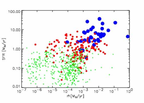
Figure 11: Accretion rate $\dot{m}$ versus SFR, both in M_⊙/yr for main BHs. As in the previous Figures, the symbol sizes and colours reflect the three BH samples discussed throughout this work.

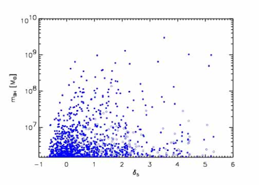
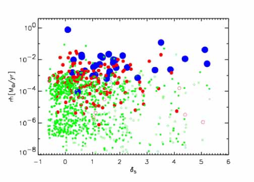
Figure 12: Left panel: $z=1$ BH overdensity $\delta_{5}$ versus mean BH mass $m_{\rm BH}$ (using the same style as in Figures 8 and 9) from the BHCosmo simulation. Right panel: The same for the mean accretion rate.

4.2 Environmental density estimates

As seen in Figures 8, expressing the environment through $r_{13}$ makes the most massive BHs lie predominantly in the densest regions, while the lowest density regions are occupied mostly by small BHs. As already indicated above, while observational studies have been increasingly using an adaptive measure of density, in the past, studies often determined the density around a position in space using spheres of fixed radius, typically a few Megaparsecs (with 8 $h^{-1}$ Mpc a particularly common choice). To what extent do our results depend on our choice of an adaptive measurement of density? To investigate this question, we here repeat some of our analysis by adopting a different measure of density. We define the quantity $\delta_{5}$, the overdensity in spheres of radius 5 $h^{-1}$ Mpc, around the position of a BH, which is equivalent to smoothing the mass distribution with a Top Hat kernel of size 5 $h^{-1}$ Mpc. The two panels in Figure 12 show plots equivalent to the upper left panels in Figures 8 and 9, but with $\delta_{5}$ replacing $r_{13}$. The relatively tight relationship between the densest region and the most massive BHs from Figure 8 disappears. This is not surprising and it is due to the fact that 5 $h^{-1}$ Mpc is much larger than the virial radius of one of the large haloes in the simulation, so $\delta_{5}$ is a probe of the mass inside and around these haloes. In other words, while $\delta_{5}$ contains information about a scale of 5 $h^{-1}$ Mpc, which is a typical scale for black holes sitting in a small group or filament like enviroment, it is way too large for black holes in larger groups/clusters. The right panel of Figure 12 shows most the density dependence from Figure 9 washed out, with virtually no dependence of the accretion rate on environment. As already mentioned, using $\delta_{5}$ amounts to smoothing the mass distribution with a filter of that size, thus erasing all information on smaller scales. We are thus led to conclude that there exist environmental trends for the black holes in our simulation volume, with the scales on which these trends can be found being below 5 $h^{-1}$ Mpc. In other words, the environmental differences found in our simulation volume exist on scales which are non–linear, a situation comparable to what is found observationally (see, for example, Kauffmann et al. 2004, Blanton & Berlind 2007, Park et al. 2007 – all for $z=0$). This is no surprise also because both star formation and black hole accretion depend strongly on local density enhancements.

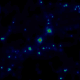
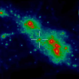
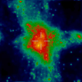
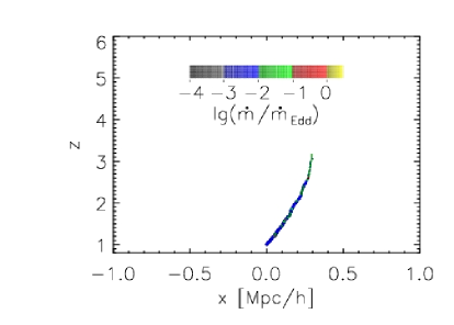
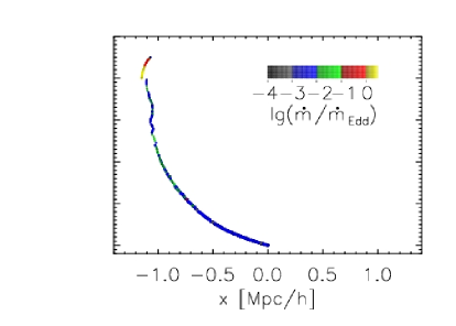
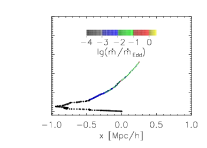
Figure 13: Three low–mass BH in regions of different density. From left to right, depicted are a low–density region, a high–density region, and a cluster. The halo masses and the local densities are $1.63\cdot 10^{11}$ M_⊙ and $r_{13}=4.0\,h^{-1}$ Mpc (left column), $2.8\cdot 10^{11}$ M_⊙ and $r_{13}=1.2\,h^{-1}$ Mpc (central column), and $6.25\cdot 10^{13}$ M_⊙ and $r_{13}=0.27\,h^{-1}$ Mpc (right column). The images show the adaptively smoothed dark–matter density in volumes of size ($3.0\,h^{-1}$ Mpc)³. Each image is centered on the location of the black hole, which is also marked with cross hairs.

4.3 Low–Mass BHs and their environments

In Figure 4, there exists an interesting population of black holes with formation redshifts higher than 2.5. This population contains only a small number of the intermediate–mass black holes and about half of the high–mass ones, but large numbers of black holes with masses lower than $10^{7}$ M_⊙. These latter BHs are composed of two populations, main BHs present in small (less massive than $\approx 10^{12}$ M_⊙) haloes and satellite BHs embedded in larger haloes.

The non–satellite low–mass BHs are an interesting population of objects, especially since they cover the full range of local densities but a fairly narrow range of host halo masses. For these black holes to have such low masses and high formation redshifts, they cannot have been accreting much gas (or experience many mergers). Such conditions are expected to exist in low–density regions such as voids, where the growth of haloes is truncated towards low–mass haloes, with very slow growth with redshift (Gottlöber et al. 2003). However, Croton et al. (2007) have shown that in the neighbourhoods of massive systems, and hence in high–density environments, most of the material is accreted onto those large haloes, leaving smaller haloes nearby to starve. We now investigate such stifled growth in the population of low–mass black holes.

To illustrate directly the variety of environments of the population of low–mass BHs in the simulation, in Figure 13 we show three black holes located in small haloes in a low–density region (left column), a high–density region (middle column), and inside a much larger halo (right column). The local densities and the halo masses for these black holes are $r_{13}=4.0\,h^{-1}$ Mpc, $r_{13}=1.2\,h^{-1}$ Mpc, and $r_{13}=0.27\,h^{-1}$ Mpc and $m_{\rm h}=1.63\cdot 10^{11}$ M_⊙, $m_{\rm h}=2.8\cdot 10^{11}$ M_⊙, and $m_{\rm h}=6.25\cdot 10^{13}$ M_⊙ for the left, middle, and right columns, respectively. We have focused on the extreme ends of $r_{13}$, picking objects with roughly the same mass. In each column, the top panel shows the location of the black holes in the adaptively smoothed dark–matter distribution in a volume of size ($3.0\,h^{-1}$ Mpc)³, with the panel centered on the black hole (the locations of the black holes are also marked with cross hairs). The central panel shows the mass growth (top parts) and accretion histories (bottom parts) of these black holes. Just like in Figure 1, the bottom panel contains the merger trees.

Interestingly, there is virtually no merger activity for any of the three black holes shown here. Their merger trees are reduced to a single branch each. In addition, accretion rates typically remain below 10% $\dot{m}_{Edd}$ most of the time. The BH mass growth histories of the objects are very similar, too. It needs to be added, though, that some black holes in this mass range do experience mergers. About 20% of the black holes in the lowest mass range have at least one merger. This has to be compared with rates of 90% and 100% in the intermediate and high mass ranges, respectively (also see Colberg et al. 2007). The merger “trees” show one minor difference between these black holes. In the low–density regions neither BHs or their halos undergo any mergers, so they move relatively small distances. The black hole in the high–density region and especially that accreted onto a larger halo have crossed larger distances (as the bottom left panel in Figure 13 shows, the trajectory of an accreted black hole might undergo quite severe changes). This is simply a result of dynamical friction that leads the BH to sink into the central of the potential.

The right column of Figure 13 shows one of the most extreme cases of low–mass BHs. This black hole is located inside a massive halo, so its host halo merged with another halo at some point in the past. Because of the small number of simulation snapshots, we cannot pinpoint the merging time accurately, but the accretion history provides a clue. Accretion drops by several orders of magnitude at a redshift of around $z=1.6$, to remain below $10^{-3}\,\dot{m}_{Edd}$ until the final simulation output (incidentally, the black holes trajectory also changes noticeably at around that time). As discussed above (compare Figure 9), this is because all gas was stripped from the black hole’s host halo when it fell into the larger halo. The rather abrupt shutting off of accretion onto the satellite BH is remarkable implying that satellite galaxies in clusters of galaxies should contain dormant black holes.

The existence of this population of low–mass black holes across a wide range of environments is quite remarkable, especially since it extends all the way into the lowest–density regions. The discovery of actively growing BHs in the centers of galaxies inside voids, recently announced by Constantin et al. (2007), is thus accounted for in the model discussed here (also compare Gallo et al. 2007 for a recent $z=0$ survey that includes low–mass BHs in the mass range discussed here). While Constantin et al. (2007) use SDSS data at $z<1$, no major changes can be expected for the black holes in our lowest–density regions (again, see Gottlöber et al. 2003 for the growth of haloes in voids). In fact our $z=1$ population of low–mass BHs in underdense regions could be taken as the progenitors of the void AGNs observed by Constantin et al. (2007). Our simulation indicates that Constantin et al. do not observe an unusual category of objects but merely the low–density environment tail of BHs, as was also suggested when looking at semi–analytical models (Croton & Farrar 2008).

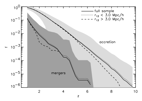
Figure 14: The cumulative growth of the black hole mass as a function of redshift. Shown is the growth of the main progenitor, averaged over each sample, and the growth is divided into growth through accretion and mergers. Black holes of all masses are combined in this Figure. While the solid lines show the full samples, the dotted and dashed lines give black holes in overdense ($r_{13}<3\,h^{-1}$ Mpc) and underdense ($r_{13}\geq 3\,h^{-1}$ Mpc) regions, respectively. For the full sample, the superimposed solid area shows the scatter around the mean.

4.4 BH growth by mergers and accretion in Different Environments

Given the findings from the previous Section, it an important question to see how universal they are. In particular, we now investigate the question of how the environment may affect the modes of black hole growth: accretion and mergers. In order to do this we study the growth of the most massive progenitor of each black hole as a function of redshift, and calculate the contributions to the BH mass due to accretion and mergers separately and how they depend on local environments.

Figure 14 shows the averaged cumulative fraction $f$ of the final BH mass built up through mergers and accretion as a function of redshift (at $z=1$ the sum of the two fractions equals one). The solid lines show the respective fractions for the whole BH sample while the dotted and dashed lines show $f$ in overdense ($r_{13}<3\,h^{-1}$ Mpc and underdense ($r_{13}\geq 3\,h^{-1}$ Mpc) regions respectively. The rms around the mean for the full sample as shaded regions – the scatter for subsamples is of comparable size. Figure 14 shows a mild dependence of the mode of black hole growth with environment. In particular, underdense regions show reduced accretion at $z>3$ and somewhat less mergers at $z<3$ with respect to the high density regions (or the full mean). The reduced merger activity in underdense regions is fully compatible with the evolution of the mass function of haloes in voids (see, for example, Gottlöber et al. 2003 or Goldberg & Vogeley 2004). In voids, the mass function of haloes covers a reduced mass range, and its growth is delayed compared with the growth of the mass function in the $\Lambda$CDM cosmology. It is also expected that the fraction of BH mass contributed by accretion will also be smaller in underdense regions. Overall, the environments affects the mode of BH mass assembly reducing accretion at high–$z$ and mergers at intermediate redshift. However, the final black hole mass fraction at $z=1$ contributed by these two mode remains very similar across dense or underdense environments. Our finding is independent of BH mass – if split up into mass ranges as above the same trend is visible, the only differences between the mass ranges being the times at which the different mass BHs start to form, of course.

A comparison with the mass assembly histories studied in Maulbetsch et al. (2007) is instructive – keep in mind that they use a fixed–radius measure for density, though. Maulbetsch et al. find that for $z=1$ (and higher), average mass aggregation rates of haloes are higher in high–density regions – a finding that agrees with what we see for the black holes in our simulation. Figure 14 can also be compared with Figure 9 in Malbon et al. (2007). Since we do not split the BHs into mass bins Figure 14 is dominated by lower–mass BHs. Taking the different final redshifts into account, Malbon et al.’s Figure 9 and Figure 14 agree qualitatively: For low–mass BHs, accretion is dominant at any redshift (and in any environment). However, it is worthwhile to note how our results indicate that BH growth, both via accretion and mergers, is relevant at redshifts higher than than those seen in Malbon et al. (2007), probably due to the much better mass resolution in our direct simulation.

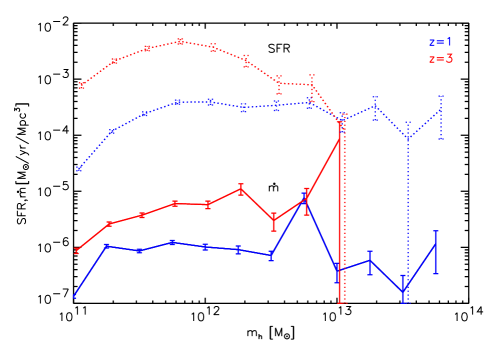
Figure 15: Star formation (dotted lines) and accretion density (solid lines) as a function of halo mass for redshifts $z=1$ (blue) and $z=3$. See main text for full details.

5 Summary and Discussion

We have used high–resolution cosmological hydrodynamic simulations, the first of its kind to fully model massive black holes in cosmological volumes, to investigate the effects of the environment on the growth and evolution of BHs. We have focused our analysis on the BHCosmo simulation and complemented it with a second, larger volume (E6) to achieve higher statistics at high $z$ (see Di Matteo et al. 2007). In this work, we have made used of the full merger trees of each of the black holes in the simulations, comprising four and a half million progenitors in the more than three and a half thousand black holes in the simulation. Our results can be summarized as follows.

• While there is a well–defined correlation between the masses of dark matter haloes and of supermassive black holes at low redshifts, there are some important deviations from the simple hierarchical picture. A large population of the most massive black holes are formed anti–hierarchically, with formation redshifts $z_{f}$ from $z\sim 2$ to $z\sim 4$, while a residual population of the massive BHs is assembled at lower redshift completely consistent with hierarchical assembly.

• Comparing the growth histories of the masses of the most massive black holes and their host haloes’ we have shown that between redshifts of around $z\simeq 6$ and $z\simeq 2$ black holes grow at a much faster rate than their host haloes.

• We have found quite a tight relation between black hole mass $m_{\mbox{\scriptsize{BH}}}$ and host halo mass $m_{\mbox{\scriptsize{h}}}$ at $z=1$, with $m_{\rm BH}\propto m_{\rm h}^{\sim 1.2}$ (for $m_{\mbox{\scriptsize{h}}}\geq 10^{7}$ M_⊙), consistent with observational results by, e.g., Shankar & Mathur (2007). The relation becomes slightly shallower ($m_{\rm BH}\propto m_{\rm h}^{\sim 1.0}$) if we include less massive black holes. The BH accretion rate $\dot{m}$ displays a very similar behaviour ($\dot{m}\propto m_{\rm h}^{\sim 1.0}$), albeit with much larger scatter. In particular, for the most active black holes ($\dot{m}\geq 10^{-2}$ M_⊙/year), the correlation of accretion rate with halo mass disappears.

• Using $r_{13}$, an adaptive measure of the local density, we find that with the exception of satellites, more massive black holes live in more massive haloes, and more massive haloes tend to live in denser environments (roughly $M_{\rm BH}\propto(\rho/\rho_{mean})^{-1.5}$ in Fig. 7). A similar overall density dependency is found for black hole accretion rates, albeit with a far larger scatter. Therefore, in general the largest and most active black holes are found in group environments. Lower mass ($m_{\rm BH}<10^{8}\,\hbox{$\rm\thinspace M_{\odot}$}$) and low accretion black holes are common in all environments, from cluster/group to voids. Accretion rates typically increase with increasing redshift across all environments. The overall decrease in the mean accretion rates is (Fig. 9) accompanied by a shallower density dependency (Fig. 9) with decreasing redshift is in line with observed downsizing in the AGN population (e.g. Steffen et al. 2003, Ueda et al. 2003, Hasinger et al. 2005).

• Figure 11 links accretion rates of black holes and SFRs of their hosts. For fixed accretion (SFR), there is a wide range in SFR (accretion), across the full range of black hole mass ranges. This finding indicates that the relationship between black hole activity and SFR is more complicated than a simple one–to–one correlation (for recent observational work see, e.g., Alonso–Herrero et al. 2007). Consistent with our previous results (Di Matteo et al 2007), the difference in BH accretion and SFR density dependeces further emphasizes a difference in the main triggering mechanisms for quasars and star formation. Even though mergers lead both star formation and black hole accretion, quasar activity is likely to require a major merger. High gas density regions lead to star formation irrespective of a major merger. To further demonstrate this, in Figure 15, we plot the mean accretion rate density (in M_⊙/yr/Mpc³) as a function of halo mass for redshifts $z=1$ (blue solid line) and $z=3$ (red solid line), using Poisson error bars. This illustrates clearly that the peak of the SFR occurs at lower halo masses than those where most quasar activity takes place. Whereas accretion rate tracks the major merger history (effectively the growth of relatively massive halos), the SFR follows the global build up of the relatively low mass halos hosting the most rapidly star-forming galaxies (those with the highest concentration and highest density at high $z$; see also Hopkins et al. 2007). As both SFR and accretion rate decline at lower redshift as a result of the declining gas fraction and merger rates the two better trace each other’s environments. Note that since we do not track the merger histories of either dark matter haloes or of the BH’s host galaxies, we lack the data to distinguish between star formation triggered by a merger/interaction or by quiescent star formation.

• There is a significant number of black holes with masses below $10^{7}$ M_⊙ in haloes of mass $10^{12}$ M_⊙ or less, spread out over the full range of environments, with formation redshifts of 2.5 or higher. Their growth histories are very similar, with only minor differences between them. Mergers are rare (only 20% of these black holes ever experience at least one merger). Thus, at $z=1$ there exists a fairly large population of quite inactive BH, all in small galaxy–sized haloes, across al cosmic environments, including, of course, the most underdense regions, the voids. These low–mass BHs and their slow growth account for the recently observed sample of such AGNs in voids (Constantin et al. 2007).

Measurements of the spatial clustering of quasars as a function of redshift show a rapid increase of QSO bias with redshift (Croom et al. 2005, Myers et al. 2006, Shen et al. 2007, Francke et al. 2008; also see White et al. 2007), from which then minimum halo masses can be estimated. Croom et al. (2005) report a constant halo mass for their 2dF QSOs of $m=(3.0\pm 1.6)\cdot h^{-1}\,10^{12}$ M_⊙, consistent with the results by Shen et al. (2007). We have shown that the range of halo masses for bright AGN in the simulation is broadly consistent with these results (see Fig. 3). Figure 15, also summarizes these results. Note that at both redshifts, the respective high–mass ends are noisy because of the small number of objects. The distributions at both these redshift are not really peaked, but are broadly consistent with the halo masses derived from the quasars in the 2dF and Deep2 survey (Coil et al. 2006). They also agree with the results obtained by Hopkins et al. (2007), whose model shows the same mass range for quasar environments at all redshifts. Please note, that while their model has to rely on using constraints on halo/subhalo and halo occupation distributions from simulations (plus assumptions on what constitutes a major merger), our simulation contains all of these ingredients as additional results.

Regardless of what all of these black holes would do between $z=1$ and $z=0$, their behaviour up to $z=1$ is very consistent with observed observational patterns. For more detailed studies, there clearly is need for further simulations, especially in a larger cosmological volume up to $z=0$. But the basic agreement of the simulations discussed here (and in Di Matteo et al. 2007 and Sijacki et al. 2007) with observations supports the simple model with which the formation and evolution of BHs is treated in the simulation code. Studies of the formation and evolution of BHs in cosmological volumes thus appear feasible.

References

- [1] Adams F.C., Graff D.S., Richstone D.O., 2001, ApJ, 551, 31
- [2] Adelberger K.L., Steidel C.C., 2005, ApJ, 630, 50
- [3] Alonso–Herrero A., Perez–Gonzalez P.G., Rieke G.H., Alexander D.M., Rigby J.R., Papovich C., Donley J.L., Rigopoulou D., 2007, astro-ph/0712.3121 (accepted for publication in ApJ)
- [4] Baker J.G., Centrella J., Choi D.I., Koppitz M., Van Meter J.R., Miller M.C., 2006, ApJ, 653, 93
- [5] Baugh C.M., 2006, Rept.Prog.Phys., 69, 3101
- [6] Benson A.J., Hoyle F., Torres F., Vogeley M.S., 2003, MNRAS, 340, 160
- [7] Blanton M.R., Berlind A.A., 2007, ApJ, 664, 791
- [8] Bondi H., Hoyle F., 1944, MNRAS, 104, 273
- [9] Bondi H., 1952, MNRAS, 112, 195
- [10] Bower R.G., Benson A.J., Malbon R., Helly J.C., Frenk C.S., Baugh C.M., Cole S., Lacey C.G., 2006, MNRAS, 370, 645
- [11] Busha M.T., Evrard A.E., Adams F.C., Wechsler R.H., 2005, MNRAS, 363, 11
- [12] Cattaneo A., Haehnelt M. Rees M.J., 1999, MNRAS, 308, 77
- [13] Coil A.L., Hennawi J.F., Newman J.A., Cooper M.C., Davis M., 2007, ApJ, 654, 115
- [14] Colberg J.M., Sheth R.K., Diaferio A., Gao L., Yoshida N., 2005, MNRAS, 360, 216
- [15] Colberg J.M., Di Matteo T., Springel V., Hernquist L., 2007, in preparation
- [16] Conselice C.J., Chapman S.C., Windhorst R.A., 2003, ApJ, 596, 5
- [17] Constantin A., Vogeley M.S., et al. (?), 2007, ApJ (submitted)
- [18] Cooper M.C., Newman J.A., Madgwick D.S., Gerke B.F., Yan R., Davis M., 2005, ApJ, 634, 833
- [19] Cooper M.C., et al., 2007, astro–ph/0706.4089
- [20] Cowie L.L., Songaila A., Hu E.M., Cohem J.G., 1996, AJ, 112, 839
- [21] Croft R.A.C., Di Matteo T., Springel V., Hernquist L., 2008, arXiv:0803.4003
- [22] Croom S.M., et al., 2005, MNRAS, 356, 415
- [23] Croton D.J., et al., 2006, MNRAS, 365, 11
- [24] Croton D.J., Gao L., White S.D.M., 2007, MNRAS, 374, 1303
- [25] Croton D.J., Farrar G.R., 2008, astro-ph/0801.2771
- [26] Davis M., Efstathiou G., Frenk C.S., White S.D.M., 1985, ApJ, 292, 371
- [27] De Lucia G., Springel V., White S.D.M., Croton D., Kauffmann G., 2006, MNRAS, 366, 499
- [28] De Lucia G., Blaizot J., 2007, MNRAS, 375, 2
- [29] Di Matteo T., Croft R.A.C., Springel V., Hernquist L., 2003, ApJ, 593, 56
- [30] Di Matteo T., Springel V., Hernquist L., 2005, Nature, 433, 604
- [31] Di Matteo T., Colberg J.M., Springel V., Hernquist L., Sijaki D., 2007, submitted to ApJ
- [32] Elbaz D., et al., 2007, A&A, 468, 33
- [33] Fan X., et al., 2003, AJ, 125, 1649
- [34] Ferrarese L., Merritt D., 2000, ApJ, 539, 9
- [35] Ferrarese L., 2002, ApJ, 578, 90
- [36] Francke H., et al., 2008, ApJ, 673, 13
- [37] Gallo E., Treu T., Jacob J., Woo J.H., Marshall P., Antonucci R., 2007, astro-ph/0711.2073
- [38] Gebhardt K., et al., 2000, ApJ, 543, 5
- [39] Goldberg D.M., Vogeley M.S., 2004, ApJ, 605, 1
- [40] Gottlöber S., Lokas E.L., Klypin A., Hoffman Y., 2003, MNRAS, 344, 715
- [41] Granato G.L., Silva L., Monaco P., Panuzzo P., Salucci P., De Zotti G., Danese L., 2001, MNRAS, 324, 757
- [42] Greenstein J.L., Matthews T.A., 1963, Nature, 197, 1041
- [43] Gunn J.E., Gott J.R., 1972, ApJ, 176, 1
- [44] Hasinger G., Miyaji T., Schmidt M., 2005, A&A, 441, 417
- [45] Hatziminaoglou E., Mathez G., Solanes J.M., Manrique A., Salvador-Sole E, 2003, MNRAS, 343, 692
- [46] Heinis S., et al., 2007, Accepted for Publication in the Special GALEX Ap. J. Supplement, December 2007
- [47] Hopkins P.F., Hernquist L., Martini P., Cox T.J., Robertson B., Di Matteo T., Springel V., 2005, ApJ, 625, 71
- [48] Hopkins P.F., Hernquist L., Cox T.J., Keres D., 2007, astro-ph/0706.1243
- [49] Hoffman L., Loeb A., 2006, astro-ph/0612517
- [50] Hoyle F., Lyttleton R.A., 1939, in Proceedings of the Cambridge Philosophical Society (1939), p. 405
- [51] Jiang L., Fan X., Vestergaard M., Kurk J.D., Walter F., Kelly B.C., Strauss M.A., 2007, AJ, in press
- [52] Katz N., Weinberg D.H., Hernquist L., 1996, ApJS, 105, 19
- [53] Kauffmann G., Haehnelt M., 2000, MNRAS, 311, 576
- [54] Kauffmann G., White S.D.M., Heckman T.M., Menard B., Brinchmann J., Charlot S., Tremonti C., Brinkman J., 2004, MNRAS, 353, 713
- [55] Kennicutt R.C., 1989, ApJ, 344, 685
- [56] Kennicutt R.C., 1989, ApJ, 498, 541
- [57] Kurk J.D., et al., 2007, accepted by ApJ
- [58] Lidz A., Hopkins P.F., Cox T.J., Hernquist L., Robertson B., 2006, ApJ, 641, 41
- [59] Lynden-Bell D., 1969, MNRAS, 143, 167
- [60] Malbon R.K., Baugh C.M., Frenk C.S., Lacey C.G., 2007, MNRAS, 382, 1394
- [61] Marconi A., Hunt L.K., 2003, ApJ, 589, L21
- [62] Marulli F., Bonoli S., Branchini E., Moscardini L., Springel V., 2007, astro-ph/0711.2053
- [63] Maulbetsch C., Avila–Reese V., Col n P., Gottlöber S., Khalatyan A., Steinmetz M., 2007, ApJ, 654, 53
- [64] McCarthy I.G., Frenk C.S., Font A.S., Lacey C.G., Bower R.G., Mitchell N.L., Balogh M.L., Theuns T., 2008, MNRAS, 383, 593
- [65] Monaghan J.J., ARA&A, 1992, 30, 543
- [66] Moore B., Quilis V., Bower R., 2000, in Dynamics of Galaxies: from the Early Universe to the Present, 15th IAP meeting held in Paris, France, July 9–13, 1999, Eds.: Francoise Combes, Gary A. Mamon, and Vassilis Charmandaris ASP Conference Series, Vol. 197, ISBN: 1-58381-024-2, p. 363.
- [67] Myers A.D., et al., 2006, ApJ, 638, 622
- [68] Navarro J.F., Frenk C.S., White S.D.M., 1997, ApJ, 490, 493
- [69] Park C., Choi Y.Y., Vogeley M.S., Gott J.R., Blanton M..R., 2007, to appear in ApJ (astro-ph/0611610)
- [70] Pope A., Borys C., Scott D., Conselice C., Dickinson M., Mobasher B., 2005, MNRAS, 358, 149
- [71] Robertson B., Cox T.J., Hernquist L., Franx M., Hopkins P.F., Martini P., Springel V., 2006, ApJ, 641, 21
- [72] Salpeter E., 1964, ApJ, 140, 796
- [73] Schmidt M., 1963, Nature, 197, 1040
- [74] Seljak U., 2002, MNRAS, 334, 797
- [75] Shakura N.I., Sunyaev R.A., 1973, A&A, 24, 337
- [76] Shen Y., et al., 2007, ApJ, 133, 2222
- [77] Shields G.A., Menezes K.L., Massart C.A., Vanden Bout P., 2006, ApJ, 641, 683
- [78] Sijaki D.,, Springel V., Di Matteo T., Hernquist L., 2007, submitted to MNRAS
- [79] Spergel D.N., et al., 2003, ApJS, 148, 175
- [80] Springel V., Hernquist L., 2002, MNRAS, 333, 649
- [81] Springel V., Hernquist L., 2003, MNRAS, 339, 312
- [82] Springel V., Di Matteo T., Hernquist L., 2005, ApJ, 620, L79
- [83] Springel V., 2005, MNRAS, 364, 1105
- [84] Springel V., et al., 2005, Nature, 435, 629
- [85] Steffen A.T., Barger A.J., Cowie L.L., Mushotsky R.F., Yang Y., 2003, ApJ, 596, L23
- [86] Ueda Y., Masayuki A., Ohta K., Miyaji T., 2003, ApJ, 598, 886
- [87] Volonteri M., Haardt F., Madau P.,2003, ApJ, 582, 559
- [88] White M., Martini P., Cohn J.D., 2007, astro-ph/0711.4109
- [89] Woo J.H., Treu T., Malkan M.A., Blandford R.D., 2006, ApJ, 645, 900