Noncoherent Capacity of Underspread Fading Channels

Abstract

We derive bounds on the noncoherent capacity of wide-sense stationary uncorrelated scattering (WSSUS) channels that are selective both in time and frequency, and are underspread, i.e., the product of the channel’s delay spread and Doppler spread is small. For input signals that are peak constrained in time and frequency, we obtain upper and lower bounds on capacity that are explicit in the channel’s scattering function, are accurate for a large range of bandwidth and allow to coarsely identify the capacity-optimal bandwidth as a function of the peak power and the channel’s scattering function. We also obtain a closed-form expression for the first-order Taylor series expansion of capacity in the limit of large bandwidth, and show that our bounds are tight in the wideband regime. For input signals that are peak constrained in time only (and, hence, allowed to be peaky in frequency), we provide upper and lower bounds on the infinite-bandwidth capacity and find cases when the bounds coincide and the infinite-bandwidth capacity is characterized exactly. Our lower bound is closely related to a result by Viterbi (1967).

The analysis in this paper is based on a discrete-time discrete-frequency approximation of WSSUS time- and frequency-selective channels. This discretization explicitly takes into account the underspread property, which is satisfied by virtually all wireless communication channels.

I Introduction and Outline

I-1 Models for fading channels

Channel capacity is a benchmark for the design of any communication system. The techniques used to compute, or at least to bound, channel capacity often provide guidelines for the design of practical systems, e.g., how to best utilize the resources bandwidth and power, and how to design efficient modulation and coding schemes [1, Sec. III.3]. Our goal in this paper is to analyze the capacity of wireless communication channels that are of direct practical importance. We believe that an accurate stochastic model for such channels should take the following aspects into account:

• The channel is selective in time and frequency, i.e., it exhibits memory in frequency and in time, respectively.

• Neither the transmitter nor the receiver knows the instantaneous realization of the channel.

• The peak power of the input signal is limited.

These aspects are important because they arise from practical limitations of real-world communication systems: temporal variations of the environment and multipath propagation are responsible for channel selectivity in time and frequency, respectively [2, 3]; perfect channel knowledge at the receiver is impossible to obtain because channel state information needs to be extracted from the received signal; finally, realizable transmitters are always limited in their peak output power [4]. The above aspects are also fundamental as they significantly impact the behavior of channel capacity: for example, the capacity of a block-fading channel behaves differently from the capacity of a channel that is stationary in time [5]; channel capacity with perfect channel knowledge at the receiver is always larger than the capacity without channel knowledge [6], and the signaling schemes necessary to achieve capacity are also very different in the two cases [1]; finally, a peak constraint on the transmit signal can lead to vanishing capacity in the large-bandwidth limit [7, 8, 9], while without a peak constraint the infinite-bandwidth AWGN capacity can be attained asymptotically [7, 10, 11, 12, 13, 14, 15].

Small scale fading of wireless channels can be sensibly modeled as a stochastic Gaussian linear time-varying (LTV) system [2]; in particular, we base our developments on the widely used wide-sense stationary uncorrelated scattering (WSSUS) model for random LTV channels [16, 12]. Like most models for real-world channels, the WSSUS model is time continuous; however, almost all tools for information-theoretic analysis of noisy channels require a discretized representation of the channel’s input-output relation. Several approaches to discretize random LTV channels are proposed in the literature, e.g., sampling [8, 16, 17] or basis expansion [18, 19]; all these discretized models incur an approximation error with respect to the continuous-time WSSUS model that is often difficult to quantify. As virtually all wireless channels of practical interest are underspread, i.e., the product of maximum delay and maximum Doppler shift is small, we build our information-theoretic analysis upon a discretization of LTV channels, proposed by Kozek [20], that explicitly takes into account the underspread property to minimize the approximation error in the mean-square sense.

I-2 Capacity of noncoherent WSSUS channels

Throughout the paper, we assume that both the transmitter and receiver know the channel law but both are ignorant of the channel realization, a setting often called noncoherent. In the following, we refer to channel capacity in the noncoherent setting simply as “capacity”. In contrast, in the coherent setting the receiver is also assumed to know the channel realization perfectly; the corresponding capacity is termed coherent capacity.

A general closed-form expression for the capacity of Rayleigh-fading channels is not known, even if the channel is memoryless [22]. However, several asymptotic results are available. If only a constraint on the average transmitted power is imposed, the AWGN capacity can be achieved in the infinite-bandwidth limit also in the presence of fading. This result is quite robust, as it holds for a wide variety of channel models [7, 10, 11, 12, 13, 14, 15]. Verdú showed that flash signaling, which implies unbounded peak power of the input signal, is necessary and sufficient to achieve the infinite-bandwidth AWGN capacity on block-memoryless fading channels [14]; a form of flash signaling is also infinite-bandwidth optimal for the more general time- and frequency-selective channel model used in the present paper [15]. In contrast, if the peakiness of the input signal is restricted, the infinite-bandwidth capacity behavior of most fading channels changes drastically, and the limit depends on the type of peak constraint imposed [7, 8, 9, 13, 23]. In this paper, we shall distinguish between a peak constraint in time and a peak constraint in time and frequency.

Peak constraint in time

No closed-form capacity expression, not even in the infinite-bandwidth limit, seems to exist to date for time- and frequency-selective WSSUS channels. Viterbi’s analysis [23] provides a result that can be interpreted as a lower bound on the infinite-bandwidth capacity of time- and frequency-selective channels. This lower bound is in the form of the infinite-bandwidth AWGN capacity minus a penalty term that depends on the channel’s power-Doppler profile [16]. For channels that are time selective but frequency flat, structurally similar expressions were found for the infinite-bandwidth capacity [24, 25] and for the capacity per unit energy [26].

Peak constraint in time and frequency

Although a closed-form capacity expression valid for all bandwidths is not available, it is known that the infinite-bandwidth capacity is zero for various channel models [7, 8, 9]. This asymptotic capacity behavior implies that signaling schemes that spread the transmit energy uniformly across time and frequency perform poorly in the large-bandwidth regime. Even more useful for performance assessment would be capacity bounds for finite bandwidth. For frequency-flat time-selective channels, such bounds can be found in [27, 28], while for the more general time- and frequency-selective case treated in the present paper, upper bounds seem to exist only on the rates achievable with particular signaling schemes, namely for orthogonal frequency-division multiplexing (OFDM) with constant-modulus symbols [29], and for multiple-input multiple-output (MIMO) OFDM with unitary space-frequency codes over frequency-selective block-fading channels [30].

I-3 Contributions

We use the discrete-time discrete-frequency approximation of continuous-time underspread WSSUS channels proposed in [20], to obtain the following results:

• We derive upper and lower bounds on capacity under a constraint on the average power and under a peak constraint in both time and frequency. These bounds are valid for any bandwidth, are explicit in the channel’s scattering function, and generalize the results on achievable rates in [29]. In particular, our bounds allow to coarsely identify the capacity-optimal bandwidth for a given peak constraint and a given scattering function.

• Under the same peak constraint in time and frequency, we find the first-order Taylor series expansion of channel capacity in the limit of infinite bandwidth. This result extends the asymptotic capacity analysis for frequency-flat time-selective channels in [28] to channels that are selective in both time and frequency.

• In the infinite-bandwidth limit and for transmit signals that are peak-constrained in time only, we recover Viterbi’s capacity lower bound [23]. In addition, we derive an upper bound that is shown to coincide with the lower bound for a specific class of channels; hence, the infinite-bandwidth capacity for this class of channels is established.

The results in this paper rely on several flavors of Szegö’s theorem on the asymptotic eigenvalue distribution of Toeplitz matrices [31, 32]; in particular, we use various extensions of Szegö’s theorem to two-level Toeplitz matrices, i.e., block-Toeplitz matrices that have Toeplitz blocks [33, 34]. Another key ingredient for several of our proofs is the relation between mutual information and minimum mean-square error (MMSE) discovered recently by Guo et al. [35]. Furthermore, we use a property of the information divergence of orthogonal signaling schemes derived by Butman and Klass [36].

I-4 Notation

Uppercase boldface letters denote matrices and lowercase boldface letters designate vectors. The superscripts ^T, ^∗, and ^H stand for transposition, element-wise conjugation, and Hermitian transposition, respectively. For two matrices $\mathbf{A}$ and $\mathbf{B}$ of appropriate dimensions, the Hadamard product is denoted as $\mathbf{A}\operatorname{\odot}\mathbf{B}$. We designate the identity matrix of dimension $N\times N$ as $\mathbf{I}_{N}$ and the all-zero vector of appropriate dimension as $\mathbf{0}$. We let $\mathrm{diag}\mathopen{}\left(\mathbf{x}\right)$ denote a diagonal square matrix whose main diagonal contains the elements of the vector $\mathbf{x}$. The determinant, trace, and rank of the matrix $\mathbf{X}$ are denoted as $\det(\mathbf{X})$, $\operatorname{tr}(\mathbf{X})$, and $\operatorname{rank}(\mathbf{X})$, respectively, and $\lambda_{i}(\mathbf{X})$ is the $i$th eigenvalue of a square matrix $\mathbf{X}$. The function $\delta(x)$ is the Dirac distribution, and $\delta[n]$ is defined as $\delta[0]=1$ and $\delta[n]=0$ for all $n\neq 0$. All logarithms are to the base $e$. The real part of the complex number $z$ is denoted $\Re\{z\}$. We write $\mathcal{A}-\mathcal{B}$ for the set difference between the sets $\mathcal{A}$ and $\mathcal{B}$. For two functions $f(x)$ and $g(x)$, the notation $f(x)=\operatorname{\mathit{o}}\mathopen{}\left(g(x)\right)$ for $x\to 0$ means that $\lim_{x\to 0}f(x)/g(x)=0$. With $\lfloor x\rfloor$ we denote the largest integer smaller or equal to $x\in\mathbb{R}$. A signal is an element of the Hilbert space $\mathcal{L}^{2}$ of square integrable functions. The inner product between two signals $f(x)$ and $g(x)$ is denoted as $\langle f,g\rangle=\int_{-\infty}^{\infty}f(x)g^{*}(x)dx$. For a random variable (RV) $x$ with distribution $Q_{x}$, we write $x\sim Q_{x}$. We denote expectation by $\operatorname{\mathbb{E}}\mathopen{}\left[\cdot\right]$, and use the notation $\operatorname{\mathbb{E}}_{x}\mathopen{}\left[\cdot\right]$ to stress that the expectation is taken with respect to the RV $x$. We write $D\mathopen{}\left(Q_{x}\|Q_{y}\right)$ for the Kullback-Leibler (KL) divergence between the two distributions $Q_{x}$ and $Q_{y}$. Finally, $\mathcal{CN}(\mathbf{m},\mathbf{R})$ stands for the distribution of a jointly proper Gaussian (JPG) random vector with mean $\mathbf{m}$ and covariance matrix $\mathbf{R}$.

II Channel and System Model

A channel model needs to strike a balance between generality, accuracy, engineering relevance, and mathematical tractability. In the following, we start from the classical WSSUS model for LTV channels [16, 12] because it is a fairly general, yet accurate and mathematically tractable model that is widely used. This model has a continuous-time input-output relation, which is difficult to use as a basis for information-theoretic studies. However, if the channel is underspread it is possible to closely approximate the original WSSUS input-output relation by a discretized input-output relation that is especially suited for the derivation of capacity bounds. In particular, the bounds we derive in this paper can be directly related to the underlying continuous-time WSSUS channel as they are explicit in its scattering function.

II-A Time- and Frequency-Selective Underspread Fading Channels

II-A1 The channel operator

A wireless channel can be described as a linear operator $\operatorname{\mathbb{H}}:\mathcal{L}^{2}\to\mathcal{R}_{\operatorname{\mathbb{H}}}$ that maps an input signal $x(t)$ into an output signal $r(t)\in\mathcal{R}_{\operatorname{\mathbb{H}}}$, where $\mathcal{R}_{\operatorname{\mathbb{H}}}\subset\mathcal{L}^{2}$ denotes the range space of $\operatorname{\mathbb{H}}$ [37]. The corresponding noise-free input-output relation is then $r(t)=(\operatorname{\mathbb{H}}\!x)(t)$.

It is sensible to model wireless channels as random, for one because a deterministic description of the physical propagation environment is too complex in most cases of practical interest, and second because a stochastic description is much more robust, in the sense that systems designed on the basis of a stochastic channel model can be expected to work in a variety of different propagation environments [3]. Consequently, we assume that $\operatorname{\mathbb{H}}$ is a random operator.

II-A2 System functions

Because communication takes place over a finite bandwidth and a finite time duration, we can assume that each realization of $\operatorname{\mathbb{H}}$ is a Hilbert-Schmidt operator [38, 39]. Hence, the noise-free input-output relation of the LTV channel can be written as[38, p. 1083]

$$r(t)=\bigl{(}\operatorname{\mathbb{H}}\!x\bigr{)}(t)=\int_{t^{\prime}}k_{\operatorname{\mathbb{H}}}(t,t^{\prime})x(t^{\prime})dt^{\prime}$$ (1)

where the kernel $k_{\operatorname{\mathbb{H}}}(t,t^{\prime})$ can be interpreted as the channel response at time $t$ to a Dirac impulse at time $t^{\prime}$. Instead of two variables that denote absolute time, it is common in the engineering literature to use absolute time $t$ and delay $\tau$. This leads to the time-varying impulse response $h_{\operatorname{\mathbb{H}}}(t,\tau)=k_{\operatorname{\mathbb{H}}}(t,t-\tau)$ and the corresponding noise-free input-output relation [16]

$$r(t)=\int_{\tau}h_{\operatorname{\mathbb{H}}}(t,\tau)x(t-\tau)d\tau.$$ (2)

Two more system functions that will be important in the following developments are the time-varying transfer function

$$L_{\operatorname{\mathbb{H}}}(t,f) =\int_{\tau}h_{\operatorname{\mathbb{H}}}(t,\tau)e^{-j2\pi f\tau}d\tau$$ (3)

and the spreading function

$$S_{\operatorname{\mathbb{H}}}(\nu,\tau) =\int_{t}h_{\operatorname{\mathbb{H}}}(t,\tau)e^{-j2\pi\nu t}dt=\iint_{t\>f}L_{\operatorname{\mathbb{H}}}(t,f)e^{-j2\pi(\nu t-\tau\!f)}dtdf.$$ (4)

In particular, if we rewrite the input-output relation (2) in terms of the spreading function $S_{\operatorname{\mathbb{H}}}(\nu,\tau)$ as

$$r(t)=\iint_{\nu\>\tau}S_{\operatorname{\mathbb{H}}}(\nu,\tau)x(t-\tau)e^{j2\pi t\nu}d\tau d\nu$$ (5)

we obtain an intuitive physical interpretation: the output signal $r(t)$ is a weighted superposition of copies of the input signal $x(t)$ that are shifted in time by the delay $\tau$ and in frequency by the Doppler shift $\nu$.

II-A3 Stochastic characterization and WSSUS assumption

For mathematical tractability, we need to make additional assumptions on the system functions. First, we assume that $L_{\operatorname{\mathbb{H}}}(t,f)$ is a zero-mean JPG random process in $t$ and $f$. Indeed, the Gaussian distribution is empirically supported for narrowband channels [2], and even ultrawideband (UWB) channels with bandwidth up to several gigahertz can be modeled as Gaussian distributed [40]. By virtue of the Gaussian assumption, $L_{\operatorname{\mathbb{H}}}(t,f)$ is completely characterized by its correlation function. Yet, this correlation function is four-dimensional in general and thus difficult to work with. A further simplification is possible if we assume that the channel process is wide-sense stationary in time $t$ and uncorrelated in delay $\tau$, the so-called WSSUS assumption [16]. As a consequence, $L_{\operatorname{\mathbb{H}}}(t,f)$ is wide-sense stationary both in time $t$ and frequency $f$, or, equivalently, $S_{\operatorname{\mathbb{H}}}(\nu,\tau)$ is uncorrelated in Doppler $\nu$ and delay $\tau$ [16]:

$$\operatorname{\mathbb{E}}\mathopen{}\left[L_{\operatorname{\mathbb{H}}}(t,f)L_{\operatorname{\mathbb{H}}}^{*}(t^{\prime},f^{\prime})\right] =R_{\operatorname{\mathbb{H}}}(t-t^{\prime},f-f^{\prime})$$

$$\operatorname{\mathbb{E}}\mathopen{}\left[S_{\operatorname{\mathbb{H}}}(\nu,\tau)S_{\operatorname{\mathbb{H}}}^{*}(\nu^{\prime},\tau^{\prime})\right] =C_{\operatorname{\mathbb{H}}}(\nu,\tau)\delta(\nu-\nu^{\prime})\delta(\tau-\tau^{\prime}).$$

The function $R_{\operatorname{\mathbb{H}}}(t,f)$ is called the channel’s (time-frequency) correlation function, and $C_{\operatorname{\mathbb{H}}}(\nu,\tau)$ is called the scattering function of the channel $\operatorname{\mathbb{H}}$. The two functions are related by a two-dimensional Fourier transform,

$$C_{\operatorname{\mathbb{H}}}(\nu,\tau)=\iint_{t\>f}R_{\operatorname{\mathbb{H}}}(t,f)e^{-j2\pi(\nu t-\tau\!f)}dtdf.$$ (6)

As $R_{\operatorname{\mathbb{H}}}(t,f)$ is stationary in $t$ and $f$, $C_{\operatorname{\mathbb{H}}}(\nu,\tau)$ is nonnegative and real-valued for all $\nu$ and $\tau$, and can be interpreted as the spectrum of the channel process. The power-delay profile of $\operatorname{\mathbb{H}}$ is defined as

$$p_{\operatorname{\mathbb{H}}}(\tau) =\int_{\nu}C_{\operatorname{\mathbb{H}}}(\nu,\tau)d\nu$$

and the power-Doppler profile as

$$q_{\operatorname{\mathbb{H}}}(\nu) =\int_{\tau}C_{\operatorname{\mathbb{H}}}(\nu,\tau)d\tau.$$

The WSSUS assumption is widely used in wireless channel modeling [16, 12, 2, 1, 41, 42]. It is in good agreement with measurements of tropospheric scattering channels [12], and provides a reasonable model for many types of mobile radio channels [43, 44, 45], at least over a limited time duration and bandwidth [16]. Furthermore, the scattering function can be directly estimated from measured data [46, 47], so that capacity expressions and bounds that explicitly depend on the channel’s scattering function can be evaluated for many channels of practical interest.

Formally, the WSSUS assumption is mathematically incompatible with the requirement that $\operatorname{\mathbb{H}}$ is of Hilbert-Schmidt type, or, equivalently, that the system functions are square integrable, because stationarity in time $t$ and frequency$f$ of $L_{\operatorname{\mathbb{H}}}(t,f)$ implies that $L_{\operatorname{\mathbb{H}}}(t,f)$ cannot decay to zero for $t\to\infty$ and $f\to\infty$. Similarly to the engineering model of white noise, this incompatibility is a mathematical artifact and not a problem of real-world wireless channels: in fact, every communication system transmits over a finite time duration and over a finite bandwidth. We believe that the simplification the WSSUS assumption entails justifies this mathematical inconsistency.

II-B The Underspread Assumption and its Consequences

Because the velocity of the transmitter, of the receiver, and of the objects in the propagation environment is limited, so is the maximum Doppler shift $\nu_{0}$ experienced by the transmitted signal. We also assume that the maximum delay is strictly smaller than $2\tau_{0}$. For simplicity and without loss of generality, throughout this paper, we consider scattering functions that are centered at $\tau=0$ and $\nu=0$, i.e., we remove any overall fixed delay and Doppler shift. The assumptions of limited Doppler shift and delay then imply that the scattering function is supported on a rectangle of spread $\Delta_{\operatorname{\mathbb{H}}}=4\nu_{0}\tau_{0}$,

$$C_{\operatorname{\mathbb{H}}}(\nu,\tau)=0\quad\text{for }(\nu,\tau)\notin[-\nu_{0},\nu_{0}]\times[-\tau_{0},\tau_{0}].$$ (7)

Condition (7) in turn implies that the spreading function $S_{\operatorname{\mathbb{H}}}(\nu,\tau)$ is also supported on the same rectangle with probability 1 (w.p.1). If $\Delta_{\operatorname{\mathbb{H}}}<1$, the channel is said to be underspread [16, 12, 20]. Virtually all channels in wireless communication are highly underspread, with $\Delta_{\operatorname{\mathbb{H}}}\approx 10^{-3}$ for typical land-mobile channels and as low as $10^{-7}$ for some indoor channels with restricted mobility of the terminals [49, 50, 51]. The underspread property of typical wireless channels is very important, first because only (deterministic) underspread channels can be completely identified from measurements [52, 53], and second because underspread channels have a well-structured set of approximate eigenfunctions that can be used to discretize the channel operator, as described next.

II-B1 Approximate diagonalization of underspread channels

As $\operatorname{\mathbb{H}}$ is a Hilbert-Schmidt operator, its kernel can be expressed in terms of its positive singular values $\{\sigma_{i}\}$, its left singular functions $\{u_{i}(t)\}$, and its right singular functions $\{v_{i}(t)\}$ [37, Th. 6.14.1], according to

$$k_{\operatorname{\mathbb{H}}}(t,t^{\prime})=\sum_{i=-\infty}^{\infty}\sigma_{i}u_{i}(t)v^{*}_{i}(t^{\prime}).$$ (8)

We denote by $\mathcal{N}_{\operatorname{\mathbb{H}}}$ the null space of $\operatorname{\mathbb{H}}$, i.e., the space of input signals that the channel maps onto $0$. The set $\{v_{i}(t)\}$ is an orthonormal basis for the linear span of $\mathcal{L}^{2}-\mathcal{N}_{\operatorname{\mathbb{H}}}$, and $\{u_{i}(t)\}$ is an orthonormal basis for the range space $\mathcal{R}_{\operatorname{\mathbb{H}}}$. Any input signal in $\mathcal{N}_{\operatorname{\mathbb{H}}}$ is of no utility for communication purposes; the remaining input signals in the linear span of $\mathcal{L}^{2}-\mathcal{N}_{\operatorname{\mathbb{H}}}$, which we denote in the remainder of the paper as input space, can be completely characterized by their projections onto the set $\{v_{i}(t)\}$. Similarly, the output signal $r(t)=(\operatorname{\mathbb{H}}x)(t)$ is completely described by its projections onto the set $\{u_{i}(t)\}$. These projections together with the kernel decomposition (8) yield a countable set of scalar input-output relations, which we refer to as the diagonalization of $\operatorname{\mathbb{H}}$.

Because the right and left singular functions depend on the realization of $\operatorname{\mathbb{H}}$, diagonalization requires perfect channel knowledge. But this knowledge is not available in the noncoherent setting. In contrast, if the singular functions of the random channel $\operatorname{\mathbb{H}}$ did not depend on its particular realization, we could diagonalize $\operatorname{\mathbb{H}}$ without knowledge of the channel realization. This is the case, for example, for random linear time-invariant (LTI) channels, where complex sinusoids are always eigenfunctions, independently of the realization of the channel’s impulse response. Fortunately, the singular functions of underspread random LTV channels can be well approximated by deterministic functions. More precisely, an underspread channel $\operatorname{\mathbb{H}}$ has the following properties [20]:

1. All realizations of the underspread channel $\operatorname{\mathbb{H}}$ are approximately normal, so that the singular value decomposition (8) can be replaced by an eigenvalue decomposition.

2. Any deterministic unit-energy signal $g(t)$ that is well localized in time and frequency is an approximate eigenfunction of $\operatorname{\mathbb{H}}$ in the mean-square sense, i.e., the mean-square error $\operatorname{\mathbb{E}}\mathopen{}\left[\lVert\langle\operatorname{\mathbb{H}}g,g\rangle g-\operatorname{\mathbb{H}}g\rVert^{2}\right]$ is small if $\operatorname{\mathbb{H}}$ is underspread. This error can be further reduced by an appropriate choice of $g(t)$, where the choice depends on the scattering function $C_{\operatorname{\mathbb{H}}}(\nu,\tau)$.

3. If $g(t)$ is an approximate eigenfunction as defined in the previous point, then so is $g_{(\alpha,\beta)}(t)=g(t-\alpha)e^{j2\pi\beta t}$ for any time shift $\alpha\in\mathbb{R}$ and any frequency shift $\beta\in\mathbb{R}$.

4. For any $(\alpha,\beta)$, the time-varying transfer function $L_{\operatorname{\mathbb{H}}}(\alpha,\beta)$ is an approximate eigenvalue of $\operatorname{\mathbb{H}}$ corresponding to the approximate eigenfunction $g_{(\alpha,\beta)}(t)$, in the sense that the mean-square error $\operatorname{\mathbb{E}}\bigl{[}\left\lvert\langle\operatorname{\mathbb{H}}g_{(\alpha,\beta)},g_{(\alpha,\beta)}\rangle-L_{\operatorname{\mathbb{H}}}(\alpha,\beta)\right\rvert^{2}\bigr{]}$ is small.

We use these properties of underspread operators to construct an approximation $\widetilde{\operatorname{\mathbb{H}}}$ of the random channel $\operatorname{\mathbb{H}}$ that has a well-structured set of deterministic eigenfunctions. The errors incurred by this approximation are discussed in detail in Appendix A. We then diagonalize this approximating operator and exclusively consider the corresponding discretized input-output relation in the reminder of the paper. Property 1, the approximate normality of $\operatorname{\mathbb{H}}$, together with Property 2 implies that the kernel of the approximating operator $\widetilde{\operatorname{\mathbb{H}}}$ can be synthesized as $\sum_{i=-\infty}^{\infty}\lambda_{i}z_{i}(t)z^{*}_{i}(t^{\prime}),$ where, differently from (8), the $\lambda_{i}$ are now random eigenvalues instead of random singular values, and the $z_{i}(t)$ constitute a set of deterministic orthonormal eigenfunctions instead of random singular functions. Property 2 means that we are at liberty to choose the approximate eigenfunctions $z_{i}(t)$ among all signals that are well localized in time and frequency. In particular, we would like the resulting approximating kernel to be convenient to work with and the approximate eigenfunctions $z_{i}(t)$ easy to implement, as discussed in Section II-B3; therefore, we choose the set of approximate eigenfunctions to be highly structured. By Property 3, it is possible to use time- and frequency-shifted versions of a single well-localized prototype function $g(t)$ as eigenfunctions. Furthermore, because the support of $S_{\operatorname{\mathbb{H}}}(\nu,\tau)$ is strictly limited in Doppler $\nu$ and delay $\tau$, it follows from the sampling theorem and the Fourier transform relation (4) that the samples $L_{\operatorname{\mathbb{H}}}(kT,nF)$, taken on a rectangular grid with $T\leq 1/(2\nu_{0})$ and $F\leq 1/(2\tau_{0})$, are sufficient to characterize $L_{\operatorname{\mathbb{H}}}(t,f)$ exactly. Hence, we take as our set of approximate eigenfunctions the so-called Weyl-Heisenberg set $\{g_{k,n}(t)\}$, where $g_{k,n}(t)=g(t-kT)e^{j2\pi nFt}$ are orthonormal signals. The requirement that the $g_{k,n}(t)$ are orthonormal and at the same time well localized in time and frequency implies $TF>1$ [54], as a consequence of the Balian-Low theorem [55, Ch. 8]. Large values of the product $TF$ allow for better time-frequency localization of $g(t)$, but result in a loss of dimensions in signal space compared with the critically sampled case $TF=1$. The Nyquist condition $T\leq 1/(2\nu_{0})$ and $F\leq 1/(2\tau_{0})$ can be readily satisfied for all underspread channels.

The samples $L_{\operatorname{\mathbb{H}}}(kT,nF)$ are approximate eigenvalues of $\operatorname{\mathbb{H}}$ by Property 4; hence, our choice of approximate eigenfunctions results in the following approximating eigenvalue decomposition for $k_{\operatorname{\mathbb{H}}}(t,t^{\prime})$

$$k_{\operatorname{\mathbb{H}}}(t,t^{\prime})\approx k_{\widetilde{\operatorname{\mathbb{H}}}}(t,t^{\prime})=\sum_{k=-\infty}^{\infty}\sum_{n=-\infty}^{\infty}L_{\operatorname{\mathbb{H}}}(kT,nF)g_{k,n}(t)g_{k,n}^{*}(t^{\prime})$$ (9)

where $k_{\widetilde{\operatorname{\mathbb{H}}}}(t,t^{\prime})$ denotes the kernel of the approximating operator $\widetilde{\operatorname{\mathbb{H}}}$. For $TF>1$, the Weyl-Heisenberg set $\{g_{k,n}(t)\}$ is not complete in $\mathcal{L}^{2}$ [54, Th. 8.3.1]. Therefore, the null space of $\widetilde{\operatorname{\mathbb{H}}}$ is nonempty. As $k_{\widetilde{\operatorname{\mathbb{H}}}}(t,t^{\prime})$ is only an approximation of $k_{\operatorname{\mathbb{H}}}(t,t^{\prime})$, this null space might differ from $\mathcal{N}_{\operatorname{\mathbb{H}}}$. Similarly, the range space of $\widetilde{\operatorname{\mathbb{H}}}$ might differ from $\mathcal{R}_{\operatorname{\mathbb{H}}}$. The characterization of the difference between these spaces is an important open problem.

II-B2 Canonical characterization of signaling schemes

The approximating random channel operator $\widetilde{\operatorname{\mathbb{H}}}$ has a highly structured set of deterministic orthonormal eigenfunctions. We can, therefore, diagonalize the input-output relation of the approximating channel without the need for channel knowledge at both transmitter and receiver. Any input signal $x(t)$ that lies in the input space of the approximating operator is uniquely characterized by its projections onto the set $\{g_{k,n}(t)\}$. All physically realizable transmit signals are effectively band limited. As the prototype function $g(t)$ is well concentrated in frequency by construction, we can model the effective band limitation of $x(t)$ by using only a finite number of slots $N$ in frequency. The resulting transmitted signal

$$x(t)=\sum_{k=-\infty}^{\infty}\sum_{n=0}^{N-1}\underbrace{\langle x,g_{k,n}\rangle}_{=x[k,n]}g_{k,n}(t)$$ (10)

then has effective bandwidth $W=NF$. We call the coefficient $x[k,n]$ the transmit symbol in the time-frequency slot $(k,n)$. The received signal can be expanded in the same basis. To compute the resulting projections, we substitute $k_{\widetilde{\operatorname{\mathbb{H}}}}(t,t^{\prime})$ and the canonical input signal (10) into the integral input-output relation (1), add white Gaussian noise $w(t)$, and project the resulting noisy received signal $y(t)=(\widetilde{\operatorname{\mathbb{H}}}x)(t)+w(t)$ onto the functions $\{g_{k,n}(t)\}$, i.e.,

$$\begin{split}y[k,n]&=\langle y,g_{k,n}\rangle=\langle\widetilde{\operatorname{\mathbb{H}}}x,g_{k,n}\rangle+\underbrace{\langle w,g_{k,n}\rangle}_{w[k,n]}\\ &=\sum_{k^{\prime},n^{\prime}}x[k^{\prime},n^{\prime}]\langle\widetilde{\operatorname{\mathbb{H}}}g_{k^{\prime},n^{\prime}},g_{k,n}\rangle+w[k,n]\\ &=\underbrace{L_{\operatorname{\mathbb{H}}}(kT,nF)}_{h[k,n]}x[k,n]+w[k,n]\end{split}$$ (11)

for all time-frequency slots $(k,n)$. The last step in (11) follows from the orthonormality of the set $\{g_{k,n}(t)\}$. Orthonormality also implies that the discretized noise signal $w[k,n]$ is JPG, independent and identically distributed (i.i.d.) over time $k$ and frequency $n$; for convenience, we normalize the noise variance so that $w[k,n]\sim\mathcal{CN}(0,1)$ for all $k$ and $n$. The diagonalized input-output relation (11) is completely generic, i.e., it is not limited to a specific signaling scheme.

II-B3 OFDM interpretation of the approximating channel model

The canonical signaling scheme (10) and the corresponding discretized input-output relation (11), are not just tools to analyze channel capacity, but also lead to a practical transmission system. The decomposition of the channel input signal (10) can be interpreted as pulse-shaped (PS) OFDM [56], where discrete data symbols $x[k,n]$ are modulated onto a set of orthogonal signals, indexed by $k$ and $n$. In addition, this perspective leads to an operational interpretation of the error incurred when approximating $k_{\operatorname{\mathbb{H}}}(t,t^{\prime})$ as in (9). The time- and frequency-dispersive nature of LTV channels leads to intersymbol interference (ISI) and intercarrier interference (ICI) in the received PS-OFDM signal. This is apparent if we project $r(t)$ onto the function $g_{k,n}(t)$:

$$\langle r,g_{k,n}\rangle=\langle\operatorname{\mathbb{H}}\!x,g_{k,n}\rangle=\sum_{k^{\prime}=-\infty}^{\infty}\sum_{n^{\prime}=0}^{N-1}x[k^{\prime},n^{\prime}]\langle\operatorname{\mathbb{H}}\!g_{k^{\prime},n^{\prime}},g_{k,n}\rangle\\ =\langle\operatorname{\mathbb{H}}\!g_{k,n},g_{k,n}\rangle x[k,n]+\mathop{\sum_{k^{\prime}=-\infty}^{\infty}\sum_{n^{\prime}=0}^{N-1}}_{(k^{\prime},n^{\prime})\neq(k,n)}x[k^{\prime},n^{\prime}]\langle\operatorname{\mathbb{H}}\!g_{k^{\prime},n^{\prime}},g_{k,n}\rangle.$$ (12)

The second term on the right-hand side (RHS) of (12) corresponds to ISI and ICI, while the first term is the desired signal; we can approximate the first term as $L_{\operatorname{\mathbb{H}}}(kT,nF)x[k,n]$ by Property 4. Comparison of (11) and (12) then shows that the input-output relation (11), which results from the approximation (9), can be interpreted as PS-OFDM transmission over the original channel $\operatorname{\mathbb{H}}$ if all ISI and ICI terms are neglected.

With proper design of the prototype signal $g(t)$ and choice of the grid parameters $T$ and $F$, both ISI and ICI can be reduced [56, 57, 58]. The larger the product $TF$, the more effective the reduction in ISI and ICI, as discussed in Appendix A. Heuristically, a good compromise between loss of dimensions in signal space and reduction of the interference terms seems to result for $TF\simeq 1.2$ [56, 58]. The cyclic prefix (CP) in a conventional CP-OFDM system incurs a similar dimension loss.

In (72), we provide an upper bound on mean-square energy of the interference term in (12), and show how this upper bound can be minimized by a careful choice of the signal $g(t)$ and of the grid parameters $T$ and $F$ [20, 17, 58]. For general scattering functions, the optimization of the triple $\{g(t),T,F\}$ needs to be performed numerically; a general guideline is to choose $T$ and $F$ such that (see Appendix A)

$$\frac{T}{F}=\frac{\tau_{0}}{\nu_{0}}.$$ (13)

To summarize, in this section we constructed an approximation $\widetilde{\operatorname{\mathbb{H}}}$ of the random linear operator $\operatorname{\mathbb{H}}$ on the basis of the underspread property. The kernel of the approximating operator is synthesized from the Weyl-Heisenberg set $\{g_{k,n}(t)\}$ as in (9), so that $\{g_{k,n}(t)\}$ is an orthonormal basis for the input space and the range space of $\widetilde{\operatorname{\mathbb{H}}}$. The decomposition of the input signal (10) can be interpreted as PS-OFDM: this interpretation sheds light on one of the errors resulting from the approximation (9). Finally, an important open problem is the characterization of the difference between the input spaces of $\operatorname{\mathbb{H}}$ and $\widetilde{\operatorname{\mathbb{H}}}$, and between the range spaces of $\operatorname{\mathbb{H}}$ and $\widetilde{\operatorname{\mathbb{H}}}$.

II-C Linear Time-Invariant and Linear Frequency-Invariant Channels

The properties of LTV underspread channels we listed in Section II-B are similar to the properties of LTI and linear frequency-invariant (LFI) channels: both LTI and LFI channel operators are normal and have a well-structured set of deterministic eigenfunctions (sinusoids parametrized by frequency for LTI channels, and Dirac functions parametrized by time for LFI channels), with corresponding eigenvalues equal to the samples of a channel system function (e.g., the transfer function in the LTI case). Intuitively, LTI and LFI channels are limiting cases within the class of LTV channels analyzed in this section; in fact, an LTV channel reduces to an LTI channel when $\nu_{0}=0$, and to an LFI channel when $\tau_{0}=0$. Both LTI and LFI channels are then underspread, according to our definition. Yet, since LTI and LFI channel operators are not of Hilbert-Schmidt type [59, App. A], the kernel diagonalization presented in Section II-B does not apply to these two classes of channels; consequently, the capacity bounds we derive in Sections III and IV do not reduce to capacity bounds for the LTI or the LFI case when $\nu_{0}=0$ or $\tau_{0}=0$, respectively.

Quasi-LTI channels, i.e., channels that are slowly time varying ($\nu_{0}$ small but positive), and quasi-LFI channels, i.e., channels that are slowly frequency varying ($\tau_{0}$ small but positive), can instead be approximately diagonalized as described in Section II-B, as long as they are underspread.

II-D Discrete-Time Discrete-Frequency Input-Output Relation

The discrete-time discrete-frequency channel coefficients $\{h[k,n]\}$ constitute a two-dimensional discrete-parameter stationary random process that is JPG with zero mean and correlation function

$$R_{\operatorname{\mathbb{H}}}[k,n]=\operatorname{\mathbb{E}}\mathopen{}\left[h[k^{\prime}+k,n^{\prime}+n]h^{*}[k^{\prime},n^{\prime}]\right]=\operatorname{\mathbb{E}}\mathopen{}\left[L_{\operatorname{\mathbb{H}}}\bigl{(}(k^{\prime}+k)T,(n^{\prime}+n)F\bigr{)}L_{\operatorname{\mathbb{H}}}^{*}(k^{\prime}T,n^{\prime}F)\right].$$ (14)

The two-dimensional power spectral density of $\{h[k,n]\}$ is defined as

$$c(\theta,\varphi)=\sum_{k=-\infty}^{\infty}\sum_{n=-\infty}^{\infty}R_{\operatorname{\mathbb{H}}}[k,n]e^{-j2\pi(k\theta-n\varphi)},\quad\left\lvert\theta\right\rvert,\left\lvert\varphi\right\rvert\leq 1/2.$$ (15)

We shall often need the following expression for $c(\theta,\varphi)$ in terms of the scattering function $C_{\operatorname{\mathbb{H}}}(\nu,\tau)$:

$$\begin{split}c(\theta,\varphi)&\stackrel{{\scriptstyle(a)}}{{=}}\sum_{k=-\infty}^{\infty}\sum_{n=-\infty}^{\infty}e^{-j2\pi(k\theta-n\varphi)}\iint_{\nu\>\tau}C_{\operatorname{\mathbb{H}}}(\nu,\tau)e^{j2\pi(kT\nu-nF\tau)}d\tau d\nu\\ &=\iint_{\nu\>\tau}C_{\operatorname{\mathbb{H}}}(\nu,\tau)\sum_{k=-\infty}^{\infty}e^{j2\pi kT\left(\nu-\frac{\theta}{T}\right)}\sum_{n=-\infty}^{\infty}e^{-j2\pi nF\left(\tau-\frac{\varphi}{F}\right)}d\tau d\nu\\ &\stackrel{{\scriptstyle(b)}}{{=}}\frac{1}{TF}\iint_{\nu\>\tau}C_{\operatorname{\mathbb{H}}}(\nu,\tau)\sum_{k=-\infty}^{\infty}\delta\mathopen{}\left(\nu-\frac{\theta-k}{T}\right)\sum_{n=-\infty}^{\infty}\delta\mathopen{}\left(\tau-\frac{\varphi-n}{F}\right)d\tau d\nu\\ &=\frac{1}{TF}\sum_{k=-\infty}^{\infty}\sum_{n=-\infty}^{\infty}C_{\operatorname{\mathbb{H}}}\mathopen{}\left(\frac{\theta-k}{T},\frac{\varphi-n}{F}\right)\end{split}$$ (16)

where (a) follows from the Fourier transform relation (6), and (b) results from Poisson’s summation formula. The variance of each channel coefficient is given by

$$\begin{split}\sigma_{\operatorname{\mathbb{H}}}^{2}&=\int_{-1/2}^{1/2}\int_{-1/2}^{1/2}c(\theta,\varphi)d\theta d\varphi\\ &\stackrel{{\scriptstyle(a)}}{{=}}\frac{1}{TF}\sum_{k=-\infty}^{\infty}\sum_{n=-\infty}^{\infty}\int_{-1/2}^{1/2}\int_{-1/2}^{1/2}C_{\operatorname{\mathbb{H}}}\mathopen{}\left(\frac{\theta-k}{T},\frac{\varphi-n}{F}\right)d\theta d\varphi\\ &\stackrel{{\scriptstyle(b)}}{{=}}\frac{1}{TF}\int_{-1/2}^{1/2}\int_{-1/2}^{1/2}C_{\operatorname{\mathbb{H}}}\mathopen{}\left(\frac{\theta}{T},\frac{\varphi}{F}\right)d\theta d\varphi\\ &\stackrel{{\scriptstyle(c)}}{{=}}\iint_{\nu\>\tau}C_{\operatorname{\mathbb{H}}}(\nu,\tau)d\tau d\nu\end{split}$$ (17)

where (a) follows from (16), and (b) results because we chose the grid parameters to satisfy the Nyquist conditions $T\leq 1/(2\nu_{0})$ and $F\leq 1/(2\tau_{0})$, so that periodic repetitions of the compactly supported scattering function lie outside the integration region. Finally, (c) follows from the change of variables $\nu=\theta/T$ and $\tau=\varphi/F$. For ease of notation, we normalize $\sigma_{\operatorname{\mathbb{H}}}^{2}=1$ throughout the paper.

For each time slot $k$, we arrange the discretized input signal $x[k,n]$, the discretized output signal $y[k,n]$, the channel coefficients $h[k,n]$, and the noise samples $w[k,n]$ in corresponding vectors. For example, the $N$-dimensional vector that contains the input symbols in the $k$th time slot is defined as

$$\mathbf{x}[k]=\begin{bmatrix}x[k,0]\;x[k,1]\;\cdots\;x[k,N-1]\end{bmatrix}^{T}.$$

The output vector $\mathbf{y}[k]$, the channel vector $\mathbf{h}[k]$, and the noise vector $\mathbf{w}[k]$ are defined analogously. This notation allows us to rewrite the input-output relation (11) as

$$\mathbf{y}[k]=\mathbf{h}[k]\operatorname{\odot}\mathbf{x}[k]+\mathbf{w}[k]$$ (18)

for all $k$. In this formulation, the channel is a multivariate stationary process $\{\mathbf{h}[k]\}$ with matrix-valued correlation function

$$\mathbf{R}_{\mathbf{h}}[k]=\operatorname{\mathbb{E}}\mathopen{}\left[\mathbf{h}[k^{\prime}+k]\mathbf{h}^{H}[k^{\prime}]\right]=\begin{bmatrix}R_{\operatorname{\mathbb{H}}}[k,0]&R_{\operatorname{\mathbb{H}}}^{*}[k,1]&\ldots&R_{\operatorname{\mathbb{H}}}^{*}[k,N-1]\\ R_{\operatorname{\mathbb{H}}}[k,1]&R_{\operatorname{\mathbb{H}}}[k,0]&\ldots&R_{\operatorname{\mathbb{H}}}^{*}[k,N-2]\\ \vdots&\vdots&\ddots&\vdots\\ R_{\operatorname{\mathbb{H}}}[k,N-1]&R_{\operatorname{\mathbb{H}}}[k,N-2]&\ldots&R_{\operatorname{\mathbb{H}}}[k,0]\end{bmatrix}.$$ (19)

In most of the following analyses, we initially consider a finite number $K$ of time slots and then take the limit $K\to\infty$. To obtain a compact notation, we stack $K$ contiguous elements of the multivariate input, channel, and output processes just defined. For the channel input, this results in the $KN$-dimensional vector

$$\mathbf{x}=\begin{bmatrix}\mathbf{x}^{T}[0]\;\mathbf{x}^{T}[1]\;\cdots\;\mathbf{x}^{T}[K-1]\end{bmatrix}^{T}.$$ (20)

Again, the stacked vectors $\mathbf{y}$, $\mathbf{h}$, and $\mathbf{w}$ are defined analogously. With these definitions, we can now compactly express the input-output relation (11) as

$$\mathbf{y}=\mathbf{x}\operatorname{\odot}\mathbf{h}+\mathbf{w}.$$ (21)

We denote the correlation matrix of the stacked channel vector $\mathbf{h}$ by $\mathbf{R}_{\mathbf{h}}=\operatorname{\mathbb{E}}\mathopen{}\left[\mathbf{h}\mathbf{h}^{H}\right]$. Because the channel process $\{h[k,n]\}$ is stationary in time and in frequency, $\mathbf{R}_{\mathbf{h}}$ is a two-level Hermitian Toeplitz matrix, given by

$$\mathbf{R}_{\mathbf{h}}=\begin{bmatrix}\mathbf{R}_{\mathbf{h}}[0]&\mathbf{R}_{\mathbf{h}}^{H}[1]&\ldots&\mathbf{R}_{\mathbf{h}}^{H}[K-1]\\ \mathbf{R}_{\mathbf{h}}[1]&\mathbf{R}_{\mathbf{h}}[0]&\ldots&\mathbf{R}_{\mathbf{h}}^{H}[K-2]\\ \vdots&\vdots&\ddots&\vdots\\ \mathbf{R}_{\mathbf{h}}[K-1]&\mathbf{R}_{\mathbf{h}}[K-2]&\ldots&\mathbf{R}_{\mathbf{h}}[0]\end{bmatrix}.$$ (22)

II-E Power Constraints

Throughout the paper, we assume that the average power of the transmitted signal is constrained as $(1/T)\operatorname{\mathbb{E}}\mathopen{}\left[\lVert\mathbf{x}\rVert^{2}\right]\leq KP$. In addition, we limit the peak power to be no larger than $\beta$ times the average power, where $\beta\geq 1$ is the nominal peak- to average-power ratio (PAPR).

The multivariate input-output relation (21) allows to constrain the peak power in several different ways. We analyze the following two cases:

1. Peak constraint in time: The power of the transmitted signal in each time slot $k$ is limited as

   $$\frac{1}{T}\sum_{n=0}^{N-1}\left\lvert x[k,n]\right\rvert^{2}\leq\beta P\qquad\text{w.p.1}.$$ (23)

   This constraint models the fact that physically realizable power amplifiers can only provide limited output power [4].

2. Peak constraint in time and frequency: Regulatory bodies sometimes limit the peak power in certain frequency bands, e.g., for UWB systems. We model this type of constraint by imposing a limit on the squared amplitude of the transmitted symbols $x[k,n]$ in each time-frequency slot $(k,n)$ according to

   $$(1/T)\left\lvert x[k,n]\right\rvert^{2}\leq{\beta P}/{N}\qquad\text{w.p.1}.$$ (24)

   This type of constraint is more stringent than the peak constraint in time given in (23).

Both peak constraints above are imposed on the input symbols $x[k,n]$, i.e., in the eigenspace of the approximating channel operator. This limitation is mathematically convenient; however, the peak value of the corresponding transmitted continuous-time signal $x(t)$ in (10) also depends on the prototype signal $g(t)$, so that a limit on $x[k,n]$ does not generally imply that $x(t)$ is peak limited.

III Capacity Bounds under a Peak Constraint in Time and Frequency

In the present section, we analyze the capacity of the discretized channel in (11) subject to the peak constraint in time and frequency specified by (24). The link between the discretized channel (11) and the continuous-time channel model established in Section II then allows us to express the resulting bounds in terms of the scattering function $C_{\operatorname{\mathbb{H}}}(\nu,\tau)$ of the underspread WSSUS channel $\operatorname{\mathbb{H}}$.

As we assumed that the channel process $\{h[k,n]\}$ has a spectral density [given in (16)], the vector process $\{\mathbf{h}[k]\}$ is ergodic [60] and the capacity of the discretized underspread channel (21) is given by [61, Ch. 12]

$$C(W)=\lim_{K\to\infty}\frac{1}{KT}\sup_{\mathcal{Q}}I(\mathbf{y};\mathbf{x})\qquad\text{[nat/s]}$$ (25)

for a given bandwidth $W=NF$. Here, the supremum is taken over the set $\mathcal{Q}$ of all input distributions that satisfy the peak constraint (24) and the average-power constraint $\operatorname{\mathbb{E}}\mathopen{}\left[\lVert\mathbf{x}\rVert^{2}\right]\leq KPT$.

The capacity of fading channels with finite bandwidth has so far resisted all attempts at closed-form solutions [62, 22, 63], even for the memoryless case; thus, we resort to bounds to characterize the capacity (25). In particular, we present the following bounds:

• An upper bound $\mathrm{U}_{\text{{}c}}(W)$, which we refer to as coherent upper bound, that is based on the assumption that the receiver has perfect knowledge of the channel realizations. This bound is standard; it turns out to be useful for small bandwidth.

• An upper bound $\mathrm{U}_{\text{{}1}}(W)$ that is useful for medium to large bandwidth. This bound is explicit in the channel’s scattering function and extends the upper bound [28, Prop. 2.2] on the capacity of frequency-flat time-selective channels to general underspread channels that are selective in time and frequency.

• A lower bound $\mathrm{L}_{1}(W)$ that extends the lower bound [27, Prop. 2.2] to general underspread channels that are selective in time and frequency. This bound is explicit in the channel’s scattering function only for large bandwidth.

III-A Coherent Upper Bound

The assumption that the receiver perfectly knows the instantaneous channel realizations furnishes the following capacity upper bound:

$$\begin{split}\frac{1}{KT}\sup_{\mathcal{Q}}I(\mathbf{y};\mathbf{x})&\stackrel{{\scriptstyle(a)}}{{\leq}}\frac{1}{KT}\sup_{\mathcal{Q}}I(\mathbf{y};\mathbf{x}\,|\,\mathbf{h})\\ &\stackrel{{\scriptstyle(b)}}{{\leq}}\frac{1}{KT}\sup_{\operatorname{\mathbb{E}}\mathopen{}\left[\lVert\mathbf{x}\rVert^{2}\right]\leq KP\,T}I(\mathbf{y};\mathbf{x}\,|\,\mathbf{h})\\ &\stackrel{{\scriptstyle(c)}}{{=}}\frac{1}{KT}\sup_{\mathbf{R}_{\mathbf{x}}}\operatorname{\mathbb{E}}_{\mathbf{h}}\mathopen{}\left[\log\det\mathopen{}\left(\mathbf{I}_{KN}+(\mathbf{h}\mathbf{h}^{H})\operatorname{\odot}\mathbf{R}_{\mathbf{x}}\right)\right]\\ &\stackrel{{\scriptstyle(d)}}{{\leq}}\frac{N}{T}\operatorname{\mathbb{E}}_{h}\mathopen{}\left[\log\mathopen{}\left(1+\frac{PT}{N}\left\lvert h\right\rvert^{2}\right)\right].\end{split}$$ (26)

Here, (a) holds because the coherent mutual information, $I(\mathbf{y};\mathbf{x}\,|\,\mathbf{h})$, is an upper bound on the corresponding mutual information in the noncoherent setting. Inequality (b) follows as we drop the peak constraint and thus enlarge the set of admissible input distributions. The supremum of $I(\mathbf{y};\mathbf{x}\,|\,\mathbf{h})$ over the resulting relaxed input constraint is achieved by a zero-mean JPG input vector $\mathbf{x}$ with covariance matrix $\mathbf{R}_{\mathbf{x}}=\operatorname{\mathbb{E}}\mathopen{}\left[\mathbf{x}\mathbf{x}^{H}\right]$ that satisfies $\operatorname{tr}(\mathbf{R}_{\mathbf{x}})\leq KP\,T$ [3]. To obtain (c), we use that, conditioned on $\mathbf{h}$, the output vector $\mathbf{y}$ is JPG and its covariance matrix can be expressed as

$$\operatorname{\mathbb{E}}\mathopen{}\left[\mathbf{y}\mathbf{y}^{H}\,|\,\mathbf{h}\right]=\mathbf{I}_{KN}+\operatorname{\mathbb{E}}_{\mathbf{x}}\mathopen{}\left[(\mathbf{x}\operatorname{\odot}\mathbf{h})(\mathbf{x}\operatorname{\odot}\mathbf{h})^{H}\right]=\mathbf{I}_{KN}+(\mathbf{h}\mathbf{h}^{H})\operatorname{\odot}\mathbf{R}_{\mathbf{x}}$$

where the last equality results from the following elementary relation between Hadamard products and outer products:

$$(\mathbf{x}\operatorname{\odot}\mathbf{h})(\mathbf{x}\operatorname{\odot}\mathbf{h})^{H}=\mathbf{x}\mathbf{x}^{H}\operatorname{\odot}\mathbf{h}\mathbf{h}^{H}.$$ (27)

Finally, (d) follows from Hadamard’s inequality, from the fact that by Jensen’s inequality the supremum is achieved by $\mathbf{R}_{\mathbf{x}}=(PT/N)\mathbf{I}_{KN}$, and because the channel coefficients all have the same distribution $h[k,n]\sim h\sim~{}\mathcal{CN}(0,1)$. As the upper bound (26) does not depend on $K$, we obtain an upper bound $\mathrm{U}_{\text{{}c}}(W)$ on capacity (25) as a function of bandwidth $W$ if we set $W=NF$:

$$C(W)\leq\mathrm{U}_{\text{{}c}}(W)=\frac{W}{TF}\operatorname{\mathbb{E}}_{h}\mathopen{}\left[\log\mathopen{}\left(1+\frac{PTF}{W}\left\lvert h\right\rvert^{2}\right)\right].$$ (28)

For a discretization of the WSSUS channel $\operatorname{\mathbb{H}}$ different from the one in Section II-B, Médard and Gallager [8] showed that the corresponding capacity vanishes with increasing bandwidth if the peakiness of the input signal is constrained in a way that includes our peak constraint (24). As the upper bound $\mathrm{U}_{\text{{}c}}(W)$ monotonically increases in $W$, it is sensible to conclude that $\mathrm{U}_{\text{{}c}}(W)$ does not accurately reflect the capacity behavior for large bandwidth. However, we demonstrate in Section III-D by means of a numerical example that $\mathrm{U}_{\text{{}c}}(W)$ can be quite useful for small and medium bandwidth.

III-B An Upper Bound for Large but Finite Bandwidth

To better understand the capacity behavior at large bandwidth, we derive an upper bound $\mathrm{U}_{\text{{}1}}(W)$ that captures the effect of diminishing capacity in the large-bandwidth regime. The upper bound $\mathrm{U}_{\text{{}1}}(W)$ is explicit in the channel’s scattering function $C_{\operatorname{\mathbb{H}}}(\nu,\tau)$.

III-B1 The upper bound

Theorem 1

Consider an underspread Rayleigh-fading channel with scattering function $C_{\operatorname{\mathbb{H}}}(\nu,\tau)$; assume that the channel input $\mathbf{x}$ satisfies the average-power constraint $\operatorname{\mathbb{E}}\mathopen{}\left[\lVert\mathbf{x}\rVert^{2}\right]\leq KP\,T$ and the peak constraint $\left\lvert x[k,n]\right\rvert^{2}\leq{\beta PT}/{N}$ w.p.1. The capacity of this channel is upper-bounded as $C(W)\leq\mathrm{U}_{\text{{}1}}(W)$, where

$$\mathrm{U}_{\text{{}1}}(W) =\frac{W}{TF}\log\mathopen{}\left(1+\alpha(W)P\frac{TF}{W}\right)-\alpha(W)A(W)$$ (29a)

with

$$\alpha(W) =\min\mathopen{}\left\{1,\,\frac{W}{TF}\left(\frac{1}{A(W)}-\frac{1}{P}\right)\right\}$$ (29b)

and

$$A(W) =\frac{W}{\beta}\iint_{\nu\>\tau}\log\mathopen{}\left(1+\frac{\beta P}{W}C_{\operatorname{\mathbb{H}}}(\nu,\tau)\right)d\tau d\nu.$$ (29c)

Proof:

To bound $\sup_{\mathcal{Q}}I(\mathbf{y};\mathbf{x})$, we first use the chain rule for mutual information, $I(\mathbf{y};\mathbf{x})=I(\mathbf{y};\mathbf{x},\mathbf{h})-I(\mathbf{y};\mathbf{h}\,|\,\mathbf{x})$. Next, we split the supremum over $\mathcal{Q}$ into two parts, similarly as in the proof of [28, Prop. 2.2]: one supremum over a restricted set of input distributions $\mathcal{Q}\rvert_{\alpha}$ that satisfy the peak constraint (24) and have a prescribed average power, i.e., $\operatorname{\mathbb{E}}\mathopen{}\left[\lVert\mathbf{x}\rVert^{2}\right]=\alpha KP\,T$ for some fixed parameter $\alpha\in[0,1]$, and another supremum over the parameter $\alpha$. Both steps together yield the upper bound

$$\begin{split}\sup_{\mathcal{Q}}I(\mathbf{y};\mathbf{x})&=\sup_{\mathcal{Q}}\{I(\mathbf{y};\mathbf{x},\mathbf{h})-I(\mathbf{y};\mathbf{h}\,|\,\mathbf{x})\}\\ &=\sup_{0\leq\alpha\leq 1}\sup_{\mathcal{Q}\rvert_{\alpha}}\{I(\mathbf{y};\mathbf{x},\mathbf{h})-I(\mathbf{y};\mathbf{h}\,|\,\mathbf{x})\}\\ &\leq\sup_{0\leq\alpha\leq 1}\Biggl{\{}\sup_{\mathcal{Q}\rvert_{\alpha}}I(\mathbf{y};\mathbf{x},\mathbf{h})-\inf_{\mathcal{Q}\rvert_{\alpha}}I(\mathbf{y};\mathbf{h}\,|\,\mathbf{x})\Biggr{\}}.\end{split}$$ (30)

Next, we bound the two terms inside the braces individually. While standard steps suffice for the bound on the first term, the second term requires some more effort; we relegate some of the more technical steps to Appendix B.

Upper bound on the first term

The output vector $\mathbf{y}$ depends on the input vector $\mathbf{x}$ only through $\mathbf{s}=\mathbf{x}\operatorname{\odot}\mathbf{h}$, so that $I(\mathbf{y};\mathbf{x},\mathbf{h})=I(\mathbf{y};\mathbf{s})$. To upper-bound the mutual information $I(\mathbf{y};\mathbf{s})$, we take $\mathbf{s}$ as JPG with zero mean and covariance matrix $\operatorname{\mathbb{E}}\mathopen{}\left[\mathbf{s}\mathbf{s}^{H}\right]=\operatorname{\mathbb{E}}\mathopen{}\left[\mathbf{x}\mathbf{x}^{H}\right]\operatorname{\odot}\mathbf{R}_{\mathbf{h}}$. An upper bound on the first term inside the braces in (30) now results if we drop the peak constraint on $\mathbf{s}$. Then,

$$\begin{split}\sup_{\mathcal{Q}\rvert_{\alpha}}I(\mathbf{y};\mathbf{x},\mathbf{h})&\leq\sup_{\operatorname{\mathbb{E}}\mathopen{}\left[\lVert\mathbf{x}\rVert^{2}\right]=\alpha KP\,T}\log\det\mathopen{}\left(\mathbf{I}_{KN}+\operatorname{\mathbb{E}}\mathopen{}\left[\mathbf{x}\mathbf{x}^{H}\right]\operatorname{\odot}\mathbf{R}_{\mathbf{h}}\right)\\ &\stackrel{{\scriptstyle(a)}}{{\leq}}\sup_{\operatorname{\mathbb{E}}\mathopen{}\left[\lVert\mathbf{x}\rVert^{2}\right]=\alpha KP\,T}\sum_{k=0}^{K-1}\sum_{n=0}^{N-1}\log\mathopen{}\left(1+\operatorname{\mathbb{E}}\mathopen{}\left[\left\lvert x[k,n]\right\rvert^{2}\right]\right)\\ &\stackrel{{\scriptstyle(b)}}{{\leq}}KN\log\mathopen{}\left(1+\frac{\alpha PT}{N}\right)\end{split}$$ (31)

where (a) follows from Hadamard’s inequality and (b) from Jensen’s inequality.

Lower bound on the second term

We use the fact that the channel $\mathbf{h}$ is JPG, so that $I(\mathbf{y};\mathbf{h}\,|\,\mathbf{x})=\operatorname{\mathbb{E}}_{\mathbf{x}}\mathopen{}\left[\log\det\mathopen{}\left(\mathbf{I}_{KN}+(\mathbf{x}\mathbf{x}^{H})\operatorname{\odot}\mathbf{R}_{\mathbf{h}}\right)\right]$. Next, we expand the expectation operator as follows:

$$\begin{split}\inf_{\mathcal{Q}\rvert_{\alpha}}I(\mathbf{y};\mathbf{h}\,|\,\mathbf{x})&=\inf_{\mathcal{Q}\rvert_{\alpha}}\operatorname{\mathbb{E}}_{\mathbf{x}}\mathopen{}\left[\log\det\mathopen{}\left(\mathbf{I}_{KN}+(\mathbf{x}\mathbf{x}^{H})\operatorname{\odot}\mathbf{R}_{\mathbf{h}}\right)\right]\\ &=\inf_{Q\in\mathcal{Q}\rvert_{\alpha}}\int_{\mathbf{x}\in\mathcal{X}}\Biggl{(}\frac{\log\det\mathopen{}\left(\mathbf{I}_{KN}+(\mathbf{x}\mathbf{x}^{H})\operatorname{\odot}\mathbf{R}_{\mathbf{h}}\right)}{\lVert\mathbf{x}\rVert^{2}}\Biggr{)}\lVert\mathbf{x}\rVert^{2}dQ\end{split}$$ (32)

where $\mathcal{X}=\{\mathbf{x}\in\mathbb{C}^{KN}\,:\,\left\lvert x[k,n]\right\rvert^{2}\leq\beta PT/N,\forall k,n\}$ is the integration domain because the input distribution $Q$ satisfies the peak constraint (24). Both factors under the integral are nonnegative; hence, we obtain a lower bound on the expectation if we replace the first factor by its infimum over $\mathcal{X}$.

$$\begin{split}\inf_{\mathcal{Q}\rvert_{\alpha}}I(\mathbf{y};\mathbf{h}\,|\,\mathbf{x})&\geq\inf_{Q\in\mathcal{Q}\rvert_{\alpha}}\int_{\tilde{\mathbf{x}}\in\mathcal{X}}\Biggl{(}\inf_{\mathbf{x}\in\mathcal{X}}\frac{\log\det\mathopen{}\left(\mathbf{I}_{KN}+(\mathbf{x}\mathbf{x}^{H})\operatorname{\odot}\mathbf{R}_{\mathbf{h}}\right)}{\lVert\mathbf{x}\rVert^{2}}\Biggr{)}\left(\lVert\tilde{\mathbf{x}}\rVert^{2}\right)dQ\\ &=\inf_{\mathbf{x}\in\mathcal{X}}\frac{\log\det\mathopen{}\left(\mathbf{I}_{KN}+(\mathbf{x}\mathbf{x}^{H})\operatorname{\odot}\mathbf{R}_{\mathbf{h}}\right)}{\lVert\mathbf{x}\rVert^{2}}\underbrace{\left(\inf_{Q\in\mathcal{Q}\rvert_{\alpha}}\int\lVert\mathbf{x}\rVert^{2}dQ\right)}_{\inf_{\mathcal{Q}\rvert_{\alpha}}\operatorname{\mathbb{E}}\mathopen{}\left[\lVert\mathbf{x}\rVert^{2}\right]=\alpha KP\,T}\\ &=\alpha KP\,T\inf_{\mathbf{x}\in\mathcal{X}}\frac{\log\det\mathopen{}\left(\mathbf{I}_{KN}+(\mathbf{x}\mathbf{x}^{H})\operatorname{\odot}\mathbf{R}_{\mathbf{h}}\right)}{\lVert\mathbf{x}\rVert^{2}}.\end{split}$$ (33)

As the matrix $\mathbf{R}_{\mathbf{h}}$ is positive semidefinite, the above infimum is achieved on the boundary of the admissible set [26, Sec. VI.A], i.e., by a vector $\mathbf{x}$ whose entries satisfy $\left\lvert x[k,n]\right\rvert^{2}\in\{0,\beta PT/N\}$. We use this fact and the relation between mutual information and MMSE, recently discovered by Guo et al. [35], to further lower-bound the infimum on the RHS in (33). The corresponding derivation is detailed in Appendix B; it results in

$$\inf_{\mathbf{x}\in\mathcal{X}}\frac{\log\det\mathopen{}\left(\mathbf{I}_{KN}+(\mathbf{x}\mathbf{x}^{H})\operatorname{\odot}\mathbf{R}_{\mathbf{h}}\right)}{\lVert\mathbf{x}\rVert^{2}}\geq\frac{N}{\beta PT}\int_{-1/2}^{1/2}\int_{-1/2}^{1/2}\log\mathopen{}\left(1+\frac{\beta PT}{N}c(\theta,\varphi)\right)d\theta d\varphi$$ (34)

where $c(\theta,\varphi)$, defined in (15), is the two-dimensional power spectral density of the channel process $\{h[k,n]\}$. Finally, we use the bound (34) in (33), relate $c(\theta,\varphi)$ to the scattering function $C_{\operatorname{\mathbb{H}}}(\nu,\tau)$ by means of (16) and get

$$\begin{split}\inf_{\mathcal{Q}\rvert_{\alpha}}I(\mathbf{y};\mathbf{h}\,|\,\mathbf{x})&\geq\frac{\alpha KN}{\beta}\int_{-1/2}^{1/2}\int_{-1/2}^{1/2}\log\mathopen{}\left(1+\frac{\beta P}{NF}\sum_{k=-\infty}^{\infty}\sum_{n=-\infty}^{\infty}C_{\operatorname{\mathbb{H}}}\mathopen{}\left(\frac{\theta-k}{T},\frac{\varphi-n}{F}\right)\right)d\theta d\varphi\\ &=\frac{\alpha KN}{\beta}\int_{-1/2}^{1/2}\int_{-1/2}^{1/2}\log\mathopen{}\left(1+\frac{\beta P}{NF}C_{\operatorname{\mathbb{H}}}\mathopen{}\left(\frac{\theta}{T},\frac{\varphi}{F}\right)\right)d\theta d\varphi\\ &=\frac{\alpha KNTF}{\beta}\iint_{\nu\>\tau}\log\mathopen{}\left(1+\frac{\beta P}{NF}C_{\operatorname{\mathbb{H}}}(\nu,\tau)\right)d\tau d\nu\end{split}$$ (35)

where the last two equalities result from steps similar to the ones used in (17).

Completing the proof

We insert (31) and (35) in (30), divide by $KT$, and set $W=NF$ to obtain the following upper bound on capacity (25)

$$\begin{split}C(W)\leq\sup_{0\leq\alpha\leq 1}\left\{\frac{W}{TF}\log\mathopen{}\left(1+\frac{\alpha PTF}{W}\right)-\frac{\alpha W}{\beta}\iint_{\nu\>\tau}\log\mathopen{}\left(1+\frac{\beta P}{W}C_{\operatorname{\mathbb{H}}}(\nu,\tau)\right)d\tau d\nu\right\}.\end{split}$$ (36)

As the function to maximize in (36) is concave in $\alpha$, the maximizing value is unique. To conclude the proof and obtain the bound (29), we perform an elementary optimization over $\alpha$ to find the maximizing $\alpha(W)$ given in (29b). ∎

The upper bound in Theorem 1 generalizes the upper bound [29, Eq. (2)], which holds only for constant modulus signals, i.e., for signals whose magnitude $\left\lvert x[k,n]\right\rvert$ is the same for all $k$ and $n$. The bounds (29a) and [29, Eq. (2)] are both explicit in the channel’s scattering function, have similar structure, and coincide for $\beta=1$ when $\alpha(W)=1$ in (29b).

III-B2 Conditions for $\alpha(W)=1$

If $\alpha(W)=1$ independently of $W$, the first term of the upper bound $\mathrm{U}_{\text{{}1}}(W)$ in (29a) can be interpreted as the capacity of an effective AWGN channel with receive power $P$ and $W/(TF)$ degrees of freedom, while the second term can be seen as a penalty term that characterizes the capacity loss because of channel uncertainty. We highlight the relation between this penalty term and the error in predicting the channel from its noisy past and future in Appendix B. For $\alpha(W)<1$, the upper bound (29a) has a more complicated structure, which is difficult to interpret. We show in Appendix C that a sufficient condition for $\alpha(W)=1$ is

$$\Delta_{\operatorname{\mathbb{H}}} \leq{\beta}/{(3TF)}$$ (37a)

and

$$0\leq\frac{P}{W} <\frac{\Delta_{\operatorname{\mathbb{H}}}}{\beta}\left[\exp\mathopen{}\left(\frac{\beta}{2TF\Delta_{\operatorname{\mathbb{H}}}}\right)-1\right].$$ (37b)

As virtually all wireless channels are highly underspread, as $\beta\geq 1$, and as, typically, $TF\approx 1.25$, condition (37a) is satisfied in all cases of practical interest, so that the only relevant condition is (37b); but even for large channel spread $\Delta_{\operatorname{\mathbb{H}}}$, this condition holds for all SNR values$P/W$ of practical interest. As an example, consider a system with $\beta=1$ and spread $\Delta_{\operatorname{\mathbb{H}}}=10^{-2}$; for this choice, (37b) is satisfied for all SNR values less than $153\,\mathrm{dB}$. As this value is far in excess of the receive SNR encountered in practical systems, we can safely claim that a capacity upper bound of practical interest results if we substitute $\alpha(W)=1$ in (29a).

III-B3 Impact of channel characteristics

The spread $\Delta_{\operatorname{\mathbb{H}}}$ and the shape of the scattering function $C_{\operatorname{\mathbb{H}}}(\nu,\tau)$ are important characteristics of wireless channels. As the upper bound (29) is explicit in the scattering function, we can analyze its behavior as a function of $\Delta_{\operatorname{\mathbb{H}}}$ and $C_{\operatorname{\mathbb{H}}}(\nu,\tau)$. We restrict our discussion to the practically relevant case $\alpha(W)=1$.

Channel spread

For fixed shape of the scattering function, the upper bound $\mathrm{U}_{\text{{}1}}(W)$ decreases for increasing spread $\Delta_{\operatorname{\mathbb{H}}}$. To see this, we define a normalized scattering function $\tilde{C}_{\operatorname{\mathbb{H}}}(\tilde{\nu},\tilde{\tau})$ with unit spread, so that $C_{\operatorname{\mathbb{H}}}(\nu,\tau)=\tilde{C}_{\operatorname{\mathbb{H}}}\bigl{(}\nu/(2\nu_{0}),\tau/(2\tau_{0})\bigr{)}/\Delta_{\operatorname{\mathbb{H}}}$. By a change of variables, the penalty term can now be written as

$$\begin{split}A(W)&=\frac{W}{\beta}\iint_{\nu\>\tau}\log\mathopen{}\left(1+\frac{\beta P}{W}C_{\operatorname{\mathbb{H}}}(\nu,\tau)\right)d\tau d\nu\\ &=\frac{W\Delta_{\operatorname{\mathbb{H}}}}{\beta}\int_{-1/2}^{1/2}\int_{-1/2}^{1/2}\log\mathopen{}\left(1+\frac{\beta P}{W\Delta_{\operatorname{\mathbb{H}}}}\tilde{C}_{\operatorname{\mathbb{H}}}(\tilde{\nu},\tilde{\tau})\right)d\tilde{\tau}d\tilde{\nu}.\end{split}$$ (38)

Because $\Delta_{\operatorname{\mathbb{H}}}\log(1+\rho/\Delta_{\operatorname{\mathbb{H}}})$ is monotonically increasing in $\Delta_{\operatorname{\mathbb{H}}}$ for any positive constant $\rho>0$, the penalty term $A(W)$ increases with increasing spread $\Delta_{\operatorname{\mathbb{H}}}$. As the first term in (29a) does not depend on $\Delta_{\operatorname{\mathbb{H}}}$, the upper bound $\mathrm{U}_{\text{{}1}}(W)$ decreases with increasing spread.

Shape of the scattering function

For fixed spread $\Delta_{\operatorname{\mathbb{H}}}$, the scattering function that results in the lowest upper bound $\mathrm{U}_{\text{{}1}}(W)$ is the “brick-shaped” scattering function: $C_{\operatorname{\mathbb{H}}}(\nu,\tau)=1/\Delta_{\operatorname{\mathbb{H}}}$ for $(\nu,\tau)\in[-\nu_{0},\nu_{0}]\times[-\tau_{0},\tau_{0}]$. We prove this claim in two steps. First, we apply Jensen’s inequality to the penalty term in (29c):

$$\begin{split}\iint_{\nu\>\tau}\log\mathopen{}\left(1+\frac{\beta P}{W}C_{\operatorname{\mathbb{H}}}(\nu,\tau)\right)d\tau d\nu&\leq\Delta_{\operatorname{\mathbb{H}}}\log\mathopen{}\left(1+\frac{\beta P}{W\Delta_{\operatorname{\mathbb{H}}}}\iint_{\nu\>\tau}C_{\operatorname{\mathbb{H}}}(\nu,\tau)d\tau d\nu\right)\\ &=\Delta_{\operatorname{\mathbb{H}}}\log\mathopen{}\left(1+\frac{\beta P}{\Delta_{\operatorname{\mathbb{H}}}W}\right).\end{split}$$ (39)

Second, we note that a brick-shaped scattering function achieves this upper bound.

The observation that a brick-shaped scattering function minimizes the upper bound $\mathrm{U}_{\text{{}1}}(W)$ sheds some light on the common practice to use $\nu_{0}$ and $\tau_{0}$, rather than $C_{\operatorname{\mathbb{H}}}(\nu,\tau)$ in the design of a communication system. A design on the basis of $\nu_{0}$ and $\tau_{0}$ is implicitly targeted at a channel with brick-shaped scattering function, i.e., at the worst-case channel.

III-C Lower Bound

III-C1 A lower bound in terms of the multivariate spectrum of $\{\mathbf{h}[k]\}$

To state our lower bound on the capacity (25), we require the following definitions.

• Let $\mathbf{C}(\theta)$ denote the matrix-valued power spectral density of the multivariate channel process $\{\mathbf{h}[k]\}$, i.e.,

  $$\mathbf{C}(\theta)=\sum_{k=-\infty}^{\infty}\mathbf{R}_{\mathbf{h}}[k]e^{-j2\pi k\theta},\quad\left\lvert\theta\right\rvert\leq\frac{1}{2}.$$ (40)

• Let $I(y;x\,|\,h)$ denote the coherent mutual information of a scalar, memoryless Rayleigh-fading channel $y=hx+w$ with $h\sim\mathcal{CN}(0,1)$, additive noise $w\sim\mathcal{CN}(0,1)$, and zero-mean constant-modulus input signal, i.e., $\left\lvert x\right\rvert^{2}=\gamma PT/{N}$ w.p.1.

Theorem 2

Consider an underspread Rayleigh-fading channel with scattering function $C_{\operatorname{\mathbb{H}}}(\nu,\tau)$. Assume that the channel input $\mathbf{x}$ satisfies the average-power constraint $\operatorname{\mathbb{E}}\mathopen{}\left[\lVert\mathbf{x}\rVert^{2}\right]\leq KP\,T$ and the peak constraint $\left\lvert x[k,n]\right\rvert^{2}\leq\beta PT/N$ w.p.1. The capacity of this channel is lower-bounded as $C(W)\geq\mathrm{L}_{1}(W)$, where

$$\mathrm{L}_{1}(W)=\max_{1\leq\gamma\leq\beta}\Biggl{\{}\frac{W}{\gamma TF}I(y;x\,|\,h)-\frac{1}{\gamma T}\int_{-1/2}^{1/2}\log\det\mathopen{}\left(\mathbf{I}_{N}+\frac{\gamma PTF}{W}\mathbf{C}(\theta)\right)d\theta\Biggr{\}}.$$ (41)

Proof:

We obtain a lower bound on capacity by computing the mutual information for a specific input distribution. A simple scheme is to send symbols that have zero mean, are i.i.d. over time and frequency slots and have constant magnitude, i.e., $\left\lvert x[k,n]\right\rvert^{2}=PT/N$ for $k=0,1,\ldots,K-1$ and $n=0,1,\ldots,N-1$. The average power constraint is then satisfied with equality. We denote a $KN$-dimensional input vector that follows this distribution by $\mathbf{u}$; this vector has entries $u[k,n]$ that are first stacked in frequency and then in time, analogously to the definitions of $\mathbf{x}$ and $\mathbf{y}$ in Section II-D.

We use the chain rule for mutual information and the fact that mutual information is nonnegative to obtain the following bound:

$$\begin{split}I(\mathbf{y};\mathbf{u})&=I(\mathbf{y};\mathbf{u},\mathbf{h})-I(\mathbf{y};\mathbf{h}\,|\,\mathbf{u})\\ &=I(\mathbf{y};\mathbf{h})+I(\mathbf{y};\mathbf{u}\,|\,\mathbf{h})-I(\mathbf{y};\mathbf{h}\,|\,\mathbf{u})\\ &\geq I(\mathbf{y};\mathbf{u}\,|\,\mathbf{h})-I(\mathbf{y};\mathbf{h}\,|\,\mathbf{u}).\end{split}$$ (42)

Next, we evaluate the two terms on the RHS of the above inequality separately. The first term satisfies

$$I(\mathbf{y};\mathbf{u}\,|\,\mathbf{h})=KN\>I(y;u\,|\,h)$$ (43)

where we set $h=h[k,n]$ and $u=u[k,n]$ for arbitrary $k$ and $n$ because (i) the input vector $\mathbf{u}$ has i.i.d. entries, and (ii) all channel coefficients have the same distribution. The second term equals

$$\begin{split}I(\mathbf{y};\mathbf{h}\,|\,\mathbf{u})&=\operatorname{\mathbb{E}}_{\mathbf{u}}\mathopen{}\left[\log\det\mathopen{}\left(\mathbf{I}_{KN}+\left(\mathbf{u}\mathbf{u}^{H}\right)\operatorname{\odot}\mathbf{R}_{\mathbf{h}}\right)\right]\\ &=\operatorname{\mathbb{E}}_{\mathbf{u}}\mathopen{}\left[\log\det\mathopen{}\left(\mathbf{I}_{KN}+\mathrm{diag}\mathopen{}\left(\mathbf{u}\right)\mathbf{R}_{\mathbf{h}}\mathrm{diag}\mathopen{}\left(\mathbf{u}\right)^{H}\right)\right]\\ &\stackrel{{\scriptstyle(a)}}{{=}}\operatorname{\mathbb{E}}_{\mathbf{u}}\mathopen{}\left[\log\det\mathopen{}\left(\mathbf{I}_{KN}+\mathrm{diag}\mathopen{}\left(\mathbf{u}\right)^{H}\mathrm{diag}\mathopen{}\left(\mathbf{u}\right)\mathbf{R}_{\mathbf{h}}\right)\right]\\ &\stackrel{{\scriptstyle(b)}}{{=}}\log\det\mathopen{}\left(\mathbf{I}_{KN}+\frac{PT}{N}\mathbf{R}_{\mathbf{h}}\right)\end{split}$$ (44)

where (a) follows from the identity $\det\left(\mathbf{I}+\mathbf{A}\mathbf{B}^{H}\right)=\det\left(\mathbf{I}+\mathbf{B}^{H}\mathbf{A}\right)$ for any $\mathbf{A}$ and $\mathbf{B}$ of appropriate dimension [64, Th. 1.3.20], and (b) follows from the constant modulus assumption. We now combine the two terms (43) and (44), set $W=NF$, divide by $KT$, and take the limit $K\to\infty$ to obtain the following lower bound:

$$\begin{split}C(W)&\geq\lim_{K\to\infty}\frac{1}{KT}I(\mathbf{y};\mathbf{u})\\ &\geq\frac{W}{TF}I(y;u\,|\,h)-\lim_{K\to\infty}\frac{1}{KT}\log\det\mathopen{}\left(\mathbf{I}_{KN}+\frac{PTF}{W}\mathbf{R}_{\mathbf{h}}\right).\end{split}$$ (45)

The correlation matrix $\mathbf{R}_{\mathbf{h}}$ is two-level Toeplitz, with blocks that are $N\times N$ correlation matrices $\mathbf{R}_{\mathbf{h}}[k]$, as shown in (22) and (19), respectively. Hence, we can explicitly evaluate the limit on the RHS of (45) and express it in terms of an integral over the matrix-valued power spectral density $\mathbf{C}(\theta)$ of the multivariate channel process $\{\mathbf{h}[k]\}$. By direct application of [34, Th. 3.4], an extension of Szegö’s theorem (on the asymptotic eigenvalue distribution of Toeplitz matrices) to two-level Toeplitz matrices, we obtain

$$\lim_{K\to\infty}\frac{1}{KT}\log\det\mathopen{}\left(\mathbf{I}_{KN}+\frac{PTF}{W}\mathbf{R}_{\mathbf{h}}\right)=\frac{1}{T}\int_{-1/2}^{1/2}\log\det\mathopen{}\left(\mathbf{I}_{N}+\frac{PTF}{W}\mathbf{C}(\theta)\right)d\theta.$$ (46)

The lower bound that results upon substitution of (46) into (45) can be tightened by time-sharing [27, Cor. 2.1]: we allow the input signal to have squared magnitude $\gamma PTF/W$ during a fraction $1/\gamma$ of the total transmission time, where $1\leq\gamma\leq\beta$; that is, we set $x=\sqrt{\gamma}u$ during this time; for the remaining transmission time, the transmitter is silent, so that the constraint on the average power is satisfied. ∎

The evaluation of $\mathrm{L}_{1}(W)$ in (41) is complicated by two facts: (i) the mutual information $I(y;x\,|\,h)$ in the first term on the RHS of (41) needs to be evaluated for a constant-modulus input; (ii) the eigenvalues of $\mathbf{C}(\theta)$ in the second term (the penalty term) can in general not be derived in closed form. While efficient numerical algorithms exist to evaluate the coherent mutual information $I(y;x\,|\,h)$ for constant-modulus inputs [65], numerically computing the eigenvalues of the $N\times N$ matrix $\mathbf{C}(\theta)$ is challenging for channels of very wide bandwidth because the matrix $\mathbf{C}(\theta)$ will be large. In the following lemma, we present two bounds on the second term of $\mathrm{L}_{1}(W)$ that are easy to compute.

Lemma 3

Let

$$d_{i}=\Re\mathopen{}\left\{\frac{2}{N}\sum_{n=0}^{N-1}(N-n)R_{\operatorname{\mathbb{H}}}[0,n]e^{-j2\pi\frac{in}{N}}\right\}-1.$$ (47)

Then, the penalty term in (41) (for the case $\gamma=1$) can be bounded as follows:

$$2\nu_{0}\sum_{i=0}^{N-1}\log\mathopen{}\left(1+\frac{PF}{2\nu_{0}W}d_{i}\right)\\ \geq\frac{1}{T}\!\int_{-1/2}^{1/2}\log\det\mathopen{}\left(\mathbf{I}_{N}+\frac{PTF}{W}\mathbf{C}(\theta)\right)d\theta\\ \geq W\!\iint_{\nu\>\tau}\log\mathopen{}\left(1+\frac{P}{W}C_{\operatorname{\mathbb{H}}}(\nu,\tau)\right)d\tau d\nu.$$ (48)

Furthermore, the following asymptotic results hold:

• The penalty term and its lower bound in (48) have the same Taylor series expansion around the point $1/W=0$ up to any order.

• For scattering functions that are flat in the Doppler domain, i.e., that satisfy

  $$C_{\operatorname{\mathbb{H}}}(\nu,\tau) =\frac{1}{2\nu_{0}}p_{\operatorname{\mathbb{H}}}(\tau),\qquad(\nu,\tau)\in[-\nu_{0},\nu_{0}]\times[-\tau_{0},\tau_{0}],$$ (49)

  the upper bound and the lower bound in (48) have the same Taylor series expansion around the point $1/W=0$ up to any order.

Proof:

See Appendix D. ∎

The bounds (48) on the penalty term allow us to further bound $\mathrm{L}_{1}(W)$. If we replace the penalty term in (41) with its upper bound in (48), we obtain the following lower bound on $\mathrm{L}_{1}(W)$ and, hence, on capacity

$$\mathrm{L}_{1}(W)\geq\mathrm{L}_{2}(W)=\max_{1\leq\gamma\leq\beta}\Biggl{\{}\frac{W}{\gamma TF}I(y;x\,|\,h)-\frac{2\nu_{0}}{\gamma}\sum_{i=0}^{N-1}\log\mathopen{}\left(1+\frac{\gamma PF}{2\nu_{0}W}d_{i}\right)\Biggl{\}}.$$ (50)

The lower bound $\mathrm{L}_{2}(W)$ can be evaluated numerically in a much more efficient way than $\mathrm{L}_{1}(W)$ because the coefficients $\{d_{i}\}$ can be computed from the samples $\{(N-n)R_{\operatorname{\mathbb{H}}}[0,n]\}$ through the discrete Fourier Transform (DFT). If, instead, we replace the penalty term in (41) with its lower bound in (48) we obtain

$$\mathrm{L}_{1}(W)\leq\mathrm{L}_{\text{{}a}}(W)=\max_{1\leq\gamma\leq\beta}\Biggl{\{}\frac{W}{\gamma TF}I(y;x\,|\,h)-\frac{W}{\gamma}\iint_{\nu\>\tau}\log\mathopen{}\left(1+\frac{\gamma P}{W}C_{\operatorname{\mathbb{H}}}(\nu,\tau)\right)d\tau d\nu\Biggl{\}}.$$ (51)

Furthermore, for large bandwidth we can replace the coherent mutual information $I(y;x\,|\,h)$ in (51) with its second-order Taylor series expansion [14, Th. 14] to obtain the approximation

$$\mathrm{L}_{\text{{}a}}(W)\approx\mathrm{L}_{\text{{}aa}}(W)=\max_{1\leq\gamma\leq\beta}\Biggl{\{}P-\frac{\gamma P^{2}TF}{W}-\frac{W}{\gamma}\iint_{\nu\>\tau}\log\mathopen{}\left(1+\frac{\gamma P}{W}C_{\operatorname{\mathbb{H}}}(\nu,\tau)\right)d\tau d\nu\Biggr{\}}.$$ (52)

It follows from Lemma 3 that $\mathrm{L}_{1}(W)$ and $\mathrm{L}_{\text{{}a}}(W)$ have the same Taylor series expansion around $1/W=0$ up to any order, so that $\mathrm{L}_{1}(W)\approx\mathrm{L}_{\text{{}a}}(W)\approx\mathrm{L}_{\text{{}aa}}(W)$ for large enough $W$. Furthermore, for scattering functions that satisfy (49) (e.g., a brick-shaped scattering function), also $\mathrm{L}_{1}(W)$ and $\mathrm{L}_{2}(W)$ have the same Taylor series expansion around $1/W=0$ up to any order. Hence, $\mathrm{L}_{2}(W)\approx\mathrm{L}_{1}(W)\approx\mathrm{L}_{\text{{}a}}(W)$ for large enough $W$, for scattering functions that satisfy (49).

III-D Numerical Example

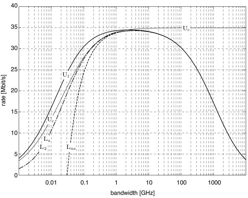
Figure 1: The upper bounds $\mathrm{U}_{\text{{}c}}(W)$ in (28) and $\mathrm{U}_{\text{{}1}}(W)$ in (29), as well as the lower bound $\mathrm{L}_{2}(W)$ in (50), and the large-bandwidth approximations of $\mathrm{L}_{1}(W)$ in (51) and (52) for $\beta=1$ and a brick-shaped scattering function with spread $\Delta_{\operatorname{\mathbb{H}}}=10^{-5}$.

We next evaluate the bounds found in the previous section for the following set of practically relevant system parameters:

• Brick-shaped scattering function with maximum delay $\tau_{0}=0.5\,\mathrm{\text{\textmu}s}$, maximum Doppler shift $\nu_{0}=5\,\mathrm{Hz}$, and corresponding spread $\Delta_{\operatorname{\mathbb{H}}}=4\tau_{0}\nu_{0}=10^{-5}$.

• Grid parameters $T=0.35\,\mathrm{ms}$ and $F=3.53\,\mathrm{kHz}$, so that $TF\approx 1.25$ and $T/F=\tau_{0}/\nu_{0}$, as suggested by the design rule (13).

• Receive power normalized with respect to the noise spectral density

  $$\frac{P}{1\,\mathrm{W}/\,\mathrm{Hz}}=2.42\cdot 10^{7}\sec^{-1}.$$

These parameter values are representative for several different types of systems. For example:

1. An IEEE 802.11a system with transmit power of 200 mW, pathloss of 118$\,\mathrm{dB}$, and receiver noise figure [66] of 5$\,\mathrm{dB}$; the pathloss is rather pessimistic for typical indoor link distances and includes the attenuation of the signal, e.g., by a concrete wall.

2. A UWB system with transmit power of 0.5 mW, pathloss of 77$\,\mathrm{dB}$, and receiver noise figure of 20$\,\mathrm{dB}$.

Fig. 1 shows the upper bounds $\mathrm{U}_{\text{{}c}}(W)$ in (28) and $\mathrm{U}_{\text{{}1}}(W)$ in (29), as well as the lower bound $\mathrm{L}_{2}(W)$ in (50), and the large-bandwidth approximations $\mathrm{L}_{\text{{}a}}(W)$ in (51) and $\mathrm{L}_{\text{{}aa}}(W)$ in (52), all for $\beta=1$.

As brick-shaped scattering functions are flat in the Doppler domain, i.e., they satisfy the condition in (49), it follows from Lemma 3 that the difference between $\mathrm{L}_{\text{{}a}}(W)$ and the lower bound $\mathrm{L}_{2}(W)$ in (50) vanishes as $W\to\infty$. For our choice of parameters, this difference is so small even for finite bandwidth that the curves for $\mathrm{L}_{\text{{}a}}(W)$ and the lower bound $\mathrm{L}_{2}(W)$ cannot be distinguished in Fig. 1. As $\mathrm{L}_{2}(W)\leq\mathrm{L}_{1}(W)\leq\mathrm{L}_{\text{{}a}}(W)$, the lower bound $\mathrm{L}_{1}(W)$ is fully characterized as well.

The upper bound $\mathrm{U}_{\text{{}1}}(W)$ and the lower bound $\mathrm{L}_{1}(W)$ take on their maximum at a large but finite bandwidth; beyond this critical bandwidth, additional bandwidth is detrimental and the capacity approaches zero as bandwidth increases further. In particular, we can see from Fig. 1 that many current wireless systems operate well below the critical bandwidth. It can furthermore be verified numerically that the critical bandwidth increases with decreasing spread, consistent with our analysis in Section III-B3. We also observed that the gap between upper and lower bounds increases with increasing $\beta$.

For bandwidths smaller than the critical bandwidth, $\mathrm{L}_{1}(W)$ comes quite close to the coherent upper bound $\mathrm{U}_{\text{{}c}}(W)$; this seems to validate, at least for the setting considered, the standard receiver design principle to first estimate the channel, and then use the resulting estimates as if they were perfect.

The approximate lower bound $\mathrm{L}_{\text{{}aa}}(W)$ in (52) is accurate for bandwidths above the critical bandwidth and very loose otherwise. Furthermore, $\mathrm{U}_{\text{{}1}}(W)$ and $\mathrm{L}_{\text{{}aa}}(W)$ seem to fully characterize $C(W)$ in the large-bandwidth regime. We will make this statement precise in the next section, where we relate $\mathrm{U}_{\text{{}1}}(W)$ and $\mathrm{L}_{1}(W)$ to the first-order Taylor series expansion of $C(W)$ around the point $1/W=0$.

III-E Capacity in the Infinite-Bandwidth Limit

The plots in Fig. 1 of the upper bound $\mathrm{U}_{\text{{}1}}(W)$ and the lower bound $\mathrm{L}_{1}(W)$ seem to coincide for large bandwidth, yet it is not clear a priori if the two bounds allow to characterize capacity in the limit for $W\to\infty$. To address this question, we next investigate if both bounds have the same first-order Taylor series expansion in $1/W$ around the point $1/W=0$.

Because the upper bound $\mathrm{U}_{\text{{}1}}(W)$ in (29) takes on two different forms, depending on the value of the parameter $\alpha(W)$ in (29b), its first-order Taylor series is somewhat tedious to derive. We state the result in the following lemma and provide the derivation in Appendix E.

Lemma 4

Let

$$\kappa_{\operatorname{\mathbb{H}}} =\iint_{\nu\>\tau}C_{\operatorname{\mathbb{H}}}^{2}(\nu,\tau)d\tau d\nu.$$ (53)

Then, the upper bound (29) in Theorem 1 admits the following first-order Taylor series expansion around the point $1/W=0$:

$$\mathrm{U}_{\text{{}1}}(W) =\frac{c}{W}+\operatorname{\mathit{o}}\mathopen{}\left(\frac{1}{W}\right)$$ (54a)

where

$$c=\lim_{W\to\infty}W\mathrm{U}_{\text{{}1}}(W) =\begin{cases}\dfrac{P^{2}}{2}\left(\beta\kappa_{\operatorname{\mathbb{H}}}-TF\right),&\quad\text{if }\beta>\dfrac{2TF}{\kappa_{\operatorname{\mathbb{H}}}}\\[8.5359pt] \dfrac{(\beta P\kappa_{\operatorname{\mathbb{H}}})^{2}}{8TF},&\quad\text{if }\beta\leq\dfrac{2TF}{\kappa_{\operatorname{\mathbb{H}}}}.\end{cases}$$ (54b)

We show in Appendix F that the corresponding Taylor series expansion of the lower bound $\mathrm{L}_{1}(W)$ in (41) does not have the same first-order term $c$. This result is formalized in the following lemma.

Lemma 5

The lower bound (41) in Theorem 2 admits the following first-order Taylor series expansion around the point $1/W=0$:

$$\mathrm{L}_{1}(W) =\frac{\underline{c}}{W}+\operatorname{\mathit{o}}\mathopen{}\left(\frac{1}{W}\right)$$ (55a)

where

$$\underline{c}=\lim_{W\to\infty}W\mathrm{L}_{1}(W) =\beta P^{2}\left(\frac{\kappa_{\operatorname{\mathbb{H}}}}{2}-TF\right).$$ (55b)

As $c$ in (54b) and $\underline{c}$ in (55b) are different, the two bounds $\mathrm{U}_{\text{{}1}}(W)$ and $\mathrm{L}_{1}(W)$ do not fully characterize $C(W)$ in the wideband limit. In the next theorem, we show, however, that the first-order Taylor series of $\mathrm{U}_{\text{{}1}}(W)$ in Lemma 4 indeed correctly characterizes $C(W)$ for $W\to\infty$.

Theorem 6

Consider an underspread Rayleigh-fading channel with scattering function $C_{\operatorname{\mathbb{H}}}(\nu,\tau)$. Assume that the channel input $\mathbf{x}$ satisfies the average-power constraint $\operatorname{\mathbb{E}}\mathopen{}\left[\lVert\mathbf{x}\rVert^{2}\right]\leq KP\,T$ and the peak constraint $\left\lvert x[k,n]\right\rvert^{2}\leq\beta PT/N$ w.p.1. The capacity $C(W)$ of this channel has a first-order Taylor series expansion around the point $1/W=0$ equal to the first-order Taylor series expansion in (54).

Proof:

We need a capacity lower bound different from $\mathrm{L}_{1}(W)$ with the same asymptotic behavior for $W\to\infty$ as the upper bound $\mathrm{U}_{\text{{}1}}(W)$. The key element in the derivation of this new lower bound is an extension of the block-constant signaling scheme used in [28] to prove asymptotic capacity results for frequency-flat time-selective channels. In particular, we use input signals with uniformly distributed phase whose magnitude is toggled on and off at random with a prescribed probability; hence, information is encoded jointly in the amplitude and in the phase. In comparison, the signaling scheme used to obtain $\mathrm{L}_{1}(W)$ transmits a signal of constant amplitude in all time-frequency slots. We present the details of the proof in Appendix G. ∎

Similar to the capacity behavior of a discrete-time frequency-flat time-selective channel for vanishing SNR [28], the first-order Taylor series coefficient in (54b) can take on two different forms as a function of the channel parameters. However, the link in (16) between the discretized channel and the WSSUS channel $\operatorname{\mathbb{H}}$ allows us to conclude that $\beta>2TF/\kappa_{\operatorname{\mathbb{H}}}$ and thus $c=P^{2}(\beta\kappa_{\operatorname{\mathbb{H}}}-TF)/2$ for virtually all channels of practical interest. In fact, by Jensen’s inequality, $\kappa_{\operatorname{\mathbb{H}}}\geq\Delta_{\operatorname{\mathbb{H}}}^{-1}$ (with equality for brick-shaped scattering functions), so that $2TF\Delta_{\operatorname{\mathbb{H}}}\geq 2TF/\kappa_{\operatorname{\mathbb{H}}}$, and a sufficient condition for $\beta>2TF/\kappa_{\operatorname{\mathbb{H}}}$ is $\beta>2TF\Delta_{\operatorname{\mathbb{H}}}$. For typical values of $TF$ (e.g., $TF\approx 1.25$) and typical values of $\Delta_{\operatorname{\mathbb{H}}}$ (e.g., $\Delta_{\operatorname{\mathbb{H}}}<10^{-2}$), this latter condition is satisfied for any admissible $\beta$.

We state in Lemma 5 that the first-order term $\underline{c}$ in the Taylor series expansion of the lower bound $\mathrm{L}_{1}(W)$ does not match the corresponding term $c$ of the Taylor series expansion of capacity, not even for realistic channel parameters as just discussed. Yet, the plots of the upper bound $\mathrm{U}_{\text{{}1}}(W)$ and the lower bound $\mathrm{L}_{1}(W)$ in Fig. 1 seem to coincide at large bandwidth. This observation is not surprising as the ratio

$$\underline{c}/c=\frac{\beta(\kappa_{\operatorname{\mathbb{H}}}/2-TF)}{(1/2)(\kappa_{\operatorname{\mathbb{H}}}\beta-TF)}$$

approaches $1$ for $\beta$ and $TF$ fixed as $\kappa_{\operatorname{\mathbb{H}}}$ grows large. For example, we have $\underline{c}/c=0.998$ for the same parameters we used for the numerical evaluation in Section III-D, i.e., $\Delta_{\operatorname{\mathbb{H}}}=10^{-3}$, $\beta=1$, and $TF=1.25$.

IV Infinite-Bandwidth Capacity under a Peak Constraint in Time

So far we considered a peak constraint in time and frequency; we now analyze the case when the input signal is subject to a peak constraint in time only, according to (23). The average-power constraint $\operatorname{\mathbb{E}}\mathopen{}\left[\lVert\mathbf{x}\rVert^{2}\right]\leq KP\,T$ remains in force. In addition, we focus on the infinite-bandwidth limit. By means of a capacity lower bound that is explicit in the channel’s scattering function, we show that the phenomenon of vanishing capacity in the wideband limit can be eliminated if we allow the transmit signal to be peaky in frequency. Furthermore, using the same approach as in the proof of Theorem 1, we obtain an upper bound on the infinite-bandwidth capacity that, for $F=1/(2\tau_{0})$, differs from the corresponding lower bound only by a Jensen penalty term. The two bounds coincide for brick-shaped scattering functions when $F=1/(2\tau_{0})$.

The infinite-bandwidth capacity of the channel (11) is defined as

$$C_{\infty}=\lim_{N\to\infty}\lim_{K\to\infty}\sup_{\mathcal{S}}\frac{1}{KT}I(\mathbf{y};\mathbf{x}),$$ (56)

where the supremum is taken over the set $\mathcal{S}$ of all input distributions that satisfy the peak constraint (23) and the constraint $\operatorname{\mathbb{E}}\mathopen{}\left[\lVert\mathbf{x}\rVert^{2}\right]\leq KPT$ on the average power.

IV-A Lower Bound

We obtain a lower bound on $C_{\infty}$ by evaluating the mutual information in (56) for a specific signaling scheme. As signaling scheme, we consider a generalization in the channel’s eigenspace of the on-off FSK scheme proposed in [67]. The resulting lower bound is given in the following theorem.

Theorem 7

Consider an underspread Rayleigh-fading channel with scattering function $C_{\operatorname{\mathbb{H}}}(\nu,\tau)$; assume that the channel input $\mathbf{x}$ satisfies the average-power constraint $\operatorname{\mathbb{E}}\mathopen{}\left[\lVert\mathbf{x}\rVert^{2}\right]\leq KP\,T$ and the peak constraint $\sum_{n=0}^{N-1}\left\lvert x[k,n]\right\rvert^{2}\leq{\beta PT}$ w.p.1. The infinite-bandwidth capacity of this channel is lower-bounded as $C_{\infty}\geq\mathrm{L}_{\infty}$, where

$$\mathrm{L}_{\infty} =P-\frac{1}{\beta}\int_{\nu}\log\mathopen{}\left(1+\beta Pq_{\operatorname{\mathbb{H}}}(\nu)\right)d\nu$$ (57)

and $q_{\operatorname{\mathbb{H}}}(\nu)=\int_{\tau}C_{\operatorname{\mathbb{H}}}(\nu,\tau)d\tau$ denotes the power-Doppler profile of the channel.

Proof:

See Appendix H. ∎

For $\beta=1$, the lower bound in (57) coincides with Viterbi’s result on the rates achievable on an AWGN channel with complex Gaussian input signals with spectral density $q_{\operatorname{\mathbb{H}}}(\nu)$, modulated by FSK tones [23, Eq. (39)]. Viterbi’s setup is relevant for our analysis, because, for a WSSUS channel with power-Doppler profile $q_{\operatorname{\mathbb{H}}}(\nu)$, the output signal that corresponds to an FSK tone can be well-approximated by Viterbi’s transmit signal whenever the observation interval at the receiver is large and the maximum delay $\tau_{0}$ of the channel is much smaller than the observation interval [13, Sec. 8.6]. The proof technique used to obtain Theorem 7 is, however, conceptually different from that in [23]. On the basis of the interpretation of Viterbi’s signaling scheme provided above, we can summarize the proof technique in [23] as follows: first, a signaling scheme is chosen, namely FSK, for transmission over a WSSUS channel; then, the resulting stochastic process at the channel output is discretized by means of a Karhunen-Loève decomposition; finally, the result on the achievable rates in [23, Eq. (39)] follows from an error exponent analysis of the discretized stochastic process and from [13, Lemma 8.5.3]—Szegö’s theorem on the asymptotic eigenvalue distribution of self-adjoint Toeplitz operators.

To prove Theorem 7, on the other hand, we first discretize the WSSUS underspread channel; the rate achievable for a specific signaling scheme, which resembles FSK, yields then the infinite-bandwidth capacity lower bound (57). The main tool used in the proof of Theorem 7 is a property of the information divergence of FSK constellations, first presented by Butman & Klass [36].

For $\beta\to\infty$, i.e., when the input signal is subject only to an average-power constraint, $\mathrm{L}_{\infty}$ in (57) approaches the infinite-bandwidth capacity of an AWGN channel with the same receive power, as previously demonstrated by Gallager [13]. The signaling scheme used in the proof of Theorem 7 is, however, not the only scheme that approaches this limit when no peak constraints are imposed on the input signal. In [15] we presented another signaling scheme, namely, TF pulse position modulation, which exhibits the same behavior. The proof of [15, Th. 1] is similar to the proof of Theorem 7 in Appendix H.

IV-B Upper Bound

In Theorem 8 below we present an upper bound on $C_{\infty}$ and identify a class of scattering functions for which this upper bound and the lower bound (57) coincide if $F=1/(2\tau_{0})$. Differently, from the lower bound, which can be obtained both by Viterbi’s approach and through our approach, the upper bound presented below is heavily built on the discretization of the continuous-time WSSUS underspread channel presented in Section II-B1.

Theorem 8

Consider an underspread Rayleigh-fading channel with scattering function $C_{\operatorname{\mathbb{H}}}(\nu,\tau)$; assume that the channel input $\mathbf{x}$ satisfies the average-power constraint $\operatorname{\mathbb{E}}\mathopen{}\left[\lVert\mathbf{x}\rVert^{2}\right]\leq KP\,T$ and the peak constraint $\sum_{n=0}^{N-1}\left\lvert x[k,n]\right\rvert^{2}\leq{\beta PT}$ w.p.1. The infinite-bandwidth capacity of this channel is upper-bounded as $C_{\infty}\leq\mathrm{U}_{\infty}$, where

$$\mathrm{U}_{\infty}=P-\frac{F}{\beta}\iint_{\nu\>\tau}\log\mathopen{}\left(1+\frac{\beta P}{F}C_{\operatorname{\mathbb{H}}}(\nu,\tau)\right)d\tau d\nu.$$ (58)

Proof:

See Appendix J. ∎

As the upper bound (58) is a decreasing function of $F$, and as $F$ has to satisfy the Nyquist condition $F\leq 1/(2\tau_{0})$, the upper bound is minimized when $F=1/(2\tau_{0})$. For this value of $F$, Jensen’s inequality applied to the second term on the RHS of (58) yields:

$$\begin{split}\frac{1}{2\tau_{0}\beta}\iint_{\nu\>\tau}\log\mathopen{}\left(1+2\tau_{0}\beta PC_{\operatorname{\mathbb{H}}}(\nu,\tau)\right)d\tau d\nu&\leq\frac{1}{\beta}\int_{\nu}\log\mathopen{}\left(1+\beta P\!\int_{\tau}\!C_{\operatorname{\mathbb{H}}}(\nu,\tau)d\tau\right)d\nu\\ &=\frac{1}{\beta}\int_{\nu}\log\mathopen{}\left(1+\beta Pq_{\operatorname{\mathbb{H}}}(\nu)\right)d\nu.\end{split}$$ (59)

Hence, for $F=1/(2\tau_{0})$, the upper bound (58) and the lower bound (57) differ only by a Jensen penalty term. It is interesting to observe that the Jensen penalty in (59) is zero whenever the scattering function is flat in the delay domain, i.e., whenever $C_{\operatorname{\mathbb{H}}}(\nu,\tau)$ is of the form

$$C_{\operatorname{\mathbb{H}}}(\nu,\tau)=\frac{1}{2\tau_{0}}q_{\operatorname{\mathbb{H}}}(\nu),\qquad(\nu,\tau)\in[-\nu_{0},\nu_{0}]\times[-\tau_{0},\tau_{0}].$$ (60)

In this case, upper bound and lower bound coincide and the infinite bandwidth capacity $C_{\infty}$ is fully characterized by

$$C_{\infty}=P-\frac{1}{\beta}\int_{\nu}\log\mathopen{}\left(1+\beta Pq_{\operatorname{\mathbb{H}}}(\nu)\right)d\nu.$$ (61)

Expressions similar to (61) were found in [26] for the capacity per unit energy of a discrete-time frequency-flat time-selective channel, and in [24, 25] for the infinite-bandwidth capacity of the continuous-time counterpart of the same channel; in all cases a peak constraint is imposed on the input signals. However, the results in [24, 25, 26] and our results are not directly related, as discussed next.

IV-B1 Comparison with [24, 25]

The continuous-time time-selective frequency-flat channel analyzed in [24, 25] belongs to the class of LFI channels. As explained in Section II-C, the kernel of an LFI channel cannot be diagonalized as was done in Section II-B1 because LFI channels are not of Hilbert-Schmidt type. Hence, the infinite-bandwidth capacity expressions found in [24, 25] cannot be obtained from our upper and lower bounds simply by an appropriate choice of the scattering function $C_{\operatorname{\mathbb{H}}}(\nu,\tau)$ and of the grid parameters $T$ and $F$.

IV-B2 Comparison with [26]

For scattering functions that are flat in the delay domain [see (60)], the discrete correlation function $R_{\operatorname{\mathbb{H}}}[k,n]$ of our channel is given by

$$R_{\operatorname{\mathbb{H}}}[k,n] =\iint_{\nu\>\tau}C_{\operatorname{\mathbb{H}}}(\nu,\tau)e^{j2\pi(kT\nu-nF\tau)}d\tau d\nu$$

$$=\frac{\sin(2\pi nF\tau_{0})}{2\pi nF\tau_{0}}\int_{\nu}q_{\operatorname{\mathbb{H}}}(\nu)e^{j2\pi kT\nu}d\nu.$$

If we replace $F$ by $1/(2\tau_{0})$, we obtain

$$R_{\operatorname{\mathbb{H}}}[k,n]=\delta[n]\int_{\nu}q_{\operatorname{\mathbb{H}}}(\nu)e^{j2\pi kT\nu}d\nu.$$

Hence, for scattering functions that satisfy (60), and for $F=1/(2\tau_{0})$, the discrete channel $h[k,n]$ is uncorrelated in frequency $n$. Consequently, the input-output relation (21) reduces to the input-output relation of $N$ parallel i.i.d. flat fading channels that are selective in time. However, as both the average power constraint and the peak constraint are imposed on the overall channel and not on each parallel channel separately, the infinite-bandwidth capacity (61) does not follow simply from the capacity per unit energy of one of the parallel channels obtained in [26].

V Conclusions

The underspread Gaussian WSSUS channel with a peak constraint on the input signal is a fairly accurate and general model for wireless channels. Despite the model’s mathematical elegance and simplicity, it appears to be difficult to compute the corresponding capacity. To nonetheless study capacity as a function of bandwidth, we have taken a three-step approach: we first approximated the kernel of the continuous-time WSSUS channel by a kernel that can be diagonalized, and obtained an equivalent discretized channel; in a second step, we derived upper and lower bounds on the capacity of this discretized channel, and in a third step we expressed these bounds in terms of the scattering function of the original continuous-time WSSUS channel. In Section II and Appendix A, we partially characterize the approximation error that arises when the original continuous-time underspread WSSUS channel operator is replaced by a normal operator whose eigenfunctions are a Weyl-Heisenberg set. A complete characterization of the approximation error would require to quantify the difference between the null spaces and between the range spaces of the original operator and its approximation. This characterization is a fundamental open problem, even for deterministic operators.

The capacity bounds derived in this paper are explicit in the channel’s scattering function, a quantity that can be obtained from channel measurements. Furthermore, the capacity bounds may serve as an efficient design tool even when the scattering function is not known completely, and the channel is only characterized coarsely by its maximum delay $\tau_{0}$ and maximum Doppler shift $\nu_{0}$. In particular, one can assume that the scattering function is brick-shaped within its support area $[-\nu_{0},\nu_{0}]\times[-\tau_{0},\tau_{0}]$ and evaluate the corresponding bounds. As shown in Section III-B3 a brick-shaped scattering function results in the lowest upper bound for given $\tau_{0}$ and $\nu_{0}$. Furthermore, the bounds are particularly easy to evaluate for brick-shaped scattering functions and result in analytical expressions explicit in the channel spread $\Delta_{\operatorname{\mathbb{H}}}$. Extensions of the capacity bounds for input signals subject to a peak constraint in time and frequency to the case of spatially correlated MIMO channels are provided in [68].

The multivariate discrete-time channel model considered in this paper, $\mathbf{y}[k]=\mathbf{h}[k]\operatorname{\odot}\mathbf{x}[k]+\mathbf{w}[k]$, and the corresponding capacity bounds are also of interest in their own right, without the connection to the underlying WSSUS channel. The individual elements of the vector $\mathbf{h}[k]$ do not necessarily need to be interpreted as discrete frequency slots; for example, the block-fading model with correlation across blocks in [69] can be cast into the form of our multivariate discrete-time model as well.

As our model is a generalization of the time-selective, frequency-flat channel model, it is not surprising that the structure of our bounds for the case of a peak constraint both in time and frequency, and a peak constraint in time only, is similar to the corresponding results in [27, 28] and [24, 25, 26], respectively. The key difference between our proofs and the proofs in [26, 28, 24] is that our derivation of the upper bounds (29) and (58) (see Appendix B and Appendix J, respectively) is based on the relation between mutual information and MMSE described in [35]. Compared to the proof in [26, Sec. VI], our approach has the advantage that it can easily be generalized to multiple dimensions—in our case time and frequency—and provides the new lower bound (73).

Numerical evaluation indicates that our bounds are surprisingly accurate over a large range of bandwidth. For small bandwidth and hence high SNR, however, our bounds are no longer tight, and a refined analysis along the lines of [5, 70] is called for. In the time-selective frequency-flat case, it was shown in [5] that the high-SNR capacity behavior depends heavily on the spectral density of the channel process. In particular, if the spectral density is zero on a set of positive measure, capacity grows logarithmically in SNR, otherwise the growth is slower, and can even be double-logarithmic. For the more general time- and frequency-selective channel considered in this paper, the assumption that the scattering function is compactly supported implies that the matrix-valued spectral density (40) of the multivariate discrete-time process is zero on a set of positive measure whenever $T<1/(2\nu_{0})$. This implies that the capacity of the approximating channel operator grows logarithmically at high SNR [70] whenever the sampling rate in time is strictly larger than the Nyquist rate. The high-SNR behavior of the capacity of the original channel operator might be different, though. In the approximating discrete-time discrete-frequency input-output relation (11), ISI and ICI are neglected [see (12)]. But the high-SNR behavior of a fading channel is heavily influenced by ISI and ICI, as recently shown in [71].

The approximate kernel diagonalization presented in Section II-B1 can be extended to WSSUS channels with non-compactly supported scattering function, as long as the area of the effective support of the scattering function is small [72]. The capacity bounds corresponding to a non-compactly supported scattering function are, however, more difficult to evaluate numerically, because the periodic repetitions of the scattering function in (16) fall inside the integration region.

A challenging open problem is to characterize the capacity behavior of overspread channels, i.e., channels with spread $\Delta_{\operatorname{\mathbb{H}}}>1$. The major difficulty resides in the fact that a set of deterministic eigenfunctions can no longer be used to diagonalize the random kernel of the channel.

Appendix A

A-A Approximate Eigenfunctions and Eigenvalues of the Channel Operator

The construction of the approximating channel operator in Section II-B1 relies on the following two properties of underspread operators:

• Time and frequency shifts of a time- and frequency-localized prototype signal $g(t)$ matched to the channel’s scattering function $C_{\operatorname{\mathbb{H}}}(\nu,\tau)$, are approximate eigenfunctions of $\operatorname{\mathbb{H}}$.

• Samples of the time-varying transfer function $L_{\operatorname{\mathbb{H}}}(t,f)$ are the corresponding approximate eigenvalues.

In this appendix, we make these claims more precise and give bounds on the mean-square approximation error—averaged with respect to the channel’s realizations—for both approximate eigenfunctions and eigenvalues. The results presented in the remainder of this appendix are not novel, as they already appeared elsewhere, sometimes in different form [20, 72, 56, 42]; the goal of this appendix is rather to provide a self-contained exposition.

A-A1 Ambiguity function

The design problem for $g(t)$ can be restated in terms of its ambiguity function $A_{g}(\nu,\tau)$, which is defined as [73]

$$A_{g}(\nu,\tau)=\int_{t}g(t)g^{*}(t-\tau)e^{-j2\pi\nu t}dt.$$

Without loss of generality, we can assume that $g(t)$ is normalized, so that $A_{g}(0,0)=\lVert g\rVert^{2}=1$. For two signals $g(t)$ and $f(t)$, the cross-ambiguity function is defined as

$$A_{g,f}(\nu,\tau)=\int_{t}g(t)f^{*}(t-\tau)e^{-j2\pi\nu t}dt.$$

The following properties of the (cross-) ambiguity function are important in our context:

Property 1

The volume under the so-called ambiguity surface $\left\lvert A_{g}(\nu,\tau)\right\rvert^{2}$ is constant [74]. In particular, if $g(t)$ has unit energy, then

$$\iint_{\nu\>\tau}\left\lvert A_{g}(\nu,\tau)\right\rvert^{2}d\tau d\nu=1.$$

Property 2

The ambiguity surface attains its maximum magnitude at the origin: $\left\lvert A_{g}(\nu,\tau)\right\rvert^{2}\leq\bigl{[}A_{g}(0,0)\bigr{]}^{2}=1$, for all $\nu$ and $\tau$. This property follows from the Cauchy-Schwarz inequality, as shown in [55].

Property 3

The cross-ambiguity function between the two time- and frequency-shifted signals $g_{(\alpha,\beta)}(t)=g(t-\alpha)e^{j2\pi\beta t}$ and $g_{(\alpha^{\prime},\beta^{\prime})}(t)=g(t-\alpha^{\prime})e^{j2\pi\beta^{\prime}t}$ is given by

$$\begin{split}A_{g_{(\alpha,\beta)},g_{(\alpha^{\prime},\beta^{\prime})}}(\nu,\tau)&=\int_{t}g(t-\alpha)e^{j2\pi\beta t}g^{*}(t-\alpha^{\prime}-\tau)e^{-j2\pi\beta^{\prime}(t-\tau)}e^{-j2\pi\nu t}dt\\ &\stackrel{{\scriptstyle(a)}}{{=}}e^{j2\pi\beta^{\prime}\tau}e^{-j2\pi(\nu+\beta^{\prime}-\beta)\alpha}\int_{t^{\prime}}g(t^{\prime})g^{*}(t^{\prime}-(\alpha^{\prime}-\alpha)-\tau)e^{-j2\pi(\nu+\beta^{\prime}-\beta)t^{\prime}}dt^{\prime}\\ &=A_{g}(\nu+\beta^{\prime}-\beta,\tau+\alpha^{\prime}-\alpha)e^{-j2\pi(\nu\alpha-\tau\beta^{\prime})}e^{-j2\pi(\beta^{\prime}-\beta)\alpha}\end{split}$$ (62)

where (a) follows from the change of variables $t^{\prime}=t-\alpha$. As a direct consequence of (62), we have

$$A_{g_{(\alpha,\beta)}}(\nu,\tau)=A_{g}(\nu,\tau)e^{-j2\pi(\nu\alpha-\tau\beta)}.$$ (63)

Property 4

Let the unit-energy signal $g(t)$ have Fourier transform $G(f)$, and denote by $T_{0}$ and $F_{0}$, defined as

$$T_{0}^{2}=\int_{t}t^{2}\left\lvert g(t)\right\rvert^{2}dt,\quad F_{0}^{2}=\int_{f}f^{2}\left\lvert G(f)\right\rvert^{2}df,$$ (64)

the effective duration and the effective bandwidth of $g(t)$. Then $T_{0}^{2}$ and $F_{0}^{2}$ are proportional to the second-order derivatives of $A_{g}(\nu,\tau)$ at the point $(\nu,\tau)=(0,0)$ [74]

$$\left.\frac{\partial^{2}A_{g}(\nu,\tau)}{\partial\nu^{2}}\right|_{(\nu,\tau)=(0,0)} =-4\pi^{2}T_{0}^{2}$$

$$\left.\frac{\partial^{2}A_{g}(\nu,\tau)}{\partial\tau^{2}}\right|_{(\nu,\tau)=(0,0)} =-4\pi^{2}F_{0}^{2}.$$

Property 5

For the channel operator $\operatorname{\mathbb{H}}$ in Section II-A,

$$\langle\operatorname{\mathbb{H}}g,f\rangle \stackrel{{\scriptstyle(a)}}{{=}}\iiint_{t\,\,\tau\,\,\nu}S_{\operatorname{\mathbb{H}}}(\nu,\tau)g(t-\tau)e^{j2\pi t\nu}f^{*}(t)d\tau d\nu dt$$

$$=\iint_{\nu\>\tau}S_{\operatorname{\mathbb{H}}}(\nu,\tau)\Biggl{[}\int_{t}f(t)g^{*}(t-\tau)e^{-j2\pi t\nu}dt\Biggr{]}^{*}d\tau d\nu$$

$$=\iint_{\nu\>\tau}S_{\operatorname{\mathbb{H}}}(\nu,\tau)A^{*}_{f,g}(\nu,\tau)d\tau d\nu=\langle S_{\operatorname{\mathbb{H}}},A_{f,g}\rangle$$

where in (a) we used (5).

Properties 1 and 2, which constitute the radar uncertainty principle, imply that it is not possible to find a signal $g(t)$ with a corresponding ambiguity function $A_{g}(\nu,\tau)$ that is arbitrarily well concentrated in $\nu$ and $\tau$ [74]. The radar uncertainty principle is a manifestation of the classical Heisenberg uncertainty principle, which states that the effective duration $T_{0}$ and the effective bandwidth $F_{0}$ [both defined in (64)] of any signal in $\mathcal{L}^{2}$ satisfy $T_{0}F_{0}\geq 1/(4\pi)$ [55, Th. 2.2.1]. In fact, when $g(t)$ has effective duration $T_{0}$, and effective bandwidth $F_{0}$, the corresponding ambiguity function $A_{g}(\nu,\tau)$ is highly concentrated on a rectangle of area $4T_{0}F_{0}$; but this area cannot be made arbitrarily small.

A-A2 Approximate Eigenfunctions

Lemma 9 (​ [20, Ch. 4.6.1])

Let $\operatorname{\mathbb{H}}$ be a WSSUS channel with scattering function $C_{\operatorname{\mathbb{H}}}(\nu,\tau)$. Then, for any unit-energy signal $g(t)$, the mean-square approximation error incurred by assuming that $g(t)$ is an eigenfunction of $\operatorname{\mathbb{H}}$ is given by

$$\epsilon_{1}=\operatorname{\mathbb{E}}\mathopen{}\left[\lVert\langle\operatorname{\mathbb{H}}g,g\rangle g-\operatorname{\mathbb{H}}g\rVert^{2}\right]=\iint_{\nu\>\tau}C_{\operatorname{\mathbb{H}}}(\nu,\tau)\left(1-\left\lvert A_{g}(\nu,\tau)\right\rvert^{2}\right)d\tau d\nu.$$ (65)

Proof:

We decompose $\epsilon_{1}$ as follows:

$$\begin{split}\operatorname{\mathbb{E}}\mathopen{}\left[\lVert\langle\operatorname{\mathbb{H}}g,g\rangle g-\operatorname{\mathbb{H}}g\rVert^{2}\right]&=\operatorname{\mathbb{E}}\mathopen{}\left[\lVert\langle\operatorname{\mathbb{H}}g,g\rangle g\rVert^{2}\right]+\operatorname{\mathbb{E}}\mathopen{}\left[\lVert\operatorname{\mathbb{H}}g\rVert^{2}\right]-2\operatorname{\mathbb{E}}\mathopen{}\left[\left\lvert\langle\operatorname{\mathbb{H}}g,g\rangle\right\rvert^{2}\right]\\ &=\operatorname{\mathbb{E}}\mathopen{}\left[\lVert\operatorname{\mathbb{H}}g\rVert^{2}\right]-\operatorname{\mathbb{E}}\mathopen{}\left[\left\lvert\langle\operatorname{\mathbb{H}}g,g\rangle\right\rvert^{2}\right].\end{split}$$ (66)

Here, the last steps follows because $g(t)$ has unit energy by assumption. We now compute the two terms in (66) separately. The first term is equal to

$$\begin{split}\operatorname{\mathbb{E}}\mathopen{}\left[\lVert\operatorname{\mathbb{H}}g\rVert^{2}\right]&\stackrel{{\scriptstyle(a)}}{{=}}\operatorname{\mathbb{E}}\mathopen{}\left[\int_{t}\left\lvert\iint_{\nu\>\tau}S_{\operatorname{\mathbb{H}}}(\nu,\tau)g(t-\tau)e^{j2\pi t\nu}d\tau d\nu\right\rvert^{2}dt\right]\\ &\stackrel{{\scriptstyle(b)}}{{=}}\iint_{\nu\>\tau}C_{\operatorname{\mathbb{H}}}(\nu,\tau)\int_{t}g(t-\tau)g^{*}(t-\tau)dtd\tau d\nu\\ &\stackrel{{\scriptstyle(c)}}{{=}}\iint_{\nu\>\tau}C_{\operatorname{\mathbb{H}}}(\nu,\tau)d\tau d\nu\end{split}$$ (67)

where (a) follows from (5), (b) from the WSSUS property, and (c) from the energy normalization of $g(t)$. For the second term we have

$$\begin{split}\operatorname{\mathbb{E}}\mathopen{}\left[\left\lvert\langle\operatorname{\mathbb{H}}g,g\rangle\right\rvert^{2}\right]&\stackrel{{\scriptstyle(a)}}{{=}}\operatorname{\mathbb{E}}\mathopen{}\left[\left\lvert\langle S_{\operatorname{\mathbb{H}}},A_{g}\rangle\right\rvert^{2}\right]=\operatorname{\mathbb{E}}\mathopen{}\left[\left\lvert\iint_{\nu\>\tau}S_{\operatorname{\mathbb{H}}}(\nu,\tau)A^{*}_{g}(\nu,\tau)d\tau d\nu\right\rvert^{2}\right]\\ &\stackrel{{\scriptstyle(b)}}{{=}}\iint_{\nu\>\tau}C_{\operatorname{\mathbb{H}}}(\nu,\tau)\left\lvert A_{g}(\nu,\tau)\right\rvert^{2}d\tau d\nu\end{split}$$ (68)

where (a) follows from Property 5 and (b) follows from the WSSUS property. To conclude the proof, we substitute (67) and (68) in (66). ∎

The error $\epsilon_{1}$ in (65) is minimized if $g(t)$ is chosen so that $A_{g}(\nu,\tau)\approx A_{g}(0,0)=1$ over the support of the scattering function. If the channel is highly underspread, we can replace $A_{g}(\nu,\tau)$ on the RHS of (65) with its second-order Taylor series expansion around the point $(\nu,\tau)=(0,0)$; Property 4 now shows that good time and frequency localization of $g(t)$ is necessary for $\epsilon_{1}$ to be small. If $g(t)$ is taken to be real and even, the second-order Taylor series expansion of $A_{g}(\nu,\tau)$ around the point $(\nu,\tau)=(0,0)$ takes on a particularly simple form because the first-order term is zero, and we can approximate $A_{g}(\nu,\tau)$ around $(0,0)$ as follows [74]:

$$A_{g}(\nu,\tau)\approx 1-2\pi\left[T_{0}^{2}\nu^{2}+F_{0}^{2}\tau^{2}-j\nu\tau/(4\pi)\right].$$

Hence, when $g(t)$ is real and even, good time and frequency localization of $g(t)$ is also sufficient for $\epsilon_{1}$ to be small.

A-A3 Approximate Eigenvalues

Lemma 10 (​[72, 42])

Let $\operatorname{\mathbb{H}}$ be a WSSUS channel with time-varying transfer function $L_{\operatorname{\mathbb{H}}}(t,f)$ and scattering function $C_{\operatorname{\mathbb{H}}}(\nu,\tau)$. Then, for any unit-energy signal $g_{(\alpha,\beta)}(t)=g(t-\alpha)e^{j2\pi\beta t}$, the mean-square approximation error incurred by assuming that $L_{\operatorname{\mathbb{H}}}(\alpha,\beta)$ is an eigenvalue of $\operatorname{\mathbb{H}}$ associated to $g_{(\alpha,\beta)}(t)$ is given by

$$\epsilon_{2} =\operatorname{\mathbb{E}}\mathopen{}\left[\left\lvert\langle\operatorname{\mathbb{H}}g_{(\alpha,\beta)},g_{(\alpha,\beta)}\rangle-L_{\operatorname{\mathbb{H}}}(\alpha,\beta)\right\rvert^{2}\right]=\iint_{\nu\>\tau}C_{\operatorname{\mathbb{H}}}(\nu,\tau)\left\lvert 1-A_{g}(\nu,\tau)\right\rvert^{2}d\tau d\nu.$$

Proof:

We use Property 5 and the Fourier transform relation (4) to write $\epsilon_{2}$ as

$$\begin{split}\epsilon_{2}&=\operatorname{\mathbb{E}}\mathopen{}\left[\left\lvert\iint_{\nu\>\tau}S_{\operatorname{\mathbb{H}}}(\nu,\tau)\left[A^{*}_{g_{(\alpha,\beta)}}(\nu,\tau)-e^{j2\pi(\nu\alpha-\tau\beta)}\right]d\tau d\nu\right\rvert^{2}\right]\\ &\stackrel{{\scriptstyle(a)}}{{=}}\operatorname{\mathbb{E}}\mathopen{}\left[\left\lvert\iint_{\nu\>\tau}S_{\operatorname{\mathbb{H}}}(\nu,\tau)e^{j2\pi(\nu\alpha-\tau\beta)}\left[A^{*}_{g}(\nu,\tau)-1\right]d\tau d\nu\right\rvert^{2}\right]\\ &\stackrel{{\scriptstyle(b)}}{{=}}\iint_{\nu\>\tau}C_{\operatorname{\mathbb{H}}}(\nu,\tau)\left\lvert 1-A_{g}(\nu,\tau)\right\rvert^{2}d\tau d\nu.\end{split}$$ (69)

Here, (a) follows from (63) and (b) is a consequence of the WSSUS property. ∎

Similarly to what was stated for $\epsilon_{1}$ in the previous section, also in this case good time and frequency localization of $g(t)$ leads to small mean-square error $\epsilon_{2}$ if the channel is underspread.

A-B OFDM Pulse Design for Minimum ISI and ICI

In Section II-B3 we introduced the concept of a PS-OFDM system that uses an orthonormal Weyl-Heisenberg transmission set $\{g_{k,n}(t)\}$, where $g_{k,n}(t)=g(t-kT)e^{j2\pi nFt}$, and provided the criterion (13) for the choice of the grid parameters $T$ and $F$ to jointly minimize ISI and ICI. In this section, we detail the derivation that leads to (13). Let $r(t)=(\operatorname{\mathbb{H}}x)(t)$ denote the noise-free channel output when the channel input $x(t)$ is a PS-OFDM signal given by

$$x(t)=\sum_{k=-\infty}^{\infty}\sum_{n=-\infty}^{\infty}x[k,n]g_{k,n}(t).$$

For mathematical convenience, we consider the case of an infinite time and frequency horizon, and assume that the input symbols $\{x[k,n]\}$ are i.i.d., with zero mean and $\operatorname{\mathbb{E}}\mathopen{}\left[\left\lvert x[k,n]\right\rvert^{2}\right]\leq 1$, $\forall k,n$.

We want to quantify the mean-square error incurred by assuming that the projection of the received signal $r(t)$ onto the function $g_{k,n}(t)$ equals $x[k,n]L_{\operatorname{\mathbb{H}}}(kT,nF)$, i.e., the error

$$\epsilon_{3}=\operatorname{\mathbb{E}}\mathopen{}\left[\left\lvert\langle r,g_{k,n}\rangle-x[k,n]L_{\operatorname{\mathbb{H}}}(kT,nF)\right\rvert^{2}\right]$$

where the expectation is over the channel realizations and the input symbols. We bound $\epsilon_{3}$ as follows:

$$\begin{split}\epsilon_{3}&=\operatorname{\mathbb{E}}\Bigl{[}\bigl{\lvert}\langle r,g_{k,n}\rangle-x[k,n]\langle\operatorname{\mathbb{H}}g_{k,n},g_{k,n}\rangle\\ &\hphantom{\leq\operatorname{\mathbb{E}}\Bigl{[}\lvert\langle r,g_{k,n}\rangle}+x[k,n]\bigl{(}\langle\operatorname{\mathbb{H}}g_{k,n},g_{k,n}\rangle-L_{\operatorname{\mathbb{H}}}(kT,nF)\bigr{)}\bigr{\rvert}^{2}\Bigr{]}\\ &\stackrel{{\scriptstyle(a)}}{{\leq}}2\underbrace{\operatorname{\mathbb{E}}\mathopen{}\left[\left\lvert\langle r,g_{k,n}\rangle-x[k,n]\langle\operatorname{\mathbb{H}}g_{k,n},g_{k,n}\rangle\right\rvert^{2}\right]}_{\epsilon_{4}}\\ &\hphantom{\leq\operatorname{\mathbb{E}}\Bigl{[}\lvert\langle r,g_{k,n}\rangle}+2\operatorname{\mathbb{E}}\mathopen{}\left[\left\lvert x[k,n]\bigl{(}\langle\operatorname{\mathbb{H}}g_{k,n},g_{k,n}\rangle-L_{\operatorname{\mathbb{H}}}(kT,nF)\bigr{)}\right\rvert^{2}\right]\\ &=2\epsilon_{4}+2\operatorname{\mathbb{E}}\mathopen{}\left[\left\lvert x[k,n]\right\rvert^{2}\right]\underbrace{\operatorname{\mathbb{E}}\mathopen{}\left[\bigl{\lvert}\langle\operatorname{\mathbb{H}}g_{k,n},g_{k,n}\rangle-L_{\operatorname{\mathbb{H}}}(kT,nF)\bigr{\rvert}^{2}\right]}_{\epsilon_{2}}\\ &\leq 2\epsilon_{4}+2\epsilon_{2}\end{split}$$

where (a) holds because for any two complex numbers $u$ and $v$ we have that $\left\lvert u+v\right\rvert^{2}\leq 2\left\lvert u\right\rvert^{2}+2\left\lvert v\right\rvert^{2}$. The error $\epsilon_{2}$ is the same as the one computed in Lemma 10. The error $\epsilon_{4}$ results from neglecting ISI and ICI and can be bounded as follows:

$$\begin{split}\epsilon_{4}=&\operatorname{\mathbb{E}}\mathopen{}\left[\left\lvert\langle r,g_{k,n}\rangle\right\rvert^{2}\right]+\operatorname{\mathbb{E}}\mathopen{}\left[\left\lvert x[k,n]\right\rvert^{2}\right]\operatorname{\mathbb{E}}\mathopen{}\left[\left\lvert\langle\operatorname{\mathbb{H}}g_{k,n},g_{k,n}\rangle\right\rvert^{2}\right]\\ &-2\Re\mathopen{}\left\{\operatorname{\mathbb{E}}\mathopen{}\left[x^{*}[k,n]\langle r,g_{k,n}\rangle\langle\operatorname{\mathbb{H}}g_{k,n},g_{k,n}\rangle^{*}\right]\right\}\\ \stackrel{{\scriptstyle(a)}}{{=}}&\mathop{\sum_{k^{\prime}=-\infty}^{\infty}\sum_{n^{\prime}=-\infty}^{\infty}}_{(k^{\prime},n^{\prime})\neq(k,n)}\operatorname{\mathbb{E}}\mathopen{}\left[\left\lvert x[k^{\prime},n^{\prime}]\right\rvert^{2}\right]\operatorname{\mathbb{E}}\mathopen{}\left[\left\lvert\langle\operatorname{\mathbb{H}}g_{k^{\prime},n^{\prime}},g_{k,n}\rangle\right\rvert^{2}\right]\\ \stackrel{{\scriptstyle(b)}}{{\leq}}&\mathop{\sum_{k^{\prime}=-\infty}^{\infty}\sum_{n^{\prime}=-\infty}^{\infty}}_{(k^{\prime},n^{\prime})\neq(k,n)}\operatorname{\mathbb{E}}\mathopen{}\left[\left\lvert\langle\operatorname{\mathbb{H}}g_{k^{\prime},n^{\prime}},g_{k,n}\rangle\right\rvert^{2}\right]\end{split}$$ (70)

where (a) follows because the $x[k,n]$ are i.i.d. and zero mean, and (b) because $\operatorname{\mathbb{E}}\mathopen{}\left[\left\lvert x[k,n]\right\rvert^{2}\right]\leq 1$. We now provide an expression for $\operatorname{\mathbb{E}}\mathopen{}\left[\left\lvert\langle\operatorname{\mathbb{H}}g_{k^{\prime},n^{\prime}},g_{k,n}\rangle\right\rvert^{2}\right]$ that is explicit in the channel’s scattering function:

$$\begin{split}\operatorname{\mathbb{E}}\mathopen{}\left[\left\lvert\langle\operatorname{\mathbb{H}}g_{k^{\prime},n^{\prime}},g_{k,n}\rangle\right\rvert^{2}\right]&\stackrel{{\scriptstyle(a)}}{{=}}\operatorname{\mathbb{E}}\mathopen{}\left[\left\lvert\langle S_{\operatorname{\mathbb{H}}},A_{g_{k,n},g_{k^{\prime},n^{\prime}}}\rangle\right\rvert^{2}\right]\\ &\stackrel{{\scriptstyle(b)}}{{=}}\iint_{\nu\>\tau}C_{\operatorname{\mathbb{H}}}(\nu,\tau)\left\lvert A_{g_{k,n},g_{k^{\prime},n^{\prime}}}(\nu,\tau)\right\rvert^{2}d\tau d\nu\\ &\stackrel{{\scriptstyle(c)}}{{=}}\iint_{\nu\>\tau}C_{\operatorname{\mathbb{H}}}(\nu,\tau)\left\lvert A_{g}\mathopen{}\left(\nu+(n^{\prime}-n)F,\tau+(k^{\prime}-k)T\right)\right\rvert^{2}d\tau d\nu\\ &\stackrel{{\scriptstyle}}{{=}}\iint_{\nu\>\tau}C_{\operatorname{\mathbb{H}}}\mathopen{}\left(\nu-(n^{\prime}-n)F,\tau-(k^{\prime}-k)T\right)\left\lvert A_{g}(\nu,\tau)\right\rvert^{2}d\tau d\nu.\end{split}$$ (71)

Here, (a) follows from Property 5, (b) from the WSSUS property, and (c) from Property 3. We finally substitute (71) in (70) and obtain

$$\begin{split}\epsilon_{4}\leq&\mathop{\sum_{k^{\prime}=-\infty}^{\infty}\sum_{n^{\prime}=-\infty}^{\infty}}_{(k^{\prime},n^{\prime})\neq(k,n)}\iint_{\nu\>\tau}C_{\operatorname{\mathbb{H}}}\mathopen{}\left(\nu-(n^{\prime}-n)F,\tau-(k^{\prime}-k)T\right)\left\lvert A_{g}(\nu,\tau)\right\rvert^{2}d\tau d\nu\\ =&\mathop{\sum_{k=-\infty}^{\infty}\sum_{n=-\infty}^{\infty}}_{(k,n)\neq(0,0)}\iint_{\nu\>\tau}C_{\operatorname{\mathbb{H}}}(\nu-nF,\tau-kT)\left\lvert A_{g}(\nu,\tau)\right\rvert^{2}d\tau d\nu.\end{split}$$ (72)

This error is small if the ambiguity surface $\left\lvert A_{g}(\nu,\tau)\right\rvert^{2}$ of $g(t)$ takes on small values on the periodically repeated rectangles $[-\nu_{0}+nF,\nu_{0}+nF]\times[-\tau_{0}+kT,\tau_{0}+kT]$, except for the dashed rectangle centered at the origin (see Fig. 2).

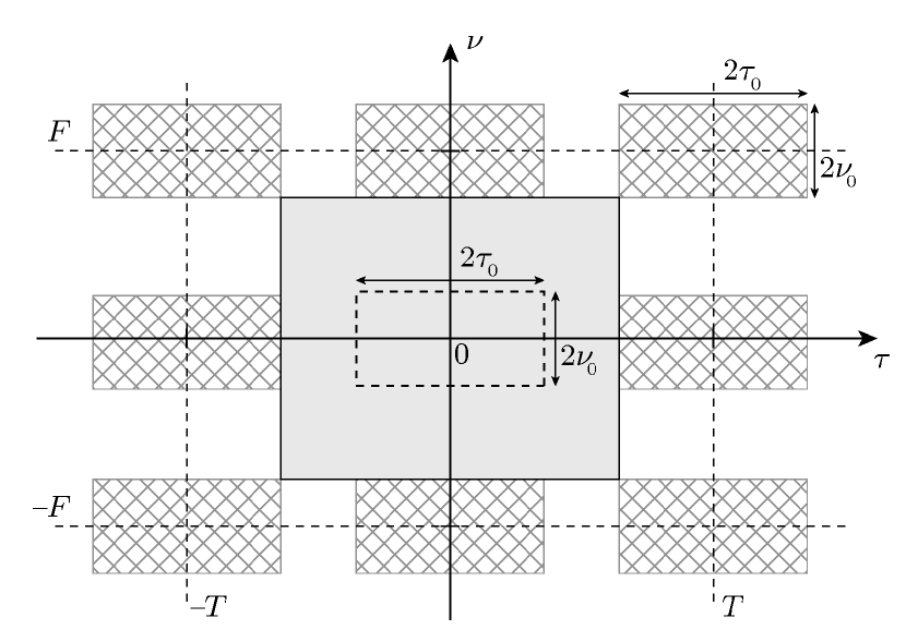
Figure 2: The support set of the periodized scattering function in (72) are the rectangles with crisscross pattern, while the area on which the ambiguity function $A_{g}(\nu,\tau)$ should be concentrated to minimize $\epsilon_{4}$ is shaded in grey.

This condition can be satisfied if the channel is highly underspread and if the grid parameters $T$ and $F$ are chosen such that the solid rectangle centered at the origin in Fig. 2 has large enough area to allow $\left\lvert A_{g}(\nu,\tau)\right\rvert^{2}$ to decay. If $g(t)$ has effective duration $T_{0}$ and effective bandwidth $F_{0}$, the latter condition holds if $T\geq\tau_{0}+T_{0}$, and $F\geq\nu_{0}+F_{0}$. Given a constraint on the product $TF$, good localization of $g(t)$, both in time and frequency, is necessary for the two inequalities above to hold.

The minimization of $\epsilon_{4}$ in (72) over all orthonormal Weyl-Heisenberg sets $\{g_{k,n}(t)\}$ is a difficult task; numerical methods to minimize $\epsilon_{4}$ are described in [58]. The simple rule on how to choose the grid parameters $T$ and $F$ provided in (13) is derived from the following observation: for known $\tau_{0}$ and $\nu_{0}$, and for a fixed product $TF$, the area $4(T-\tau_{0})(F-\nu_{0})$ of the solid rectangle centered at the origin in Fig. 2 is maximized if [20, 56, 58]

$$\frac{T}{F}=\frac{\tau_{0}}{\nu_{0}}.$$

Appendix B

Lemma 11

Let $\{h[k]\}$ be a stationary random process with correlation function

$$r_{h}[k]=\operatorname{\mathbb{E}}\mathopen{}\left[h[k^{\prime}+k]h^{*}[k^{\prime}]\right]$$

and spectral density

$$c_{h}(\theta)=\sum_{k=-\infty}^{\infty}r_{h}[k]e^{-j2\pi k\theta},\quad\left\lvert\theta\right\rvert\leq 1/2.$$

Furthermore, let $\mathbf{h}=\big{[}\begin{matrix}h[0]\,h[1]\,\dots\,h[K-1]\end{matrix}\big{]}\raisebox{0.34444pt}{\vphantom{M}}^{T}$, and denote the $K\times K$ covariance matrix of $\mathbf{h}$ by $\mathbf{R}_{\mathbf{h}}=\operatorname{\mathbb{E}}\mathopen{}\left[\mathbf{h}\mathbf{h}^{H}\right]$. This covariance matrix is Hermitian Toeplitz with entries $\left[\mathbf{R}_{\mathbf{h}}\right]_{i,j}=r_{h}[i-j]$. Then, for any deterministic $K$-dimensional vector $\mathbf{x}$ with binary entries $\{0,1\}$ and for any $\rho>0$, the following inequality holds:

$$\inf_{\mathbf{x}}\frac{1}{\lVert\mathbf{x}\rVert^{2}}\log\det\mathopen{}\left(\mathbf{I}_{K}+\rho(\mathbf{x}\mathbf{x}^{H})\operatorname{\odot}\mathbf{R}_{\mathbf{h}}\right)\geq\int_{-1/2}^{1/2}\log(1+\rho c_{h}(\theta))d\theta.$$ (73)

Furthermore, in the limit $K\to\infty$, the above inequality is satisfied with equality if the entries of $\mathbf{x}$ are all equal to $1$.

Remark 1

The second statement in Lemma 11—that the infimum can be achieved by an all-$1$ vector in the limit for $K\to\infty$—was already proved in [26, Sec. VI.B]. The proof in [26] relies on rather technical set-theoretic arguments, so that it is not easy to see how the structure of the problem—the stationarity of the process $\{h[k]\}$—comes into play. Therefore, it is cumbersome to extend the proof in [26] to accommodate two-dimensional stationary processes as used in this paper. Here, we provide an alternative proof that is significantly shorter, explicitly uses the stationarity property, can be directly generalized to two-dimensional stationary processes (see Corollary 13 below), and yields the new lower bound (73) as an important additional result.

Our proof is based on the relation between mutual information MMSE discovered recently by Guo et al. [35]. In the following lemma, we restate, for convenience, the mutual information-MMSE relation for JPG random vectors

Lemma 12

Let $\mathbf{h}$ be a $K$-dimensional random vector that satisfies $\operatorname{\mathbb{E}}\mathopen{}\left[\lVert\mathbf{h}\rVert^{2}\right]<\infty$, and let $\mathbf{w}$ be a zero-mean JPG vector, $\mathbf{w}\sim\mathcal{CN}(\mathbf{0},\mathbf{I}_{K})$, that is independent of $\mathbf{h}$. Then, for any deterministic $K$-dimensional vector $\mathbf{x}$,

$$\frac{d}{d\gamma}I(\sqrt{\gamma}\mathbf{x}\operatorname{\odot}\mathbf{h}+\mathbf{w};\mathbf{h})=\operatorname{\mathbb{E}}\mathopen{}\left[\lVert\mathbf{x}\operatorname{\odot}\mathbf{h}-\mathbf{x}\operatorname{\odot}\operatorname{\mathbb{E}}\mathopen{}\left[\mathbf{h}\,|\,\sqrt{\gamma}\mathbf{x}\operatorname{\odot}\mathbf{h}+\mathbf{w}\right]\rVert^{2}\right].$$ (74)

The expression on the RHS in (74) is the MMSE obtained when $\mathbf{x}\operatorname{\odot}\mathbf{h}$ is estimated from the noisy observation $\sqrt{\gamma}\mathbf{x}\operatorname{\odot}\mathbf{h}+\mathbf{w}$.

Proof:

We first derive the lower bound (73) and then show achievability in the limit $K\to\infty$ in a second step. To apply Lemma 12, we rewrite the LHS of (73) as

$$\frac{1}{\lVert\mathbf{x}\rVert^{2}}\log\det\mathopen{}\left(\mathbf{I}_{K}+\rho(\mathbf{x}\mathbf{x}^{H})\operatorname{\odot}\mathbf{R}_{\mathbf{h}}\right)=\frac{1}{\lVert\mathbf{x}\rVert^{2}}I(\sqrt{\rho}\mathbf{x}\operatorname{\odot}\mathbf{h}+\mathbf{w};\mathbf{h})$$ (75)

where $\mathbf{w}\sim\mathcal{CN}(\mathbf{0},\mathbf{I}_{K})$ is a JPG vector. Without loss of generality, we assume that the vector $\mathbf{x}$ has exactly $M$ nonzero entries, with corresponding indices in the set $\mathcal{M}$. Then,

$$\begin{split}\frac{1}{\lVert\mathbf{x}\rVert^{2}}I(&\sqrt{\rho}\mathbf{x}\operatorname{\odot}\mathbf{h}+\mathbf{w};\mathbf{h})=\\ &\stackrel{{\scriptstyle(a)}}{{=}}\frac{1}{\lVert\mathbf{x}\rVert^{2}}\int_{0}^{\rho}\operatorname{\mathbb{E}}\mathopen{}\left[\lVert\mathbf{x}\operatorname{\odot}\mathbf{h}-\mathbf{x}\operatorname{\odot}\operatorname{\mathbb{E}}\mathopen{}\left[\mathbf{h}\,|\,\sqrt{\gamma}\mathbf{x}\operatorname{\odot}\mathbf{h}+\mathbf{w}\right]\rVert^{2}\right]d\gamma\\ &\stackrel{{\scriptstyle(b)}}{{=}}\frac{1}{M}\int_{0}^{\rho}\sum_{m\in\mathcal{M}}\operatorname{\mathbb{E}}\mathopen{}\left[\left\lvert h[m]-\operatorname{\mathbb{E}}\mathopen{}\left[h[m]\,|\,\mathopen{}\left\{\sqrt{\gamma}h[k]+w[k]\right\}_{k\in\mathcal{M}}\right]\right\rvert^{2}\right]d\gamma\\ &\stackrel{{\scriptstyle(c)}}{{\geq}}\frac{1}{M}\int_{0}^{\rho}\sum_{m\in\mathcal{M}}\operatorname{\mathbb{E}}\mathopen{}\left[\left\lvert h[m]-\operatorname{\mathbb{E}}\mathopen{}\left[h[m]\,|\,\mathopen{}\left\{\sqrt{\gamma}h[k]+w[k]\right\}_{k=-\infty}^{\infty}\right]\right\rvert^{2}\right]d\gamma\\ &\stackrel{{\scriptstyle(d)}}{{=}}\int_{0}^{\rho}\operatorname{\mathbb{E}}\mathopen{}\left[\left\lvert h[0]-\operatorname{\mathbb{E}}\mathopen{}\left[h[0]\,|\,\mathopen{}\left\{\sqrt{\gamma}h[k]+w[k]\right\}_{k=-\infty}^{\infty}\right]\right\rvert^{2}\right]d\gamma.\end{split}$$ (76)

Here, (a) follows from the relation between mutual information and MMSE in Lemma 12 in the form given in [35, Eq. (47)]. Equality (b) holds because $\mathbf{x}$ has exactly $M$ nonzero entries with corresponding indices in $\mathcal{M}$, and because the components of the observation that contain only noise do not influence the estimation error. The argument underlying inequality (c) is that the MMSE can only decrease if each $h[m]$ is estimated not just from a finite set of noisy observations of the random process $\{h[k]\}$, but also from noisy observations of the process’ infinite past and future. This is the so-called infinite-horizon noncausal MMSE. Finally, we obtain (d) because the process $\{h[k]\}$ is stationary and its infinite horizon noncausal MMSE is, therefore, the same for all indices $m\in\mathcal{M}$ [75, Sec. V.D.1].

The infinite-horizon noncausal MMSE can be expressed in terms of the spectral density of the process $\{h[k]\}$ [75, Eq. (V.D.28)]:

$$\operatorname{\mathbb{E}}\mathopen{}\left[\left\lvert h[0]-\operatorname{\mathbb{E}}\mathopen{}\left[h[0]\,|\,\mathopen{}\left\{\sqrt{\gamma}h[k]+w[k]\right\}_{k=-\infty}^{\infty}\right]\right\rvert^{2}\right]=\int_{-1/2}^{1/2}\frac{c_{h}(\theta)}{1+\gamma c_{h}(\theta)}d\theta.$$ (77)

To obtain the desired inequality (73), we substitute (77) in (76), and (76) in (75), and note that the resulting lower bound does not depend on $\mathbf{x}$. We have therefore established a lower bound on the LHS of (73) as well. We finally integrate over $\gamma$ and get

$$\begin{split}\inf_{\mathbf{x}}\frac{1}{\lVert\mathbf{x}\rVert^{2}}\log\det\mathopen{}\left(\mathbf{I}_{K}+\rho(\mathbf{x}\mathbf{x}^{H})\operatorname{\odot}\mathbf{R}_{\mathbf{h}}\right)&\geq\int_{-1/2}^{1/2}\int_{0}^{\rho}\frac{c_{h}(\theta)}{1+\gamma c_{h}(\theta)}d\gamma d\theta\\ &=\int_{-1/2}^{1/2}\log\bigl{(}1+\rho c_{h}(\theta)\bigr{)}d\theta.\end{split}$$

To prove the second statement in Lemma 11, we choose $\mathbf{x}$ in (75) to be the all-$1$ vector for any dimension $K$, and evaluate the limit $K\to\infty$ of the LHS of (75) by means of Szegö’s theorem on the asymptotic eigenvalue distribution of a Toeplitz matrix [31, 32]:

$$\lim_{K\to\infty}\frac{1}{K}\log\det\mathopen{}\left(\mathbf{I}_{K}+\rho\mathbf{R}_{\mathbf{h}}\right)=\int_{-1/2}^{1/2}\log\bigl{(}1+\rho c_{h}(\theta)\bigr{)}d\theta.$$ (78)

This shows that the lower bound in (73) can indeed be achieved in the limit $K\to\infty$ when $\mathbf{x}$ is the all-$1$ vector. ∎

Our proof allows for a simple generalization of Lemma 11 to two-dimensional stationary processes, which are relevant to the problem considered in this paper. The generalization is stated in the following corollary.

Corollary 13

Let $\{h[k,n]\}$ be a random process that is stationary in $k$ and $n$ with two-dimensional correlation function $r_{h}[k,n]=\operatorname{\mathbb{E}}\mathopen{}\left[h[k+k^{\prime},n+n^{\prime}]h^{*}[k^{\prime},n^{\prime}]\right]$ and two-dimensional spectral density

$$c_{h}(\theta,\varphi)=\sum_{k=-\infty}^{\infty}\sum_{n=-\infty}^{\infty}r_{h}[k,n]e^{-j2\pi(k\theta-n\varphi)},\quad\left\lvert\theta\right\rvert,\left\lvert\varphi\right\rvert\leq 1/2.$$

Furthermore, let $\mathbf{h}[k]=\big{[}\begin{matrix}h[k,0]&h[k,1]&\cdots&h[k,N-1]\end{matrix}\big{]}\raisebox{0.34444pt}{\vphantom{M}}^{T}$, let the $KN$-dimensional stacked vector $\mathbf{h}=\big{[}\begin{matrix}\mathbf{h}^{T}[0]\,\mathbf{h}^{T}[1]\,\dots\,\mathbf{h}^{T}[K-1]\end{matrix}\big{]}\raisebox{0.34444pt}{\vphantom{M}}^{T}$, and denote the $KN\times KN$ covariance matrix of $\mathbf{h}$ by $\mathbf{R}_{\mathbf{h}}=\operatorname{\mathbb{E}}\mathopen{}\left[\mathbf{h}\mathbf{h}^{H}\right]$. This covariance matrix is a two-level Toeplitz matrix. Then, for any $KN$-dimensional vector $\mathbf{x}$ with binary entries $\{0,1\}$ and for any $\rho>0$, the following inequality holds:

$$\inf_{\mathbf{x}}\frac{1}{\lVert\mathbf{x}\rVert^{2}}\log\det\mathopen{}\left(\mathbf{I}_{KN}+\rho(\mathbf{x}\mathbf{x}^{H})\operatorname{\odot}\mathbf{R}_{\mathbf{h}}\right)\geq\int_{-1/2}^{1/2}\int_{-1/2}^{1/2}\log(1+\rho c_{h}(\theta,\varphi))d\theta d\varphi.$$ (79)

Furthermore, in the limit $K,N\to\infty$, the above inequality is satisfied with equality if the entries of $\mathbf{x}$ are all equal to $1$.

Proof:

Without loss of generality, we assume that the vector $\mathbf{x}$ has exactly $M$ nonzero elements, with corresponding indices in the set $\mathcal{M}$. The arguments used in the proof of Lemma 11 directly apply, and we obtain

$$\frac{1}{\lVert\mathbf{x}\rVert^{2}}\log\det\mathopen{}\left(\mathbf{I}_{KN}+\rho(\mathbf{x}\mathbf{x}^{H})\operatorname{\odot}\mathbf{R}_{\mathbf{h}}\right)\geq\\ \int_{0}^{\rho}\operatorname{\mathbb{E}}\mathopen{}\left[\left\lvert h[0,0]-\operatorname{\mathbb{E}}\mathopen{}\left[h[0,0]\,|\,\mathopen{}\left\{\sqrt{\gamma}h[k,n]+w[k,n]\right\}_{k,n=-\infty}^{\infty}\right]\right\rvert^{2}\right]d\gamma.$$

To complete the proof, we use the two-dimensional counterpart of (77)—the closed-form expression for the two-dimensional noncausal MMSE [76, Eq. (2.6)]—and we compute the two-dimensional equivalent of (78) by means of the extension of Szegö’s theorem to two-level Toeplitz matrices provided, e.g., in [33]. ∎

Appendix C

In this appendix, we show that a sufficient condition for

$$\alpha(W)=\min\mathopen{}\left\{1,\,\frac{W}{TF}\left(\frac{1}{A(W)}-\frac{1}{P}\right)\right\}=1,$$ (80)

with $A(W)$ defined in (29c), is that

$$0\leq\frac{P}{W}\leq\frac{1}{TF},\quad\text{and}\quad\Delta_{\operatorname{\mathbb{H}}}\leq\frac{\beta}{3TF}$$

or that

$$\frac{1}{TF}<\frac{P}{W}<\frac{\Delta_{\operatorname{\mathbb{H}}}}{\beta}\left[\exp\mathopen{}\left(\frac{\beta}{2TF\Delta_{\operatorname{\mathbb{H}}}}\right)-1\right].$$

For notational convenience, we set $\rho=P/W$. The necessary and sufficient condition under which (80) holds can be restated as

$$\frac{W}{A(W)}\geq\frac{1}{\rho}+TF$$

or, equivalently, as

$$\frac{1}{\beta}\iint_{\nu\>\tau}\log\mathopen{}\left(1+\rho\beta C_{\operatorname{\mathbb{H}}}(\nu,\tau)\right)d\tau d\nu\leq\left(\frac{1}{\rho}+TF\right)^{-1}.$$ (81)

We now use Jensen’s inequality as in (39) to upper-bound the LHS of (81) and get the following sufficient condition for $\alpha(W)=1$:

$$\frac{\Delta_{\operatorname{\mathbb{H}}}}{\beta}\log\left(1+\frac{\beta\rho}{\Delta_{\operatorname{\mathbb{H}}}}\right)\leq\left(\frac{1}{\rho}+TF\right)^{-1}.$$ (82)

We next distinguish between two cases: $\rho>1/(TF)$ and $\rho\leq 1/(TF)$.

Case $\rho>1/(TF)$

We use the inequality

$$\left(\frac{1}{\rho}+TF\right)\leq 2TF$$

to lower-bound the RHS of (82) and obtain the following sufficient condition for $\alpha(W)=1$:

$$\frac{\Delta_{\operatorname{\mathbb{H}}}}{\beta}\log\left(1+\frac{\beta\rho}{\Delta_{\operatorname{\mathbb{H}}}}\right)\leq\frac{1}{2TF}.$$

This condition can be expressed in terms of $\rho$ as

$$\rho<\frac{\Delta_{\operatorname{\mathbb{H}}}}{\beta}\left[\exp\mathopen{}\left(\frac{\beta}{2TF\Delta_{\operatorname{\mathbb{H}}}}\right)-1\right].$$ (83)

Case $\rho\leq(1/TF)$

We further upper-bound the LHS of (82) by means of the inequality

$$\frac{1}{x}\log(1+x)\leq\frac{1}{\sqrt{1+x}},\quad\text{for all }x\geq 0$$

and get the following sufficient condition for $\alpha(W)=1$:

$$\frac{\rho}{\sqrt{1+\beta\rho/\Delta_{\operatorname{\mathbb{H}}}}}\leq\left(\frac{1}{\rho}+TF\right)^{-1}.$$

This condition is satisfied for all $\rho\in[0,1/(TF)]$ as long as

$$\Delta_{\operatorname{\mathbb{H}}}\leq\beta/(3TF).$$ (84)

If we combine (83) and (84), the sufficient condition (37) follows.

Appendix D Proof of Lemma 3

D-1 Upper bound

We restate the penalty term in (41) in the more convenient form

$$\frac{1}{T}\!\int_{-1/2}^{1/2}\log\det\mathopen{}\left(\mathbf{I}_{N}+\frac{PT}{N}\mathbf{C}(\theta)\right)d\theta.$$ (85)

We seek an upper bound on (85) that can be evaluated efficiently, even for large $N$, and that is tight in the limit $N\to\infty$. To obtain such a bound, we need to solve two problems: first, the eigenvalues of the $N\times N$ Toeplitz matrix $\mathbf{C}(\theta)$ are difficult to compute; second, the determinant expression in (85) needs to be evaluated for all $\theta\in[-1/2,1/2]$. To upper-bound (85), we will replace $\mathbf{C}(\theta)$ with a suitable circulant matrix that is asymptotically equivalent [32] to $\mathbf{C}(\theta)$. Asymptotic equivalence guarantees tightness of the resulting bound in the limit $N\to\infty$. As the eigenvalues of a circulant matrix can be computed efficiently via the discrete Fourier transform (DFT), the first problem is solved. To solve the second problem, we use Jensen’s inequality.

We shall need the following result on the asymptotic equivalence between Toeplitz and circulant matrices.

Lemma 14 (see [77])

Let $\mathbf{T}$ be an $N\times N$ Hermitian Toeplitz matrix. Furthermore, let $\mathbf{F}$ be the DFT matrix, i.e., the matrix $\mathbf{F}=[\mathbf{f}_{0}\,\mathbf{f}_{1}\,\cdots\,\mathbf{f}_{N-1}]$ whose columns $\mathbf{f}_{n}=[\beta^{0n}\,\beta^{1n}\,\cdots\,\beta^{(N-1)n}]^{T}/\sqrt{N}$ contain powers of the $N$th root of unity, $\beta=e^{j2\pi/N}$. Construct from the matrix $\mathbf{F}^{H}\mathbf{T}\mathbf{F}$ the diagonal matrix $\mathbf{D}$ so that the entries on the main diagonal of $\mathbf{D}$ and on the main diagonal of $\mathbf{F}^{H}\mathbf{T}\mathbf{F}$ are equal. Then, $\mathbf{T}$ and the circulant matrix $\mathbf{F}\mathbf{D}\mathbf{F}^{H}$ are asymptotically equivalent, i.e., the Frobenius norm [64, Sec. 5.6] of the matrix $\bigl{(}\mathbf{T}-\mathbf{F}\mathbf{D}\mathbf{F}^{H}\bigr{)}/\sqrt{N}$ converges to zero as $N\to\infty$.

Our goal is to upper-bound a function of the form $\log\det\mathopen{}\left(\mathbf{I}_{N}+\mathbf{T}/N\right)$. Because $\mathbf{F}$ is unitary, and by Hadamard’s inequality,

$$\begin{split}\log\det\mathopen{}\left(\mathbf{I}_{N}+\frac{1}{N}\mathbf{T}\right)&=\log\det\mathopen{}\left(\mathbf{I}_{N}+\frac{1}{N}\mathbf{F}^{H}\mathbf{T}\mathbf{F}\right)\\ &\leq\log\det\mathopen{}\left(\mathbf{I}_{N}+\frac{1}{N}\mathbf{D}\right)\\ &=\log\det\mathopen{}\left(\mathbf{I}_{N}+\frac{1}{N}\mathbf{F}\mathbf{D}\mathbf{F}^{H}\right).\end{split}$$ (86)

Since $\mathbf{T}$ and $\mathbf{F}\mathbf{D}\mathbf{F}^{H}$ are asymptotically equivalent, we expect the difference between the LHS and the RHS of the inequality (86) to vanish as $N$ grows large. We formalize this result in the following lemma, which follows directly from Szegö’s theorem on the asymptotic eigenvalue distribution of Toeplitz matrices.

Lemma 15

Let $\{t_{n}\}$ be a sequence that satisfies $t_{-n}=t^{*}_{n}$ for all $n$, and has Fourier transform

$$s{(\varphi})=\sum_{n=-\infty}^{\infty}t_{n}e^{-j2\pi n\varphi},\quad\left\lvert\varphi\right\rvert\leq 1/2.$$

Let $\mathbf{T}$ be the $N\times N$ Hermitian Toeplitz matrix constructed as

$$\mathbf{T}=\begin{bmatrix}t_{0}&t_{-1}&\ldots&t_{-(N-1)}\\ t_{1}&t_{0}&\ldots&t_{-(N-2)}\\ \vdots&\vdots&\ddots&\vdots\\ t_{N-1}&t_{N-2}&\ldots&t_{0}\end{bmatrix}.$$ (87)

Then, the function $\log\det\mathopen{}\left(\mathbf{I}_{N}+\mathbf{T}/N\right)$ admits the following $L$th-order Taylor series expansion around the point $1/N=0$:

$$\log\det\mathopen{}\left(\mathbf{I}_{N}+\frac{1}{N}\mathbf{T}\right)=\sum_{l=0}^{L}\frac{(-1)^{l}}{(l+1)N^{l}}\int_{-1/2}^{1/2}[s{(\varphi})]^{l+1}d\varphi+\operatorname{\mathit{o}}\mathopen{}\left(\frac{1}{N^{L}}\right).$$ (88)

Furthermore, let $\mathbf{F}$ and $\mathbf{D}$ be as in Lemma 14. Then, $\log\det\mathopen{}\left(\mathbf{I}_{N}+\mathbf{F}\mathbf{D}\mathbf{F}^{H}/N\right)$ has the same $L$th-order Taylor series expansion around $1/N=0$ as $\log\det\mathopen{}\left(\mathbf{I}_{N}+\mathbf{T}/N\right)$.

Proof:

Let $p$ be the essential supremum of $s{(\varphi})$, i.e., $p$ is the smallest number that satisfies $s{(\varphi})\leq p$ for all $\varphi$, except on a set of measure zero. Then for any $N$, the eigenvalues $\{\lambda_{n}\}_{n=0}^{N-1}$ of the matrix $\mathbf{T}$ satisfy $\lambda_{n}\leq p$ [32, Lemma 6]. We now use the expansion in power series

$$\log(1+x)=\sum_{l=1}^{\infty}\frac{(-1)^{l+1}}{l}x^{l},\quad\text{for }\left\lvert x\right\rvert<1$$

to rewrite $f(1/N)=\log\det\mathopen{}\left(\mathbf{I}_{N}+\mathbf{T}/N\right)$ as

$$f(1/N)=\sum_{n=0}^{N-1}\log\mathopen{}\left(1+\frac{\lambda_{n}}{N}\right) =\sum_{n=0}^{N-1}\sum_{l=1}^{\infty}\frac{(-1)^{l+1}}{l}\left(\frac{\lambda_{n}}{N}\right)^{l}$$

$$=\sum_{l=1}^{\infty}\frac{(-1)^{l+1}}{l}\frac{1}{N^{l-1}}\left[\frac{1}{N}\sum_{n=0}^{N-1}\lambda^{l}_{n}\right],\quad\text{for }N\geq p.$$ (89)

To compute the Taylor series expansion of $f(1/N)$ around $1/N=0$ we need to evaluate $f(1/N)$ and its derivatives for $N\to\infty$. We observe that Szegö’s theorem on the asymptotic eigenvalue distribution of Toeplitz matrices implies that [32, Th. 9]

$$\lim_{N\to\infty}\frac{1}{N}\sum_{n=0}^{N-1}\lambda^{l}_{n}=\int_{-1/2}^{1/2}[s{(\varphi})]^{l}d\varphi.$$ (90)

Consequently, it follows from (89) that

$$f(0) =\lim_{N\to\infty}f(1/N)=\int_{-1/2}^{1/2}s{(\varphi})d\varphi,$$

$$f^{\prime}(0) =\lim_{N\to\infty}N[f(1/N)-f(0)]=-\frac{1}{2}\int_{-1/2}^{1/2}[s{(\varphi})]^{2}d\varphi,$$

and, for the $l$th derivative,

$$f^{(l)}(0) =\lim_{N\to\infty}l!\,N^{l}\left[f(1/N)-f(0)-\sum_{i=1}^{l-1}i!\,N^{i}f^{(i)}(0)\right]$$

$$=l!\,\frac{(-1)^{l}}{l+1}\int_{-1/2}^{1/2}[s{(\varphi})]^{l+1}d\varphi.$$

The proof of the first statement in Lemma 15 is therefore concluded. The second statement follows directly from the asymptotic equivalence between $\mathbf{T}$ and $\mathbf{F}\mathbf{D}\mathbf{F}^{H}$ (see Lemma 14) and from [32, Th. 2].

∎

To apply the bound (86) to our problem of upper-bounding the penalty term (85), we need to compute the diagonal entries of $\mathbf{F}^{H}\mathbf{C}(\theta)\mathbf{F}$. Similarly to (87), we denote the entries of the power spectral density Toeplitz matrix $\mathbf{C}(\theta)$ as $\{c_{n}(\theta)\}_{n=-(N-1)}^{N-1}$. As a consequence of (19) and (40), $\mathbf{C}(\theta)$ is Hermitian, i.e.,  $c_{-n}(\theta)=c^{*}_{n}(\theta)$. Furthermore, again by (19) and (40), each entry $c_{n}(\theta)$ is related to the discrete-time discrete-frequency correlation function $R_{\operatorname{\mathbb{H}}}[k,n]$ according to

$$\begin{split}c_{n}(\theta)&=\sum_{k=-\infty}^{\infty}R_{\operatorname{\mathbb{H}}}[k,n]e^{-j2\pi k\theta}\\ &\stackrel{{\scriptstyle(a)}}{{=}}\frac{1}{T}\sum_{k=-\infty}^{\infty}\int_{\tau}C_{\operatorname{\mathbb{H}}}\mathopen{}\left(\frac{\theta-k}{T},\tau\right)e^{-j2\pi nF\tau}d\tau\\ &\stackrel{{\scriptstyle(b)}}{{=}}\frac{1}{T}\sum_{k=-\infty}^{\infty}\int_{-\tau_{0}}^{\tau_{0}}C_{\operatorname{\mathbb{H}}}\mathopen{}\left(\frac{\theta-k}{T},\tau\right)e^{-j2\pi nF\tau}d\tau\end{split}$$ (91)

where (a) follows from the Fourier transform relation (6), and the Poisson summation formula as in (16), and in (b) we used that $C_{\operatorname{\mathbb{H}}}(\nu,\tau)$ is zero outside $[-\tau_{0},\tau_{0}]$. Consequently, the $i$th element on the main diagonal of $\mathbf{F}^{H}\mathbf{C}(\theta)\mathbf{F}$, which we denote as $d_{i}(\theta)$, can be expressed as a function of the entries of $\mathbf{C}(\theta)$ as follows

$$\begin{split}d_{i}(\theta)&=\frac{1}{N}\sum_{p=0}^{N-1}\sum_{q=0}^{N-1}\beta^{-iq}c_{q-p}(\theta)\beta^{ip}\\ &=\frac{1}{N}\sum_{p=0}^{N-1}\sum_{q=0}^{N-1}c_{q-p}(\theta)\beta^{-i(q-p)}\\ &=\frac{1}{N}\sum_{n=-(N-1)}^{N-1}(N-\left\lvert n\right\rvert)c_{n}(\theta)e^{-j2\pi\frac{in}{N}}\\ &=\Re\mathopen{}\left\{\frac{2}{N}\sum_{n=0}^{N-1}(N-n)c_{n}(\theta)e^{-j2\pi\frac{in}{N}}\right\}-c_{0}(\theta)\end{split}$$ (92)

where we set $n=q-p$ and used $c_{-n}(\theta)=c^{*}_{n}(\theta)$. We can now establish an upper bound on the penalty term (85) in terms of the $\{d_{i}(\theta)\}$ on the basis of (86):

$$\begin{split}\frac{1}{T}\int_{-1/2}^{1/2}\log\det\mathopen{}\left(\mathbf{I}_{N}+\frac{PT}{N}\mathbf{C}(\theta)\right)d\theta&=\frac{1}{T}\int_{-1/2}^{1/2}\log\det\mathopen{}\left(\mathbf{I}_{N}+\frac{PT}{N}\mathbf{F}^{H}\mathbf{C}(\theta)\mathbf{F}\right)d\theta\\ &\leq\frac{1}{T}\int_{-1/2}^{1/2}\sum_{i=0}^{N-1}\log\mathopen{}\left(1+\frac{PT}{N}d_{i}(\theta)\right)d\theta\\ &\stackrel{{\scriptstyle(a)}}{{=}}\int_{-1/(2T)}^{1/(2T)}\sum_{i=0}^{N-1}\log\mathopen{}\left(1+\frac{PT}{N}d_{i}(\nu T)\right)d\nu\\ &\stackrel{{\scriptstyle(b)}}{{=}}\int_{-\nu_{0}}^{\nu_{0}}\sum_{i=0}^{N-1}\log\mathopen{}\left(1+\frac{PT}{N}d_{i}(\nu T)\right)d\nu\end{split}$$ (93)

where (a) follows from the change of variables $\nu=\theta/T$ and (b) holds because $C_{\operatorname{\mathbb{H}}}(\nu,\tau)$ is zero for $\nu$ outside $[-\nu_{0},\nu_{0}]$, and because, by assumption $T\leq 1/(2\nu_{0})$, so that $C_{\operatorname{\mathbb{H}}}(\nu-k/T,\tau)$ is zero whenever $k\neq 0$; hence, by (91) and (92), also $c_{n}(\nu T)$ and $d_{i}(\nu T)$ are zero for $\nu$ outside $[-\nu_{0},\nu_{0}]$.

We proceed to remove the dependence on $\nu$. To this end, we further upper-bound (93) by means of Jensen’s inequality and obtain the desired upper bound in (48);

$$\begin{split}\int_{-\nu_{0}}^{\nu_{0}}\sum_{i=0}^{N-1}\log\mathopen{}\left(1+\frac{PT}{N}d_{i}(\nu T)\right)d\nu&\leq 2\nu_{0}\sum_{i=0}^{N-1}\log\mathopen{}\left(1+\frac{PT}{2\nu_{0}N}\int_{-\nu_{0}}^{\nu_{0}}d_{i}(\nu T)d\nu\right)\\ &=2\nu_{0}\sum_{i=0}^{N-1}\log\mathopen{}\left(1+\frac{P}{2\nu_{0}N}d_{i}\right)\end{split}$$ (94)

where we set $d_{i}=T\int_{-\nu_{0}}^{\nu_{0}}d_{i}(\nu T)d\nu$. As we have by (91) that

$$T\int_{-\nu_{0}}^{\nu_{0}}c_{n}(\nu T)d\nu =\sum_{k=-\infty}^{\infty}\ \int_{-\nu_{0}}^{\nu_{0}}\int_{-\tau_{0}}^{\tau_{0}}C_{\operatorname{\mathbb{H}}}\mathopen{}\left(\nu-\frac{k}{T},\tau\right)e^{-j2\pi nF\tau}d\tau d\nu$$

$$=\int_{-\nu_{0}}^{\nu_{0}}\int_{-\tau_{0}}^{\tau_{0}}C_{\operatorname{\mathbb{H}}}(\nu,\tau)e^{-j2\pi nF\tau}d\tau d\nu$$

$$=R_{\operatorname{\mathbb{H}}}[0,n],$$

it follows from (92) that

$$d_{i}=\Re\mathopen{}\left\{\frac{2}{N}\sum_{n=0}^{N-1}(N-n)R_{\operatorname{\mathbb{H}}}[0,n]e^{-j2\pi\frac{in}{N}}\right\}-1$$

as defined in (47).

As a consequence of Lemma 15, the penalty term (85) and its upper bound in (93) have the same Taylor series expansion around the point $1/N=0$, while the upper bound on the penalty term given on the RHS of (94) has the same Taylor series expansion around the point $1/N=0$ as (85) only when the Jensen penalty in (94) is zero. This happens for scattering functions that are flat in the Doppler domain, or, equivalently, that satisfy (49).

We next provide an explicit expression for the Taylor series expansion of the penalty term (85) around $1/N=0$; this expression will be needed in the next section, as well as in Appendix F. As the Fourier transform $\sum_{n=-\infty}^{\infty}c_{n}(\theta)e^{j2\pi n\varphi}$ of the sequence $\{c_{n}(\theta)\}$ is the two-dimensional power spectral density $c(\theta,\varphi)$ defined in (15), we have by Lemma 15 that

$$\begin{split}\frac{1}{T}\!\int_{-1/2}^{1/2}\log\det\mathopen{}\left(\mathbf{I}_{N}+\frac{PT}{N}\mathbf{C}(\theta)\right)d\theta&=\frac{1}{T}\sum_{l=0}^{L}\frac{(-1)^{l}}{(l+1)N^{l}}\int_{-1/2}^{1/2}\int_{-1/2}^{1/2}[PTc(\theta,\varphi)]^{l+1}d\varphi d\theta+\operatorname{\mathit{o}}\mathopen{}\left(\frac{1}{N^{L}}\right)\\ &=P\sum_{l=0}^{L}\frac{(-1)^{l}}{l+1}\left(\frac{P}{NF}\right)^{l}\iint_{\nu\>\tau}[C_{\operatorname{\mathbb{H}}}(\nu,\tau)]^{l+1}d\tau d\nu+\operatorname{\mathit{o}}\mathopen{}\left(\frac{1}{N^{L}}\right)\end{split}$$ (95)

where in the last step we first used (16) and then proceeded as in (17).

D-2 Lower bound

To lower-bound the penalty term (85), we use Lemma 11 in Appendix B for the case when $\mathbf{x}$ is an $N$-dimensional vector with all-$1$ entries and obtain

$$\begin{split}\frac{1}{T}\int_{-1/2}^{1/2}\log\det\mathopen{}\left(\mathbf{I}_{N}+\frac{PT}{N}\mathbf{C}(\theta)\right)d\theta&\geq\frac{N}{T}\int_{-1/2}^{1/2}\int_{-1/2}^{1/2}\log\mathopen{}\left(1+\frac{PT}{N}c(\theta,\varphi)\right)d\varphi d\theta\\ &=NF\!\iint_{\nu\>\tau}\log\mathopen{}\left(1+\frac{PT}{N}C_{\operatorname{\mathbb{H}}}(\nu,\tau)\right)d\tau d\nu\end{split}$$ (96)

where in the last step we again first used (16) and then proceeded as in (17). We next show that the penalty term (85) and its lower bound (96) have the same Taylor series expansion [given in (95)]. For any fixed $(\nu,\tau)$ the function $NF\log\mathopen{}\left(1+PTC_{\operatorname{\mathbb{H}}}(\nu,\tau)\right/N)$ is nonnegative, and monotonically increasing in $N$. Hence, by the monotone convergence theorem [78, Th. 11.28], we can expand the logarithm inside the integral on the RHS of (96) into a Taylor series. The resulting Taylor series expansion coincides with the Taylor series expansion of (85) stated in (95).

Appendix E Proof of Lemma 4

To prove Lemma 4, we need to evaluate $\lim_{W\to\infty}W\mathrm{U}_{\text{{}1}}(W)$, where $\mathrm{U}_{\text{{}1}}(W)$ is the upper bound in (29). Our analysis is similar to the asymptotic analysis of an upper bound on capacity in [28, Prop. 2.1], with the main difference that we deal with a time- and frequency-selective channel whereas the channel analyzed in [28] is frequency flat. We start by computing the first-order Taylor series expansion of $A(W)$ in (29c) around $1/W=0$. This first-order Taylor series expansion follows directly from Appendix D, and is given by:

$$\begin{split}A(W)&=\frac{W}{\beta}\iint_{\nu\>\tau}\log\mathopen{}\left(1+\frac{\beta P}{W}C_{\operatorname{\mathbb{H}}}(\nu,\tau)\right)d\tau d\nu\\ &=P-\frac{\beta P^{2}}{2W}\underbrace{\iint_{\nu\>\tau}C_{\operatorname{\mathbb{H}}}^{2}(\nu,\tau)d\tau d\nu}_{\kappa_{\operatorname{\mathbb{H}}}}+\operatorname{\mathit{o}}\mathopen{}\left(\frac{1}{W}\right).\end{split}$$ (97)

We now use (97) to evaluate the minimum in (29b).

$$\begin{split}\lim_{W\to\infty}\frac{W}{TF}\left(\frac{1}{A(W)}-\frac{1}{P}\right)&=\lim_{W\to\infty}\frac{W}{TF}\left(\frac{1}{P-\beta\kappa_{\operatorname{\mathbb{H}}}P^{2}/(2W)+\operatorname{\mathit{o}}\mathopen{}\left(1/W\right)}-\frac{1}{P}\right)\\ &=\lim_{W\to\infty}\frac{W}{TFP}\left(\frac{1}{1-\beta P\kappa_{\operatorname{\mathbb{H}}}/(2W)+\operatorname{\mathit{o}}\mathopen{}\left(1/W\right)}-1\right)\\ &\stackrel{{\scriptstyle(a)}}{{=}}\lim_{W\to\infty}\frac{W}{TFP}\left(\frac{\beta P\kappa_{\operatorname{\mathbb{H}}}}{2W}+\operatorname{\mathit{o}}\mathopen{}\left(\frac{1}{W}\right)\right)=\frac{\beta\kappa_{\operatorname{\mathbb{H}}}}{2TF}\end{split}$$ (98)

where we used the Taylor series expansion $1/(1-x)=1+x+\operatorname{\mathit{o}}\mathopen{}\left(x\right)$ for $x\to 0$ to obtain equality (a). Because $\alpha(W)$ is defined in (29b) as the minimum

$$\alpha(W)=\min\mathopen{}\left\{1,\,\frac{W}{TF}\left(\frac{1}{A(W)}-\frac{1}{P}\right)\right\}$$

we need to distinguish two cases.

• If $\beta>2TF/\kappa_{\operatorname{\mathbb{H}}}$, we get $\lim_{W\to\infty}\alpha(W)=1$, so that, for sufficiently large bandwidth, the upper bound (29a) can be expressed as

  $$\begin{split}\mathrm{U}_{\text{{}1}}(W)&=\frac{W}{TF}\log\mathopen{}\left(1+P\frac{TF}{W}\right)-A(W)\\ &=P-\frac{1}{2}P^{2}\frac{TF}{W}-P+\frac{\beta P^{2}}{2W}\kappa_{\operatorname{\mathbb{H}}}+\operatorname{\mathit{o}}\mathopen{}\left(\frac{1}{W}\right)\\ &=\frac{P^{2}}{2W}\left(\beta\kappa_{\operatorname{\mathbb{H}}}-TF\right)+\operatorname{\mathit{o}}\mathopen{}\left(\frac{1}{W}\right).\end{split}$$ (99)

  Consequently, we obtain the first-order Taylor series coefficient

  $$c=\lim_{W\to\infty}W\mathrm{U}_{\text{{}1}}(W)=\frac{P^{2}}{2}\left(\beta\kappa_{\operatorname{\mathbb{H}}}-TF\right).$$

• If $\beta\leq 2TF/\kappa_{\operatorname{\mathbb{H}}}$, we get

  $$\lim_{W\to\infty}\alpha(W)=\lim_{W\to\infty}\frac{W}{TF}\left(\frac{1}{A(W)}-\frac{1}{P}\right)$$

  so that for sufficiently large bandwidth

  $$\begin{split}\mathrm{U}_{\text{{}1}}(W)&=\frac{W}{TF}\log\mathopen{}\left(\frac{P}{A(W)}\right)+\frac{W}{TF}\left(\frac{A(W)}{P}-1\right)\\ &=\frac{W}{TF}\left(\frac{A(W)}{P}-1-\log\mathopen{}\left(1+\frac{A(W)}{P}-1\right)\right).\end{split}$$ (100)

  We now use the Taylor series $x-\log(1+x)=x^{2}/2+\operatorname{\mathit{o}}\mathopen{}\left(x^{2}\right)$ for $x\to 0$ on the RHS of (100) to get

  $$\begin{split}\mathrm{U}_{\text{{}1}}(W)&=\frac{W}{2TF}\left(\frac{A(W)}{P}-1\right)^{2}+\operatorname{\mathit{o}}\mathopen{}\left(\frac{1}{W}\right)\\ &\stackrel{{\scriptstyle(a)}}{{=}}\frac{W}{2TF}\left(\frac{\beta P\kappa_{\operatorname{\mathbb{H}}}}{2W}+\operatorname{\mathit{o}}\mathopen{}\left(\frac{1}{W}\right)\right)^{2}+\operatorname{\mathit{o}}\mathopen{}\left(\frac{1}{W}\right)\\ &=\frac{(\beta P\kappa_{\operatorname{\mathbb{H}}})^{2}}{8TFW}+\operatorname{\mathit{o}}\mathopen{}\left(\frac{1}{W}\right)\end{split}$$ (101)

  where (a) follows from the Taylor series expansion of $A(W)$ in (97). Hence, the first-order Taylor series coefficient of the upper bound $\mathrm{U}_{\text{{}1}}(W)$ is given by

  $$c=\lim_{W\to\infty}W\mathrm{U}_{\text{{}1}}(W)=\frac{(\beta P\kappa_{\operatorname{\mathbb{H}}})^{2}}{8TF}.$$

Both cases taken together yield (54).

Appendix F Proof of Lemma 5

To prove Lemma 5, we need to evaluate $\lim_{W\to\infty}W\mathrm{L}_{1}(W)$, where $\mathrm{L}_{1}(W)$ is the lower bound (41). The first term in (41) is the coherent mutual information of a scalar Rayleigh-fading channel with zero-mean constant-modulus input. This mutual information has the following first-order Taylor series expansion around $1/W=0$ [14, Th. 14]:

$$\frac{W}{\gamma TF}I(y;x\,|\,h)=P-\frac{\gamma P^{2}TF}{W}+\operatorname{\mathit{o}}\mathopen{}\left(\frac{1}{W}\right).$$ (102)

We now analyze the second term in (41); its Taylor series expansion around $1/W=0$ (for the case $\gamma=1$) is given in (95). If we truncate this expansion to first order and take into account the factor $\gamma$, we obtain

$$\frac{1}{\gamma T}\int_{-1/2}^{1/2} \log\det\mathopen{}\left(\mathbf{I}_{N}+\frac{\gamma PTF}{W}\mathbf{C}(\theta)\right)d\theta=P-\frac{\gamma P^{2}}{2W}\kappa_{\operatorname{\mathbb{H}}}+\operatorname{\mathit{o}}\mathopen{}\left(\frac{1}{W}\right)$$ (103)

where $\kappa_{\operatorname{\mathbb{H}}}$ is defined in (53). We then combine (102) and (103) to get the desired result

$$\lim_{W\to\infty}W\mathrm{L}_{1}(W) =\lim_{W\to\infty}\max_{1\leq\gamma\leq\beta}W\Biggl{[}P-\frac{\gamma P^{2}TF}{W}-P+\frac{\gamma P^{2}\kappa_{\operatorname{\mathbb{H}}}}{2W}+\operatorname{\mathit{o}}\mathopen{}\left(\frac{1}{W}\right)\Biggr{]}$$

$$=\beta P^{2}(\kappa_{\operatorname{\mathbb{H}}}/2-TF).$$

Appendix G Proof of Theorem 6

To prove Theorem 6, we need to find a lower bound on $C(W)$ whose first-order Taylor series expansion matches that of the upper bound $\mathrm{U}_{\text{{}1}}(W)$ given in (54). To obtain such a lower bound, we compute the mutual information for a specific input distribution that (slightly) generalizes the input distribution used in [28]. For a given time duration $KT$ and bandwidth $NF$, we shall first specify the distribution of the input symbols that belong to a generic $K^{{}^{\prime}}\times N^{{}^{\prime}}$ rectangular block in the time-frequency plane, where $K^{{}^{\prime}}$ and $N^{{}^{\prime}}$ are fixed and $K^{{}^{\prime}}\leq K$, $N^{{}^{\prime}}\leq N$, and then describe the joint distribution of all input symbols in the overall $K\times N$ rectangle; transmission over the $K\times N$ rectangle is denoted as a channel use. Within a $K^{{}^{\prime}}\times N^{{}^{\prime}}$ block, we use i.i.d. zero-mean constant-modulus signals. We arrange these signals in a $K^{{}^{\prime}}N^{{}^{\prime}}$-dimensional vector $\mathbf{d}$ in the same way as in (20), i.e., we stack first in frequency and then in time. Finally, we let the input vector for the $K^{{}^{\prime}}\times N^{{}^{\prime}}$ block be $\widetilde{\mathbf{x}}=b\,\mathbf{d}$, where $b$ is a binary RV with distribution

$$b=\begin{cases}\sqrt{{\beta PT}/{N}},&\text{with probability~{}$\zeta$,}\\ 0,&\text{with probability~{}$1-\zeta$.}\end{cases}$$

This means that the i.i.d. constant-modulus vector $\mathbf{d}$ undergoes on-off modulation with duty cycle $\zeta$. The above signaling scheme satisfies the peak constraint (24) by construction. The covariance matrix of the input vector $\widetilde{\mathbf{x}}$ is given by

$$\operatorname{\mathbb{E}}\mathopen{}\left[\widetilde{\mathbf{x}}\widetilde{\mathbf{x}}^{H}\right]=\operatorname{\mathbb{E}}_{b}\mathopen{}\left[\operatorname{\mathbb{E}}_{\widetilde{\mathbf{x}}}\mathopen{}\left[\widetilde{\mathbf{x}}\widetilde{\mathbf{x}}^{H}\,|\,b\right]\right]=\zeta\frac{\beta PT}{N}\mathbf{I}_{K^{{}^{\prime}}N^{{}^{\prime}}}$$

so that for $\zeta\leq 1/\beta$ the signaling scheme also satisfies the power constraint $\operatorname{\mathbb{E}}\mathopen{}\left[\lVert\widetilde{\mathbf{x}}\rVert^{2}\right]\leq K^{{}^{\prime}}N^{{}^{\prime}}PT/N$. In the remainder of this appendix we will assume that $\zeta\leq 1/\beta$. The input-output relation for the transmission of the $K^{{}^{\prime}}\times N^{{}^{\prime}}$ block can now be written as

$$\widetilde{\mathbf{y}}=\widetilde{\mathbf{x}}\operatorname{\odot}\widetilde{\mathbf{h}}+\widetilde{\mathbf{w}}$$

where the $K^{{}^{\prime}}N^{{}^{\prime}}$-dimensional stacked output vector $\widetilde{\mathbf{y}}$, the corresponding stacked channel vector $\widetilde{\mathbf{h}}$, and the stacked noise vector $\widetilde{\mathbf{w}}$ are defined in the same way as the stacked input vector $\widetilde{\mathbf{x}}$. Finally, we define the correlation matrix of the channel vector $\widetilde{\mathbf{h}}$ as $\mathbf{R}_{\widetilde{\mathbf{h}}}=\operatorname{\mathbb{E}}\mathopen{}\left[\widetilde{\mathbf{h}}\widetilde{\mathbf{h}}^{H}\right]$.

Let now $l=\lfloor K/K^{{}^{\prime}}\rfloor$ and $m=\lfloor N/N^{{}^{\prime}}\rfloor$. In a channel use, we let the $KN$-dimensional input vector $\mathbf{s}$ with entries $\{s[k,n]\}$ be constructed as follows: we use $lK^{{}^{\prime}}\cdot mN^{{}^{\prime}}$ out of the $KN$ entries of $\mathbf{s}$ to form $lm$ subvectors, each of dimension $K^{{}^{\prime}}N^{{}^{\prime}}$, and we leave the remaining $KN-lK^{{}^{\prime}}\cdot mN^{{}^{\prime}}$ entries unused. For $p=0,1,\ldots,l-1$ and $q=0,1,\ldots,m-1$, the $(p,q)$th subvector is constructed from the entries of $\mathbf{s}$ in the set $\{s[k,n]\,:\,k=pK^{{}^{\prime}},pK^{{}^{\prime}}+1,\ldots,(p+1)K^{{}^{\prime}}-1;\,n=qN^{{}^{\prime}},qN^{{}^{\prime}}+1,\ldots,(q+1)N^{{}^{\prime}}-1\}$. Finally, we assume that the $lm$ subvectors are independent and are distributed as $\widetilde{\mathbf{x}}$, so that

$$\operatorname{\mathbb{E}}\mathopen{}\left[\lVert\mathbf{s}\rVert^{2}\right]=lm\operatorname{\mathbb{E}}\mathopen{}\left[\lVert\widetilde{\mathbf{x}}\rVert^{2}\right]\leq lmK^{{}^{\prime}}N^{{}^{\prime}}PT/N\leq KPT.$$

Hence, the vector $\mathbf{s}$ satisfies both the average power constraint and the peak constraint (24) in Section II-E. Finally, we have

$$\begin{split}C(W)=\lim_{K\to\infty}\frac{1}{KT}\sup_{\mathcal{Q}}I(\mathbf{y};\mathbf{x})&\geq\lim_{K\to\infty}\frac{1}{KT}I(\mathbf{y};\mathbf{s})\\ &\stackrel{{\scriptstyle(a)}}{{\geq}}\lim_{K\to\infty}\frac{lm}{KT}I(\widetilde{\mathbf{y}};\widetilde{\mathbf{x}})\\ &\stackrel{{\scriptstyle(b)}}{{=}}\frac{m}{K^{{}^{\prime}}T}I(\widetilde{\mathbf{y}};\widetilde{\mathbf{x}})\end{split}$$ (104)

where (a) follows from the chain rule of mutual information (the intermediate steps are detailed in [28, App. A]), and in (b) we used

$$\lim_{K\to\infty}\frac{l}{K}=\lim_{K\to\infty}\frac{\lfloor K/K^{{}^{\prime}}\rfloor}{K}=\frac{1}{K^{{}^{\prime}}}.$$

Because we are only interested in the asymptotic behavior of the lower bound (104), it suffices to analyze the second-order Taylor series expansion of $I(\widetilde{\mathbf{y}};\widetilde{\mathbf{x}})$ around $1/N=0$. As the entries of $\widetilde{\mathbf{x}}$ are peak-constrained, and $\widetilde{\mathbf{h}}$ is a proper complex vector, we can use the expansion derived in [79, Cor. 1] to obtain

$$I(\widetilde{\mathbf{y}};\widetilde{\mathbf{x}})=\frac{1}{2}\operatorname{tr}\mathopen{}\left\{\operatorname{\mathbb{E}}_{\widetilde{\mathbf{x}}}\mathopen{}\left[\Bigl{(}\operatorname{\mathbb{E}}_{\widetilde{\mathbf{h}}}\mathopen{}\left[(\widetilde{\mathbf{h}}\operatorname{\odot}\widetilde{\mathbf{x}})\bigl{(}\widetilde{\mathbf{h}}\operatorname{\odot}\widetilde{\mathbf{x}}\bigr{)}^{H}\right]\Bigr{)}^{2}\right]\right\}\\ -\frac{1}{2}\operatorname{tr}\mathopen{}\left\{\left(\operatorname{\mathbb{E}}_{\widetilde{\mathbf{h}},\widetilde{\mathbf{x}}}\mathopen{}\left[(\widetilde{\mathbf{h}}\operatorname{\odot}\widetilde{\mathbf{x}})\bigl{(}\widetilde{\mathbf{h}}\operatorname{\odot}\widetilde{\mathbf{x}}\bigr{)}^{H}\right]\right)^{2}\right\}+\operatorname{\mathit{o}}\mathopen{}\left(\frac{1}{N^{2}}\right).$$ (105)

In the following, we analyze the two trace terms separately.

The first term is:

$$\begin{split}\operatorname{tr}\Biggl{\{}&\operatorname{\mathbb{E}}_{\widetilde{\mathbf{x}}}\mathopen{}\left[\Bigl{(}\operatorname{\mathbb{E}}_{\widetilde{\mathbf{h}}}\mathopen{}\left[(\widetilde{\mathbf{h}}\operatorname{\odot}\widetilde{\mathbf{x}})\bigl{(}\widetilde{\mathbf{h}}\operatorname{\odot}\widetilde{\mathbf{x}}\bigr{)}^{H}\right]\Bigr{)}^{2}\right]\Biggr{\}}\\ &\stackrel{{\scriptstyle(a)}}{{=}}\operatorname{tr}\mathopen{}\left\{\operatorname{\mathbb{E}}_{\widetilde{\mathbf{x}}}\mathopen{}\left[\left(\mathbf{R}_{\widetilde{\mathbf{h}}}\operatorname{\odot}\bigl{(}\widetilde{\mathbf{x}}\widetilde{\mathbf{x}}^{H}\bigr{)}\right)^{2}\right]\right\}\\ &\stackrel{{\scriptstyle(b)}}{{=}}\operatorname{tr}\mathopen{}\left\{\operatorname{\mathbb{E}}_{\widetilde{\mathbf{x}}}\mathopen{}\left[\Bigl{(}\mathbf{R}_{\widetilde{\mathbf{h}}}\operatorname{\odot}\bigl{(}\widetilde{\mathbf{x}}\widetilde{\mathbf{x}}^{H}\bigr{)}\Bigr{)}^{H}\Bigl{(}\mathbf{R}_{\widetilde{\mathbf{h}}}\operatorname{\odot}\bigl{(}\widetilde{\mathbf{x}}\widetilde{\mathbf{x}}^{H}\bigr{)}\Bigr{)}\right]\right\}\\ &\stackrel{{\scriptstyle(c)}}{{=}}\operatorname{tr}\mathopen{}\left\{\operatorname{\mathbb{E}}_{\widetilde{\mathbf{x}}}\mathopen{}\left[\mathbf{R}_{\widetilde{\mathbf{h}}}^{H}\Bigl{(}\bigl{(}\widetilde{\mathbf{x}}^{*}\widetilde{\mathbf{x}}^{T}\bigr{)}\operatorname{\odot}\mathbf{R}_{\widetilde{\mathbf{h}}}\operatorname{\odot}\bigl{(}\widetilde{\mathbf{x}}\widetilde{\mathbf{x}}^{H}\bigr{)}\Bigr{)}\right]\right\}\\ &\stackrel{{\scriptstyle(d)}}{{=}}\zeta\operatorname{tr}\mathopen{}\left\{\mathbf{R}_{\widetilde{\mathbf{h}}}^{H}\left(\mathbf{R}_{\widetilde{\mathbf{h}}}\operatorname{\odot}\operatorname{\mathbb{E}}_{\widetilde{\mathbf{x}}}\mathopen{}\left[\bigl{(}\widetilde{\mathbf{x}}^{*}\widetilde{\mathbf{x}}^{T}\bigr{)}\operatorname{\odot}\bigl{(}\widetilde{\mathbf{x}}\widetilde{\mathbf{x}}^{H}\bigr{)}\Bigg{|}b=\sqrt{\frac{\beta PT}{N}}\right]\right)\right\}\\ &\stackrel{{\scriptstyle(e)}}{{=}}\zeta\left(\frac{\beta PT}{N}\right)^{2}\operatorname{tr}\mathopen{}\left\{\mathbf{R}_{\widetilde{\mathbf{h}}}^{H}\mathbf{R}_{\widetilde{\mathbf{h}}}\right\}.\end{split}$$ (106)

Here, (a) follows from (27), (b) follows because $\mathbf{R}_{\widetilde{\mathbf{h}}}$ and $\widetilde{\mathbf{x}}\widetilde{\mathbf{x}}^{H}$ are Hermitian and (c) follows from the identity [80, p. 42]

$$\operatorname{tr}\mathopen{}\left\{\bigl{(}\mathbf{A}\operatorname{\odot}\mathbf{B}\bigr{)}^{H}\mathbf{C}\right\}=\operatorname{tr}\mathopen{}\left\{\mathbf{A}^{H}(\mathbf{B}^{*}\operatorname{\odot}\mathbf{C})\right\}.$$

We obtain (d) as the Hadamard product is commutative and (e) holds because the entries of the matrix $\bigl{(}\widetilde{\mathbf{x}}^{*}\widetilde{\mathbf{x}}^{T}\bigr{)}\operatorname{\odot}\bigl{(}\widetilde{\mathbf{x}}\widetilde{\mathbf{x}}^{H}\bigr{)}$ are all equal to $(\beta PT)^{2}/N^{2}$ w.p.1 given that $b=\sqrt{\beta PT/N}$.

To evaluate the second trace term in (105), we once more use the identity (27):

$$\begin{split}\operatorname{tr}\mathopen{}\left\{\left(\operatorname{\mathbb{E}}_{\widetilde{\mathbf{h}},\widetilde{\mathbf{x}}}\mathopen{}\left[(\widetilde{\mathbf{h}}\operatorname{\odot}\widetilde{\mathbf{x}})\bigl{(}\widetilde{\mathbf{h}}\operatorname{\odot}\widetilde{\mathbf{x}}\bigr{)}^{H}\right]\right)^{2}\right\}&=\operatorname{tr}\mathopen{}\left\{\left(\mathbf{R}_{\widetilde{\mathbf{h}}}\operatorname{\odot}\frac{\zeta\beta PT}{N}\mathbf{I}_{K^{{}^{\prime}}N^{{}^{\prime}}}\right)^{2}\right\}\\ &=K^{{}^{\prime}}N^{{}^{\prime}}\left(\frac{\zeta\beta PT}{N}\right)^{2}\end{split}$$ (107)

where the last equality follows because we normalized $R_{\operatorname{\mathbb{H}}}[0,0]=\sigma_{\operatorname{\mathbb{H}}}^{2}=1$ (see Section II-D).

Next, we substitute the trace terms (106) and (107) into the second-order expansion of mutual information in (105), which, together with the lower bound in (104), results in the following lower bound on $\lim_{W\to\infty}WC(W)$, valid for any fixed $K^{{}^{\prime}}$ and $N^{{}^{\prime}}$:

$$\begin{split}\lim_{W\to\infty}WC(W)&\geq\lim_{N\to\infty}\frac{mNF}{K^{{}^{\prime}}T}I(\widetilde{\mathbf{y}};\widetilde{\mathbf{x}})\\ &=\lim_{N\to\infty}\frac{mNF}{2K^{{}^{\prime}}T}\Biggl{[}\zeta\left(\frac{\beta PT}{N}\right)^{2}\operatorname{tr}\mathopen{}\left\{\mathbf{R}_{\widetilde{\mathbf{h}}}^{H}\mathbf{R}_{\widetilde{\mathbf{h}}}\right\}\\ &\hphantom{=}\qquad-K^{{}^{\prime}}N^{{}^{\prime}}\left(\frac{\zeta\beta PT}{N}\right)^{2}+\operatorname{\mathit{o}}\mathopen{}\left(\frac{1}{N^{2}}\right)\Biggr{]}\\ &=\left(\lim_{N\to\infty}\frac{m}{N}\right)\frac{(\zeta\beta P)^{2}}{2}\Biggl{[}\frac{TF}{\zeta K^{{}^{\prime}}}\operatorname{tr}\mathopen{}\left\{\mathbf{R}_{\widetilde{\mathbf{h}}}^{H}\mathbf{R}_{\widetilde{\mathbf{h}}}\right\}-N^{{}^{\prime}}TF\Biggr{]}\\ &=\frac{(\zeta\beta P)^{2}}{2}\Biggl{[}\frac{TF}{\zeta K^{{}^{\prime}}N^{{}^{\prime}}}\operatorname{tr}\mathopen{}\left\{\mathbf{R}_{\widetilde{\mathbf{h}}}^{H}\mathbf{R}_{\widetilde{\mathbf{h}}}\right\}-TF\Biggr{]}\end{split}$$ (108)

where in the last step we used $\lim_{N\to\infty}m/N=\lim_{N\to\infty}\lfloor N/N^{{}^{\prime}}\rfloor/N=1/N^{{}^{\prime}}$.

If we now take $K^{{}^{\prime}}$ and $N^{{}^{\prime}}$ sufficiently large, the RHS of (108) can be made arbitrarily close to its limit for $K^{{}^{\prime}}\to\infty$ and $N^{{}^{\prime}}\to\infty$. This limit admits a closed-form expression in $C_{\operatorname{\mathbb{H}}}(\nu,\tau)$. In fact,

$$\begin{split}\lim_{K^{{}^{\prime}},N^{{}^{\prime}}\to\infty}\frac{1}{K^{{}^{\prime}}N^{{}^{\prime}}}\operatorname{tr}\mathopen{}\left\{\mathbf{R}_{\widetilde{\mathbf{h}}}^{H}\mathbf{R}_{\widetilde{\mathbf{h}}}\right\}&\stackrel{{\scriptstyle(a)}}{{=}}\lim_{K^{{}^{\prime}},N^{{}^{\prime}}\to\infty}\frac{1}{K^{{}^{\prime}}N^{{}^{\prime}}}\sum_{k=1}^{K^{{}^{\prime}}}\sum_{n=1}^{N^{{}^{\prime}}}\lambda^{2}_{k,n}(\mathbf{R}_{\widetilde{\mathbf{h}}})\\ &\stackrel{{\scriptstyle(b)}}{{=}}\int_{-1/2}^{1/2}\int_{-1/2}^{1/2}\bigl{[}c(\theta,\varphi)\bigr{]}^{2}d\theta d\varphi\\ &\stackrel{{\scriptstyle(c)}}{{=}}\frac{1}{TF}\underbrace{\iint_{\nu\>\tau}\bigl{[}C_{\operatorname{\mathbb{H}}}(\nu,\tau)\bigr{]}^{2}d\tau d\nu}_{\kappa_{\operatorname{\mathbb{H}}}}.\end{split}$$ (109)

Here, (a) follows because $\mathbf{R}_{\widetilde{\mathbf{h}}}$ is Hermitian and its $K^{{}^{\prime}}N^{{}^{\prime}}$ eigenvalues $\{\lambda_{k,n}\}$ are real. The matrix $\mathbf{R}_{\widetilde{\mathbf{h}}}$ is two-level Toeplitz and its entries belong to the sequence $\{R_{\operatorname{\mathbb{H}}}[k,n]\}$ with two-dimensional power spectral density $c(\theta,\varphi)$ defined in (15); then, (b) follows from the extension of (90) to two-level Toeplitz matrices provided in [33]. Finally, to obtain (c) we proceed as in (17). If we now replace (109) in (108) for $K^{{}^{\prime}}\to\infty$ and $N^{{}^{\prime}}\to\infty$ we obtain,

$$\lim_{K^{{}^{\prime}},N^{{}^{\prime}}\to\infty}\lim_{W\to\infty}WC(W)=\frac{(\zeta\beta P)^{2}}{2}\left(\frac{\kappa_{\operatorname{\mathbb{H}}}}{\zeta}-TF\right).$$ (110)

If we choose $\zeta=1/\beta$ whenever $\beta>2TF/\kappa_{\operatorname{\mathbb{H}}}$, and $\zeta=\kappa_{\operatorname{\mathbb{H}}}/(2TF)$ otherwise, the limit (110) equals the first-order Taylor series coefficient $c$ of the upper bound $\mathrm{U}_{\text{{}1}}(W)$ in (54b). Hence, the first-order Taylor series expansion of the lower bound (108) can be made to match the first-order Taylor series expansion of the upper bound (29) as closely as desired.

Appendix H Proof of Theorem 7

To obtain a lower bound on $C_{\infty}$, we compute the rate achievable in the infinite-bandwidth limit for a specific signaling scheme. Similarly to the proof of Theorem 6 in Appendix G, it suffices to specify only the distribution of the input symbols that belong to a generic rectangular block in the time-frequency plane. Differently from Appendix G, we take the generic block to be of dimension $K^{{}^{\prime}}\times N$, where $K^{{}^{\prime}}$ is fixed and $K^{{}^{\prime}}\leq K$. We denote the input symbols in each time-frequency slot of the $K^{{}^{\prime}}\times N$ block as $\widetilde{x}[k,n]$ and arrange them in a vector where—differently from Section II-D—we first stack along time and then along frequency. The $K^{{}^{\prime}}$-dimensional vector that contains the input symbols in the $n$th frequency slot is defined as

$$\widetilde{\mathbf{x}}[n]=\begin{bmatrix}\widetilde{x}[0,n]\;\widetilde{x}[1,n]\;\cdots\;\widetilde{x}[K^{{}^{\prime}}-1,n]\end{bmatrix}^{T}$$

and the $K^{{}^{\prime}}N$-dimensional vector that contains all symbols in the block is

$$\widetilde{\mathbf{x}}=\begin{bmatrix}\widetilde{\mathbf{x}}^{T}[0]\;\widetilde{\mathbf{x}}^{T}[1]\;\cdots\;\widetilde{\mathbf{x}}^{T}[N-1]\end{bmatrix}^{T}.$$ (111)

We define the stacked channel vector $\widetilde{\mathbf{h}}$, the stacked noise vector $\widetilde{\mathbf{w}}$, and the stacked output vector $\widetilde{\mathbf{y}}$ in a similar way. The input-output relation corresponding to the $K^{{}^{\prime}}\times N$ block is

$$\widetilde{\mathbf{y}}=\widetilde{\mathbf{x}}\operatorname{\odot}\widetilde{\mathbf{h}}+\widetilde{\mathbf{w}}.$$ (112)

Finally, we denote the correlation matrix of the channel vector $\widetilde{\mathbf{h}}$ by $\mathbf{R}_{\widetilde{\mathbf{h}}}$; this matrix is again two-level Toeplitz. Within the $K^{{}^{\prime}}\times N$ block, we use a signaling scheme that is a generalization of the on-off FSK scheme proposed in [67], and can be viewed as FSK in the channel’s eigenspace.

Definition 16 (On-off Weyl-Heisenberg keying—OO-WHK)

Let $\widetilde{\mathbf{x}}_{i}$ for $i=0,1,\ldots,N-1$ denote a $K^{{}^{\prime}}N$-dimensional vector with entries $\widetilde{x}_{i}[k,n]$ that satisfy $\left\lvert\widetilde{x}_{i}[k,n]\right\rvert^{2}=\beta PT\delta[i-n]$. We transmit each $\widetilde{\mathbf{x}}_{i}$ with probability $p=1/(N\beta)$, for $i=0,1,\ldots,N-1$, and the all-zero $K^{{}^{\prime}}N$-dimensional vector $\mathbf{0}$ with probability $1-1/(N\beta)$.

Fig. 3 shows the time-frequency slots occupied by the symbol $\widetilde{\mathbf{x}}_{3}$ for $K^{{}^{\prime}}=4$.

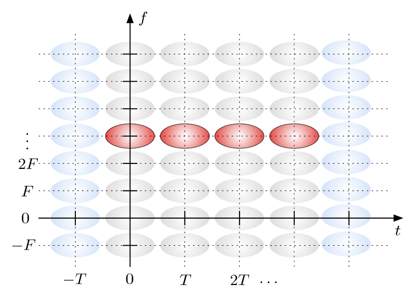
Figure 3: Slots in the time-frequency plane occupied by the symbol $\widetilde{\mathbf{x}}_{3}$ for the case $K^{\prime}=4$.

Steps similar to the one detailed in Appendix G [see (104)] yield the following lower bound on $C_{\infty}$:

$$C_{\infty}=\lim_{N\to\infty}\lim_{K\to\infty}\sup_{\mathcal{S}}\frac{1}{KT}I(\mathbf{y};\mathbf{x})\geq\lim_{N\to\infty}\frac{1}{K^{{}^{\prime}}T}I(\widetilde{\mathbf{y}};\widetilde{\mathbf{x}}).$$ (113)

Since this lower bound holds for any finite $K^{{}^{\prime}}$ we can tighten it if we take the supremum over $K^{{}^{\prime}}$; this leads to

$$C_{\infty}\geq\sup_{K^{{}^{\prime}}}\lim_{N\to\infty}\frac{1}{K^{{}^{\prime}}T}I(\widetilde{\mathbf{y}};\widetilde{\mathbf{x}}).$$ (114)

We next decompose the mutual information in (114) as the difference of KL divergences [81, Eq. (10)]

$$\frac{1}{K^{{}^{\prime}}T}I(\widetilde{\mathbf{y}};\widetilde{\mathbf{x}})=\frac{1}{K^{{}^{\prime}}T}\operatorname{\mathbb{E}}_{\widetilde{\mathbf{x}}}\mathopen{}\left[D\mathopen{}\left(Q_{\widetilde{\mathbf{y}}\,|\,\widetilde{\mathbf{x}}}\|Q_{\widetilde{\mathbf{y}}\,|\,\widetilde{\mathbf{x}}=\mathbf{0}}\right)\right]-\frac{1}{K^{{}^{\prime}}T}D\mathopen{}\left(Q_{\widetilde{\mathbf{y}}}\|Q_{\widetilde{\mathbf{y}}\,|\,\widetilde{\mathbf{x}}=\mathbf{0}}\right)$$ (115)

and evaluate the two terms separately. As $Q_{\widetilde{\mathbf{y}}\,|\,\widetilde{\mathbf{x}}}=\mathcal{CN}\mathopen{}\left(\mathbf{0},\mathbf{I}_{K^{{}^{\prime}}N}+\left(\widetilde{\mathbf{x}}\widetilde{\mathbf{x}}^{H}\right)\operatorname{\odot}\mathbf{R}_{\widetilde{\mathbf{h}}}\right)$, we can use the closed-form expression for the KL divergence of two JPG random vectors $\mathbf{a}\sim\mathcal{CN}\mathopen{}\left(\mathbf{0},\mathbf{R}_{\mathbf{a}}\right)$ and $\mathbf{b}\sim\mathcal{CN}\mathopen{}\left(\mathbf{0},\mathbf{I}\right)$ [14, Eq. (59)]

$$D\mathopen{}\left(\mathcal{CN}\mathopen{}\left(\mathbf{0},\mathbf{R}_{\mathbf{a}}\right)\mathopen{}\left\|\right.\mathcal{CN}\mathopen{}\left(\mathbf{0},\mathbf{I}\right)\right)=\operatorname{tr}\mathopen{}\left(\mathbf{R}_{\mathbf{a}}-\mathbf{I}\right)-\log\det\mathopen{}\left(\mathbf{R}_{\mathbf{a}}\right).$$ (116)

Thus, the expected divergence in (115) can be expressed as

$$\begin{split}\frac{1}{K^{{}^{\prime}}T}\operatorname{\mathbb{E}}_{\widetilde{\mathbf{x}}}\mathopen{}\left[D\mathopen{}\left(Q_{\widetilde{\mathbf{y}}\,|\,\widetilde{\mathbf{x}}}\|Q_{\widetilde{\mathbf{y}}\,|\,\widetilde{\mathbf{x}}=\mathbf{0}}\right)\right]&=\frac{1}{K^{{}^{\prime}}T}\operatorname{\mathbb{E}}_{\widetilde{\mathbf{x}}}\mathopen{}\left[\operatorname{tr}\mathopen{}\left\{\left(\widetilde{\mathbf{x}}\widetilde{\mathbf{x}}^{H}\right)\operatorname{\odot}\mathbf{R}_{\widetilde{\mathbf{h}}}\right\}\right]\\ &\phantom{=}\quad-\frac{1}{K^{{}^{\prime}}T}\operatorname{\mathbb{E}}_{\widetilde{\mathbf{x}}}\mathopen{}\left[\log\det\mathopen{}\left(\mathbf{I}_{K^{{}^{\prime}}N}+\left(\widetilde{\mathbf{x}}\widetilde{\mathbf{x}}^{H}\right)\operatorname{\odot}\mathbf{R}_{\widetilde{\mathbf{h}}}\right)\right]\\ &\stackrel{{\scriptstyle}}{{=}}P-\frac{1}{K^{{}^{\prime}}TN\beta}\sum_{i=0}^{N-1}\log\det\mathopen{}\left(\mathbf{I}_{K^{{}^{\prime}}N}+\left(\widetilde{\mathbf{x}}^{(i)}\left(\widetilde{\mathbf{x}}^{(i)}\right)^{H}\right)\operatorname{\odot}\mathbf{R}_{\widetilde{\mathbf{h}}}\right).\end{split}$$ (117)

The last step follows because each nonzero vector is transmitted with probability $1/(N\beta)$ in the OO-WHK signaling scheme of Definition 16, and because the diagonal entries of $\mathbf{R}_{\widetilde{\mathbf{h}}}$ are normalized to $1$. We next exploit the structure of the signaling scheme, and the fact that the correlation matrix $\mathbf{R}_{\widetilde{\mathbf{h}}}$ is two-level Toeplitz, to simplify the determinant in the second term on the RHS of (117) as

$$\det\mathopen{}\left(\mathbf{I}_{K^{{}^{\prime}}N}+\left(\widetilde{\mathbf{x}}^{(i)}\left(\widetilde{\mathbf{x}}^{(i)}\right)^{H}\right)\operatorname{\odot}\mathbf{R}_{\widetilde{\mathbf{h}}}\right)=\det\mathopen{}\left(\mathbf{I}_{K^{{}^{\prime}}}+\beta PT\mathbf{R}_{\widetilde{\mathbf{h}}}[0]\right)$$ (118)

for all $i$, and where $\widetilde{\mathbf{h}}[0]=\big{[}\begin{matrix}h[0,0]\;h[1,0]\;\cdots\;h[K^{{}^{\prime}}-1,0]\end{matrix}\big{]}\raisebox{0.34444pt}{\vphantom{M}}^{T}$ and $\mathbf{R}_{\widetilde{\mathbf{h}}}[0]=\operatorname{\mathbb{E}}[\widetilde{\mathbf{h}}[0]\widetilde{\mathbf{h}}^{H}[0]]$. We next substitute our intermediate results (115), (117), and (118) into the lower bound (114) to obtain

$$C_{\infty}\geq P-\inf_{K^{{}^{\prime}}}\Biggl{\{}\frac{1}{\beta K^{{}^{\prime}}T}\log\det\mathopen{}\left(\mathbf{I}_{K^{{}^{\prime}}}+\beta PT\mathbf{R}_{\widetilde{\mathbf{h}}}[0]\right)+\lim_{N\to\infty}\frac{1}{K^{{}^{\prime}}T}D\mathopen{}\left(Q_{\widetilde{\mathbf{y}}}\|Q_{\widetilde{\mathbf{y}}\,|\,\widetilde{\mathbf{x}}=\mathbf{0}}\right)\Biggr{\}}.$$ (119)

In Appendix I it is shown that

$$\lim_{N\to\infty}\frac{1}{K^{{}^{\prime}}T}D\mathopen{}\left(Q_{\widetilde{\mathbf{y}}}\|Q_{\widetilde{\mathbf{y}}\,|\,\widetilde{\mathbf{x}}=\mathbf{0}}\right)=0.$$

To conclude, we simplify the second term on the RHS of (119) as

$$\inf_{K^{{}^{\prime}}}\frac{1}{\beta K^{{}^{\prime}}T}\log\det\mathopen{}\left(\mathbf{I}_{K^{{}^{\prime}}}+\beta PT\mathbf{R}_{\widetilde{\mathbf{h}}}[0]\right) \stackrel{{\scriptstyle(a)}}{{=}}\frac{1}{\beta T}\int_{-1/2}^{1/2}\log\mathopen{}\left(1+\beta P\sum_{k=-\infty}^{\infty}q_{\operatorname{\mathbb{H}}}\mathopen{}\left(\frac{\theta+k}{T}\right)\right)d\theta$$

$$\stackrel{{\scriptstyle(b)}}{{=}}\frac{1}{\beta}\int_{\nu}\log\mathopen{}\left(1+\beta Pq_{\operatorname{\mathbb{H}}}(\nu)\right)d\nu.$$

Here, in (a) we used Lemma 11 in Appendix B for the case when $\mathbf{x}$ is a $K^{{}^{\prime}}$-dimensional vector with all-$1$ entries, as well as

$$c(\theta) =\sum_{k=-\infty}^{\infty}R_{\operatorname{\mathbb{H}}}[k,0]e^{-j2\pi k\theta}$$

$$=\iint_{\nu\>\tau}C_{\operatorname{\mathbb{H}}}(\nu,\tau)\sum_{k=-\infty}^{\infty}e^{j2\pi kT\left(\nu-\frac{\theta}{T}\right)}d\tau d\nu$$

$$=\frac{1}{T}\sum_{k=-\infty}^{\infty}q_{\operatorname{\mathbb{H}}}\mathopen{}\left(\frac{\theta-k}{T}\right).$$

Finally, (b) holds because $q_{\operatorname{\mathbb{H}}}(\nu)$ is compactly supported on $[-\nu_{0},\nu_{0}]$, and $T\leq 1/(2\nu_{0})$. A change of variables $\nu=\theta/T$ yields the final result.

Appendix I

Lemma 17

Consider a channel with input-output relation(112)

$$\mathbf{y}=\mathbf{x}\operatorname{\odot}\mathbf{h}+\mathbf{w}$$

where the $K^{{}^{\prime}}N$-dimensional vectors $\mathbf{y}$, $\mathbf{x}$, $\mathbf{h}$, and $\mathbf{w}$ are defined as in (111), i.e., stacking is first along time and then along frequency. Then,

$$\lim_{N\to\infty}\frac{1}{K^{{}^{\prime}}}D\mathopen{}\left(Q_{\mathbf{y}}\|Q_{\mathbf{y}\,|\,\mathbf{x}=\mathbf{0}}\right)=0$$ (120)

for the OO-WHK scheme in Definition 16 of Appendix H.

Proof:

Let $q_{\mathbf{y}}$ and $q_{\mathbf{y}\,|\,\mathbf{x}}$ be the probability density functions (PDFs) associated with the probability distributions $Q_{\mathbf{y}}$ and $Q_{\mathbf{y}\,|\,\mathbf{x}}$, respectively. By definition of the KL divergence,

$$D\mathopen{}\left(Q_{\mathbf{y}}\|Q_{\mathbf{y}\,|\,\mathbf{x}=\mathbf{0}}\right)=\operatorname{\mathbb{E}}_{\mathbf{y}}\mathopen{}\left[\log\mathopen{}\left(\frac{q_{\mathbf{y}}(\mathbf{y})}{q_{\mathbf{y}\,|\,\mathbf{x}=\mathbf{0}}(\mathbf{y})}\right)\right].$$ (121)

For the OO-WHK scheme in Definition 16, the PDF $q_{\mathbf{y}}$ of the output vector can be written as

$$q_{\mathbf{y}}=\left(1-\frac{1}{\beta}\right)q_{\mathbf{y}\,|\,\mathbf{x}=\mathbf{0}}+\frac{1}{N\beta}\sum_{i=0}^{N-1}q_{\mathbf{y}\,|\,\mathbf{x}=\mathbf{x}_{i}}.$$ (122)

The output random vector $\mathbf{y}$ has the same distribution as the noise vector $\mathbf{w}\sim\mathcal{CN}(\mathbf{0},\mathbf{I}_{K^{{}^{\prime}}N})$ when $\mathbf{x}=\mathbf{0}$. Hence, $q_{\mathbf{y}\,|\,\mathbf{x}=\mathbf{0}}=q_{\mathbf{w}}$. To express (121) in a more convenient form, we define the following RV:

$$S_{N}(\mathbf{w})=\sum_{i=0}^{N-1}\underbrace{\left[\left(1-\frac{1}{\beta}\right)+\frac{1}{\beta}\frac{q_{\mathbf{y}\,|\,\mathbf{x}=\mathbf{x}_{i}}(\mathbf{w})}{q_{\mathbf{w}}(\mathbf{w})}\right]}_{s_{i}(\mathbf{w})}.$$

We can express the KL divergence (121) as a function of the RV $S_{N}(\mathbf{w})$ as follows:

$$\operatorname{\mathbb{E}}_{\mathbf{y}}\mathopen{}\left[\log\mathopen{}\left(\frac{q_{\mathbf{y}}(\mathbf{y})}{q_{\mathbf{y}\,|\,\mathbf{x}=\mathbf{0}}(\mathbf{y})}\right)\right] =\int_{\mathbf{y}}\log\mathopen{}\left(\frac{q_{\mathbf{y}}(\mathbf{y})}{q_{\mathbf{y}\,|\,\mathbf{x}=\mathbf{0}}(\mathbf{y})}\right)q_{\mathbf{y}}(\mathbf{y})d\mathbf{y}$$

$$=\int_{\mathbf{y}}\log\mathopen{}\left(\left(1-\frac{1}{\beta}\right)+\frac{1}{N\beta}\sum_{i=0}^{N-1}\frac{q_{\mathbf{y}\,|\,\mathbf{x}=\mathbf{x}_{i}}(\mathbf{y})}{q_{\mathbf{y}\,|\,\mathbf{x}=\mathbf{0}}(\mathbf{y})}\right)$$

$$\phantom{=}\quad\times\left[\left(1-\frac{1}{\beta}\right)q_{\mathbf{y}\,|\,\mathbf{x}=\mathbf{0}}(\mathbf{y})+\frac{1}{N\beta}\sum_{i=0}^{N-1}q_{\mathbf{y}\,|\,\mathbf{x}=\mathbf{x}_{i}}(\mathbf{y})\right]d\mathbf{y}$$

$$=\int_{\mathbf{y}}\frac{S_{N}(\mathbf{y})}{N}\log\mathopen{}\left(\frac{S_{N}(\mathbf{y})}{N}\right)\underbrace{q_{\mathbf{y}\,|\,\mathbf{x}=\mathbf{0}}}_{q_{\mathbf{w}}}(\mathbf{y})d\mathbf{y}$$

$$=\operatorname{\mathbb{E}}_{\mathbf{w}}\mathopen{}\left[\frac{S_{N}(\mathbf{w})}{N}\log\mathopen{}\left(\frac{S_{N}(\mathbf{w})}{N}\right)\right].$$

To prove Lemma 17, it suffices to show that the sequence of RVs $\{V_{N}(\mathbf{w})\}$ where

$$V_{N}(\mathbf{w})=\frac{S_{N}(\mathbf{w})}{N}\log\mathopen{}\left(\frac{S_{N}(\mathbf{w})}{N}\right)$$

converges to $0$ in mean as $N\to\infty$. To prove this result, we first show that $\{V_{N}(\mathbf{w})\}$ converges to $0$ w.p.1. Then we argue that the sequence forms a backward submartingale [82, p. 474 and p. 499] so that it converges to $0$ also in mean by the submartingale convergence theorem [83, Sec. 32.IV].

I-A Convergence w.p.1

The RVs $s_{i}(\mathbf{w})$ are i.i.d. for $i=0,1,\ldots,N-1$. As this result is rather tedious to prove, we postpone its proof to Appendix I-C. It is instead straightforward to prove that these RVs have mean $1$. In fact,

$$\operatorname{\mathbb{E}}_{\mathbf{w}}\mathopen{}\left[s_{i}(\mathbf{w})\right]=\int_{\mathbf{w}}\left[\left(1-\frac{1}{\beta}\right)+\frac{1}{\beta}\frac{q_{\mathbf{y}\,|\,\mathbf{x}=\mathbf{x}_{i}}(\mathbf{w})}{q_{\mathbf{w}}(\mathbf{w})}\right]q_{\mathbf{w}}(\mathbf{w})d\mathbf{w}=1.$$

It then follows from the strong law of large numbers that

$$\lim_{N\to\infty}\frac{S_{N}(\mathbf{w})}{N}=\operatorname{\mathbb{E}}_{\mathbf{w}}\mathopen{}\left[s_{0}(\mathbf{w})\right]=1\quad\text{w.p.1}$$

and, as the function $r\mathopen{}\left(x\right)=x\log x$ is continuous, we have by [78, Th. 4.6] that

$$\lim_{N\to\infty}V_{N}(\mathbf{w})=\lim_{N\to\infty}r\mathopen{}\left(\frac{S_{N}(\mathbf{w})}{N}\right)=r\mathopen{}\left(\lim_{N\to\infty}\frac{S_{N}(\mathbf{w})}{N}\right)=0\quad\text{w.p.1}.$$

I-B Convergence in Mean

As the RVs $\{s_{i}(\mathbf{w})\}$ are i.i.d., the sequence $\{V_{N}(\mathbf{w})\}$ and the decreasing sequence of $\sigma$-fields $\left\{\mathcal{G}_{N}\right\}$, where $\mathcal{G}_{N}$ is the smallest $\sigma$-field with respect to which the random variables $\{S_{N}(\mathbf{w}),S_{N+1}(\mathbf{w}),\cdots\}$ are measurable, form a backward (or reverse) submartingale [82, p. 474 and p. 499]. This result follows because the pair $\left(\left\{S_{N}(\mathbf{w})/N\right\},\{\mathcal{G}_{N}\}\right)$ is a backward martingale [82, p. 499], and because the function $r\mathopen{}\left(x\right)=x\log x$ is convex.

Since $\{V_{N}(\mathbf{w})\}$ is a backward submartingale and $\{V_{N}(\mathbf{w})\}$ converges to $0$ w.p.1 as $N\to\infty$,  $\{V_{N}(\mathbf{w})\}$ converges to $0$ as $N\to\infty$ also in mean. This result follows by the backward submartingale convergence theorem below:

Theorem 18 (see [83, Sec. 32.IV])

Let $\{X_{N}\}$ be a backward submartingale with respect to a decreasing sequence of $\sigma$-fields $\left\{\mathcal{G}_{N}\right\}$. Then $\{X_{N}\}$ converges w.p.1 and in mean to $X<\infty$ if and only if $\operatorname{\mathbb{E}}\mathopen{}\left[\left\lvert X_{1}\right\rvert\right]<\infty$ and $\lim_{N\to\infty}\operatorname{\mathbb{E}}\mathopen{}\left[X_{N}\right]>-\infty$.

To conclude the proof, we need to show that the technical conditions in Theorem 18 hold, i.e., that the sequence $\{V_{N}(\mathbf{w})\}$ satisfies

$$\lim_{N\to\infty}\operatorname{\mathbb{E}}_{\mathbf{w}}\mathopen{}\left[V_{N}(\mathbf{w})\right]>-\infty$$ (123)

and

$$\operatorname{\mathbb{E}}_{\mathbf{w}}\mathopen{}\left[\left\lvert V_{1}(\mathbf{w})\right\rvert\right]=\operatorname{\mathbb{E}}_{\mathbf{w}}\mathopen{}\left[\left\lvert s_{0}(\mathbf{w})\log s_{0}(\mathbf{w})\right\rvert\right]<\infty.$$ (124)

The first inequality follows from Jensen’s inequality and because the $s_{i}(\mathbf{w})$ have mean $1$:

$$\operatorname{\mathbb{E}}_{\mathbf{w}}\mathopen{}\left[V_{N}(\mathbf{w})\right]=\operatorname{\mathbb{E}}_{\mathbf{w}}\mathopen{}\left[r\mathopen{}\left(\frac{S_{N}(\mathbf{w})}{N}\right)\right]\geq r\mathopen{}\left(\operatorname{\mathbb{E}}_{\mathbf{w}}\mathopen{}\left[\frac{S_{N}(\mathbf{w})}{N}\right]\right)=0\quad\forall N.$$

The second inequality is proven in Appendix I-D. ∎

I-C The Random Variables $s_{i}(\mathbf{w})$ are i.i.d.

To show that the RVs

$$s_{i}(\mathbf{w})=\left[\left(1-\frac{1}{\beta}\right)+\frac{1}{\beta}\frac{q_{\mathbf{y}\,|\,\mathbf{x}=\mathbf{x}_{i}}(\mathbf{w})}{q_{\mathbf{w}}(\mathbf{w})}\right]$$

are i.i.d., we first simplify $q_{\mathbf{y}\,|\,\mathbf{x}=\mathbf{x}_{i}}$ as

$$\begin{split}q_{\mathbf{y}\,|\,\mathbf{x}=\mathbf{x}_{i}}(\mathbf{w})&=\frac{\exp\mathopen{}\left[-\mathbf{w}^{H}\left(\mathbf{I}_{K^{{}^{\prime}}N}+\left(\mathbf{x}_{i}\mathbf{x}_{i}^{H}\right)\operatorname{\odot}\mathbf{R}_{\mathbf{h}}\right)^{-1}\mathbf{w}\right]}{\pi^{K^{{}^{\prime}}N}\det\mathopen{}\left(\mathbf{I}_{K^{{}^{\prime}}N}+\left(\mathbf{x}_{i}\mathbf{x}_{i}^{H}\right)\operatorname{\odot}\mathbf{R}_{\mathbf{h}}\right)}\\ &=\dfrac{\exp\biggl{(}\displaystyle-\mathop{\sum_{n=0}^{N-1}}_{n\neq i}\lVert\mathbf{w}[n]\rVert^{2}-\mathbf{w}^{H}[i]\mathbf{A}^{-1}\mathbf{w}[i]\biggr{)}}{\pi^{K^{{}^{\prime}}N}\det(\mathbf{A})}\end{split}$$ (125)

where we set

$$\mathbf{A}=\mathbf{I}_{K^{{}^{\prime}}}+\beta PT\mathbf{R}_{\mathbf{h}}[0]$$ (126)

and where, as usual, $\mathbf{w}=\big{[}\begin{matrix}\mathbf{w}^{T}[0]\;\mathbf{w}^{T}[1]\;\cdots\;\mathbf{w}^{T}[N-1]\end{matrix}\big{]}\raisebox{0.34444pt}{\vphantom{M}}^{T}.$ To obtain (125) we apply the determinant equality (118) to simplify the denominator. For the numerator, we used that, for the OO-WHK in Definition 16, the matrix $\mathbf{I}_{K^{{}^{\prime}}N}+\left(\mathbf{x}_{i}\mathbf{x}_{i}^{H}\right)\operatorname{\odot}\mathbf{R}_{\mathbf{h}}$ is block diagonal, with $N-1$ blocks equal to $\mathbf{I}_{K^{{}^{\prime}}}$ and one block equal to $\mathbf{A}=\mathbf{I}_{K^{{}^{\prime}}}+\beta PT\mathbf{R}_{\mathbf{h}}[0]$. Hence, its inverse is also block diagonal, with $N-1$ blocks equal to $\mathbf{I}_{K^{{}^{\prime}}}$ and one block equal to $\mathbf{A}^{-1}$. Next, we use (125) to express the ratio $q_{\mathbf{y}\,|\,\mathbf{x}=\mathbf{x}_{i}}/q_{\mathbf{w}}$ as

$$\frac{q_{\mathbf{y}\,|\,\mathbf{x}=\mathbf{x}_{i}}(\mathbf{w})}{q_{\mathbf{w}}(\mathbf{w})}=\frac{1}{\det\mathopen{}\left(\mathbf{A}\right)}\exp\mathopen{}\left[\lVert\mathbf{w}[i]\rVert^{2}-\mathbf{w}^{H}[i]\mathbf{A}^{-1}\mathbf{w}[i]\right].$$ (127)

This last result implies that each $s_{i}(\mathbf{w})$ depends only on the random noise vector $\mathbf{w}[i]$. As the noise is white, the random vectors $\mathbf{w}[i]$ are i.i.d. for all $i$. Hence, the RVs $s_{i}(\mathbf{w})$ are i.i.d. as well.

I-D Proof of Inequality (124)

As $x\log x\geq-e^{-1}$ for all $x>0$, we have that $\left\lvert x\log x\right\rvert\leq x\log x+2e^{-1}$; hence,

$$\operatorname{\mathbb{E}}_{\mathbf{w}}\mathopen{}\left[\left\lvert s_{0}(\mathbf{w})\log s_{0}(\mathbf{w})\right\rvert\right]\leq\operatorname{\mathbb{E}}_{\mathbf{w}}\mathopen{}\left[s_{0}(\mathbf{w})\log s_{0}(\mathbf{w})\right]+2e^{-1}.$$

We next use the convexity of $x\log x$ and that $\beta\geq 1$ to upper-bound $s_{0}(\mathbf{w})\log s_{0}(\mathbf{w})$ as

$$\begin{split}s_{0}(\mathbf{w})\log s_{0}(\mathbf{w})&=\left[\left(1-\frac{1}{\beta}\right)+\frac{1}{\beta}\frac{q_{\mathbf{y}\,|\,\mathbf{x}=\mathbf{x}_{0}}(\mathbf{w})}{q_{\mathbf{w}}(\mathbf{w})}\right]\log\mathopen{}\left[\left(1-\frac{1}{\beta}\right)+\frac{1}{\beta}\frac{q_{\mathbf{y}\,|\,\mathbf{x}=\mathbf{x}_{0}}(\mathbf{w})}{q_{\mathbf{w}}(\mathbf{w})}\right]\\ &\stackrel{{\scriptstyle(a)}}{{\leq}}\frac{1}{\beta}\left[\frac{q_{\mathbf{y}\,|\,\mathbf{x}=\mathbf{x}_{0}}(\mathbf{w})}{q_{\mathbf{w}}(\mathbf{w})}\right]\log\mathopen{}\left[\frac{q_{\mathbf{y}\,|\,\mathbf{x}=\mathbf{x}_{0}}(\mathbf{w})}{q_{\mathbf{w}}(\mathbf{w})}\right]\\ &\stackrel{{\scriptstyle(b)}}{{\leq}}\left[\frac{q_{\mathbf{y}\,|\,\mathbf{x}=\mathbf{x}_{0}}(\mathbf{w})}{q_{\mathbf{w}}(\mathbf{w})}\right]\log\mathopen{}\left[\frac{q_{\mathbf{y}\,|\,\mathbf{x}=\mathbf{x}_{0}}(\mathbf{w})}{q_{\mathbf{w}}(\mathbf{w})}\right]\end{split}$$ (128)

where (a) follows from the definition of convexity, and in (b) we used that $\beta\geq 1$. If we take the expectation on both sides of (128), we get

$$\operatorname{\mathbb{E}}\mathopen{}\left[s_{0}(\mathbf{w})\log s_{0}(\mathbf{w})\right] \leq\int_{\mathbf{w}}\left[\frac{q_{\mathbf{y}\,|\,\mathbf{x}=\mathbf{x}_{0}}(\mathbf{w})}{q_{\mathbf{w}}(\mathbf{w})}\right]\log\mathopen{}\left[\frac{q_{\mathbf{y}\,|\,\mathbf{x}=\mathbf{x}_{0}}(\mathbf{w})}{q_{\mathbf{w}}(\mathbf{w})}\right]q_{\mathbf{w}}(\mathbf{w})d\mathbf{w}$$

$$\stackrel{{\scriptstyle(a)}}{{\leq}}\int_{\mathbf{w}}q_{\mathbf{y}\,|\,\mathbf{x}=\mathbf{x}_{0}}(\mathbf{w})\left\lvert\log\mathopen{}\left[\frac{q_{\mathbf{y}\,|\,\mathbf{x}=\mathbf{x}_{0}}(\mathbf{w})}{q_{\mathbf{w}}(\mathbf{w})}\right]\right\rvert d\mathbf{w}$$

$$\stackrel{{\scriptstyle(b)}}{{=}}\int_{\mathbf{w}}\frac{\exp\mathopen{}\left(-\sum_{n=1}^{N-1}\lVert\mathbf{w}[n]\rVert^{2}-\mathbf{w}^{H}[0]\mathbf{A}^{-1}\mathbf{w}[0]\right)}{\pi^{K^{{}^{\prime}}N}\det(\mathbf{A})}$$

$$\hphantom{=\int_{\mathbf{w}}}\times\left\lvert\log\mathopen{}\left(\frac{\exp\mathopen{}\left(\lVert\mathbf{w}[0]\rVert^{2}-\mathbf{w}[0]^{H}\mathbf{A}^{-1}\mathbf{w}[0]\right)}{\det(\mathbf{A})}\right)\right\rvert d\mathbf{w}$$

$$\stackrel{{\scriptstyle(c)}}{{\leq}}\int_{\mathbf{w}[0]}\frac{\exp\mathopen{}\left(-\mathbf{w}^{H}[0]\mathbf{A}^{-1}\mathbf{w}[0]\right)}{\pi^{K^{{}^{\prime}}}\det(\mathbf{A})}$$

$$\hphantom{=\int_{\mathbf{w}}}\times\left[\lVert\mathbf{w}[0]\rVert^{2}+\mathbf{w}[0]^{H}\mathbf{A}^{-1}\mathbf{w}[0]+\log\mathopen{}\left(\det\mathopen{}\left(\mathbf{A}\right)\right)\right]d\mathbf{w}[0]$$

$$<\infty.$$

where (a) follows because $q_{\mathbf{y}\,|\,\mathbf{x}=\mathbf{x}_{0}}(\mathbf{w})>0$ for all $\mathbf{w}$; in (b) we used (125) and (127), while to obtain (c) we first integrated over $\{\mathbf{w}[n]\}_{n=1}^{N-1}$ and then we used the triangle inequality and that $\mathbf{A}$ is positive definite with eigenvalues larger or equal to $1$ [see (126)]. The last inequality holds because $\mathbf{A}$ satisfies the trace constraint $\operatorname{tr}(\mathbf{A})=K^{{}^{\prime}}(1+\beta PT)$, which implies that its eigenvalues are bounded.

Appendix J Proof of Theorem 8

We use the decomposition of mutual information as a difference of KL divergences (115), and upper-bound $\sup_{\mathcal{S}}I(\mathbf{y};\mathbf{x})$ in (56) because the KL divergence is nonnegative:

$$\sup_{\mathcal{S}}I(\mathbf{y};\mathbf{x}) =\sup_{\mathcal{S}}\left\{\operatorname{\mathbb{E}}_{\mathbf{x}}\mathopen{}\left[D\mathopen{}\left(Q_{\mathbf{y}\,|\,\mathbf{x}}\|Q_{\mathbf{y}\,|\,\mathbf{x}=\mathbf{0}}\right)\right]-D\mathopen{}\left(Q_{\mathbf{y}}\|Q_{\mathbf{y}\,|\,\mathbf{x}=\mathbf{0}}\right)\right\}$$ (129)

$$\leq\sup_{\mathcal{S}}\operatorname{\mathbb{E}}_{\mathbf{x}}\mathopen{}\left[D\mathopen{}\left(Q_{\mathbf{y}\,|\,\mathbf{x}}\|Q_{\mathbf{y}\,|\,\mathbf{x}=\mathbf{0}}\right)\right].$$ (130)

As in the proof of Theorem 1, we rewrite the supremum over the distributions in the set $\mathcal{S}$ as a double supremum over $\alpha\in[0,1]$ and over the restricted set of input distributions $\mathcal{S}\rvert_{\alpha}$ that satisfy the average power constraint $\operatorname{\mathbb{E}}\mathopen{}\left[\lVert\mathbf{x}\rVert^{2}\right]=\alpha KP\,T$ and the peak constraint (23). Then, we use the closed-form expression for the KL divergence of two multivariate Gaussian vectors (116) and we follow the same arguments as in the proof of Theorem 1:

$$\frac{1}{KT}\sup_{\mathcal{S}} \operatorname{\mathbb{E}}_{\mathbf{x}}\mathopen{}\left[D\mathopen{}\left(Q_{\mathbf{y}\,|\,\mathbf{x}}\|Q_{\mathbf{y}\,|\,\mathbf{x}=\mathbf{0}}\right)\right]$$

$$=\sup_{0\leq\alpha\leq 1}\sup_{\mathcal{S}\rvert_{\alpha}}\left\{\alpha P-\frac{1}{KT}\operatorname{\mathbb{E}}\mathopen{}\left[\log\det\mathopen{}\left(\mathbf{I}_{KN}+\left(\mathbf{x}\mathbf{x}^{H}\right)\operatorname{\odot}\mathbf{R}_{\mathbf{h}}\right)\right]\right\}$$

$$=\sup_{0\leq\alpha\leq 1}\left\{\alpha P-\inf_{\mathcal{S}\rvert_{\alpha}}\frac{1}{KT}\operatorname{\mathbb{E}}\mathopen{}\left[\log\det\mathopen{}\left(\mathbf{I}_{KN}+\left(\mathbf{x}\mathbf{x}^{H}\right)\operatorname{\odot}\mathbf{R}_{\mathbf{h}}\right)\right]\right\}$$

$$\leq\sup_{0\leq\alpha\leq 1}\left\{\alpha P-\alpha P\inf_{\mathbf{x}}\frac{\log\det\mathopen{}\left(\mathbf{I}_{KN}+\left(\mathbf{x}\mathbf{x}^{H}\right)\operatorname{\odot}\mathbf{R}_{\mathbf{h}}\right)}{\lVert\mathbf{x}\rVert^{2}}\right\}$$

$$=P-P\inf_{\mathbf{x}}\frac{\log\det\mathopen{}\left(\mathbf{I}_{KN}+\left(\mathbf{x}\mathbf{x}^{H}\right)\operatorname{\odot}\mathbf{R}_{\mathbf{h}}\right)}{\lVert\mathbf{x}\rVert^{2}}.$$ (131)

The infimum in (131) has the same structure as the infimum (33) in the proof of Theorem 1. Hence, as $\mathbf{R}_{\mathbf{h}}$ is positive semidefinite, we can conclude that the infimum (131) is achieved on the boundary of the admissible set. Differently from the proof of Theorem 1, however, the input signal is subject to a peak constraint in time so that the admissible set is defined by the two conditions

$$\begin{split}\left\lvert x[k,n]\right\rvert^{2}&\in\{0,\beta PT\}\\ \sum_{n=0}^{N-1}\left\lvert x[k,n]\right\rvert^{2}&\leq\beta PT,\quad\text{w.p.1}.\end{split}$$ (132)

Hence, a necessary condition for a vector $\mathbf{x}$ to minimize $\log\det\mathopen{}\left(\mathbf{I}_{KN}+\left(\mathbf{x}\mathbf{x}^{H}\right)\operatorname{\odot}\mathbf{R}_{\mathbf{h}}\right)/\lVert\mathbf{x}\rVert^{2}$ is the following: for any fixed $k$, $x[k,n]$ may be different from $0$ only for at most one discrete frequency $n$. An example of such a vector is shown in Fig. 4.

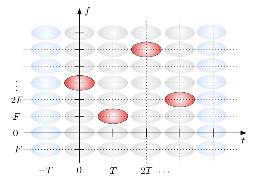
Figure 4: The entries in the time-frequency plane of a vector $\mathbf{x}$ that satisfies the necessary condition to minimize $\log\det\mathopen{}\left(\mathbf{I}_{KN}+\left(\mathbf{x}\mathbf{x}^{H}\right)\operatorname{\odot}\mathbf{R}_{\mathbf{h}}\right)/\lVert\mathbf{x}\rVert^{2}$ in (132) for the case $K=4$.

Even if the structure of the vector minimizing the second term on the RHS of (131) is known, the infimum (131) does not seem to admit a closed-form expression. We can obtain, however, the following closed-form lower bound on the infimum if we replace the constraint $\sum_{n=0}^{N-1}\left\lvert x[k,n]\right\rvert^{2}\leq\beta PT$ w.p.1 in (132) with the less stringent constraint $\left\lvert x[k,n]\right\rvert^{2}\leq\beta PT$ w.p.1 for all $k$ and $n$. The infimum of $\log\det\mathopen{}\left(\mathbf{I}_{KN}+\left(\mathbf{x}\mathbf{x}^{H}\right)\operatorname{\odot}\mathbf{R}_{\mathbf{h}}\right)/\lVert\mathbf{x}\rVert^{2}$ over the vectors $\mathbf{x}$ that belong to the new admissible set can be bounded as in (34), after replacing $\beta PT/N$ by $\beta PT$ and proceeding as in (17):

$$\begin{split}\inf_{\mathbf{x}}\frac{1}{\lVert\mathbf{x}\rVert^{2}}\log\det\mathopen{}\left(\mathbf{I}_{KN}+\left(\mathbf{x}\mathbf{x}^{H}\right)\operatorname{\odot}\mathbf{R}_{\mathbf{h}}\right)&\geq\frac{1}{\beta PT}\int_{-1/2}^{1/2}\int_{-1/2}^{1/2}\log\mathopen{}\left(1+\beta PTc(\theta,\varphi)\right)d\theta d\varphi\\ &=\frac{F}{\beta P}\iint_{\nu\>\tau}\log\mathopen{}\left(1+\frac{\beta P}{F}C_{\operatorname{\mathbb{H}}}(\nu,\tau)\right)d\tau d\nu.\end{split}$$ (133)

To conclude the proof, we substitute (133) in (131) and obtain the desired upper bound (58).

References

• [1] E. Biglieri, J. Proakis, and S. Shamai (Shitz), “Fading channels: Information-theoretic and communications aspects,” IEEE Trans. Inf. Theory, vol. 44, no. 6, pp. 2619–2692, Oct. 1998.
• [2] R. Vaughan and J. Bach Andersen, Channels, Propagation and Antennas for Mobile Communications.   London, U.K.: The Institution of Electrical Engineers, 2003.
• [3] D. N. C. Tse and P. Viswanath, Fundamentals of Wireless Communication.   Cambridge, U.K.: Cambridge Univ. Press, 2005.
• [4] P. R. Gray, P. J. Hurst, S. H. Lewis, and R. G. Meyer, Analysis and Design of Analog Integrated Circuits, 4th ed.   New York, NY, U.S.A.: Wiley, 2001.
• [5] A. Lapidoth, “On the asymptotic capacity of stationary Gaussian fading channels,” IEEE Trans. Inf. Theory, vol. 51, no. 2, pp. 437–446, Feb. 2005.
• [6] M. Médard, “The effect upon channel capacity in wireless communications of perfect and imperfect knowledge of the channel,” IEEE Trans. Inf. Theory, vol. 46, no. 3, pp. 933–946, May 2000.
• [7] I. E. Telatar and D. N. C. Tse, “Capacity and mutual information of wideband multipath fading channels,” IEEE Trans. Inf. Theory, vol. 46, no. 4, pp. 1384–1400, Jul. 2000.
• [8] M. Médard and R. G. Gallager, “Bandwidth scaling for fading multipath channels,” IEEE Trans. Inf. Theory, vol. 48, no. 4, pp. 840–852, Apr. 2002.
• [9] V. G. Subramanian and B. Hajek, “Broad-band fading channels: Signal burstiness and capacity,” IEEE Trans. Inf. Theory, vol. 48, no. 4, pp. 809–827, Apr. 2002.
• [10] I. M. Jacobs, “The asymptotic behavior of incoherent M-ary communication systems,” Proc. IEEE, vol. 51, no. 1, pp. 251–252, Jan. 1963.
• [11] J. R. Pierce, “Ultimate performance of ${M}$-ary transmission on fading channels,” IEEE Trans. Inf. Theory, vol. 12, no. 1, pp. 2–5, Jan. 1966.
• [12] R. S. Kennedy, Fading Dispersive Communication Channels.   New York, NY, U.S.A.: Wiley, 1969.
• [13] R. G. Gallager, Information Theory and Reliable Communication.   New York, NY, U.S.A.: Wiley, 1968.
• [14] S. Verdú, “Spectral efficiency in the wideband regime,” IEEE Trans. Inf. Theory, vol. 48, no. 6, pp. 1319–1343, Jun. 2002.
• [15] G. Durisi, H. Bölcskei, and S. Shamai (Shitz), “Capacity of underspread WSSUS fading channels in the wideband regime,” in Proc. IEEE Int. Symp. Inf. Theory (ISIT), Seattle, WA, U.S.A., Jul. 2006, pp. 1500–1504.
• [16] P. A. Bello, “Characterization of randomly time-variant linear channels,” IEEE Trans. Commun., vol. 11, no. 4, pp. 360–393, Dec. 1963.
• [17] A. M. Sayeed and B. Aazhang, “Joint multipath-Doppler diversity in mobile wireless communications,” IEEE Trans. Commun., vol. 47, no. 1, pp. 123–132, Jan. 1999.
• [18] X. Ma and G. B. Giannakis, “Maximum-diversity transmission over doubly selective wireless channels,” IEEE Trans. Inf. Theory, vol. 49, no. 7, pp. 1832–1840, Jul. 2003.
• [19] T. Zemen and C. F. Mecklenbräuker, “Time-variant channel estimation using discrete prolate spheroidal sequences,” IEEE Trans. Signal Process., vol. 53, no. 9, pp. 3597–3607, Sep. 2005.
• [20] W. Kozek, “Matched Weyl-Heisenberg expansions of nonstationary environments,” Ph.D. dissertation, Vienna University of Technology, Department of Electrical Engineering, Vienna, Austria, Mar. 1997.
• [21] A. Lapidoth and P. Narayan, “Reliable communication under channel uncertainty,” IEEE Trans. Inf. Theory, vol. 44, no. 6, pp. 2148–2177, Oct. 1998.
• [22] I. C. Abou-Faycal, M. D. Trott, and S. Shamai (Shitz), “The capacity of discrete-time memoryless Rayleigh-fading channels,” IEEE Trans. Inf. Theory, vol. 47, no. 4, pp. 1290–1301, May 2001.
• [23] A. J. Viterbi, “Performance of an M-ary orthogonal communication system using stationary stochastic signals,” IEEE Trans. Inf. Theory, vol. 13, no. 3, pp. 414–422, Jul. 1967.
• [24] V. Sethuraman and B. Hajek, “Low SNR capacity of fading channels with peak and average power constraints,” in Proc. IEEE Int. Symp. Inf. Theory (ISIT), Seattle, WA, U.S.A., Jul. 2006, pp. 689–693.
• [25] W. Zhang and J. N. Laneman, “How good is PSK for peak-limited fading channels in the low-SNR regime?” IEEE Trans. Inf. Theory, vol. 53, no. 1, pp. 236–251, Jan. 2007.
• [26] V. Sethuraman and B. Hajek, “Capacity per unit energy of fading channels with peak constraint,” IEEE Trans. Inf. Theory, vol. 51, no. 9, pp. 3102–3120, Sep. 2005.
• [27] V. Sethuraman, B. Hajek, and K. Narayanan, “Capacity bounds for noncoherent fading channels with a peak constraint,” in Proc. IEEE Int. Symp. Inf. Theory (ISIT), Adelaide, Australia, Sep. 2005, pp. 515–519.
• [28] V. Sethuraman, L. Wang, B. Hajek, and A. Lapidoth, “Low SNR capacity of noncoherent fading channels,” IEEE Trans. Inf. Theory, 2008, submitted. [Online]. Available: http://arxiv.org/abs/0712.2872
• [29] D. Schafhuber, H. Bölcskei, and G. Matz, “System capacity of wideband OFDM communications over fading channels without channel knowledge,” in Proc. IEEE Int. Symp. Inf. Theory (ISIT), Chicago, IL, U.S.A., Jun. 2004, p. 391, corrected version online. [Online]. Available: http://www.nari.ee.ethz.ch/commth/pubs/p/ofdm04
• [30] M. Borgmann and H. Bölcskei, “On the capacity of noncoherent wideband MIMO-OFDM systems,” in Proc. IEEE Int. Symp. Inf. Theory (ISIT), Adelaide, Australia, Sep. 2005, pp. 651–655.
• [31] U. Grenander and G. Szegö, Toeplitz Forms and Their Applications.   New York, NY, U.S.A.: Chelsea Publishing, 1984.
• [32] R. M. Gray, “Toeplitz and circulant matrices: A review,” in Foundations and Trends in Communications and Information Theory.   Delft, The Netherlands: now Publishers, 2005, vol. 2, no. 3.
• [33] P. A. Voois, “A theorem on the asymptotic eigenvalue distribution of Toeplitz-block-Toeplitz matrices,” IEEE Trans. Signal Process., vol. 44, no. 7, pp. 1837–1841, Jul. 1996.
• [34] M. Miranda and P. Tilli, “Asymptotic spectra of Hermitian block Toeplitz matrices and preconditioning results,” SIAM J. Matrix Anal. Appl., vol. 21, no. 3, pp. 867–881, Feb. 2000.
• [35] D. Guo, S. Shamai (Shitz), and S. Verdú, “Mutual information and minimum mean-square error in Gaussian channels,” IEEE Trans. Inf. Theory, vol. 51, no. 4, pp. 1261–1282, Apr. 2005.
• [36] S. Butman and M. J. Klass, “Capacity of noncoherent channels,” Jet Propulsion Laboratory, Pasadena, CA, U.S.A., Tech. Rep. 32-1526, Sep. 1973.
• [37] A. W. Naylor and G. R. Sell, Linear Operator Theory in Engineering and Science.   New York, NY, U.S.A.: Springer, 1982.
• [38] N. Dunford and J. T. Schwarz, Linear Operators.   New York, NY, U.S.A.: Wiley, 1963, vol. 2.
• [39] P. D. Lax, Functional Analysis.   New York, NY, U.S.A.: Wiley, 2002.
• [40] U. G. Schuster and H. Bölcskei, “Ultrawideband channel modeling on the basis of information-theoretic criteria,” IEEE Trans. Wireless Commun., vol. 6, no. 7, pp. 2464–2475, Jul. 2007.
• [41] J. G. Proakis, Digital Communications, 4th ed.   New York, NY, U.S.A.: McGraw-Hill, 2001.
• [42] G. Matz and F. Hlawatsch, “Time-frequency characterization of randomly time-varying channels,” in Time-Frequency Signal Analysis and Processing: A Comprehensive Reference, B. Boashash, Ed.   Oxford, U.K.: Elsevier, 2003, ch. 9.5, pp. 410–419.
• [43] D. C. Cox, “A measured delay-Doppler scattering function for multipath propagation at 910 MHz in an urban mobile radio environment,” Proc. IEEE, vol. 61, no. 4, pp. 479–480, Apr. 1973.
• [44] ——, “910 MHz urban mobile radio propagation: Multipath characteristics in New York City,” IEEE Trans. Commun., vol. 21, no. 11, pp. 1188–1194, Nov. 1973.
• [45] W. C. Jakes, Ed., Microwave Mobile Communications.   New York, NY, U.S.A.: Wiley, 1974.
• [46] N. T. Gaarder, “Scattering function estimation,” IEEE Trans. Inf. Theory, vol. 14, no. 5, pp. 684–693, Sep. 1968.
• [47] H. Artés, G. Matz, and F. Hlawatsch, “Unbiased scattering function estimators for underspread channels and extension to data-driven operation,” IEEE Trans. Signal Process., vol. 52, no. 5, pp. 1387–1402, May 2004.
• [48] R. G. Gallager, Principles of Digital Communications.   Cambridge, U.K.: Cambridge Univ. Press, 2008.
• [49] H. Hashemi, “The indoor radio propagation channel,” Proc. IEEE, vol. 81, no. 7, pp. 943–968, Jul. 1993.
• [50] J. D. Parsons, The Mobile Radio Propagation Channel, 2nd ed.   Chichester, U.K.: Wiley, 2000.
• [51] T. S. Rappaport, Wireless Communications: Principles and Practice, 2nd ed.   Upper Saddle River, NJ, U.S.A.: Prentice Hall, 2002.
• [52] T. Kailath, “Time-variant communication channels,” IEEE Trans. Inf. Theory, vol. 9, no. 4, pp. 233–237, Oct. 1963.
• [53] G. E. Pfander and D. F. Walnut, “Measurement of time-variant linear channels,” IEEE Trans. Inf. Theory, vol. 52, no. 11, pp. 4808–4820, Nov. 2006.
• [54] O. Christensen, An Introduction to Frames and Riesz Bases.   Boston, MA, U.S.A.: Birkhäuser, 2003.
• [55] K. Gröchenig, Foundations of Time-Frequency Analysis.   Boston, MA, U.S.A.: Birkhäuser, 2001.
• [56] W. Kozek and A. F. Molisch, “Nonorthogonal pulseshapes for multicarrier communications in doubly dispersive channels,” IEEE J. Sel. Areas Commun., vol. 16, no. 8, pp. 1579–1589, Oct. 1998.
• [57] K. Liu, T. Kadous, and A. Sayeed, “Orthogonal time-frequency signaling over doubly dispersive channels,” IEEE Trans. Inf. Theory, vol. 50, no. 11, pp. 2583–2603, Nov. 2004.
• [58] G. Matz, D. Schafhuber, K. Gröchenig, M. Hartmann, and F. Hlawatsch, “Analysis, optimization, and implementation of low-interference wireless multicarrier systems,” IEEE Trans. Wireless Commun., vol. 6, no. 5, pp. 1921–1931, May 2007.
• [59] G. Matz, “A time-frequency calculus for time-varying systems and nonstationary processes with applications,” Ph.D. dissertation, Vienna University of Technology, Vienna, Austria, Nov. 2000.
• [60] G. Maruyama, “The harmonic analysis of stationary stochastic processes,” Memoirs of the Faculty of Science, Kyūshū University, Ser. A, vol. 4, no. 1, pp. 45–106, 1949.
• [61] R. M. Gray, Entropy and Information Theory, revised ed.   New York, NY, U.S.A.: Springer, 2007. [Online]. Available: http://ee.stanford.edu/~gray/it.pdf
• [62] G. Taricco and M. Elia, “Capacity of fading channel with no side information,” Electron. Lett., vol. 33, no. 16, pp. 1368–1370, Jul. 1997.
• [63] A. Lapidoth and S. M. Moser, “Capacity bounds via duality with applications to multiple-antenna systems on flat-fading channels,” IEEE Trans. Inf. Theory, vol. 49, no. 10, pp. 2426–2467, Oct. 2003.
• [64] R. A. Horn and C. R. Johnson, Matrix Analysis.   Cambridge, U.K.: Cambridge Univ. Press, 1985.
• [65] W. He and C. N. Georghiades, “Computing the capacity of a MIMO fading channel under PSK signaling,” IEEE Trans. Inf. Theory, vol. 51, no. 5, pp. 1794–1803, May 2005.
• [66] B. Razavi, RF Microelectronics.   Upper Saddle River, NJ, U.S.A.: Prentice Hall, 1998.
• [67] M. C. Gursoy, H. V. Poor, and S. Verdú, “On-off frequency-shift keying for wideband fading channels,” EURASIP J. Wireless Commun. Netw., vol. 2006, 2006, article ID 98564.
• [68] U. G. Schuster, G. Durisi, H. Bölcskei, and H. V. Poor, “Capacity bounds for peak-constrained multiantenna wideband channels,” IEEE Trans. Commun., Jan. 2008, submitted. [Online]. Available: http://arxiv.org/abs/0801.1002
• [69] Y. Liang and V. V. Veeravalli, “Capacity of noncoherent time-selective Rayleigh-fading channels,” IEEE Trans. Inf. Theory, vol. 50, no. 12, pp. 3096–3110, Dec. 2004.
• [70] J. Chen and V. V. Veeravalli, “Capacity results for block-stationary Gaussian fading channels with a peak power constraint,” IEEE Trans. Inf. Theory, vol. 53, no. 12, pp. 4498–4520, Dec. 2007.
• [71] T. Koch and A. Lapidoth, “Multipath channels of bounded capacity,” in IEEE Inf. Theory Workshop (ITW), Porto, Portugal, May 2008, to be presented. [Online]. Available: http://arxiv.org/abs/0711.3152
• [72] G. Matz and F. Hlawatsch, “Time-frequency transfer function calculus (symbolic calculus) of linear time-varying systems (linear operators) based on a generalized underspread theory,” J. Math. Phys., vol. 39, no. 8, pp. 4041–4070, Aug. 1998.
• [73] P. M. Woodward, Probability and Information Theory, with Applications to Radar.   London, U.K.: Pergamon Press, 1953.
• [74] C. H. Wilcox, “The synthesis problem for radar ambiguity functions,” in Radar and Sonar, R. E. Blahut, W. Miller, Jr., and C. H. Wilcox, Eds.   New York, NY, U.S.A.: Springer, 1991, vol. 1, pp. 229–260.
• [75] H. V. Poor, An Introduction to Signal Detection and Estimation, 2nd ed.   New York, NY, U.S.A.: Springer, 1994.
• [76] C. W. Helstrom, “Image restoration by the method of least squares,” J. Opt. Soc. Am., vol. 57, pp. 297–303, Mar. 1967.
• [77] J. Pearl, “On coding and filtering stationary signals by discrete Fourier transforms,” IEEE Trans. Inf. Theory, vol. 19, no. 2, pp. 229–232, Mar. 1973.
• [78] W. Rudin, Principles of Mathematical Analysis, 3rd ed.   New York, NY, U.S.A.: McGraw-Hill, 1976.
• [79] V. V. Prelov and S. Verdú, “Second-order asymptotics of mutual information,” IEEE Trans. Inf. Theory, vol. 50, no. 8, pp. 1567–1580, Aug. 2004.
• [80] H. Lütkepohl, Handbook of Matrices.   Chichester, U.K.: Wiley, 1996.
• [81] S. Verdú, “On channel capacity per unit cost,” IEEE Trans. Inf. Theory, vol. 36, no. 5, pp. 1019–1030, Sep. 1990.
• [82] G. R. Grimmett and D. R. Stirzaker, Probability and Random Processes, 3rd ed.   Oxford, U.K.: Oxford Univ. Press, 2001.
• [83] M. Loève, Probability Theory, 4th ed.   New York, NY, U.S.A.: Springer, 1977, vol. 2.