Robust control of a bimorph mirror
for adaptive optics system

Abstract

We apply robust control technics to an adaptive optics system including a dynamic model of the deformable mirror. The dynamic model of the mirror is a modification of the usual plate equation. We propose also a state-space approach to model the turbulent phase. A continuous time control of our model is suggested taking into account the frequential behavior of the turbulent phase. An $H_{\infty}$ controller is designed in an infinite dimensional setting. Due to the multivariable nature of the control problem involved in adaptive optics systems, a significant improvement is obtained with respect to traditional single input single output methods.

Keywords: Adaptive Optics, Robust control, Partial differential equations.

OCIS: 010.1330, 120.4640.

1 Introduction

For several decades it has been now possible to use adaptive optic (AO) systems to actively correct the distortions affecting an incident wavefront propagating through a turbulent medium. A particularly interesting application of this technique is in the field of astronomical ground-based imaging. The idea behind AO systems is to generate a corrected wavefront as close as possible to the genuine incident plane wavefront thanks to a deformable mirror (DM). An AO system is also composed of a wavefront sensor measuring the resulting distortion of the collected wavefront after correction by the DM. Based on these measured signals, the voltage applied to the piezoelectric actuators is computed in order to reshape the mirror. The tilts (first order modes) of the wavefront are corrected by a first mirror. Then, the DM is part of the control-loop for the correction of higher-order modes of the wave front. Different types of sensors (curvature sensor, pyramid wavefront sensor) may be used to estimate the distortions affecting the incoming wave-front but the most common encountered in existing applications is the Shack-Hartmann (SH) sensor. There also exists different type of deformable mirrors and we choose to study the case of the most common one. For additional details on basic principles of adaptive optics, see [1], e.g..

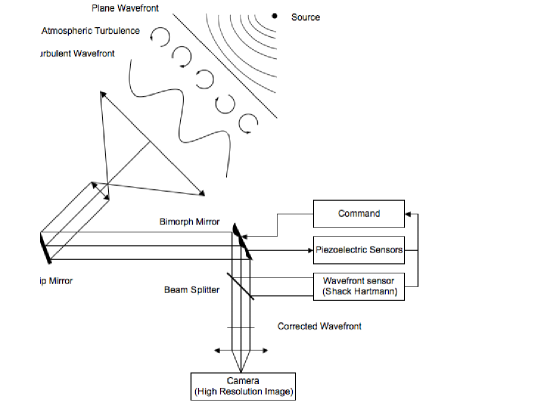
Figure 1: An adaptive optics system - The control loop consists in a SH sensor analyzing the incoming wavefront and a layer of piezoelectric sensors giving the precise position of the bimorph mirror, both of them allowing the calculation of the appropriate command of the DM in order to recover the genuine wavefront.

This paper is devoted to the design of control laws for an adaptive optics system formed by a bimorph mirror and a Shack-Hartmann sensor (see Figure 1). Most often, the existing adaptive optics systems use static models and very basic control algorithms based on frequent measurements of the influence of each actuator of the mirror to each output of the SH. This allows the computation of an interaction matrix gathering the corresponding influence functions. Here, our goal is to consider the design of an adaptive optics system control loop from a modern automatic control point of view as in [2] and [3]. This means first that dynamics of the different elements involved in the control-loop have to be taken into account. In particular, a specific dynamic model for the DM is proposed for control purpose (as already presented in [4] and see also [5]). Secondly, a state-space model of the turbulent phase, built from its frequency domain characteristics, is defined [6].

The main contribution concerns the infinite dimension setting introduced in this paper. More precisely, while in the literature, only static finite dimensional models are considered, a model based on a particular partial differential equation (pde) is used for the DM. We believe that our point of view matches well with the reduction of the size of the actuators and the significant augmentation of their numbers in many devices, as in AO for Very Large Telescopes.

In reference [7], a thin elastic plate model of a deformable bimorph mirror is derived. This model is based on a periodic distribution of embedded piezoelectric patches that may be used as sensors or actuators. The idea is then to elaborate a robust control strategy based on modern control tools for distributed parameter systems [8]. Moreover, in contrast to [9] and [2], we do not need to compute any interaction matrix modelling the relation between the input on the piezoelectric patches attached to the mirror and the output given by the Shack-Hartmann sensor. The interaction matrix can be seen as a static model of the mirror whereas a more general dynamical model of the mirror is used here.

For the sake of clarity of this study, we emphasize here the main informations about the frame we choose for our modeling of robust control of an AO system. We consider a continuous time state-space model of an AO loop (as in [5] and instead of a discrete one in [2] and [9]) and without delay. In practice an AO system uses discrete wavefront sensing data with inherent temporal delays and of course it is possible to derive a discrete time extension of our model but it is not our point here, even if we recognize that the performance will somehow be affected. Our contribution relies mainly on the new pde model of the DM and we aim at using the $H_{\infty}$ control theory for infinite dimension setting in order to recover at least similar performance as the one of LQG control for a standard model of the DM (see [9]). One should notice that our model depends only on a few physical parameters (such as the density, the stiffness… see the Bimorph mirror model subsection below for more details), parameters that could be considered as uncertain quantities the control law should take into account. Therefore,we do not need either to compute an interaction matrix (which is more and more complicate to compute when the number of the sensors and of the actuators increases as for Very Large Telescopes), or the inverse of this interaction matrix [1].

The control problem is solved using an $H_{\infty}$ control setting. The first motivation is that $H_{\infty}$ control theory provides intrinsic properties of robustness while optimizing on the worst-case performance. Another motivation is the multivariable nature of the control problem involved in adaptive optics system design [3]. Current adaptive optics control systems use decoupling modal control to rewrite the original problem as several decoupled single input single output control problems. Because $H_{\infty}$ control framework may easily handle a multivariable dynamic model of the bimorph DM in the synthesis process, the obtained robust controller outperforms usual static control approaches of the literature. In addition, the use of Hinfinity controllers induces, in general, some robustness properties of the closed-loop while $H_{2}$/$LQG$ controllers (privileged in general, see [9]) lead to improvement of the performance but with no robustness guarantee (see [10]). So far, we do not claim to have solved the complete problem of AOS synthesis (with delays and limitations of performance introduced by sampling) but we think that this new setting will probably address fundamental issues encountered in the very large telescopes context. This work is meant to illustrate the realizability of such an approach on realistic instances of AOS Design.

The outline of the paper is the following. First, the adaptive optics control system is described (see Section 2) through the presentation of the models of the bimorph mirror and the turbulent phase. The third section is dedicated to the robust $H_{\infty}$ control setting in the infinite dimension framework and its formulation in our particular case. The last section contains the description of the truncated model and the numerical results.

2 The adaptive optics model

The bimorph mirror is composed of a purely elastic and reflective plate equipped with piezoelectric actuators (in order to deform the shape of the mirror) and piezoelectric sensors (to measure the effective deformation). A Shack-Hartmann sensor then analyzes the resulting phase $\phi_{\textnormal{res}}$ of the wavefront, after reflection in the deformable mirror of the turbulent phase $\phi_{\textnormal{tur}}$.

Different types of disturbances have to be faced with: $w_{\textnormal{mod}}$ represents unstructured uncertainty (neglected dynamics) affecting the model, $w_{\textnormal{piezo}}$ and $w_{{}_{\textnormal{SH}}}$ are noise signals respectively attached to piezoelectric and Shack-Hartmann sensors. Finally, $\phi_{\textnormal{tur}}$ is the turbulent phase of the wavefront introduced by the atmospheric perturbation.

We denote by $e=e(r,\theta,t)$ the transverse displacement of the circular mirror at point of polar coordinates $(r,\theta)$ and time $t$, while $\lambda$ is the light wavelength. The corrected phase produced by $e$ is then given by $~{}\phi_{\textnormal{cor}}=\frac{4\pi}{\lambda}e~{}$ leading to a resulting phase:

$$\phi_{\textnormal{res}}=-\frac{4\pi}{\lambda}e+\phi_{\textnormal{tur}}$$ (1)

The optic sensor’s output, computed by Shack-Hartmann sensor is:

$$y_{{}_{\textnormal{SH}}}=-\frac{4\pi}{\lambda}e+\phi_{\textnormal{tur}}+cw_{{}_{\textnormal{SH}}}$$ (2)

where $c$ is a modelling parameter of the perturbation.

Finally, we note that the control input is the voltage $u$ applied to the piezoelectric actuators and the corresponding piezoelectric output is the voltage $y_{pe}$ measured with the piezoelectric inclusions used as sensors (see equations (3) and (4) below). Indeed, in comparison with many other devices, where the only information used to compute the voltage $u$ comes from the wavefront analyzer, the additional possibility of measuring the deflection of the mirror through a layer of piezoelectric sensors (see Figure 1) is considered here.

It is recalled that the goal of the adaptive optics control system is to minimize the resulting phase of the wavefront using Shack-Hartmann measurements.

Bimorph mirror model

To obtain the model of a bimorph mirror (see an outline in [4]), we consider three different layers. One is purely elastic and reflective, the second one is equipped with piezoelectric inclusions used as actuators, the third one is equipped with piezoelectric inclusions used as sensors. The heterogeneities are periodically distributed. In reference [7], the authors derive the following dynamical model of the mirror (a partial differential equation with respect to $(r,\theta,t)$):

$$\rho~{}\partial_{tt}e+Q_{1}\Delta^{2}e+Q_{2}e=\widetilde{d}_{31}\Delta u+\rho bw_{\textnormal{mod}}$$ (3)

with the initial conditions $e(r,\theta,t=0)=e_{0}(r,\theta)$ and $\partial_{t}e(r,\theta,t=0)=e_{1}(r,\theta)$. The voltage $y_{pe}$ computed by the piezoelectric sensors is given by

$$y_{pe}=\tilde{e}_{31}\Delta e+dw_{\textnormal{pe}}.$$ (4)

The following notations are defined:

• $(r,\theta)$ are the spatial coordinates of a point of the disk $\Omega$ of radius $a$ and $t$ is the time;

• $\Delta$ is the Laplacian operator and for a general function $v(r,\theta)$ in polar coordinates

  $$\Delta v=\dfrac{\partial v}{\partial r^{2}}+\dfrac{1}{r}\dfrac{\partial v}{\partial r}+\dfrac{1}{r^{2}}\dfrac{\partial v}{\partial\theta^{2}};$$

• $u$ is the voltage applied to the inclusions of the actuator layer;

• $\rho$ is the surface density, $\nu$ is the Poisson ratio of the mirror’s material, $Q_{1}$ is the stiffness coefficient and $Q_{2}$ is a correction coefficient;

• $\tilde{e}_{31}$ and $\widetilde{d}_{31}$ are proportional to the piezoelectric tensor coefficient $d_{31}$ (for more physical details see [11]);

• $b$ and $d$ are linear applications on appropriate spaces;

• $w_{\textnormal{mod}}$ and $w_{\textnormal{pe}}$ are unknown perturbations modelling the model errors of the plate equation and the measurement noise of the piezoelectric output.

The boundary conditions are those of the free edges case (VLT and the experimental device SESAME, see Subsection 4.2):

$$\begin{array}[]{ll}\left.\dfrac{\partial^{2}e}{\partial r^{2}}+\nu\left(\dfrac{1}{r}\dfrac{\partial e}{\partial r}+\dfrac{1}{r^{2}}\dfrac{\partial^{2}e}{\partial\theta^{2}}\right)\right|_{r=a}&=0\vspace{0,2cm}\\ \left.\dfrac{\partial}{\partial r}\left(\Delta e\right)+\dfrac{1}{r}(1-\nu)\dfrac{\partial}{\partial r}\left(\dfrac{1}{r}\dfrac{\partial e}{\partial\theta}\right)\right|_{r=a}&=0\end{array}$$ (5)

Turbulent phase model

In order to complete our optics system model, we need to develop a model of the turbulence phase.

A usual representation of atmospheric phase distortion is made through the orthogonal basis of Zernike polynomials because the first Zernike modes correspond to the main optical aberrations. An infinite number of Zernike functions is required to characterize the wavefront, but a truncated basis is used in general for implementation purpose. Note that a 14-th order approximation contains 92% of the phase information, without taking into account the piston mode which represents the average phase distortion [9]. The tip/tilt modes are not part of our modelling of the turbulent phase because of their correction by a dedicated mirror. We will therefore work with the $12$ first modes of Zernike given in reference [12] and recalled here (see Table 1), excluding the three first ones.

$i$	$n$	$m$	$Z_{i}(r,\theta)$
1	0	0	1
2	1	1	2$\frac{r}{a}\cos{\theta}$
3	1	1	2$\frac{r}{a}\sin{\theta}$
4	2	0	$\sqrt{3}(2(\frac{r}{a})^{2}-1)$
5	2	2	$\sqrt{6}(\frac{r}{a})^{2}\cos{2\theta}$
6	2	2	$\sqrt{6}(\frac{r}{a})^{2}\sin{2\theta}$
7	3	1	$\sqrt{8}(3(\frac{r}{a})^{3}-2\frac{r}{a})\cos{\theta}$
8	3	1	$\sqrt{8}(3(\frac{r}{a})^{3}-2\frac{r}{a})\sin{\theta}$
9	4	0	$\sqrt{5}(6(\frac{r}{a})^{4}-6(\frac{r}{a})^{2}+1)$
10	3	3	$\sqrt{8}(\frac{r}{a})^{3}\cos{3\theta}$
11	3	3	$\sqrt{8}(\frac{r}{a})^{3}\sin{3\theta}$
12	4	2	$\sqrt{10}(4(\frac{r}{a})^{4}-3(\frac{r}{a})^{2})\cos{2\theta}$
13	4	2	$\sqrt{10}(4(\frac{r}{a})^{4}-3(\frac{r}{a})^{2})\sin{2\theta}$
14	4	4	$\sqrt{12}(10(\frac{r}{a})^{5}-12(\frac{r}{a})^{3}+3(\frac{r}{a}))\cos{4\theta}$
15	4	4	$\sqrt{12}(10(\frac{r}{a})^{5}-12(\frac{r}{a})^{3}+3(\frac{r}{a}))\sin{4\theta}$

Table 1: First 15 Zernike Functions

The turbulent phase $\phi_{\textnormal{tur}}$ is approximated as follows:

$$\phi_{\textnormal{tur}}(r,\theta,t)\approx\sum_{i=4}^{N_{Z}}\phi_{i}(t)Z_{i}(r,\theta)$$

where $N_{Z}\geq 15$. $Z_{i}$ is the $i$-th Zernike function and for all $i$, $\phi_{i}(t)$ is a random time-varying coefficient corresponding to the projection of $\phi_{\textnormal{tur}}$ on $Z_{i}$.

\psfrag{a}[0.6]{$w=\left(\begin{array}[]{c}w_{1}(j\omega)\\ \vdots\\ w_{N_{Z}}(j\omega)\end{array}\right)$}\psfrag{c}[0.6]{$\left(\begin{array}[]{c}\phi_{1}(j\omega)\\ \vdots\\ \phi_{N_{Z}}(j\omega)\end{array}\right)=\phi$}\psfrag{e}[1]{$\huge{H(jw)}$}\includegraphics[width=170.71652pt]{filtre2}

Figure 2: Shaping filter generating $\phi$ - The turbulent phase $\phi$ is modeled through a linear shaping filter of transfer function $H$ from the noise $w$

To build a state-space representation of the turbulent phase, $\phi_{\textnormal{tur}}$ is modelled as the output of a linear shaping filter (illustrated by Figure 2) of the form :

$$\phi^{\prime}=F\phi+Gw$$ (6)

where $\phi=(\phi_{4},\cdots,\phi_{N_{Z}})$, $w=(w_{4},\cdots,w_{N_{Z}})$, $F$ and $G$ are two time-invariant square matrices of $(N_{Z}-3)$-dimension and $w$ is a stationary zero-mean white gaussian noise. $\phi_{\textnormal{tur}}$ is therefore a stationary process.

In order to compute $F$ and $G$, the results presented in [6] and based on the Kolmogorov theory of turbulence and associated approximations in the frequency domain are used here. They confirm similar results proposed in [13] and complete the study of frequency domain behavior for each Zernike coefficient. Each Zernike function’s spectrum are characterized by a cut-off frequency whose heuristic expression is given by:

$$f_{c_{i}}\sim 0.3(n_{i}+1)\dfrac{V}{D}$$ (7)

where $n_{i}$ is the radial order of the Zernike number $i$, $V$ is the average wind-speed and $D$ the diameter of the circular aperture of the telescope.

The random process $\phi$ is supposed to be composed of $N_{Z}-3$ decoupled first-order Markov processes. For $i=4\cdots N_{Z}$, we have:

$$H_{i}(P)=\dfrac{\phi_{i}(p)}{\omega_{i}(p)}=\dfrac{1}{1+\tau_{i}p}~{}\textnormal{with }~{}\tau_{i}=\dfrac{1}{2\pi f_{c_{i}}}$$ (8)

In other words, $F=\textnormal{diag}_{i}(-\dfrac{1}{\tau_{i}})$.

$i$	$j$	$F_{i,j}$	$G_{i,j}$	$i$	$j$	$F_{i,j}$	$G_{i,j}$
1	1	-508,9	27.10	6	6	-848.2	10.20
1	6	0	-4.499	7	7	-678.6	16.38
2	2	-508,9	27.11	8	8	-678.6	16.38
2	9	0	-4.455	9	2	0	-4.455
3	3	-508,9	27.11	9	9	-848.2	10.64
3	10	0	-4.455	10	3	0	-4.455
4	4	-678.6	15.48	10	10	-848.2	10.64
4	11	0	-3.555	11	4	0	-3.555
5	5	-678.6	15.47	11	11	-101.8	8.047
5	12	0	-3.555	12	5	0	-3.555
6	1	0	-4.499	12	12	-101.8	8.047

Table 2: Atmospheric phase distortion state-space model with the average wind-speed $V=9$m s^-1, $\dfrac{D}{r_{0}}=8$ and the wavelength $\lambda=550$nm

The matrix $G$ is obtained from the steady-state Lyapunov equation verified by the correlation matrix $P_{\phi}(\infty)$:

$$GG^{\prime}=-(FP_{\phi}(\infty)+P_{\phi}(\infty)F^{\prime})$$ (9)

A closed-form expression for the spatial covariance matrix is given in [12].

$$P_{\phi}(\infty)=\textnormal{cov}(\phi_{i},\phi_{j})=E(\phi_{i}\phi_{j})$$

$$=7.19\times 10^{-3}\times(-1)^{(n_{i}+n_{j}-m_{i}-m_{j})/2}\left(\frac{D}{r_{0}}\right)^{\frac{5}{3}}$$

$$\times\sqrt{(n_{i}+1)(n_{j}+1)}\pi^{\frac{8}{3}}$$

$$\times\dfrac{\Gamma\big{(}\dfrac{14}{3}\big{)}\Gamma\big{(}\dfrac{n_{i}+n_{j}-\frac{5}{3}}{2}\big{)}}{\Gamma\big{(}\dfrac{n_{i}-n_{j}+\frac{17}{3}}{2}\big{)}\Gamma\big{(}\dfrac{n_{i}-n_{j}+\frac{17}{3}}{2}\big{)}\Gamma\big{(}\dfrac{n_{i}+n_{j}+\frac{23}{3}}{2}\big{)}}$$

where $\Gamma$ is the Gamma function and $r_{0}$ is the Fried parameter (corresponding to the strength of the turbulence [1]). Table 2 shows the non zero entries of the matrices $F$ and $G$ for $V=9\textnormal{m s}^{-1}$ and $\dfrac{D}{r_{0}}=8$ (as in reference [2]).

3 Robust Control Results

The point of this section is to prove that the new model we propose for AO systems is valid for an $H_{\infty}$-control study. One of the difficulties comes from the infinite dimensional setting. For a survey of the $H_{\infty}$-control theory for the infinite-dimensional case, the interested reader may have a look at [14] or [15] for the state-feedback case and [8] for the output-feedback case. The main results are a generalization of finite-dimensional regular $H_{\infty}$-control problems (see for instance [10]). In particular, the solution will be given in terms of the solvability of two coupled Riccati equations.

The linear infinite-dimensional model derived from the partial differential equations presented in Section 2 has to fit in the following standard formalism of measurement-feedback control

$$\left\{\begin{array}[]{ll}x^{\prime}=Ax+B_{1}w+B_{2}u\\ z=C_{1}x+D_{12}u\\ y=C_{2}x+D_{21}w\end{array}\right.$$ (P)

where $x$ is the state of the system, $u$ is the control input, $w$ is the disturbance input, $y$ is the measured output and $z$ is the controlled output.

Figure 3: Closed-loop system

Therefore, we introduce the following notations:

• the state vector $x=(e,\partial_{t}e,\phi_{\textnormal{tur}})^{T}$ where $e$ is the transverse displacement of the plate and $\phi_{\textnormal{tur}}$ is the projection of the turbulent phase on the $N_{z}$ first Zernike modes;

• the exogenous disturbance inputs vector $w=(w_{\textnormal{mod}},w_{{}_{\textnormal{SH}}},w_{\textnormal{tur}},w_{\textnormal{pe}})^{T}$ gathers the different perturbation signals (uncertainty affecting dynamics of the model and of the turbulence phase, noise vectors of the wavefront analyzer and of piezoelectric sensors);

• the control inputs vector $u$ is the voltage applied to piezoelectric patches;

• the measurement outputs vector $y=(y_{\textnormal{pe}},y_{{}_{\textnormal{SH}}})$ is composed with the piezoelectric and the wavefront analyzer measured outputs;

• the controlled outputs vector $z=(\phi_{\textnormal{res}},u)$ contains an optical part (the resulting phase, see (1)) and the control input vector $u$.

The aim is to find a dynamic measurement-feedback controller $K$ ensuring that the influence of $w$ on $z$ is smaller than some specific bound. The corresponding standard block diagram is given by Figure 3.

The controller is assume to have the following form:

$$\left\{\begin{array}[]{llll}p^{\prime}&=&Mp+Ny\\ u&=&Lp+Ry\end{array}\right.$$ (K)

where $M$ is the infinitesimal generator of a $C_{0}$-semigroup on a real separable Hilbert space and $N$, $L$ and $R$ are bounded linear operators. With this controller, the closed-loop system can easily be derived and defines a bounded linear map $S_{K}$ such that $z(t)=(S_{K}w)(t)$. Its bound is denoted $||S_{K}||_{\infty}$.

The control loop defining the adaptive optics system is sketched in Figure 4. If we gather the different equations describing the system, namely (1), (2), (3), (4) and the forthcoming equation (11) (corresponding to (6)), we get

$$\left\{\begin{array}[]{l}\partial_{tt}e+Q_{1}\Delta^{2}e+Q_{2}e=\widetilde{d}_{31}\Delta u+b\rho w_{\textnormal{mod}}\\ \partial_{t}\phi_{\textnormal{tur}}=\mathcal{F}\phi_{\textnormal{tur}}+\mathcal{G}w_{\textnormal{tur}}\\ \phi_{\textnormal{res}}=\phi_{\textnormal{tur}}-\dfrac{4\pi}{\lambda}e\\ y_{pe}=\tilde{e}_{31}\Delta e+dw_{\textnormal{pe}}\\ y_{{}_{\textnormal{SH}}}=\phi_{\textnormal{tur}}-\dfrac{4\pi}{\lambda}e+cw_{{}_{\textnormal{SH}}}.\end{array}\right.$$ (10)

Actually, in order to have an unified infinite dimensional modelling of the adaptive optic system’s state, we described the model of $\phi_{\textnormal{tur}}$ from equation (6) as follows:

• $\phi_{\textnormal{tur}}$ and $w_{\textnormal{tur}}$ are the reconstruction of $\phi$ and $w$ on $N_{Z}-3$ of the first Zernike modes, such that

  $$\phi_{\textnormal{tur}}=\sum_{i=4}^{N_{Z}}\phi_{i}Z_{i}~{}~{}\textnormal{and}~{}~{}w_{\textnormal{tur}}=\sum_{i=4}^{N_{Z}}w_{i}Z_{i}$$

• $\mathcal{F}$ and $\mathcal{G}\in\mathcal{L}(L^{2}(\Omega))$ satisfy for all $\varphi\in L^{2}(\Omega)$

  $$\mathcal{F}(\varphi) = \sum_{i=4}^{N_{Z}}F_{ii}\left<\varphi,Z_{i}\right>_{L^{2}(\Omega)}Z_{i}$$

  $$\mathcal{G}(\varphi) = \sum_{i=4}^{N_{Z}}\sum_{j=4}^{N_{Z}}G_{ij}\left<\varphi,Z_{j}\right>_{L^{2}(\Omega)}Z_{i}$$

what leads to the $L^{2}$ turbulent phase model given in (10)

$$\partial_{t}\phi_{\textnormal{tur}}=\mathcal{F}\phi_{\textnormal{tur}}+\mathcal{G}w_{\textnormal{tur}}$$ (11)

where $L^{2}$ is the Hilbert space of square integrable functions and $\mathcal{L}(X)$ stands for the set of linear applications on $X$.

Thus, the operators defining the standard form P are built from (10)

$$A=\begin{pmatrix}0&I&0\\ -\dfrac{Q_{1}}{\rho}\Delta^{2}-\dfrac{Q_{2}}{\rho}I&0&0\\ 0&0&\mathcal{F}\end{pmatrix},~{}~{}B_{1}=\begin{pmatrix}0&0&0&0\\ b&0&0&0\\ 0&0&\mathcal{G}&0\end{pmatrix},$$

$$B_{2}=\begin{pmatrix}0\\ \dfrac{\tilde{d}_{31}}{\rho}\Delta\\ 0\end{pmatrix},~{}~{}C_{1}=\begin{pmatrix}-\dfrac{4\pi}{\lambda}I&0&I\\ 0&0&0\end{pmatrix},~{}~{}D_{12}=\begin{pmatrix}0\\ I\end{pmatrix},$$

$$C_{2}=\begin{pmatrix}\tilde{e}_{31}\Delta&0&0\\ -\dfrac{4\pi}{\lambda}I&0&I\end{pmatrix},~{}~{}D_{21}=\begin{pmatrix}0&0&0&d\\ 0&c&0&0\end{pmatrix}.$$

\psfrag{a}[0.5]{$\phi_{\textnormal{tur}}$}\psfrag{b}[0.5]{$w_{\textnormal{tur}}$}\psfrag{c}[0.5]{$w_{\textnormal{mod}}$}\psfrag{d}[0.5]{$z_{2}$}\psfrag{e}[0.5]{$P$}\psfrag{f}[0.5]{$u$}\psfrag{g}[0.5]{$y_{pe}$}\psfrag{h}[0.5]{$y_{SH}$}\psfrag{i}[0.5]{$d$}\psfrag{j}[0.5]{$w_{\textnormal{pe}}$}\psfrag{k}[0.5]{$w_{SH}$}\psfrag{l}[0.5]{$I$}\psfrag{m}[0.5]{$z_{1}$}\psfrag{n}[0.5]{$\phi_{\textnormal{res}}$}\psfrag{o}[0.5]{$\phi_{\textnormal{cor}}$}\psfrag{p}[0.35]{$\left(\begin{array}[]{c}e\\ e^{\prime}\end{array}\right)$}\psfrag{q}[0.5]{$\left[\tilde{e}_{31}\Delta\hskip 8.53581pt0\right]$}\psfrag{r}[0.6]{$\left[\frac{4\pi}{\lambda}\hskip 8.53581pt0\right]$}\psfrag{s}[0.5]{$\left[\begin{array}[]{c}0\\ \tilde{d}_{31}\Delta\end{array}\right]$}\psfrag{t}[1]{$K$}\psfrag{u}[0.5]{$G$}\psfrag{v}[0.4]{$\left[\begin{array}[]{c}0\\ b\end{array}\right]$}\includegraphics[width=369.88582pt,height=227.62204pt]{piezo2}

Figure 4: Standard model for adaptive optics system control loop

The appropriate functional spaces associated to the infinite-dimensional model are now precisely defined. With the boundary condition (5), we consider the state space (the mirror $\Omega$ is a disk of radius $a$)

$$X = H^{2}_{\textnormal{bc}}(\Omega)\times L^{2}(\Omega)\times L^{2}(\Omega)$$

$$= \left\{e\in H^{2}(\Omega),e\textnormal{ satisfying }(\ref{bound})\right\}\times\left(L^{2}(\Omega)\right)^{2}$$

the input spaces $U=H^{2}(\Omega)\cap H^{1}_{0}(\Omega)$ and $W=\left(L^{2}(\Omega)\right)^{4}$ and the output spaces $Y=Z=\left(L^{2}(\Omega)\right)^{2}$, where $H^{1}_{0}$ and $H^{2}$ are the Sobolev spaces

$$H^{1}_{0}(\Omega)=\{f\in L^{2}(\Omega)/~{}\forall i=1,2,~{}\partial_{i}f\in L^{2}(\Omega),~{}f|_{\partial\Omega}=0\}$$

$$H^{2}(\Omega)=\{f\in L^{2}(\Omega)/~{}\forall i,j=1,2,~{}\partial_{i}f,~{}\partial_{i}\partial_{j}f\in L^{2}(\Omega)\}$$

This model satisfies all the assumptions of the main theorem of reference [8]. We give here a simplified version of this result:

Theorem 1

[8] Let $\gamma>0$. There exists an exponentially stabilizing dynamic output-feedback controller of the form $(\ref{K})$ with $\|S_{K}\|_{\infty}<\gamma$ if and only if there exist two nonnegative definite operators $P$, $Q\in\mathcal{L}(X)$ satisfying the three conditions

$(i)$ $\forall x\in D(A)$, $Px\in D(A^{*})$,

$$\big{(}A^{*}P+PA+P(\gamma^{-2}B_{1}B_{1}^{*}-B_{2}B_{2}^{*})P+C_{1}^{*}C_{1}\big{)}x=0$$

and $A+(\gamma^{-2}B_{1}B_{1}^{*}-B_{2}B_{2}^{*})P~{}$ generates an exponentially stable semigroup,
$(ii)$ $\forall x\in D(A^{*})$, $Px\in D(A)$,

$$\big{(}AQ+QA^{*}+Q(\gamma^{-2}C_{1}^{*}C_{1}-C_{2}^{*}C_{2})Q+B_{1}B_{1}^{*}\big{)}x=0$$

and $A^{*}+(\gamma^{-2}C_{1}^{*}C_{1}-C_{2}^{*}C_{2})Q~{}$ generates an exponentially stable semigroup,
$(iii)$

$$r_{\sigma}(PQ)<\gamma^{2},$$

where $r_{\sigma}(PQ)$ stands for the spectral radius of $PQ$.
In this case, the controller $K$ given by $(\ref{K})$ and

$$\begin{array}[]{lll}M&=&A+(\gamma^{-2}B_{1}B_{1}^{*}-B_{2}B_{2}^{*})P\\ &&-Q(I-\gamma^{-2}PQ)^{-1}C_{2}^{*}C_{2}\\ N&=&-Q(I-\gamma^{-2}PQ)^{-1}C_{2}^{*}\\ L&=&B_{2}^{*}P\\ R&=&0\end{array}$$ (12)

is exponentially stabilizing and guarantees that we have $\|S_{K}\|_{\infty}<\gamma$, ie

$$\|\phi_{\textnormal{res}}\|_{L^{2}(\Omega)}+\|u\|_{L^{2}(\Omega)}\leq\gamma\|w\|_{\left(L^{2}(\Omega)\right)^{4}}.$$

Finally, if the solutions to the Riccati equations exists, then they are unique.

Upon additional assumptions that are not detailed here, the main point is to prove that $A$ is the infinitesimal generator of a $C_{0}$-semigroup on the real separable Hilbert space $X$. Actually, if we consider the unbounded linear operator

$$A_{1} : \mathcal{D}(A_{1})\to X$$

$$\begin{pmatrix}e_{0}\\ e_{1}\\ e_{2}\end{pmatrix}\mapsto\begin{pmatrix}0&I&0\\ -\Delta^{2}&0&0\\ 0&0&0\end{pmatrix}\begin{pmatrix}e_{0}\\ e_{1}\\ e_{2}\end{pmatrix}=\begin{pmatrix}e_{1}\\ -\Delta^{2}e_{0}\\ 0\end{pmatrix}$$

where

$$\mathcal{D}(A_{1})=\left\{e_{0}\in H^{4}(\Omega),e_{0}\textnormal{ st }(\ref{bound})\right\}\times H^{2}(\Omega)\times L^{2}(\Omega),$$

then one can prove that $A_{1}$ is dissipative on $X$. Indeed, we prove that for all $x\in X$,

$$\left<A_{1}x,x\right>_{X}\leq 0$$

using the following scalar product on $H^{2}_{\textnormal{bc}}(\Omega)$ in cartesian coordinates $(x_{1},x_{2})\in\Omega$, as suggested in [16]:

$$<u,v>_{H^{2}_{\textnormal{bc}}(\Omega)}$$

$$=\int_{\Omega}\Delta u\Delta v-(1-\nu)\left(\dfrac{\partial^{2}u}{\partial x_{1}^{2}}\dfrac{\partial^{2}v}{\partial x_{2}^{2}}+\dfrac{\partial^{2}u}{\partial x_{2}^{2}}\dfrac{\partial^{2}v}{\partial x_{1}^{2}}\right)$$

$$+2(1-\nu)\left(\dfrac{\partial^{2}u}{\partial x_{1}\partial x_{2}}\dfrac{\partial^{2}v}{\partial x_{1}\partial x_{2}}\right)\,d\Omega.$$

Moreover, one can easily check that $A_{1}$ is also self-adjoint and onto. Therefore, from Lumer-Phillips’ Theorem (see [17], p. 15), $A_{1}$ generates a continuous semigroup of linear contractions acting on X. And finally, since $A$ is the sum of $A_{1}$ and of a linear operator bounded on $X$ (as $\mathcal{F}$ is assumed to be bounded, like $F$), the proof is complete (see [18], p. 40).

Of course, from a numerical point of view, we need to get an appropriate finite dimensional model.

4 A truncated model for numerical design

4.1 Truncation

The corresponding finite dimensional model can be presented as :

$$\left\{\begin{array}[]{ll}x_{N}^{\prime}=A_{N}x_{N}+B_{1N}w_{N}+B_{2N}u_{N}\\ z_{N}=C_{1N}x_{N}+D_{12N}u_{N}\\ y_{N}=C_{2N}x_{N}+D_{21N}w_{N}\end{array}\right.$$ (13)

where the operators of system (P) have been replaced by real-valued matrices computed on truncated hermitian basis. We denote by $N_{B}$ the number of eigenfunctions of operator $\Delta^{2}$ we consider and by $N_{Z}$ the number of Zernike modes used to describe $\phi_{\textnormal{tur}}$. Then, $x_{N}\in\mathbb{R}^{2N_{B}+N_{Z}}$ is the state vector, $w_{N}\in\mathbb{R}^{2N_{B}+2N_{Z}}$ is the exogenous perturbation vector, $u_{N}\in\mathbb{R}^{N_{B}}$ is the control vector, $z_{N}\in\mathbb{R}^{N_{B}+N_{Z}}$ is the controlled output vector and $y_{N}\in\mathbb{R}^{N_{B}+N_{Z}}$ is the measured output vector. The matrices $A_{N}$, $B_{1N}$, $B_{2N}$, $C_{1N}$, $D_{12N}$, $C_{2N}$ and $D_{21N}$ are of appropriate dimensions.

In order to compute these objects, we still consider the case of a circular bimorph mirror which is free at all the boundary (this is also the case of the mirror considered in Section 4.2 below). The eigenvectors of operator

$$-\frac{Q_{1}}{\rho}\Delta^{2}-\frac{Q_{2}}{\rho}I$$

are given by, for all $(k,j)\in\mathbb{N}^{2}$,

$$L_{kj}(r,\theta)=a_{kj}\left(J_{k}\left(\dfrac{\lambda_{kj}r}{a}\right)+c_{kj}I_{k}\left(\dfrac{\lambda_{kj}r}{a}\right)\right)\cos(k\theta)$$

$$M_{kj}(r,\theta)=a_{kj}\left(J_{k}\left(\dfrac{\lambda_{kj}r}{a}\right)+c_{kj}I_{k}\left(\dfrac{\lambda_{kj}r}{a}\right)\right)\sin(k\theta)$$

where $(r,\theta)$ are the polar coordinates of $x\in\Omega$, $J_{k}$ and $I_{k}$ are, respectively, ordinary and modified Bessel function of first kind and order $k$, and $-\frac{Q_{1}}{\rho}\left(\frac{\lambda_{kj}}{a}\right)^{4}-\frac{Q_{2}}{\rho}$ the corresponding eigenvalues. The family

$$\left\{L_{kj},M_{kj},(k,j)\in\mathbb{N}^{2}\right\}$$

is an Hilbertian basis of $H^{2}_{bc}(\Omega)$. The dimensionless coefficients $\lambda_{kj}$ and $c_{kj}$ depend on the boundary conditions while $a_{kj}$is computed using a normalization condition on the eigenvectors (see [19] for further details). In what follows, we consider the case of Poisson ratio $\nu=0.2$ corresponding to the material the mirror is made of. Once a maximal azimuthal order is given (here $k_{\textnormal{max}}=5$) the modes are classified according to increasing $\lambda_{kj}$ and one has the values gathered in Table 3.

$i$	$j$	$k$	$\lambda_{kj}$	$c_{kj}$	$a_{kj}$
1	0	2	2.37805	0.18773	3.6157
2	1	0	2.96173	-0.092478	2.1984
3	0	3	3.60924	0.075982	4.4749
4	1	1	4.51025	-0.019949	3.8317
5	0	4	4.76934	0.034281	5.2453
6	0	5	5.89565	0.016333	5.9506
7	1	2	5.94302	-0.0056226	4.4178
8	0	2	6.18269	0.0032602	3.1394
9	1	3	7.30051	-0.0018233	4.9425
10	2	1	7.72338	0.0007269	4.9616

Table 3: Coefficients of the eigenvectors $L_{kj}$ and $M_{kj}$.

The sequence of functions $L_{kj}$ and $M_{kj}$ need to be re-ordered. They are now denoted by $B_{n}$ and follow the increasing values of $\lambda_{kj}$, alternating cosine and sine and eliminating the null eigenvectors $M_{0j}$. Therefore,

$$\forall x\in X,~{}x=\sum_{n\in\mathbb{N},\;i\geq 1}\alpha_{i}B_{i}(r,\theta)$$

where $(\alpha_{n})_{n\geq 1}$ is a sequence of real numbers satisfying $\sum_{n\in\mathbb{N},\;n\geq 1}\alpha_{n}^{2}<\infty$.

In reference [20], one can find that this basis $(B_{n})_{n\in\mathbb{N}}$ with free boundary conditions is not orthogonal in $L^{2}(\Omega)$. However, numerically, we can prove that this basis is nearly orthogonal, indeed lots of scalar products in $L^{2}(\Omega)$ are null and the others are small $(10^{-6})$ in comparison with unity. So, for more numerical facilities, we will use the scalar product in $L^{2}(\Omega)$ rather than in $H^{2}_{bc}(\Omega)$.

Given $N_{B}$ and $N_{Z}\in\mathbb{N}$, we compute $A_{N}$, $B_{1N}$, $B_{2N}$, $C_{1N}$, $C_{2N}$, $D_{12N}$ and $D_{21N}$ using the “Bessel” truncated basis $\{B_{0},B_{1},\ldots,B_{N_{B}}\}$ and the Zernike one $\{Z_{0},Z_{1},\ldots,Z_{N_{Z}}\}$.

We make analogous assumptions for the tuning parameters $b$, $c$ and $d$, i.e. $b=\mathrm{diag}_{i}(b_{i})$, $c=\mathrm{diag}_{i}(c_{i})$ and $d=\mathrm{diag}_{i}(d_{i})$ where $(b_{i})_{i\in\mathbb{N},\;i\geq 1}$, $(c_{i})_{i\in\mathbb{N},\;i\geq 1}$ and $(d_{i})_{i\in\mathbb{N},\;i\geq 1}$ are sequences of real numbers. We recall that these coefficients are weighting functions defining the respective weights of the disturbance signals and the choice of diagonal matrices corresponds to an assumption of decoupling between the different modes.

Futhermore $\phi_{\textnormal{res}}$ is expressed on Besssel functions, so we need to estimate a projection matrix to define $\phi_{\textnormal{tur}}$ with Bessel spatial coordinates. We note $Q$ this projection $N_{B}\times N_{Z}$-dimension matrix. Thus, the computed equation becomes:

$$\phi_{\textnormal{res},i}=-\dfrac{4\pi}{\lambda}e_{i}+\sum_{j=1}^{N_{Z}-2}Q_{ij}B_{j+2}$$

We denote by $\bf{0}$ each null matrix with the appropriate dimensions so that each following matrix makes sense. We get

$$A_{N}=\left[\begin{array}[]{ccc}\bf 0&{\bf 1}_{N_{B}}&\bf 0\\ -\omega_{i}^{2}{\bf 1}_{N_{B}}&\bf 0&\bf 0\\ \bf 0&\bf 0&F\end{array}\right]~{}~{}B_{1N}=\left[\begin{array}[]{cccc}\bf 0&\bf 0&\bf 0&\bf 0\\ b&\bf 0&\bf 0&\bf 0\\ \bf 0&\bf 0&G&\bf 0\end{array}\right]\\$$

$$B_{2N}=\left[\begin{array}[]{cc}\bf 0\\ \mathrm{block}_{ij}\left(\dfrac{\tilde{d}_{31}}{\rho}\left<\Delta B_{i},B_{j}\right>\right)\\ \bf 0\end{array}\right]~{}~{}C_{1N}=\left[\begin{array}[]{ccc}-\dfrac{4\pi}{\lambda}{\bf 1}_{N_{B}}&\bf 0&Q\\ \bf 0&\bf 0&\bf 0\end{array}\right]~{}~{}D_{12N}=\left[\begin{array}[]{cc}\bf 0\\ {\bf 1}_{N_{B}}\end{array}\right]$$

$$C_{2N}=\left[\begin{array}[]{cccc}\mathrm{block}_{ij}\left(\tilde{e}_{31}\left<\Delta B_{i},B_{j}\right>\right)&\bf 0&\bf 0\\ -\dfrac{4\pi}{\lambda}{\bf 1}_{N_{B}}&\bf 0&Q\end{array}\right]~{}~{}D_{21N}=\left[\begin{array}[]{cccccccc}\bf 0&\bf 0&\bf 0&d\\ \bf 0&c&\bf 0&\bf 0\\ \end{array}\right]$$

where $\omega_{i}^{2}=\dfrac{Q_{1}}{\rho}\left(\dfrac{\lambda_{i}}{a}\right)^{4}+\dfrac{Q_{2}}{\rho}$ and $\left<\cdot,\cdot\right>$ is the usual scalar product in $L^{2}(\Omega)$.

4.2 Numerical results

In this subsection, numerical simulations are proposed. To get more realistic results, the experimental device of the project SESAME of the Observatoire de Paris is considered. This experimentation uses a bimorph mirror with a distribution of 31 piezoelectric actuators. The piezoelectric inclusions are PZT patches. We use the physical constants of Table 4

Wind speed	$V=9$ ms-1
Diameter of the pupil	$D=10^{-2}$ m
radius of the mirror	$a=25\times 10^{-3}$ m
mirror’s stiffness coefficients	$Q_{1}=84$ Nm,  $Q_{2}=11.25\times 10^{8}$ Nm-3
mirror’s surfacic density	$\rho=16.3$ kg.m-2
piezoelectric coefficients	$\tilde{d}_{31}=-0.0044$ NV-1,  $\tilde{e}_{31}=-5.60\times 10^{3}$ Vm
wave length	$\lambda=550$ nm

Table 4: Physical parameters for the numerical simulations

We simulate only the $12$ modes which follow the tip/tilt. The performance of the control system is evaluated by considering the spatial norm $\|.\|_{L^{2}}$ of $\phi_{\textnormal{res}}$ compared to $\|\phi_{\textnormal{tur}}\|_{L^{2}(\Omega)}$:

$$\|\phi_{\textnormal{tur}}\|_{L^{2}(\Omega)}=\sum_{i=4}^{N_{z}}\phi_{i}(t)^{2}.$$

For identical random initial conditions and taking the respective weights of the disturbance signals such that $b_{i}=0.001$, $c_{i}=0.002$ and $d_{i}=0.003$ for all $i$, we obtain the results represented in Figure 5.

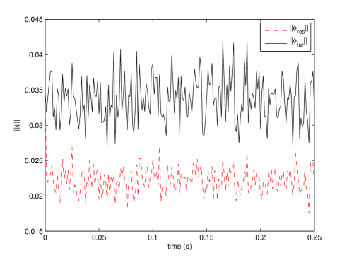
Figure 5: Time-evolution of $\|\phi_{\textnormal{tur}}\|_{L^{2}(\Omega)}$ (solid line) and $\|\phi_{\textnormal{res}}\|_{L^{2}(\Omega)}$ (dashed line)

Using Monte Carlo simulations, the ratio between temporal average of $\|\phi_{\textnormal{tur}}\|_{L^{2}(\Omega)}$ and $\|\phi_{\textnormal{res}}\|_{L^{2}(\Omega)}$ is near to 1.91 which represents a phase distortion attenuation of the reflected wavefront of $48\%$. In addition one should recall that this result does not take into account the tip/tilt correction. Even if these results are of the same order of magnitude as those presented in [9], which cannot be considered as completely satisfactory when considering usual results on real experiments, they clearly demonstrate the feasibility of the proposed approach. The possible degradation of such a performance induced by the delay in the loop and the discretization of the control law for implementation purpose could darken the picture. It must be recalled that this apparent loss of performance is mainly due to the tuning of the trade-off between robustness and performance that is inherently encountered in closed-loop feedback design. Numerous improvements have still to be considered as presented in the next conclusion.

5 Conclusion

In this paper, a new framework to deal with the problem of adaptive optics is proposed. It is mainly based on an infinite-dimensional model of the deformable mirror associated with the definition of a standard model on which robust control techniques may be applied. The preliminary numerical experiments show a performance level comparable with the results of reference [9]. The main advantage of the approach suggested in this paper is that no interaction matrix is required to control the system. We do not pretend to outperform already existing AO systems but rather to pave the way for future major improvements in terms of robustness and efficiency of the proposed control strategies. The authors are planing to take into account a model for the Shack-Hartmann wavefront sensor including a time delay associated with processing measurements. This will be covered in a next study.

References

- [1] F. Rodier, Adaptive optics in Astronomy, Cambridge University Press, 1999.
- [2] H.-F. Raynaud, C. Kulcsár, C. Petit, J.-M. Conan, P. Viaris de Lesegno, Optimal control, observers and integrators in adaptive optics, Optics express, Vol. 14, No. 17, 2006.
- [3] B.W. Frazier, R.K. Tyson, M. Smith and J. Roche, Theory and operation of a robust controller for a compact adaptive optics system, Opt. Eng. (2004) 43 (12), 2912-2920.
- [4] L. Baudouin, C. Prieur and D. Arzelier Robust control of a bimorph mirror for adaptive optics system, 17th International Symposium on Mathematical Theory of Networks and Systems (MTNS 2006).
- [5] D.W. Miller and S.C.O. Grocott, Robust control of the multiple mirror telescope adaptive secondary mirror, Opt. Eng., (1999) 38 (8), 1276-1287.
- [6] J.-M. Conan, G. Rousset et P.Y Madec Wavefront temporal spectra in high resolution imaging through turbulence, J. Opt. Soc. Am. A, Vol. 12, No. 7(1995).
- [7] M. Lenczner and C. Prieur, Asymptotic model of an active mirror, 13th IFAC Workshop on Control Appli. of Optimization, Cachan, France, 2006. http://www.laas.fr/cprieur/Papers/tomo2.pdf
- [8] B. Van Keulen, -control with measurement-feedback for linear infinite-dimensional systems J. Math. Syst. Estim. Control 3 (1993), 4, 373-411.
- [9] R. Paschall and D. Anderson Linear quadratic Gausian control of a deformable mirror adaptive optics system with time-delayed measurments, Applied optics, Vol.32 No 31, 1993.
- [10] S. Skogestad and I. Postlethwaite Multivariable Feedback Control - Analysis and design, Wiley, 1996 (2005).
- [11] J. F. Nye, Physical Properties of Crystals, Their Representation by Tensors and Matrices, Oxford University Press, 1985.
- [12] R. Noll, Zernike polynomials and atmospheric turbulence, The Optical Society of America, Vol 66 No 3, 1976.
- [13] C. Hogge and R. Butts Frequency spectra for the geometric representation of wavefront distortions due to atmospheric turbulence, IEEE transactions on antennas and propagation, 1976.
- [14] A. Bensoussan and P. Bernhard On the standard problem of -optimal control for infinite-dimensional systems, Identification and control in systems governed by partial differential equations , SIAM, Philadelphia, PA (1993) 117-140.
- [15] R. Curtain A. M. Peters and B. Van Keulen, -control with state-feedback: the infinite-dimensional case, J. Math. Syst. Estim. Control, 3 (1993), 1, 1-39.
- [16] J.-L. Lions and G. Duvaut, Les inéquations en Mécanique et en Physique, Dunod, 1972.
- [17] M. Pazy Semigroups of linear operators and applications to partial differential equations, Applied Mathematical Sciences, 44 Springer-Verlag, New York, 1983.
- [18] Z.-H. Luo, B.-Z. Guo and O. Morgul Stability and stabilization of infinite dimensional systems with applications, Communications and Control Engineering Series. Springer-Verlag, London, 1999.
- [19] M. Amabili, A. Pasqualini and G. Dalpiaz Natural frequencies and modes of free-edge circular plates vibrating in vacuum or in contact with liquid J. Sound Vibration 188 (1995), no. 5, 685-699.
- [20] R.D. Blevins, Formulas for natural frequency and mode shape, Kriger, 1979.