Optimal estimation of entanglement

Abstract

Entanglement does not correspond to any observable and its evaluation always corresponds to an estimation procedure where the amount of entanglement is inferred from the measurements of one or more proper observables. Here we address optimal estimation of entanglement in the framework of local quantum estimation theory and derive the optimal observable in terms of the symmetric logarithmic derivative. We evaluate the quantum Fisher information and, in turn, the ultimate bound to precision for several families of bipartite states, either for qubits or continuous variable systems, and for different measures of entanglement. We found that for discrete variables, entanglement may be efficiently estimated when it is large, whereas the estimation of weakly entangled states is an inherently inefficient procedure. For continuous variable Gaussian systems the effectiveness of entanglement estimation strongly depends on the chosen entanglement measure. Our analysis makes an important point of principle and may be relevant in the design of quantum information protocols based on the entanglement content of quantum states.

I Introduction

Entanglement is perhaps the most distinctive feature of quantum mechanics, and definitely the most relevant resource for quantum information processing EntR . Indeed, quantification of entanglement and schemes for its measurement have been the subject of extensive efforts in the last decade Aud06 ; Che03 ; Eis07 ; Guh04 ; Guh07 ; Sun07 ; Lou06 ; Wal06 ; Ren04 ; Nav08 ; Hor03 ; Aci00 ; Hor02 ; Dur01 ; Bar03 ; Guh03 ; Dar03 ; Pla02 ; Pit03 . Indeed, the entanglement content of a quantum state is a crucial piece of information in the design of quantum information protocols, and a question naturally arises on whether quantum mechanics itself poses limits to the precision of its determination. As a matter of fact, any quantitative measure of entanglement corresponds to a nonlinear function of the density operator and thus cannot be associated to a quantum observable. As a consequence, any procedure aimed to evaluate the amount of entanglement of a quantum state is ultimately a parameter estimation problem, where the value of entanglement is indirectly inferred from the measurement of one or more proper observables. An optimization problem thus naturally arises, which may be properly addressed in the framework of quantum estimation theory (QET) QET , which provides analytical tools to find the optimal measurement according to some given criterion.

Our aim is indeed to evaluate the ultimate bounds to precision posed by quantum mechanics, i.e the smallest value of the entanglement that can be discriminated, and to determine the optimal measurements achieving those bounds. Being entanglement an intrinsic property of quantum states we adopt local quantum estimation theory, where the optimal estimators are those maximizing the Fisher information Hel67 ; BC94 ; BC96 and in turn minimizing the variance at fixed value of entanglement. Local QET provides any family of quantum states with a geometric structure based on distinguishability and accounts for the optimal measurement that can be performed on the quantum system as well as the optimal data processing of the outcomes of the measurement.

Local QET has been applied to the estimation of quantum optical phase Mon06 as well as to estimation problems involving non unitary processes in open quantum systems Sar06 , either in finite dimensional systems Hot06 or continuous variable ones Mon07 . This includes the optimal estimation of the noise parameter of depolarizing Fuj01 or amplitude-damping Zhe06 ; Mon07 channels. Recently, the geometric structure induced by the Fisher information itself has been exploited to give a quantitative operational interpretation for multipartite entanglement Boi08 and to assess quantum criticality as a resource for quantum estimation ZP07 .

In this paper we systematically apply local QET to the problem of efficiently estimate the amount of entanglement of a quantum state. We consider several families of bipartite states, either for qubits or Gaussian states, and evaluate the symmetric logarithmic derivative to estimate entanglement through different measures, e.g. negativity or linear entropy. Then we explicitly calculate the quantum Fisher information and derive the ultimate bounds to the precision of estimation. Overall, we found that, both for qubits and Gaussian states, entanglement may be efficiently estimated when it is large. On the other hand the estimation of a small amount of entanglement for qubits is an inherently inefficient procedure, i.e the signal-to-noise ratio is vanishing for vanishing entanglement, whereas for Gaussian states it depends on the chosen measure of entanglement. We also found that the presence of other free parameters besides entanglement does not generally influence the estimation precision, thus preventing the possibility of further optimizing the estimation procedure.

The paper is structured as follows: in the next Section we give some basic elements of quantum estimation theory and introduce the quantum signal-to-noise to assess the estimability of a parameter. In Section III we analyze the estimation of entanglement by means of negativity NVW and linear entropy for the family of pure two-qubit states as well as for two families of entangled mixtures. In Section IV we address a family of PPT bound-entangled states HorodPPT for two-qutrit systems as an example of states with an inherently small amount of entanglement. In Section V we address entanglement estimation for Gaussian states, either pure states (twin-beams) or entangled mixtures. Section VI closes the paper with some concluding remarks.

II Quantum estimation theory

In an estimation problem one tries to infer the value the of a parameter $\lambda$ by measuring a different quantity $X$, which is somehow related to $\lambda$. An estimator $\hat{\lambda}\equiv\lambda(x_{1},x_{2},..)$ for $\lambda$ is a real function of the outcomes of measurement. The Cramer-Rao theorem Cra46 establishes a lower bound for the variance ${\mathrm{Var}}(\lambda)$ of any unbiased estimator

$${\mathrm{Var}}(\lambda)\geq\frac{1}{MF(\lambda)}$$ (1)

in terms of the number of measurements $M$ and the so-called Fisher Information (FI)

$$F(\lambda) =\sum_{x}p(x|\lambda)\,[\partial_{\lambda}\ln p(x|\lambda)]^{2}=\sum_{x}\frac{[\partial_{\lambda}p(x|\lambda)]^{2}}{p(x|\lambda)},$$ (2)

where $p(x|\lambda)$ denotes the conditional probability of obtaining the value $x$ when the parameter has the value $\lambda$.

In quantum mechanics, according to the Born rule we have $p(x|\lambda)=\hbox{Tr}[E_{x}\varrho_{\lambda}]$ where $\left\{E_{x}\right\}$ are the elements of a positive operator-valued measure (POVM) and $\varrho_{\lambda}$ is the density operator parametrized by the quantity we want to estimate. Introducing the Symmetric Logarithmic Derivative (SLD) $L_{\lambda}$ as the operator satisfying the equation

$$\frac{L_{\lambda}\varrho_{\lambda}+\varrho_{\lambda}L_{\lambda}}{2}=\frac{\partial\varrho_{\lambda}}{\partial\lambda}$$ (3)

we have that $\partial_{\lambda}p(x|\lambda)=\hbox{Tr}[\partial_{\lambda}\varrho_{\lambda}E_{x}]=\hbox{Re}(\hbox{Tr}[\varrho_{\lambda}L_{\lambda}E_{x}])$, and the Fisher Information in Eq. (2) may be rewritten as

$$F(\lambda)=\sum_{x}\frac{\hbox{Re}(\hbox{Tr}[\varrho_{\lambda}L_{\lambda}E_{x}])^{2}}{\hbox{Tr}[\varrho_{\lambda}E_{x}]}.$$ (4)

Starting from Eq. (4) one may prove that $F(\lambda)$ is upper bounded by the so-called Quantum Fisher Information (QFI) BC94 ; BC96

$$F(\lambda)\leq H(\lambda)\equiv\hbox{Tr}[\varrho_{\lambda}L_{\lambda}^{2}]\>,$$ (5)

and, in turn, that $\hbox{Var}(\lambda)\geq[MH(\lambda)]^{-1}$ represents the quantum version of the Cramer-Rao theorem, i.e. the ultimate bound to precision for any quantum measurement aimed to estimate the parameter $\lambda$. The SLD itself provides an optimal measurement, that is, using a measurement described by the projectors over the eigenbasis of $L_{\lambda}$ we saturate inequality (5).

Upon diagonalizing $\varrho_{\lambda}=\sum_{k}p_{k}|\psi_{k}\rangle\langle\psi_{k}|$ and using Eqs. (3) and (5) we obtain

$$L_{\lambda} =2\sum_{n,m}\frac{\langle\psi_{n}|\partial_{\lambda}\varrho_{\lambda}|\psi_{m}\rangle}{p_{n}+p_{m}}|\psi_{n}\rangle\langle\psi_{m}|$$ (6)

$$H(\lambda) =\sum_{n}\frac{(\partial_{\lambda}p_{n})^{2}}{p_{n}}+2\sum_{n,m}\frac{(p_{n}-p_{m})^{2}}{p_{n}+p_{m}}|\langle\psi_{n}|\partial_{\lambda}\psi_{m}\rangle|^{2}\,$$

which, for a family of pure states $\varrho_{\lambda}=|\psi_{\lambda}\rangle\langle\psi_{\lambda}|$ reduces to

$$L_{\lambda} =2\,\partial_{\lambda}|\psi_{\lambda}\rangle\langle\psi_{\lambda}|$$ (7)

$$H(\lambda) =4\left[\langle\partial_{\lambda}\psi_{\lambda}|\partial_{\lambda}\psi_{\lambda}\rangle+\langle\partial_{\lambda}\psi_{\lambda}|\psi_{\lambda}\rangle^{2}\right]\,.$$

When more than a parameter are involved we have quantum states $\varrho_{\Lambda}$ depending on a set of $N$ parameters $\Lambda=\{\lambda_{j}\}$, $j=1,\dots,N$. In this case the geometry of the estimation problem is contained in the QFI matrix, whose elements are defined as ${\boldsymbol{H}}(\Lambda)_{ij}=\frac{1}{2}\hbox{Tr}[\varrho_{\Lambda}\{L_{i},L_{j}\}]$ where $L_{i}$ is the SLD that corresponds to the parameter $\lambda_{i}$ and $\{A,B\}=AB+BA$ denotes anti-commutator. The explicit formula for the QI matrix reads as follows

$$H(\Lambda)_{ij}=\sum_{n}\frac{(\partial_{i}p_{n})(\partial_{j}p_{n})}{p_{n}}+\sum_{n,m}\frac{(p_{n}-p_{m})^{2}}{p_{n}+p_{m}}\times$$

$$\times(\langle\psi_{n}|\partial_{i}\psi_{m}\rangle\langle\partial_{j}\psi_{m}|\psi_{n}\rangle+\langle\psi_{n}|\partial_{j}\psi_{m}\rangle\langle\partial_{i}\psi_{m}|\psi_{n}\rangle)$$ (8)

The inverse of the Fisher matrix provides a lower bound ${\boldsymbol{\gamma}}\geq H^{-1}$, on the covariance matrix ${\boldsymbol{\gamma}}_{ij}=\langle\lambda_{i}\lambda_{j}\rangle-\langle\lambda_{i}\rangle\langle\lambda_{j}\rangle$ of global estimators of $\Lambda$, which is not generally achievable. On the other hand, the diagonal elements of the inverse Fisher matrix provide achievable bounds for the variances of single parameter estimators (at fixed value of the others)

$${\mathrm{Var}}(\lambda_{i})={\boldsymbol{\gamma}}_{ii}\geq({\boldsymbol{H}}^{-1})_{ii}.$$ (9)

Let us now suppose to reparametrize the family of quantum states with a new set of parameters $\tilde{\Lambda}=\{\tilde{\lambda}_{j}=\tilde{\lambda}_{j}(\Lambda)\}$. We have $\tilde{\partial}_{j}=\sum_{i}B_{ij}\partial_{i}$ with $B_{ij}=\partial\lambda_{i}/\partial\tilde{\lambda}_{j}$ and, in turn

$$\tilde{L}_{j} =\sum_{i}B_{ij}L_{i}$$

$$H(\tilde{\Lambda})_{ij} =\sum_{r,s}B_{ir}H(\Lambda)_{rs}B_{js}$$ (10)

i.e. $\widetilde{{\boldsymbol{H}}}={\boldsymbol{B}}{\boldsymbol{H}}{\boldsymbol{B}}^{T}$.

In the following we address the problem of finding the bounds to the estimation of the entanglement between the two subsystems $A,B$ of a family of bipartite quantum states. The general strategy will be to start from the expression of the family of states in terms of a given set of ”natural” parameters and then make a change of variable in order to write the state directly in terms of the chosen entanglement monotone $\lambda=\epsilon$. Once this is achieved, the results obtained hold, at every fixed value of the entanglement, for the whole orbit of states that can be obtained by acting on the given one with local unitary operators $U_{AB}\doteq U_{A}\otimes U_{B}$. Indeed, the latter, acting locally on the two subsystems $A$ and $B$, they do not change the entanglement of the state; furthermore they do not change the value of the QFI. This follows from the observation that, if a given $L_{\epsilon}$ is the solution of (3), the SLD that will correspond to $\tilde{\varrho}_{\epsilon}=U_{AB}\varrho_{\epsilon}U_{AB}^{\dagger}$ is given by $\tilde{L}_{\epsilon}=U_{AB}L_{E}U_{AB}^{\dagger}$ and, due to the cyclic property of the trace, $H(\epsilon)=\hbox{Tr}[\varrho_{\epsilon}L_{\epsilon}^{2}]=\hbox{Tr}[\tilde{\varrho}_{\epsilon}\tilde{L}_{\epsilon}^{2}]$.

We finally notice that in order to assess the estimability of a given parameter the relevant figure of merit is given by the signal-to-noise ratio

$$R(\lambda) =\frac{\lambda^{2}}{\mathrm{Var}(\lambda)}\leq Q(\lambda)=\lambda^{2}H(\lambda)\;,$$ (11)

rather than the variance itself. In particular the SNR of an estimator is relevant to assess its performances in estimating small values of the parameter. Eq. (11) shows that the SNR $R(\lambda)$ is bounded by the quantum signal-to-noise ratio (QSNR) $Q(\lambda)$ expressed in terms of the QFI. Upon taking into account repeated measurements we have that the number of measurements leading to a $99.9\%$ ($3\sigma$) confidence interval corresponds to a relative error

$$\delta^{2}=\frac{9\hbox{Var}(\lambda)}{M\lambda^{2}}=\frac{9}{M}\frac{1}{Q}(\lambda)=\frac{9}{M\lambda^{2}H(\lambda)}$$

Therefore, the number of measurements needed to achieve a $99.9\%$ confidence interval with a relative error $\delta$ scales as

$$M_{\delta}(\lambda)=\frac{9}{\delta^{2}}\frac{1}{Q(\lambda)}$$ (12)

In other words, a vanishing $Q(\lambda)$ implies a diverging number of measurements to achieve a given relative error, whereas for a finite $Q(\lambda)$ the number of measurements is determined by the desired level of precision. In order to have a non-vanishing $Q(\lambda)$ for small value of the parameter $\lambda$, the QFI should diverge at least as $H(\lambda)\sim\lambda^{-2}$ for vanishing $\lambda$. We notice that a similar quantity, namely $\lambda H(\lambda)$, has been used in to asses estimation strategy for the parameter of a qubit depolarizing channel Fuj03 .

III Two-qubit systems

In this section we analyze estimation of entanglement for families of two-qubit states and evaluate limits to precision using the formalism developed in the previous section. At first we address the set of pure states and then consider families of entangled mixtures. In both cases we consider different measures of entanglement.

III.1 Pure states

We start by considering the set of pure states of two qubits. Upon exploiting the Schmidt decomposition

$$|\Psi_{q}\rangle=\sqrt{q}|0\rangle_{A}|0\rangle_{B}+\sqrt{1-q}|1\rangle_{A}|1\rangle_{B}\>,$$ (13)

the whole family of pure states can be parametrized by a single parameter: the Schmidt coefficient $q$. Since for two-qubit pure states $q$ is itself an entanglement monotone, all measures of entanglement can be expressed as a monotone function $\epsilon=\epsilon(q)$. As a consequence, in order to determine the precision of estimation it suffices to evaluate the QFI $H(q)$ and then use the rule for repametrization in Eq. (10), i.e. $H(\epsilon)=H[q(\epsilon)][\partial_{\epsilon}q(\epsilon)]^{2}$. Since the states are pure, the SLD may be evaluated as $L_{q}=2\partial_{q}|\Psi_{q}\rangle\!\langle\Psi_{q}|$; the resulting Cramer-Rao bound and the QSNR read as follows

$${\mathrm{Var}}(q) \geq H(q)^{-1}=q(1-q)$$ (14)

$$Q(q) =\frac{q}{1-q}\stackrel{{\scriptstyle q\rightarrow 0}}{{\sim}}q\>.$$ (15)

$Q(q)$ vanishes for vanishing $q$, thus indicating that any estimator of the Schmidt coefficient $q$ becomes less and less precise for vanishing $q$. It is worth noting that the Schmidt coefficient $q$ coincides with the only independent eigenvalue of the reduced density matrix $\varrho_{A(B)}=\hbox{diag}\{q,1-q\}$, which is diagonal in the Schmidt basis. Therefore the QSNR in Eq. (15) also imposes bound to the determination of the eigenvalue of $\varrho_{A(B)}$. Indeed, the same bound could have been obtained by applying the estimation machinery directly to $\varrho_{A(B)}$.

Let us now consider two different measures of entanglement for pure two-qubit states, i.e the negativity $\epsilon_{\hbox{\tiny N}}$ NVW and the (normalized) linear entropy $\epsilon_{\hbox{\tiny L}}=2(1-\hbox{Tr}[\varrho_{A}^{2}])$. In terms of the Schmidt coefficient $q$ we have

$$\epsilon_{\hbox{\tiny N}}=\sqrt{\epsilon_{\hbox{\tiny L}}}=2\sqrt{q(1-q)}$$ (16)

We recall that the negativity is a good measure of entanglement for generic two-qubit states, i.e it is an entanglement monotone and it differs from zero iff the state is entangled, whereas the linear entropy is a good entanglement monotone only iff the state is pure. Upon expressing the Schmidt coefficient as $q=\frac{1}{2}(1-\sqrt{1-\epsilon_{\hbox{\tiny N}}^{2}})$ and using (10), we have $\mathrm{Var}(\epsilon_{\hbox{\tiny N}})\geq H(\epsilon_{\hbox{\tiny N}})^{-1}=1-\epsilon_{\hbox{\tiny N}}^{2}$, $\mathrm{Var}(\epsilon_{\hbox{\tiny N}})\geq H(\epsilon_{\hbox{\tiny L}})=4\epsilon_{\hbox{\tiny L}}(1-\epsilon_{\hbox{\tiny L}})$ and, in turn,

$$Q(\epsilon_{\hbox{\tiny N}}) =\frac{\epsilon_{\hbox{\tiny N}}^{2}}{1-\epsilon_{\hbox{\tiny N}}^{2}}\stackrel{{\scriptstyle\epsilon_{\hbox{\tiny N}}\rightarrow 0}}{{\sim}}\epsilon_{\hbox{\tiny N}}^{2}$$ (17)

$$Q(\epsilon_{\hbox{\tiny L}}) =\frac{\epsilon_{\hbox{\tiny L}}}{4(1-\epsilon_{\hbox{\tiny L}})}\stackrel{{\scriptstyle\epsilon_{\hbox{\tiny L}}\rightarrow 0}}{{\sim}}\epsilon_{\hbox{\tiny L}}/4\>.$$ (18)

The optimal estimator for the Schmidt coefficient has a variance ${\mathrm{Var}}(q)$ which is minimum for $q=0,1$ (product state) and maximum for $q=1/2$ (Bell state) whereas for the two entanglement measure we have that ${\mathrm{Var}}(\epsilon_{\hbox{\tiny N}})$ is monotonically decreasing with $\epsilon_{\hbox{\tiny N}}$; ${\mathrm{Var}}(\epsilon_{\hbox{\tiny L}})$ is minimum when the state is either in a product form ($\epsilon_{\hbox{\tiny L}}=0$) or is maximally entangled ($\epsilon_{\hbox{\tiny L}}=1$) and is maximum in the ”intermediate” case ($\epsilon_{\hbox{\tiny L}}=1/2$). Despite the variances behave quite differently we have the same qualitative behavior of the quantum signal-to-noise ratios and of the number of measurement necessary at fixed relative error $M_{\delta}$. Indeed, in all cases the QSNR is an increasing function of the parameter and it diverges when the latter takes its maximum value ($q=1$, $\epsilon_{\hbox{\tiny N}}=\epsilon_{\hbox{\tiny L}}=1$); $M_{\delta}(\epsilon)$ diverges for $\epsilon=\epsilon_{\hbox{\tiny N}}=\epsilon_{\hbox{\tiny L}}=0$ and then decreases monotonically, going to zero for the maximum value of entanglement $\epsilon=\epsilon_{\hbox{\tiny N}}=\epsilon_{\hbox{\tiny L}}=1$ . Moreover for vanishing entanglement the QNSR of the linear entropy estimator is vanishing slower than the corresponding quantity for the negativity. We conclude that the linear entropy is a more efficient entanglement estimator though, being the QSNR vanishing, the estimation is anyway inherently inefficient.

The above result can obviously generalized to the case of systems composed by a qubit and an $N$-level system; indeed only two of the dimensions of the latter can be used to express the state: the reduced density matrices of both subsystems have only two non zero eigenvalues.

III.2 Entangled mixtures

We now consider few families of mixed entangled states with different properties and show that they exhibit a common behavior concerning estimation of entanglement. The first family is described by the set of density matrices

$$\varrho=U(q)\nu_{p}U^{\dagger}(q)$$ (19)

where

$$\nu_{p} =p|0,0\rangle\!\langle 0,0|+(1-p)|1,1\rangle\!\langle 1,1|$$

$$U(q) =\exp\{i\,\hbox{arcos}\,q\,\sigma_{x}\otimes\sigma_{x}\}\,.$$

These states depend on two parameters $(q,p)$ and are obtained via the action of the entangling operator $U(q)$ on the classically correlated state $\nu_{p}$. Upon varying the parameter $p$ we may control the purity $\mu(p)=1-2p(1-p)$ of the state, while varying $q$ we tune the amount of entanglement. The QFI matrix is diagonal with elements:

$${\boldsymbol{H}}(p,q)=\hbox{diag}\left(\frac{1}{p(1-p)},\frac{(1-2p)^{2}}{q(1-q)}\right)$$ (20)

The negativity of the state (19) is given by the unique negative eigenvalue of the partially transposed state $\varrho^{T_{A}}$:

$$\epsilon_{\hbox{\tiny N}}=2\sqrt{q(1-q)}(1-2p)$$ (21)

Upon inverting the above relation and the one for the purity, we reparametrize the set of states in terms of the new parameter $(p,q)\rightarrow(\mu,\epsilon_{\hbox{\tiny N}})$. The transfer matrix is given by

$${\boldsymbol{B}}=\left(\begin{array}[]{cc}-\frac{1}{2\sqrt{2\mu-1}}&\frac{\epsilon_{\hbox{\tiny N}}^{2}}{2\sqrt{(2\mu-1)^{2}(2\mu-1-\epsilon_{\hbox{\tiny N}}^{2})}}\\ 0&\frac{\epsilon_{\hbox{\tiny N}}}{2\sqrt{(2\mu-1)(2\mu-1-\epsilon_{\hbox{\tiny N}}^{2})}}\end{array}\right)$$ (22)

and the inverse QFI matrix:

$${\boldsymbol{H}}(\mu,\epsilon_{\hbox{\tiny N}})^{-1}=\left(\begin{array}[]{cc}-4\mu^{2}+6\mu-2&2\epsilon_{\hbox{\tiny N}}(1-\mu)\\ 2\epsilon_{\hbox{\tiny N}}(1-\mu)&1-\epsilon_{\hbox{\tiny N}}^{2}\end{array}\right)$$ (23)

The corresponding bound on the variance is thus given by:

$${\mathrm{Var}}(\epsilon_{\hbox{\tiny N}})\geq\left({\boldsymbol{H}}(\mu,\epsilon_{\hbox{\tiny N}})^{-1}\right)_{22}=1-\epsilon_{\hbox{\tiny N}}^{2}\,$$ (24)

which represents the bound to the precision of any entanglement (negativity) estimation procedure performed at fixed purity $\mu$. The result in Eq. (24) is independent on the purity, no optimization procedure may be pursued, and it coincides with the bound obtained and discussed in the previous subsection for pure states.

Let us now consider the family of Werner-like states

$$\varrho_{pq}=\frac{1-p}{4}\openone\otimes\openone+p|\Psi_{q}\rangle\!\langle\Psi_{q}|$$ (25)

obtained by depolarizing an entangled state $|\Psi_{q}\rangle$ of the form given in Eq. (13). This set of states depends on two parameters $p,q$. As in the previous example upon varying the parameter $p$ we may control the purity $\mu(p)=(1+3p^{2})/4$ of the state, while the amount of entanglement depends on both parameters. The eigenvalues of $\varrho_{pq}$ depends only on $p$ whereas the eigenvectors depends only on $q$. The QFI matrix is thus given by the diagonal form

$${\boldsymbol{H}}(p,q)=\mbox{diag}\left\{\frac{3}{1+(2-3p)p},\,\,\frac{p^{2}}{q(1-q)(1+p)}\right\}\,$$ (26)

and the inverses of the diagonal elements correspond to the ultimate bounds to ${\mathrm{Var}}(p)$ and ${\mathrm{Var}}(q)$ of any estimator of $p$ and $q$, either at fixed value of the other parameter or in a joint estimation procedure. Entanglement of Werner states may be evaluated in terms of negativity,

$$\epsilon_{\hbox{\tiny N}}=\max\left\{0,\frac{1}{2}\left[p\left((1+4\sqrt{q(q-1)}\right)-1\right]\right\}\>,$$ (27)

which implies that Werner states are entangled for $(1>p>[1+4q(1-q)]^{-1}$. Upon inverting Eq. (27) for $p$ or $q$ we may parametrize the Werner states using $(\epsilon_{\hbox{\tiny N}},q)$ or $(p,\epsilon_{\hbox{\tiny N}})$ and evaluate the QFI matrices $H(\epsilon_{\hbox{\tiny N}},q)$ and $H(p,\epsilon_{\hbox{\tiny N}})$, their inverses and, in turn, the corresponding bounds to the precision of entanglement (negativity) estimation. The main results are that the ultimate bounds to the variance, and thus to the QSNR depend very slightly on the other free parameter ($q$ or $p$). In other words, estimation procedures performed at fixed value of $p$ or $q$ respectively shows different precision, but the differences are negligible in the whole range of variations of the parameters. We do not report here the analytic expression of $Q(\epsilon_{\hbox{\tiny N}})$ at fixed $p$ or $q$ which is quite cumbersome. Rather, we show the behavior of $Q(\epsilon_{\hbox{\tiny N}})$ in Fig. 1. On the left we show the QSNR $Q_{q=0.5}(\epsilon_{\hbox{\tiny N}})$ for $q=0.5$, whereas on the right we show the ratio $Q_{p}(\epsilon_{\hbox{\tiny N}})/Q_{q=0.5}(\epsilon_{\hbox{\tiny N}})$ for different value of $p$ (a similar behavior may be observed upon varying $q$). As it is apparent from the main panel the QSNR is a growing function of $\epsilon_{\hbox{\tiny N}}$, vanishes for vanishing negativity and diverges for maximally entangled states $\epsilon_{\hbox{\tiny N}}=1$. The inset shows that there is almost no dependence on the actual value of $p$ and $q$ respectively and this prevents any possible optimization of the estimation procedure. For small $\epsilon_{\hbox{\tiny N}}$ we have $Q(\epsilon_{\hbox{\tiny N}})\simeq f(q)\epsilon_{\hbox{\tiny N}}^{2}$ and $Q(\epsilon_{\hbox{\tiny N}})\simeq g(p)\epsilon_{\hbox{\tiny N}}^{2}$ respectively, where both the functions $f(q)\simeq 1$ and $g(p)\simeq 1$ are again very close to unit value for the whole ranges of variation of $q$ and $p$.

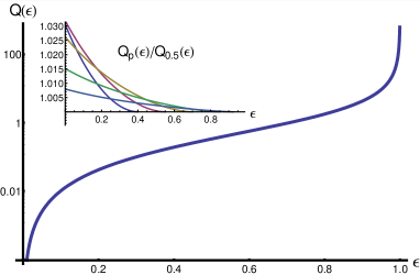
Figure 1: Quantum signal-to-noise ratio for the estimation of entanglement (negativity) of a two-qubit Werner state as a function of the negativity at fixed $q=0.5$. The inset shows the ratio $Q_{p}(\epsilon_{\hbox{\tiny N}})/Q_{q=0.5}(\epsilon_{\hbox{\tiny N}})$ for different value of $p$.

In all the cases we have considered, the QSNR is small for the most part of entanglement range and starts growing only for highly entangled states. In other words, estimation of entanglement is, on average, an inefficient procedure.

IV Two-qutrit bound entangled states

In the previous section we have seen how the estimation of entanglement, as measured by negativity is a fairly inefficient procedure for weakly entangled states. Here we want to test how the QFI and the related bounds behave when one considers states that have inherently small amount of entanglement. A paradigmatic examples of such states are the so called bound entangled states, which exhibit non-classical correlations even if they satisfy the separability criterion based on partial transposition of the density matrix HorodPPT ; PeresSep ; HorodSep . The first example of bound entangled states is given by the following family of two spin-1 states HorodPPT

$$\varrho_{a} = \frac{a}{1+8a}\big{(}|\downarrow 0\rangle\langle\downarrow 0|+|\downarrow\uparrow\rangle\langle\downarrow\uparrow|+|0\downarrow\rangle\langle 0\downarrow|$$ (28)

$$+ |0\uparrow\rangle\langle 0\uparrow|+|\uparrow 0\rangle\langle\uparrow 0|\big{)}+\frac{3a}{1+8a}|E\rangle\langle E|$$

$$+ \frac{1}{1+8a}|\Pi\rangle\langle\Pi|$$

where

$$|E\rangle =\frac{1}{\sqrt{3}}\left(|\downarrow\downarrow\rangle+|00\rangle+|\uparrow\uparrow\rangle\right)$$

$$|\Pi\rangle =\sqrt{\frac{1+a}{2}}|\uparrow\downarrow\rangle+\sqrt{\frac{1-a}{2}}|\uparrow\uparrow\rangle.$$

Since for all values of the parameter $a$ $\;\varrho_{a}$ has a positive partial transpose (PPT), negativity cannot be used as a measure of the quantum correlations present in state. In order to estimate the entanglement we will use the scheme proposed in HoffmanLUR ; HoffmanLURPPT . The latter is based on the following considerations. Given the sets of $n$ non-commuting operators $\{A_{i}\}$ and $\{B_{i}\}$ acting locally on the subsystem A and B respectively one has a lower bound for the sum of the local uncertainties relations (LUR):

$$\sum_{i}\delta A_{i}^{2}>U_{A}\mbox{ and }\sum_{i}\delta B_{i}^{2}>U_{B}$$ (29)

where $\delta O_{i}^{2}=\left\langle O_{i}^{2}\right\rangle-\left\langle O_{i}\right\rangle^{2}$ is the variance of the operator $O_{i}$. Since for all separable states on has that $\sum_{i}\delta(A_{i}+B_{i})^{2}>U_{A}+U_{B}$, the latter inequality set a necessary condition for a state to be entangled. The relative violation of the inequality defined as

$$\epsilon_{\hbox{\tiny U}}=1-\frac{\sum_{i}\delta(A_{i}+B_{i})^{2}}{U_{A}+U_{B}}$$ (30)

can then be used as a measure of the quantum correlations present in the given state. The violation is necessary condition for the presence of the entanglement, thus, in order to effectively have and maximize such violation one can judiciously choose and optimize the choice of the sets $\{A_{i}\}$ and $\{B_{i}\}$. The result of a possible optimization for the state $\varrho_{a}$ is given in HoffmanLURPPT and the corresponding relative violation depends on the parameter $a$ and is given by:

$$\epsilon_{\hbox{\tiny U}}(\varrho_{a})=\frac{3a^{2}(1-a)}{4(2+a)(1+8a)^{2}}$$ (31)

The latter expression can be used to parameterize the state $\varrho_{a}$ in terms of $\epsilon_{\hbox{\tiny U}}(\varrho_{a})$ and then apply the QFI machinery in order to obtain the desired bound on the estimation of relative violation of the LUR. The results are shown in Fig. 2. We first note that the relative violation of the LUR is small, i.e $\epsilon_{\hbox{\tiny U}}(\varrho_{a})\in[0,2/1125]$. Nonetheless, the number of measurements $M_{\delta}(\epsilon_{\hbox{\tiny U}})$ is of the same order of those needed in the qubit case $M_{\delta}(\epsilon_{\hbox{\tiny N}})$ in similar conditions, and thus the overall efficiency of the estimation process is comparable for most part of the entanglement range. Finally, we notice that also for this family of qutrits the number of measurements $M_{\delta}(\epsilon_{\hbox{\tiny U}})$ diverges for vanishing entanglement.

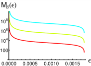
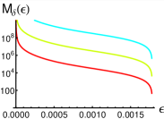
Figure 2: Number of measurement $M_{\delta}(\epsilon_{\hbox{\tiny U}})$ needed to achieve a given relative error $\delta=10^{-1}$ (red), $\delta=10^{-2}$ (green), $\delta=10^{-3}$ (blue) in the the estimation of LUR entanglement measure $\epsilon_{\hbox{\tiny U}}$ of PPT state $\varrho_{a}$ in Eq.(28). Left: $a\in[0,4/13]$, Right: $a\in[4/13,1]$

V Gaussian states

In this section analyze continuous variable systems and derive the bounds for the estimation of entanglement of two-mode Gaussian states GaussiansAOP . After a brief introduction we consider both pure states, i.e. twin-beam and the family of mixed states represented by squeezed thermal states (STS). Different measures of entanglement will be considered.

The characteristic function of the state $\varrho$ is defined as $\chi[\varrho]({\bf\Gamma})=\hbox{Tr}\left[\varrho\,D(\Gamma)\right]$ where $D(\Gamma)=\exp{\left[i\textbf{R}^{T}{\bf\Omega}{\bf\Gamma}\right]}$ is the displacement operator, defined in terms of the symplectic matrix

$${\bf\Omega}=\bigoplus_{k=1}^{n}\left(\begin{array}[]{cc}0&1\\ -1&0\\ \end{array}\right)_{n}$$ (32)

and the vector $\textbf{R}^{T}=(q_{1},p_{1},\cdots,q_{n},p_{n})$ of canonical operators. ${\bf\Gamma}^{T}=(a_{1},b_{1},\cdots,a_{n},b_{n})$ denotes the Cartesian coordinates and we have $\left[R_{k},R_{h}\right]=i{\bf\Omega}_{kh}$. Two-mode Gaussian state are those with a characteristic function of the form

$$\chi[\varrho]({\bf\Gamma})=\exp{\left(-\frac{1}{2}{\bf\Gamma}^{T}{\bf\sigma}{\bf\Gamma}+i{\bf\Gamma}^{T}{\bf\overline{X}}\right)}$$ (33)

where

$${\bf\sigma}_{kh}=\frac{1}{2}\langle\{R_{k},R_{h}\}\rangle-\langle R_{k}\rangle\langle R_{h}\rangle$$ (34)

is the covariance matrix of the second moments and ${\bf\overline{X}}$ denotes mean values. The second term in the exponential does not contain any information about entanglement, and can be set to zero via local operation. The covariance matrix completely characterize the state and by means of local symplectic transformations can be transformed into the standard block form : ${\sigma}=\left(\begin{array}[]{cc}A&C\\ C&B\end{array}\right)$ where $A=\hbox{Diag}(a,a)$, $B=\hbox{Diag}(b,b)$, and $C=\hbox{Diag}(c_{+},c_{-})$. For two-mode Gaussian states PPT condition is necessary and sufficient for separability and thus the entanglement properties of the state are encoded in the least symplectic eigenvalue GaussianCrit

$$\tilde{d}_{-}=\sqrt{(a-c_{+})(a+c_{-})}$$ (35)

where the symplectic spectrum of ${\bf\sigma}^{T_{A}}$ can be evaluated by finding the eigenvalues of ${\bf\Omega^{-1}}{\bf\sigma}^{T_{A}}.$ In this framework the PPT criterion can be cast in term of the smallest symplectic eigenvalue i.e., $\varrho$ is separable iff $\tilde{d}_{-}\geq 1/2$. Indeed, $\tilde{d}_{-}$ is itself an entanglement monotone. Furthermore, all the different entanglement measures for symmetric Gaussian states that have been proposed NVW ; EoFGiedke ; EntBuresMarian1 turns out to be a monotone function of the smallest symplectic eigenvalue. Since we are interested in the estimation of entanglement, we may first study the estimation of the symplectic eigenvalue $\tilde{d}_{-}$ and then use repametrization in order to asses the performances of other entanglement monotones. In particular, we will focus on the following measures:

$$\epsilon_{\hbox{\tiny N}}(\tilde{d}_{-}) =\max{\{0,-\ln{2}\tilde{d}_{-}\}}$$ (36)

$$\epsilon_{\hbox{\tiny L}}(\tilde{d}_{-}) =1-\frac{4\tilde{d}_{-}}{1+4\tilde{d}_{-}^{2}}$$ (37)

$$\epsilon_{\hbox{\tiny S}}(\tilde{d}_{-}) =1-2\tilde{d}$$ (38)

$$\epsilon_{\hbox{\tiny B}}(\tilde{d}_{-}) =\frac{(1-\sqrt{2\tilde{d}})^{2}}{1+2\tilde{d}}.$$ (39)

where the expressions for the linear entropy $\epsilon_{\hbox{\tiny L}}$ has been obtained in the pure state case. In particular $\epsilon_{\hbox{\tiny L}}$ and the logarithmic negativity $\epsilon_{\hbox{\tiny N}}$ will be used for pure states, whereas the Bures distance-based measure $\epsilon_{\hbox{\tiny B}}$ and $\epsilon_{\hbox{\tiny S}}$ EntBuresMarian1 will be used for mixed states. Notice that $\epsilon_{\hbox{\tiny B}}$ is a good measure of entanglement just for symmetric two-mode Gaussian states and that Eq. (38) has been obtained for this particular class of states. In order to evaluate the QFI, one has first to determine the actual expression of $\tilde{d}_{-}$. Then, one expresses the elements of the covariance matrix in terms of the chosen entanglement monotone and proceeds with the repametrization rules described in Section II.

V.1 Pure states

Here we address estimation of the entanglement of pure two modes Gaussian states, i.e. twin-beam. These are defined by the following relations between the elements of the covariance matrix: $a=b$ i.e., the states are symmetric and $c_{+}=-c_{-}=\sqrt{a^{2}-1/4}$. The states can thus be described by the single parameter $a$ or, by inverting $\tilde{d}_{-}=a-\sqrt{a^{2}-1/4}$ they can be completely described by their entanglement content. For Gaussian states the evaluation of the SLD and the QFI, besides the use of Eqs. (6), may be pursued using phase-space techniques. In fact, for pure states we have $L_{\epsilon}=2\partial_{\epsilon}\varrho_{\epsilon}$ and this allows to directly evaluate the characteristic function of the SLD as follows

$$\chi[L_{\epsilon}](\bf\Gamma)=2\partial_{\epsilon}\chi[\varrho_{\epsilon}]=-{\bf\Gamma}^{T}\partial_{\epsilon}\sigma_{\epsilon}{\bf\Gamma}\ \chi[\varrho_{\epsilon}]\>.$$ (40)

where ${\bf\Gamma}^{T}=({\bf\Gamma_{1}}^{T},{\bf\Gamma_{2}}^{T})$. The corresponding QFI $H(\epsilon)=\mbox{Tr}[\varrho\,L_{\epsilon}^{2}]$ is given by

$$H(\epsilon) = \int\!\!\int\frac{d^{2}{\bf\Gamma}_{1}}{2\pi}\frac{d^{2}{\bf\Gamma}_{2}}{2\pi}\,\mathcal{I}\left(\epsilon,{\bf\Gamma}_{1},{\bf\Gamma}_{2}\right)$$ (41)

where the integrand function reads as follows

$$\mathcal{I} = \chi[L_{\epsilon}]({\bf\Gamma}_{1})\chi[L_{\epsilon}]({\bf\Gamma}_{2})\mbox{ Tr }[\varrho D^{\dagger}({\bf\Gamma}_{1})D^{\dagger}({\bf\Gamma}_{2})]$$ (42)

We now use the relations $D[{\bf\Gamma}]^{\dagger}=D[-{\bf\Gamma}]$ and $D({\bf\Gamma}_{1})D({\bf\Gamma}_{2})=D({\bf\Gamma}_{1}+{\bf\Gamma}_{2})g({\bf\Gamma}_{1},{\bf\Gamma}_{2})$ and we rewrite (42) as

$$\mathcal{I} = \left({\bf\Gamma}_{1}^{T}\partial_{\epsilon}\sigma_{\epsilon}{\bf\Gamma}_{1}\right)\left({\bf\Gamma}_{2}^{T}\partial_{\epsilon}\sigma_{\epsilon}{\bf\Gamma}_{2}\right)\cdot$$ (43)

$$\chi_{\varrho_{\epsilon}}({\bf\Gamma}_{1})\chi_{\varrho_{\epsilon}}({\bf\Gamma}_{2})\chi_{\varrho_{\epsilon}:}(-{\bf\Gamma}_{1}-{\bf\Gamma}_{2})g({\bf\Gamma}_{1},{\bf\Gamma}_{2})$$

$$= \left({\bf\Gamma}^{T}{\bf\Sigma_{1}}{\bf\Gamma}\right)\ \left({\bf\Gamma}^{T}{\bf\Sigma_{2}}{\bf\Gamma}\right)\ \exp{\left(-\frac{1}{2}{\bf\Gamma}^{T}{\bf\Delta}{\bf\Gamma}\right)}$$

where we have introduced the matrices:

$${\bf\Sigma}=\left(\begin{array}[]{cc}2\sigma&\sigma\\ \sigma&2\sigma\end{array}\right),{\bf\Sigma_{1}}=\left(\begin{array}[]{cc}\partial_{\epsilon}\sigma&0\\ 0&0\end{array}\right),{\bf\Sigma_{2}}=\left(\begin{array}[]{cc}0&0\\ 0&\partial_{\epsilon}\sigma\end{array}\right)$$

and where $\Delta={\bf\Sigma}+i\Upsilon$, with $\Upsilon=\frac{1}{2}\,\sigma_{y}\otimes{\mathbbm{I}}\otimes\sigma_{y}$ in terms of Pauli matrices. The result of the integration QFI is a function of $\epsilon,\partial_{\epsilon}\sigma_{\epsilon}$ and can be expressed in various ways depending on the entanglement monotone that one chooses to estimate. By setting $a=\frac{1}{2}\cosh\epsilon_{\hbox{\tiny N}}$ in the covariance matrix, one can use the logarithmic negativity $\epsilon_{\hbox{\tiny N}}$. In this case one finds that the QFI is independent on the entanglement content of the state.

If one uses directly the symplectic eigenvalue $\tilde{d}_{-}$ the QFI now depends on the entanglement monotone:

$$H(\tilde{d}_{-})=\tilde{d}_{-}^{-2}$$ (44)

and the minimal variance in the estimation can be obtained in the limit of infinite entanglement i.e., $\tilde{d}_{-}=0$. Moreover we observe that, while for the logarithmic negativity one sees that the QSNR $Q(\epsilon_{\hbox{\tiny N}})$ is simply proportional to $\epsilon_{\hbox{\tiny N}}^{2}$, if we consider the least symplectic eigenvalue we have $Q(\tilde{d}_{-})=1$ over the whole range of variation, i.e. the estimation procedure can be done efficiently either for highly entangled states and weakly entangled ones.

As a matter of fact, twin-beam may be also written in the Fock basis as $|\Psi\rangle=\sum_{n}f_{n}|n\rangle|n\rangle$ where, in terms of the log-negativity or the linear entropy one may write

$$f_{n}=\sqrt{2\frac{(\cosh\epsilon_{\hbox{\tiny N}}-1)^{n}}{(\cosh\epsilon_{\hbox{\tiny N}}+1)^{1+n)}}}\>=\sqrt{2\frac{\epsilon_{\hbox{\tiny L}}^{n}(1-\epsilon_{\hbox{\tiny L}})}{(2-\epsilon_{\hbox{\tiny L}})^{1+n}}}\,.$$ (45)

Using this representation we may directly exploit Eqs. (7): for a generic parameter $x$ and $f_{n}(x)\in\mathbb{R}$ we have $\langle\Psi|\partial_{x}\Psi\rangle=0$ and thus

$$H(x)=\langle\partial_{x}\Psi|\partial_{x}\Psi\rangle=\sum_{n}(\partial_{x}f_{n}(x))^{2}\>.$$ (46)

Using the above equation one recover the result for the log-negativity and may evaluate the QFI in terms of the linear entropy obtaining

$$H(\epsilon_{\hbox{\tiny L}})=\left(4(2-\epsilon_{\hbox{\tiny L}})(\epsilon_{\hbox{\tiny L}}-1)^{2}\epsilon_{\hbox{\tiny L}}\right)^{-1}.$$ (47)

V.2 Entangled mixtures

We now analyze entanglement estimation for a relevant family of mixed Gaussian states labeled by two independent parameters. The symmetric two-mode squeezed thermal states (STS) are given by

$$\varrho_{ST}=S_{12}(r,\phi)(\nu_{N_{t}}\otimes\nu_{N_{t}})S_{12}^{{\dagger}}(r,\phi)$$ (48)

and represents a two parameter family $\varrho_{ST}=\varrho_{ST}(N_{t},r)$ obtained from symmetric two-mode thermal state with $N_{t}$ thermal photons for each mode by the action of the two-mode squeezing operator $S_{12}(r)=\exp\{r(a_{1}^{{\dagger}}a_{2}^{{\dagger}}-a_{1}a_{2})\}$. The family in Eq. (48) occurs when one considers the propagation of twin-beam in a noisy channel or the generation of entanglement from a noisy background ntw , and represents the CV generalization of the family of entangled mixed states introduced in Eq. (19). We evaluate the corresponding Fisher information matrix ${\boldsymbol{H}}(r,N_{t})$ and obtain a diagonal matrix

$${\boldsymbol{H}}(r,N_{t})=\hbox{diag}\left(8-\frac{4}{1+2N_{t}(1+N_{t})},\frac{2}{N_{t}(1+N_{t})}\right).$$ (49)

Let us now consider the smallest symplectic eigenvalue $\tilde{d}_{-}(r,N_{t})$ and the purity of the state $\mu(N_{t})$

$$\tilde{d}_{-}=\frac{e^{-2r}}{2}(1+2N_{t})\qquad\mu=\frac{1}{2N_{t}+1}.$$

Upon inverting the above equations we may reparametrize the set of states in terms of the new parameters $(\tilde{d}_{-},\mu)$, the transfer matrix ${\boldsymbol{B}}$ being given by

$${\boldsymbol{B}} =\left(\begin{array}[]{c c}-\frac{1}{2\tilde{d}_{-}}&0\\ -\frac{1}{2\mu}&-\frac{1-\mu}{2\mu^{2}}-\frac{1}{2\mu}\end{array}\right)$$ (52)

The new QFI matrix ${\boldsymbol{H}}(\tilde{d}_{-},\mu)$ is calculated by means of Eq. (10) and the bound on the covariance matrix ${\boldsymbol{\gamma}}(\tilde{d}_{-},\mu)\geq{\boldsymbol{H}}(\tilde{d}_{-},\mu)^{-1}$ is established by its inverse

$${\boldsymbol{H}}(\tilde{d}_{-},\mu)^{-1} =\left(\begin{array}[]{c c}\tilde{d}_{-}^{2}&-\frac{\tilde{d}_{-}\mu(1-\mu^{2})}{2}\\ -\frac{\tilde{d}_{-}\mu(1-\mu^{2})}{2}&\frac{\mu^{2}}{2}(1-\mu^{2})\end{array}\right)$$ (55)

The lower bounds on the variance for the symplectic eigenvalue is given by

$${\mathrm{Var}}(\tilde{d}_{-}) \geq({\boldsymbol{H}}(\tilde{d}_{-},\mu)^{-1})_{11}=\tilde{d}_{-}^{2}$$ (56)

and represents the limit to the precision of any estimator of $\tilde{d}_{-}$ at fixed purity $\mu$. In particular, we observe that this bound does not depend on the purity, and coincides with the bound in Eq. (44) obtained for pure states. Therefore also for this class of states the QSNR is $Q(\tilde{d}_{-})=1$ and hence $\tilde{d}_{-}$ can be always estimated efficiently.

Let us now consider a generic measure of entanglement $\epsilon=\epsilon(\tilde{d}_{-})$. Upon using Eq. (10) we may show that the reparametrization $(\tilde{d}_{-},\mu)\rightarrow(\epsilon,\mu)$ leads to

$$H(\epsilon,\mu)_{11} =\left(\frac{\partial\tilde{d}}{\partial\epsilon}\right)^{2}H(\tilde{d}_{-},\mu)_{11}$$ (57)

$${\mathrm{Var}}(\epsilon) \geq({\boldsymbol{H}}(\epsilon,\mu)^{-1})_{11}=\left(\frac{\partial\tilde{d}}{\partial\epsilon}\right)^{-2}({\boldsymbol{H}}(\tilde{d}_{-},\mu)^{-1})_{11}$$ (58)

Let us consider the two monotone functions of the symplectic eigenvalue $\epsilon_{\hbox{\tiny S}}(\tilde{d}_{-})$ and $\epsilon_{\hbox{\tiny B}}(\tilde{d}_{-})$ introduced in Eqs. (39) and (38). The symplectic eigenvalue can be expressed in terms of the measures as

$$\tilde{d}(\epsilon_{\hbox{\tiny S}}) =\frac{1-\epsilon_{\hbox{\tiny S}}}{2}$$

$$\tilde{d}(\epsilon_{\hbox{\tiny B}}) =\frac{1+2\epsilon_{\hbox{\tiny B}}-\epsilon_{\hbox{\tiny B}}^{2}-2\sqrt{2\epsilon_{\hbox{\tiny B}}-\epsilon_{\hbox{\tiny B}}^{2}}}{2(1-\epsilon_{\hbox{\tiny B}})^{2}}.$$

thus leading to

$${\mathrm{Var}}(\epsilon_{\hbox{\tiny S}}) \geq(1-\epsilon_{\hbox{\tiny S}})^{2}$$

$${\mathrm{Var}}(\epsilon_{\hbox{\tiny B}}) \geq\frac{\epsilon_{\hbox{\tiny B}}(2-\epsilon_{\hbox{\tiny B}})(1-\epsilon_{\hbox{\tiny B}})^{2}}{4}$$

We notice that ${\mathrm{Var}}(\epsilon_{\hbox{\tiny S}})$ and ${\mathrm{Var}}(\epsilon_{\hbox{\tiny B}})$ show different behavior; in particular, while the bound on ${\mathrm{Var}}(\epsilon_{\hbox{\tiny S}})$ vanishes only when $\epsilon_{\hbox{\tiny S}}$ is maximum ($\epsilon_{\hbox{\tiny S}}=1$), the bound on ${\mathrm{Var}}(\epsilon_{\hbox{\tiny B}})$ reaches zero both when $\epsilon_{\hbox{\tiny B}}$ is maximum ($\epsilon_{\hbox{\tiny B}}=1$) and when is minimum ($\epsilon_{\hbox{\tiny B}}=0$) and presents a maximum for $\epsilon_{\hbox{\tiny B}}=1-1/\sqrt{2}$.

We finally evaluate the QSNR for the measures of entanglement introduced, obtaining

$$Q(\epsilon_{\hbox{\tiny S}}) \leq\frac{\epsilon_{\hbox{\tiny S}}^{2}}{(1-\epsilon_{\hbox{\tiny S}})^{2}}\stackrel{{\scriptstyle\epsilon_{\hbox{\tiny S}}\rightarrow 0}}{{\sim}}\epsilon_{\hbox{\tiny S}}^{2}$$ (59)

$$Q(\epsilon_{\hbox{\tiny B}}) \leq\frac{4\epsilon_{\hbox{\tiny B}}}{(1-\epsilon_{\hbox{\tiny B}})^{2}(2-\epsilon_{\hbox{\tiny B}})}\stackrel{{\scriptstyle\epsilon_{\hbox{\tiny B}}\rightarrow 0}}{{\sim}}2\epsilon_{\hbox{\tiny B}}$$

The two QSNRs are increasing function of entanglement, vanish for zero entanglement and diverge for maximally entangled states. In turn, the numbers of measurements $M_{\delta}(\epsilon_{\hbox{ \tiny B}})$ and $M_{\delta}(\epsilon_{\hbox{\tiny S}})$ vanish for maximum entanglement and diverge for vanishing entanglement. The QSNR of $\epsilon_{\hbox{\tiny B}}$ is vanishing slower than the corresponding quantity for $\epsilon_{\hbox{\tiny S}}$ and therefore we conclude that the measure based on the Bures distance is more efficiently estimable compared to the linear measure $\epsilon_{\hbox{\tiny S}}$. On the other hand, being the QSNR vanishing, the estimation is anyway inherently inefficient.

VI Conclusions

Entanglement of quantum states is not an observable quantity. On the other hand, the amount of entanglement can be indirectly inferred by an estimation procedure, i.e. by measuring some proper observable and then processing the outcomes by a suitable estimators. In this paper we have established a first approach to the estimation of the entanglement content of a quantum state and to the search of optimal quantum estimators, i.e those with minimum variance. Our approach is based on the theory of local quantum estimation and allows, upon the evaluation of the quantum Fisher information, to derive the ultimate bounds to precision imposed by quantum mechanics. We have applied our analysis to several families of quantum states either describing finite size systems or continuous variables ones, and have considered different measures in order to quantify the amount of entanglement.

For the case two-qubit pure state we have found that any procedure to estimate entanglement (either quantified by negativity or by linear entropy) is efficient only for maximally or near maximally entangled states, whereas it becomes inherently inefficient for weakly entangled states. In particular, the number of measurements needed to achieve a $99.9\%$ confidence interval withing a given relative error diverges as far as the value of entanglement becomes small. The same results hold also for families of mixed states, remarkably for the orbit of an entangling unitary an for a general class of Werner-like states. Indeed in all the examples we have considered the presence of other free parameters besides entanglement, though changing the QFI, does not affect the estimation precision, i.e. the value of the relevant element of the inverse QFI matrix. In turn, this also prevents the possibility of further optimizing the estimation procedure.

On the other hand, we have showed that for an important class of states whose entanglement of distillation is zero (PPT bound entangled states), the use of an optimized measure of quantum correlation i.e., the relative violation of local unitary relations introduced in HoffmanLURPPT , results in a more efficient estimation procedure, with precision comparable with those achievable in the estimation of entanglement through negativity.

In the case of continuous variable Gaussian states we have shown that the estimation of the least symplectic eigenvalue $\tilde{d}_{-}$ of the covariance matrix may be performed with arbitrary precision at fixed number of measurements, independently on the value of $\tilde{d}_{-}$ itself and for both pure states and mixed states. If we rather introduce other measures of entanglement proposed in literature, in particular the logarithmic negativity for pure states and the one based on the Bures distance EntBuresMarian1 for the symmetric squeezed thermal (mixed) states, we observe the same behavior obtained in the discrete variable case: the estimation is efficient only for maximally entangled state and inherently inefficient for weakly entangled states. Therefore it is apparent that for continuous variable systems, the efficiency of the estimation strongly depends on the measure one decides to adopt.

In conclusion, upon exploiting the geometric theory of quantum estimation we have quantitatively evaluated the ultimate bounds posed by quantum mechanics to the precision of entanglement estimation for several families of quantum states. To this aim we used the quantum Cramer-Rao theorem and the explicit evaluation of the quantum Fisher information matrix. We have also given a recipe to build the observable achieving the ultimate precision in terms of the symmetric logarithmic derivative. The analysis reported in this paper makes an important point of principle and may be relevant in the design of quantum information protocols based on the entanglement content of quantum states. Finally, we notice that our approach may be generalized and applied to the estimation of other quantities not corresponding to proper quantum observables, as the purity of a state or the coupling constant of an interaction Hamiltonian ZP07 ; MK08 . Work along this lines is in progress and results will be reported elsewhere.

References

- (1) S. L. Braunstein et al., Rev. Mod. Phys. 77, 513 (2005); R Horodecki et al., arXiv:quant-ph/0702225.
- (2) K. Audenaert et al., New J. Phys. 8, 266 (2006).
- (3) K. Chen, Q. Inf. Comp. 3, 193 (2003).
- (4) J. Eisert et al., New J. Phys. 9, 46 (2006)
- (5) O. Guhne et al., Phys. Rev. Lett. 92, 117903 (2004)
- (6) O. Guhne et al., Phys. Rev. Lett. 98, 110502 (2007)
- (7) F. W. Sun et al., Phys. Rev. A 76, 052303 (2007).
- (8) P. Lougovski et al., Eur. Phys. J. D 38, 423 (2006).
- (9) S. P. Walborn et al., Nature 440, 1022 (2006).
- (10) D. M. Ren, Comm. Theor. Phys. 42, 33 (2004).
- (11) M. Navascues, Phys. Rev. Lett. 100, 070503 (2008).
- (12) P. Horodecki, Phys. Lett. A 319, 1 (2003).
- (13) A. Acin et al., Phys. Rev. A 61, 062307 (2000); J. M. Sancho et al., Phys. Rev. A 61, 042303 (2000).
- (14) P. Horodecki et al., Phys. Rev. Lett. 89, 127902 (2002).
- (15) W. Dur et al., J. Phys. A 34, 6837 (2001).
- (16) M. Barbieri et al., Phys. Rev. Lett. 91, 227901 (2003).
- (17) O. Guhne et al., J. Mod. Opt. 50, 1079 (2003).
- (18) G. M. D’Ariano et al., Phys. Rev. A 67, 04230 (2003).
- (19) F. Plastina et al., J. Mod. Opt. 49, 1389 (2002).
- (20) A. O. Pittenger et al., Phys. Rev. A 67, 012327 (2003).
- (21) C. W. Helstrom, Quantum Detection and Estimation Theory (Academic Press, New York, 1976); A.S. Holevo, Statistical Structure of Quantum Theory, Lect. Not. Phys 61, (Springer, Berlin, 2001).
- (22) C. W. Helstrom, Phys. Lett. A 25, 1012 (1967).
- (23) S. Braunstein and C. Caves, Phys. Rev. Lett. 72, 3439 (1994).
- (24) S. Braunstein, C. Caves, and G. Milburn, Ann. Phys. 247, 135 (1996).
- (25) A. Monras, Phys. Rev. A 73, 033821 (2006).
- (26) M. Sarovar and G. Milburn, J. Phys. A 39, 8487 (2006).
- (27) M. Hotta et al., Phys. Rev. A 72, 052334 (2006).
- (28) A. Monras, M. G. A. Paris, Phys. Rev. Lett. 98, 160401 (2007).
- (29) A. Fujiwara, Phys. Rev. A 63, (2001).
- (30) J. Zhenfeng et al., preprint LANL quant-ph/0610060
- (31) S. Boixo, A. Monras, Phys. Rev. Lett. 100, 100503 (2008).
- (32) P. Zanardi, M. G A Paris, arXiv:0708.1089
- (33) G. Vidal and R. Werner, Phys. Rev. A 65, 032314 (2002).
- (34) P. Horodecki, Phys. Lett. A 232, 333 (1997).
- (35) H. Cramer, Mathematical Methods of Statistics
- (36) A. Fujiwara and H. Imai, J. Phys. A 36, 8093 (2003).
- (37) M. Horodecki et al., Phys. Lett. A 223, 1 (1996).
- (38) A. Peres, Phys. Rev. A 54, 2685 (1996).
- (39) H. F. Hofmann and S. Takeuchi, Phys. Rev. A 68, 032103 (2003).
- (40) H. F. Hofmann, Phys. Rev. A 68, 034307 (2003).
- (41) A. Ferraro, S. Olivares, and M. G. A. Paris, Gaussian States in Quantum Information ((Napoli Series on Physics and Astrophysics. 2005), ).
- (42) R. Simon, Phys. Rev. Lett. 84 2726 (2000); L. Duan et al., Phys. Rev. Lett. 84, 2722 (2000).
- (43) P. Marian, T. A. Marian, arXiv:quant-ph/0705.1138v2
- (44) G. Giedke et al., Phys. Rev. Lett. 91, 107901 (2003). (Princeton University Press, 1946).
- (45) A. Serafini et al., Phys. Rev A 69, 022318 (2004); S. Olivares, M. G. A. Paris, J. Opt. B 7, 392 (2005).
- (46) M. Korbman, C. Invernizzi, L. Campos, M. G. A. Paris, in preparation.