Abstract

A public database system archiving a direct numerical simulation (DNS) data set of isotropic, forced turbulence is described in this paper. The data set consists of the DNS output on $1024^{3}$ spatial points and 1024 time-samples spanning about one large-scale turn-over timescale. This complete $1024^{4}$ space-time history of turbulence is accessible to users remotely through an interface that is based on the Web-services model. Users may write and execute analysis programs on their host computers, while the programs make subroutine-like calls that request desired parts of the data over the network. The users are thus able to perform numerical experiments by accessing the 27 Terabytes of DNS data using regular platforms such as laptops. The architecture of the database is explained, as are some of the locally defined functions, such as differentiation and interpolation. Test calculations are performed to illustrate the usage of the system and to verify the accuracy of the methods. The database is then used to analyse a dynamical model for small-scale intermittency in turbulence. Specifically, the dynamical effects of pressure and viscous terms on the Lagrangian evolution of velocity increments are evaluated using conditional averages calculated from the DNS data in the database. It is shown that these effects differ considerably among themselves and thus require different modeling strategies in Lagrangian models of velocity increments and intermittency.

1 Introduction

With the advent of petascale computing, it will become possible to simulate turbulent flows that cover over 4 orders of magnitude of spatial scales in each direction. For example, a simulation of turbulent flow that outputs 4 field variables on $O[(10^{4})^{3}]$ spatial points, when stored on $10^{4}$ time-frames leads to datasets of about 160 petabytes. For more complex problems, such as turbulent advection of passive scalars [1, 2] and magnetohydrodynamic turbulence [3], the amount of data will increase even further. Such large datasets, however, create serious new challenges when attempting to translate the massive amounts of data into meaningful knowledge and discovery about turbulence. The natural answer to this challenge is to seek the application of “database technology” in Computational Fluid Dynamics (CFD) and turbulence research. Database technology more broadly has focused on seeking automated ways to identify patterns and reduced-order descriptions, develop machine learning, perform data mining, and so on, in order to reduce the amount of data to be processed and transmitted. One example of such projects is the Sloan Digital Sky Survey (SDSS) project (for a list of similar projects see the Appendix E of [4]). The project aims at producing a comprehensive astronomical data archive, and providing astronomers the ability to explore the multi-terabyte data interactively and remotely through the Internet [5]. The data archive has led to over one thousand research articles published by researchers from all over the world. While there are several fields in which this approach has been embraced, the database approach has, to date, not been widely embraced by the CFD research community. For instance, in the area of Direct Numerical Simulations (DNS) of turbulent flows, existing efforts to share large datasets [6, 7, 8] either (1) assume that the entire or most of the data are downloaded and the user must provide the computational resources for analysis of the large data sets, or (2) the user must establish accounts, privileges, and be granted access to large fractions of memory at a high-perforance computing (HPC) facility, typically where the data sets were generated and stored, in order to run analysis programs there. While valuable contributions, such approaches do not fully leverage existing database technologies, which should support scientists with flexible and user-friendly tools without requiring extensive initial efforts to set up specialized access to HPC facilities. Also, in order to accommodate the majority of researchers with more limited computational infrastructure, database approaches should allow scientists access to relevant parts of the data without having to download significant fractions of the data to their computers. The prevailing environment without such effective database support has hampered wide accessibility of large turbulence and CFD datasets. This problem is not expected to improve substantially even with faster network technologies. While data transfer is getting faster, the size of the “top-ranked simulations” is growing faster still. Thus, without developing new approaches, the top-ranked turbulence simulations may remain accessible only to a small subset of the research community.

As a step in the direction of applying database techniques to turbulence research, in this paper we describe the construction and application of a 27 Terabyte database cluster containing the $1024^{4}$ space-time history of forced isotropic turbulence obtained using DNS. The database archives a time series of velocity and pressure fields of isotropic stationary turbulence. The data are obtained by DNS with $1024^{3}$ grid points in a periodic box. 1024 time-samples spanning about one large-scale turn-over time scale are stored. A user interface is layered on top of the database, so that the users can access the data via the Internet. A function set implemented in the database allows flexible in situ data processing for basic operations such as differentiation and interpolation. While some of the technical details about the design of the database have been described in [9], in this paper we give a further description, with emphasis on how it may be used for turbulence research. We also provide a description of the functions available to the user. Then several test cases are presented to illustrate the usage of the database. The tool is then applied to the analysis of a Lagrangian model of turbulence small-scale intermittency proposed recently [10, 11].

Turbulence intermittency refers to the infrequent but strong fluctuations in the parameters characterizing small-scale turbulent motions, such as velocity increments, velocity gradients, and dissipation rates. Due to small-scale intermittency, it is observed in experiments and simulations that the probability density functions (PDF) of the small scale quantities develop exponential or stretched exponential tails. Also, the scaling exponents of the moments of the velocity increments deviate significantly from the prediction of the classical Kolmogorov theory [12, 13, 14]. Thus the quantitative prediction of small-scale intermittency behavior has been one of the major fundamental challenges in turbulence research. Substantial progresses have been made in the phenomenological modeling and related ‘toy models’ of small scale intermittency [15, 16, 17, 18, 19, 20]. However, these models generally made little direct connection with the Navier-Stokes equations. A recent development has been to couple the dynamics of velocity gradients with the Lagrangian evolution of the small scale geometrical features of turbulence. Geometrical information has been invoked in the tetrad model [21], in the material deformation tensor evolution[22, 23], and material line elements [10, 11]. In Refs. [10, 11], the velocity increments defined over a line segment advected by a turbulent velocity field have been studied. A simple dynamical system describing the Lagrangian evolution of the velocity increments was derived. In this so-called “advected delta-vee” system, the nonlinear self-interaction terms in the Navier-Stokes equations are reduced to some simple closed terms. Neglecting the unclosed terms, the truncated system was shown to reproduce several important trends concerning intermittency, such as the skewness and elongated tails in the PDFs of the velocity increments.

However, since several important pressure and viscous terms were neglected in the “advected delta-vee” system, the system does not approach a stationary state and instead diverges towards unphysical behavior at large times. As concluded in [11], quantitative prediction of intermittency requires the modeling of the unclosed terms. In this paper, the terms are analyzed using the DNS data in the turbulence database. Following the statistical approach of [24], we consider the effects of the pressure and viscous terms based on the probability fluxes they produce in the equation for the joint probability distribution function (PDF) of the velocity increments.

The paper is organized as follows: In §2, some design principles of the database are described, and the dataset is also documented. Several standard calculations are conducted in §3, which include the one-dimensional energy spectra of the velocity fields [14], the PDFs of elements of the velocity gradients $A_{ij}=\partial u_{i}/\partial x_{j}$, and the joint PDF of the two independent invariants of the velocity gradient $Q=-A_{ij}A_{ji}/2$ and $R=-A_{ij}A_{jk}A_{ki}/3$ [25]. The statistical descriptions are obtained by running programs on local desktop computers, while obtaining the data from the database remotely. The analysis of the advected delta-vee system is presented in §4. The conclusions are given in §5.

2 Architecture of the database cluster

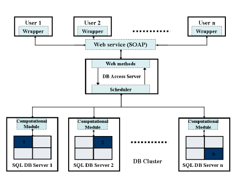
Figure 1: The architecture of the turbulence database cluster.

From the point of view of a user, it is desirable that a database cluster should, among others: (1) be available to the public by allowing remote access through the network; (2) provide flexible and comprehensive data processing functionalities inside the database so as to reduce data download; (3) be compatible with different platforms; (4) be compatible with the programs and tools that have been developed and used by the researchers in the past; (5) be efficient. With these requirements in mind, a cluster of database servers has been designed according to the diagram shown in Fig. 1. A time series of $1024^{3}$ DNS data of isotropic, steady state turbulence is stored in the database cluster. A total of 1024 time steps, or $27$ terabytes of data, have been loaded. The data are partitioned spatially and placed on different database nodes in the cluster. Most of the nodes have two dual core AMD Opteron processors with 4GB memory, while some have two Intel Xeon quad-core processors. The operating system is 64-bit Microsoft Windows 2003 Server. The dataset is managed by Microsoft SQL Sever 2005 (64 bit). For more details see [9].

The users connect to the database via the Internet (at http://turbulence.pha.jhu.edu) and access the data through a data access server. The communication between the users and the data access server adopts the Web service model. The data access server is also the head-node of the database cluster. It communicates with other database servers (nodes) in the cluster over high-speed local area network. The data access server is a mediator: it receives requests from the users, breaks the request into parts and sends the parts to the individual database nodes. The majority of the calculations are done in the Computational Module in each node, embodying the “move the program to the data” principle in scientific database design [5]. High efficiency is achieved through a high degree of parallelism. The details of the turbulence dataset and details of several components of the database cluster are described in the following several sub-sections.

2.1 Turbulence data set

The data is from a DNS of forced isotropic turbulence on a $1024^{3}$ periodic grid in a $[0,2\pi]^{3}$-domain, using a pseudo-spectral parallel code. Time integration of the viscous term is done analytically using the exact integrating factor. The other terms are integrated using a second-order Adams-Bashforth scheme and the nonlinear term is written in vorticity form [26]. The simulation is de-aliased using phase-shift and $2\sqrt{2}/3$ spherical truncation [27], so that the effective maximum wavenumber is about $k_{\rm max}=1024\sqrt{2}/3\approx 482$. Energy is injected by keeping constant the total energy in modes such that their wave-number magnitude is less or equal to 2. The simulation time-step is $\Delta t=0.0002$. After the simulation has reached a statistical stationary state, $1024$ frames of data, which includes the 3 components of the velocity vector and the pressure, are generated in physical space and ingested into the database. The data are stored at every 10 DNS time-setps, i.e. the samples are stored at time-step $\delta t=0.002$. The duration of the stored data is $1024\times 0.002=2.048$, i.e. about one large-eddy turnover time since $T=L/u^{\prime}\approx 2.02$ ($L$ is the integral scale). The parameters of the simulation are given in Table 1. The total kinetic energy, dissipation rate, and energy spectra are computed by averaging in time between $t=0$ and $t=2.048$.

Resolution, $N$		1024
Viscosity, $\nu$		0.000185
Time step of DNS, $\Delta t$		0.0002
Time interval between stored data sets, $\delta t$		0.002
Total kinetic energy, $E_{\rm tot}=\langle\sum\limits_{\bf k}\frac{1}{2}\hat{\bf u}\cdot\hat{\bf u}^{*}\rangle_{\rm t}$		0.695
Mean dissipation rate, $\epsilon=\langle\sum\limits_{\bf k}\nu k^{2}\hat{\bf u}\cdot\hat{\bf u}^{*}\rangle_{\rm t}$		0.0928
r.m.s. velocity fluctuation, $u^{\prime}=\sqrt{\frac{2}{3}E_{\rm tot}}$		0.681
Taylor micro length scale, $\lambda=\sqrt{15\nu u^{\prime 2}/\epsilon}$		0.118
Taylor micro-scale Reynolds number, $Re_{\lambda}=u^{\prime}\lambda/\nu$		433
Kolmogorov length scale, $\eta_{K}=(\nu 3/\epsilon)^{1/4}$		0.00287
Kolmogorov time scale, $\tau_{K}=(\nu/\epsilon)^{1/2}$		0.0446
Integral length scale, $L=\frac{\pi}{2u^{\prime 2}}\int\frac{E(k)}{k}dk$		1.376
Integral time scale, $T=\frac{L}{u^{\prime}}$		2.02

Table 1: The parameters of the DNS data in the turbulence database.

Figure 2 shows the radial energy spectrum computed from the simulation and averaged between $t=0$ and $t=2.048$. Figures 3 and 4 show time-series of the total turbulent kinetic energy and Taylor-scale based Reynolds numbers starting near the simulation initial condition. The values corresponding to the data in the database are for $t>0$ and are shown in solid line portions.

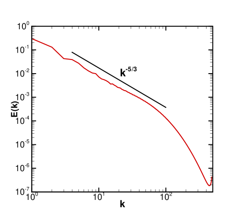
Figure 2: Radial kinetic energy spectrum, averaged in time between $t=0$ and $2.048$.

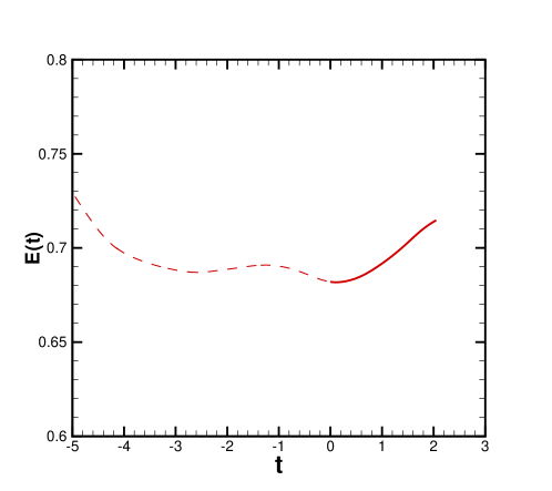
Figure 3: Total kinetic energy as function of time. Dashed line is times before ingestion into database. Data corresponding to the database is show using solid line between $t=0$ and $2.048$.

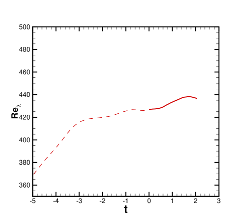
Figure 4: Taylor micro-scale Reynolds number as function of time. Dashed line is times before ingestion into database. Data corresponding to the database is show using solid line between $t=0$ and $2.048$.

2.2 User interface

The Web service model is adopted to implement the communication between the users and the database. The Web service technique makes possible the automatic interaction between the database and a computational program running on a user’s desktop or laptop computer. The program can fetch data from the database whenever data are needed, while performing further data analysis on the local machine between data requests. To realize this functionality, the user interface includes two parts: the Web-service methods implemented on the database access server and the client-side wrapper interface. Web-service methods are based on the standard protocol SOAP (Simple Object Access Protocol) [28]. They can be easily called from some modern programming languages such as Java or C#. Unfortunately, other languages need additional libraries to use Web-services. For example while recent versions of MATLAB offer integrated Web-service support, it is still necessary to provide a wrapper function to perform complex data type conversions. For FORTRAN and C codes running in UNIX, Linux or MacOS, we have developed and provided FORTRAN and C wrapper interfaces to the gSOAP library [29], which establishes the communication between the client code and the Web-service methods.

A list of Web-service methods are implemented on the data access server [30]. These methods provide the entry points to the processing functions implemented on the database servers (the “Computational module” in Fig. 1, will be explained below). The data access server has the knowledge of the data partition among the database servers. When a request is received from the user, the data access server find out on which database servers the requested data is stored, and then break the request into parts and send each part to the corresponding server. Upon receiving the requests, the Computational Modules on the database servers are invoked to perform necessary computations and return the requested data to the Web-service methods on the data access server (see Fig. 1). The Web-service methods then communicate the data back to user programs.

2.3 Processing function set

A set of processing functions are implemented as stored procedures on the database servers, referred to as Computational Module in Fig. 1. Microsoft SQL Server’s Common Language Runtime (CLR) [31] integration allows these stored procedures programmed in C#. They are intended to provide for the users a comprehensive and yet compact set of tools to process the data in the database. In turbulence research, the questions being asked and techniques used in data analysis are highly specific to the client and often vary from one client to another. Therefore, the design of these functions is not straightforward. One has to consider the trade-off between generality and efficiency. From our experience, we consider the most basic common tasks in data analysis are to calculate some basic flow parameters on a set of spatial locations. The basic functions supported thus include evaluating the velocity $u_{i}$ and pressure $p$ on arbitrary spatial locations, and also their spatial differentiation for first and second derivatives, as well as spatial and temporal interpolation. Specifically, the functions allow evaluating the full velocity gradient tensor $A_{ij}=\partial u_{i}/\partial x_{j}$ as well as the pressure gradient $\partial p/\partial x_{i}$. For second derivatives, the pressure Hessian $\partial^{2}p/\partial x_{i}\partial x_{j}$, Laplacian of velocity $\nabla^{2}u_{i}$, and full velocity Hessian, $\partial^{2}u_{i}/\partial x_{p}\partial x_{q}$, are supported. Due to the need for spatially localized differentiation stencils, derivatives are evaluated using centered finite differencing of 4th, 6th and 8th orders. Spatial interpolation is performed using Lagrange polynomial interpolation of various orders (also 4th, 6th and 8th order). Temporal interpolation is done using Cubic Hermite Interpolation. Details of these functions are provided in Appendix B, C, and D.

2.4 Data indexing, partition, and workload schedule

Indexing the spatial data consists of mapping the three dimensional spatial data onto a one dimensional array. Maintaining good locality of the spatial data is one of the favorable attributes of the mapping. That is, if two points are close to each other in the 3D space, their positions in the one dimensional array should also be close. This is clearly an advantage for applications accessing coherent regions in the physical space, such as structure identification and filtering. In our system, the data is indexed according to the Z-order (also known as Morton-order)[32], for it maintains fairly good locality and is simple to implement and calculate. The Z-index of each grid point in the computational mesh is calculated from the three-dimensional index of the point using bit-interleaving [9]. The concepts of Z-order and Z-index are illustrated in Fig. 5 with a two-dimensional grid. For our $1024^{3}$ DNS data, we need $30$ bits to index all the points. The Z-index of each point has $30$ bits in its binary representation.

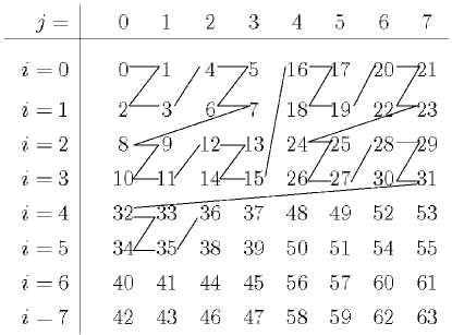
Figure 5: Table of Z-indices of a two-dimensional $8\times 8$ grid. $i$ and $j$ are the indices of the grid points along $x$ and $y$ directions, respectively. The values in the table are the Z-indices of the grid points calculated using bit-interleaving. The Z-order curve connects the grid points according to Z-order, i.e., in the order of increasing Z-indices. The same order is used to index the data in the database.

The spatial partition and organization of the data is also based on the Z-order of the data. To optimize I/O operations, we divide the whole data set into “atoms” of a fixed size (see below). The atom is the fundamental unit of I/O operations, i.e., whenever some data is needed, a whole atom is read into the memory. The atoms are stored on disk and indexed using a standard database B+-tree index. The B+-tree index of an atom is given by the six common middle bits of the binary representations of the Z-indices of the data points within the atom (see [9] for details). Using these bits as the search key in the B+-tree ensures that the atoms that are contiguous in the Z-order are also contiguous in the index. Given the good locality of the Z-order, this data structure thus supports fast access to contiguous region in the physical space. Similarly, the allocation of the atoms on different data servers is also determined by the Z-indices of the data points.

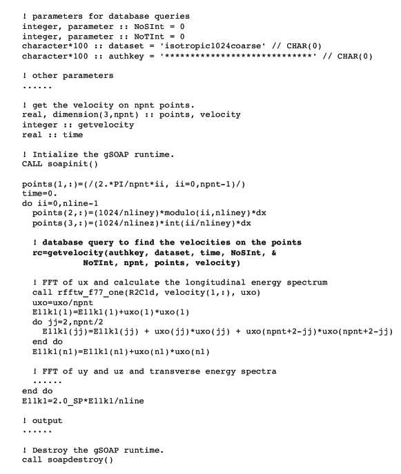
Figure 6: Snippet of the FORTRAN code running on local user machine. Bold font highlights the lines invoking the Web-service method. The authkey has been intentionally marked out.

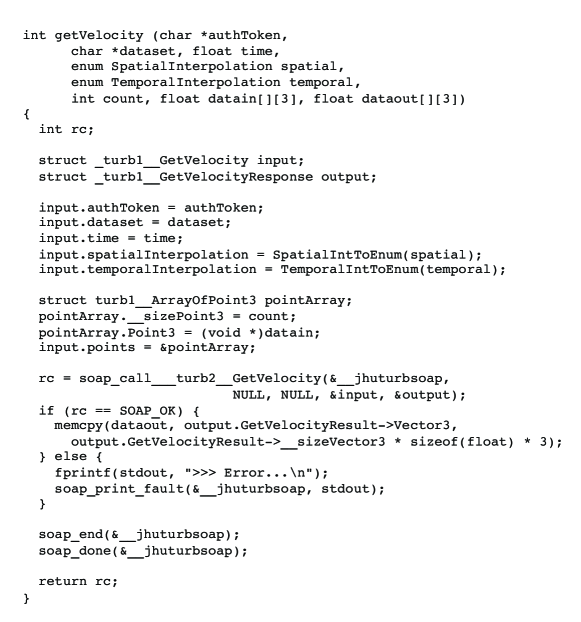
Figure 7: The C wrapper interface for the FORTRAN code. It invokes the gSOAP libraries to invoke the Web-service method.

The size of the atoms is chosen based on two considerations. We have found that using an atom of size $64^{3}$ data points as the fundamental I/O unit is the most efficient because it balances the memory and disk performance [9] in our application. However, as we mentioned before, a frequent operation required by the processing functions is interpolation. For 8th order interpolation, a blob of $8^{3}$ data points need to be accessed to obtain the interpolated value at one point. Given the high frequency of this operation, it is highly desirable to avoid data transfer between different data servers during this operation, which would incur significant overhead. This is done by “edge replication” on the atoms. Specically, we divide the data space into $(1024/64)^{3}=16^{3}$ cubes of size $64^{3}$. An atom contains a cube in its center, and an edge of length 4 on each side of the cube. Each atom thus has $72^{3}$ data points, with edges replicated from the neighoring atoms. This way, it is guaranteed that each interpolation operation can be finished with no more than one atom being read [9].

The Z-order indexing scheme is also used to schedule workload. As introduced above, the generic job request would be finding the values of some parameter on an array of spatial locations. To calculate the parameters at a point, the data in a small region around the point are accessed and need to be read from the hard drive. To minimize the amount of data reading, the spatial locations, and thus the data queries, are grouped according to the Z-order. Combined with data caching, where an atom of data is kept in the memory until another atom has to be loaded, this scheduling guarantees the same data atom is loaded into memory only once per job request.

3 Preliminary numerical tests

While loading the data onto the database cluster a number of point-by-point checks are made. In order to illustrate the usage of the database system, and also as a further check against, for example, the potential errors occurred during loading the data into the database, three basic groups of quantities are calculated using the database. The first group is the longitudinal and transverse one-dimensional (1D) energy spectra. The longitudinal spectrum is defined as $E_{11}(k_{1})=\langle\hat{u}_{1}(k_{1}^{*})\hat{u}_{1}(k_{1})\rangle$, where $\hat{u}_{1}(k_{1})$ is the one-dimensional Fourier transformation of the $x$ component of the velocity along the $x$ direction. The average is taken over the $(y,z)$ plane. Similarly, the two transverse spectra are defined as $E_{22}(k_{1})=\langle\hat{u}_{2}(k_{1}^{*})\hat{u}_{2}(k_{1})\rangle$ and $E_{33}(k_{1})=\langle\hat{u}_{3}(k_{1}^{*})\hat{u}_{3}(k_{1})\rangle$, where $\hat{u}_{2}$ and $\hat{u}_{3}$ are one-dimensional Fourier transformations of the $y$ and $z$ components of the velocity, respectively. The second group of tests is the PDFs of the longitudinal and transverse velocity gradients. The longitudinal velocity gradients are the components of $A_{ij}$ when $i=j$, while the others are considered transverse ones. The third one is the joint PDF of the two tensor invariants of the velocity gradient $R\equiv-A_{ij}A_{jk}A_{ki}/3$ and $Q=-A_{ij}A_{ji}/2$[25]. The tear-drop shape of the joint PDF of these quantities is a well-known feature of turbulence [25, 21, 24, 23]. These three basic groups are evaluated in two separate ways and compared: The first is in the traditional way, which we will call “in-core” analysis. The in-core analysis is done on the cluster where the data are generated, and the raw data are the Fourier components of the velocity fields before they are transformed and loaded into the database. The velocity gradients are calculated in the Fourier space using spectral derivatives. The second approach uses the data stored in the database and uses database queries. In particular, the velocity gradients are obtained using the $6$th order centered finite differencing option (see Appendix B). Interpolation of the velocity is done using 6th-order Lagrange polynomial option when necessary (see Appendix C). In order to remove possible differences resulting from statistical sampling, data on exactly the same spatial locations are used in both methods.

The 1D spectra are calculated based on the velocity along particular lines across the domain. These are obtained by invoking the Web-service method GetVelocity. We take $512$ grid lines along the $x$ direction at $32\times 16$ $(y,z)$ locations. The $32\times 16$ locations are distributed uniformly on the grids along both $y$ and $z$ directions, i.e., $32$ locations along $y$ direction and $16$ locations along $z$ direction. In each database query, the velocity vectors on the $1024$ grid points on one of the lines are fetched from the database. Therefore there are $512$ database queries in total, each fetching $1024$ points. For the analysis in this paper, only data at a single time, at $t=0$, is used. The one-dimensional FFT of the velocity data along each line is performed in the program running on the local user machine. The energy spectra are obtained by averaging over all the lines. The FORTRAN code snippet in Fig. 6, taken from the program running on the local user machine, shows how the database is typically used in an application. As is highlighted in the figure with bold font, the Web-service method is invoked from the computational program through a wrapper function having the same name GetVelocity, as if it is another function implemented on the same computer. The wrapper function takes the time, the number of points, the order of Lagrange interpolation to be used, and the $x$, $y$, and $z$ coordinates of the points as input parameters. The three velocity components on the requested points are returned. The C wrapper function, shown in Fig. 7, invokes the gSOAP library to invoke the Web-service method implemented on the data access server.

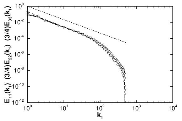
Figure 8: One-dimensional energy spectra calculated through database queries (lines) and calculated in-core (symbols). Solid line and squares: $E_{11}(k_{1})$, dashed and diamonds: $(3/4)E_{22}(k_{1})$, dash-dotted and gradients: $(3/4)E_{33}(k_{1})$. Thin dashed line has slope $-5/3$.

Notice that the data points we are using are all on the grids. Because there is no interpolation error for the values of the velocity on these points, this calculation could be compared with the in-core calculation and serves as a low-level check for the correctness of the data loading process. The result is shown in Fig. 8. The results calculated from the database are equal to those calculated in-core, suggesting that there was no error in loading the data.

The spectra show a narrow inertial range, in which the longitudinal and the rescaled transverse spectra overlap. The rescaled transverse spectra fall slightly above the longitudinal one towards the viscous range. The two transverse spectra are identical to each other except that slight difference can be seen at the lowest wavenumber. These features are all consistent with other DNS and experimental results (see, e.g., [33]). As a result of dealiasing, the spectra extend only to a wavenumber around 482, as noted before.

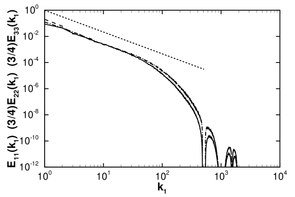
Figure 9: One-dimensional energy spectra calculated through database queries using $4096$ data points on each line with spatial interpolation. Line patterns same as in Fig. 8.

To illustrate the effects of Lagrange polynomial interpolation, another case with 512 lines and $4096$ points on each line is also calculated. The lines are chosen to be the same as in the previous case. The 4096 points are uniformly distributed on each line, and one in every four points falls on the grids. The $6$th order Lagrange interpolation scheme is used. As is shown in Fig. 9, the range of the spectra extends beyond the maximal resolved wavenumber in the simulation (about 482) to a value of around 2000. The oscillating lobes observed between wavenumbers 482 and 2000 are the spectral signature of the Lagrange interpolant polynomials. As a consequence of the smoothness of the interpolants, very little energy is contained in high wavenumber lobes, as one can see by comparing Fig. 8 and 9.

The PDFs of the velocity gradients and the joint PDF of $R$ and $Q$ are calculated in a similar way, except that the Web-service method invoked is GetVelocityGradient, instead of GetVelocity. The database queries return values for each element of the velocity gradient tensor, at every point requested. The velocity gradient tensor elements are calculated inside the database. In this case data on $256^{3}$, or about 17 million, spatial locations are requested. The points are again on the grids, and are equally spaced along each direction.

The results are plotted in Figs. 10 and 11. Also plotted are the results calculated in-core, in which the velocity derivatives are calculated from the Fourier components of the velocity field, and then transformed into physical space. The figure shows that there is very good agreement between the results. The minor differences are due to slight differences in the 6th-order finite difference and the spectral evaluations of the gradients. The results are also in good agreement with the results reported in the literature (see, for example, [34] and [24]).

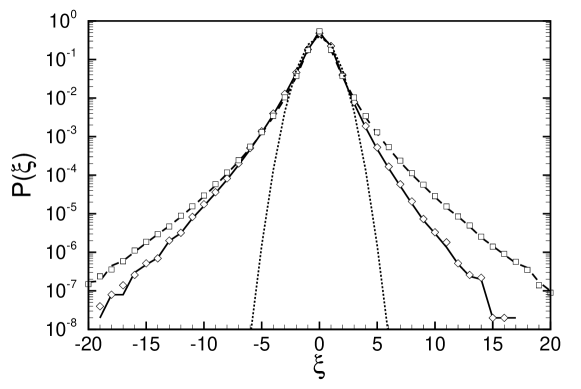
Figure 10: PDF of longitudinal (solid line and diamonds) and transverse (dashed line and squares) velocity gradients, normalized by rms values. Lines are calculated from database queries and symbols are from in-core calculations. The dotted line is Gaussian distribution.

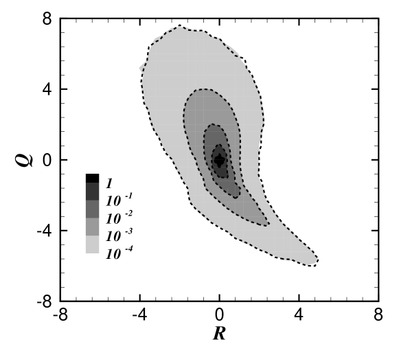
Figure 11: The contour plot of the joint PDF of $R$ and $Q$. Dashed lines: in-core calculations. Grey-scaled contours: database queries, in which $R$ and $Q$ are calculated on the local machine with the velocity gradient data fetched from the database.

The time taken to calculate the energy spectra is about 16 minutes for $512\times 1024$ points, and 26 minutes for $512\times 4096$ points. These numbers are quite encouraging for an initial implementation that has much room for additional optimizations.

To provide a more complete characterization of the presently achievable access speeds as function of the size of the request, additional experiments are carried out. Calls to the database are issued over the Internet from a FORTRAN program running on a desktop computer at JHU. Access times are measured as function of the number of points, $N_{p}$, at which data are requested. Three spatial arrangements of the points are considered: (a) $N_{p}$ points arranged on a cubic lattice, with $\sim N_{p}^{1/3}$ points on each side; (b) all $N_{p}$ points along a single line, with points separated by $2\pi/N_{p}$; and (c) $N_{p}$ positions at random positions over the entire domain (uniform probability density for each coordinate between $0$ and $2\pi$). Figures 12, 13 and 14 show the resulting access times in seconds, as function of $N_{p}$ for the three cases, respectively. For each spatial arrangement of the points, four types of data are requested. (1) three components of velocity (using GetVelocity), without spatial nor temporal interpolation; (2) nine velocity gradient tensor elements (using GetVelocityGradient), evaluated using 8th-order centered finite differencing but without spatial nor temporal interpolation; (3) pressure Hessian (using GetPressureHessian), evaluated using 4th-order centered finite differencing and 4th-order Lagrange Polynomial interpolation in space, by without temporal interpolation; and finally (4) velocity vector and pressure (using GetVelocityAndPressure), with 6th-order Lagrange Polynomial interpolation in space and Piecewise Cubic Hermite Interpolation Polynomial method for time. The corresponding access times as function of $N_{p}$ are indicated with different symbols in Figs. 12-14.

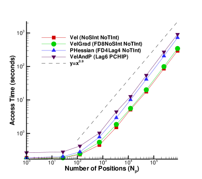
Figure 12: Access times (in seconds) measured as function of request size (number of points $N_{p}$), when the $N_{p}$ points are arranged on a cubic lattice of size $\sim N_{p}^{1/3}$. Different symbols denote different request types, including GetVelocity, GetVelocityGradient, GetPressureHessian, and GetVelocityAndPressure. Different combinations of order of interpolation and differentiation are also tested as indicated in the figure.

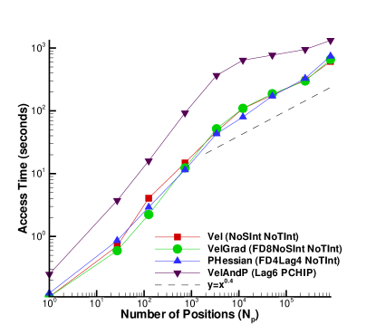
Figure 13: Access times (in seconds) measured as function of request size (number of points $N_{p}$), when the $N_{p}$ points are arranged along a single line with a separation between points of $2\pi/N_{p}$. Different symbols are the same as in Fig. 12.

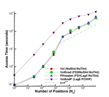
Figure 14: Access times (in seconds) measured as function of request size (number of points $N_{p}$), when the $N_{p}$ points are distributed randomly in the entire dataset. Different symbols are the same as in Fig. 12.

In case (a), not surprisingly, the function evaluation using both spatial and temporal interpolation is the most time-consuming while the one without any interpolation is fastest. In this case, when the number of points requested increases, the access time increases as $\sim N_{p}^{0.9}$, i.e. almost linearly. In cases (b) and (c), there is not as much difference as in case (a) among the function evaluations without temporal interpolation, but the one with temporal interpolation still takes more access time. In the latter two cases, the access time increases as $\sim N_{p}^{0.4}$ for $N_{p}$ above $\sim 3000$. Comparing the three cases, we can observe that when points are arranged as cubes, it takes the least access time for moderate size requests. The reason is that much of the data then typically falls within only a few of the stored atoms, decreasing the amount of data that needs to be read from disks. As can be seen, access times depend upon the details of the data arrangement, interpolation type and the size of the request. Of course, it also depends on the client’s network speed, etc.

4 Analysis of the advected delta-vee system

In this section, the database is used to analyze the advected delta-vee system derived in Ref. [10]. For the convenience of the readers, the derivation of the system is briefly reviewed first. We restrict ourselves to dynamics in three dimensional space.

The advected delta-vee system decribes the Lagrangian evolution of the longitudinal and transverse velocity increments (or more precisely, the longitudinal and transverse velocity gradient multiplied by a small and fixed displacement). Specifically, for an incompressible velocity field $\overline{u}_{i}({\bf x},t)$ filtered at scale $\Delta$ and velocity gradient $\overline{A}_{ij}\equiv\partial\overline{u}_{i}/\partial x_{j}$, consider a displacement vector ${\bf{r}}(t)$, and the unit vector in its direction $\hat{\bf r}={\bf r}/r$. The longitudinal and the magnitude of the transverse components of the ‘velocity increment’ vector along this direction across a fixed distance $\ell<\Delta$ are defined as

$$\delta u\equiv\ell~{}\overline{A}_{rr}\equiv\ell~{}\overline{A}_{ik}~{}\hat{r}_{k}~{}\hat{r}_{i},\quad\delta v\equiv\ell\left|P_{ij}({\bf r})~{}\overline{A}_{jk}~{}\hat{r}_{k}\right|,$$ (1)

where $\overline{A}_{rr}\equiv\overline{A}_{ik}\hat{r}_{k}\hat{r}_{i}$ is the velocity gradient along the direction $\hat{\bf r}$, and $P_{ij}({\bf r})\equiv\delta_{ij}-\hat{r}_{i}\hat{r}_{j}$ is the projection operator. For a detailed sketch illustrating these definitions, see Fig. 1 of Ref. [10].

Using the equations for the line element $r_{i}$ and the filtered velocity gradient $\overline{A}_{ij}$, one can derive from the definitions of $\delta u$ and $\delta v$ the following equations (for details see [10, 11]):

$$\frac{d\delta u}{dt} = -{\frac{1}{3}\delta u^{2}}~{}{\ell}^{-1}+{\delta v^{2}}~{}{\ell}^{-1}+Q^{-}\ell+Y,$$ (2)

$$\frac{d\delta v}{dt} = -{2~{}\delta u~{}\delta v}~{}{\ell}^{-1}+Z,$$ (3)

where $d/dt$ indicates material derivative. Also, $Y=\ell H_{ij}\hat{r}_{i}\hat{r}_{j}$ and $Z=\ell H_{ij}\hat{r}_{j}\hat{e}_{i}$, in which ${\bf\hat{e}}$ is a unit vector in the direction of the transverse velocity-increment component (perpendicular to $\hat{\bf r}$) and $H_{ij}=-(\partial^{2}_{ij}\overline{p}-\frac{1}{3}\delta_{ij}\partial^{2}_{kk}\overline{p})-(\partial^{2}_{jk}\tau_{ik}-\frac{1}{3}\delta_{ij}\partial^{2}_{lk}\tau_{lk})+\nu\partial^{2}_{kk}\overline{A}_{ij}+(\partial_{j}\overline{f}_{i}-\frac{1}{3}\delta_{ij}\partial_{k}\overline{f}_{k})$. $H_{ij}$ is the anisotropic part of the gradients of pressure, sub-grid scale, viscous, and external forces, with $\tau_{ij}\equiv\overline{u_{i}u}_{j}-\overline{u}_{i}\overline{u}_{j}$ being the sub-grid scale (SGS) stress. $Q^{-}$ is defined as $Q^{-}=-\overline{A}_{ij}\overline{A}_{ji}/3-2\delta u^{2}/3\ell^{2}$ (see [11] for details).

Eqs. 2 and 3 are called the “advected delta-vee system”. In the system, the nonlinear self-interaction terms are closed, while $Q^{-}$, $Y$ and $Z$ are not. As shown in [11], the truncated system retaining only the nonlinear self-interaction terms is already able to predict a number of well-known, important intermittency trends. Nevertheless, the unclosed terms have to be included through physically realistic models in order for the system to predict quantitative features of intermittency and to reach stationary statistical states. As the first step in constructing such models, here we will now analyze the unclosed terms using the DNS data in the database. Since filtering operations are not yet supported by the database, the analysis is restricted to unfiltered DNS data and the results pertain to velocity increments across distances on the order of the Kolmogorov scale. Therefore the term corresponding to SGS force in $H_{ij}$ will be absent, and the filtered quantities will recover their unfiltered values. Hence we will drop in the following the overbar in the symbols. For example, $\overline{A}_{ij}$ will be replaced by $A_{ij}$ and so on.

The analysis is based on the evolution equation for the joint PDF of $\delta u$ and $\delta v$, which has been derived in appendix A:

$$\frac{\partial P}{\partial t}+\frac{\partial}{\partial\delta u}\left[(\delta v^{2}-\frac{1}{3}\delta u^{2})P\right]+\frac{\partial}{\partial\delta v}\left[-2\delta u\delta vP\right]+\frac{\partial}{\partial\delta u}\left[\left\langle\left.Q^{-}\right|\delta u,\delta v\right\rangle P\right]$$ (4)

$$+ \frac{\partial}{\partial\delta u}\left[\left\langle\left.Y\right|\delta u,\delta v\right\rangle P\right]+\frac{\partial}{\partial\delta v}\left[\left\langle\left.Z\right|\delta u,\delta v\right\rangle P\right]+3(\delta u-\langle\delta u\rangle)P=0.$$

In Eq. 4, $P\equiv P(\delta u,\delta v;t)$ is the joint PDF of $\delta u$ and $\delta v$ at time $t$. The equation describes the balance produced by three different types of terms: the unsteady term $\partial P/\partial t$, the measure correction term ${\rm S}\equiv 3(\delta u-\langle\delta u\rangle)P$, and the probability flux terms. For stationary turbulence, the unsteady term is zero. To simplify later analysis, we then write ${\mbox{\boldmath$\nabla$}}\cdot{\bf W}+S=0$, with ${\bf W}={\bf W}_{\rm sc}+{\bf W}_{\rm Q}+{\bf W}_{\rm p}+{\bf W}_{\rm v}+{\bf W}_{\rm f}$. The following symbols denote the probability fluxes caused by different physical mechanisms:

$$\begin{array}[]{ll}{\bf W}_{\rm sc}=[\delta v^{2}-\delta u^{2}/3,-2\delta u\delta v]P,&{\bf W}_{\rm Q}=[\left\langle\left.Q^{-}\right|\delta u,\delta v\right\rangle,0]P,\\ {\bf W}_{\rm p}=[\left\langle\left.Y_{p}\right|\delta u,\delta v\right\rangle,\left\langle\left.Z_{p}\right|\delta u,\delta v\right\rangle]P,&{\bf W}_{\rm v}=[\left\langle\left.Y_{v}\right|\delta u,\delta v\right\rangle,\left\langle\left.Z_{v}\right|\delta u,\delta v\right\rangle]P,\\ {\bf W}_{\rm f}=[\left\langle\left.Y_{f}\right|\delta u,\delta v\right\rangle,\left\langle\left.Z_{f}\right|\delta u,\delta v\right\rangle]P,&\\ \end{array}$$ (5)

in which $Y$ and $Z$ have each been separated into three parts:

$$\begin{array}[]{ll}\displaystyle{Y_{p}=-\hat{r}_{i}\hat{r}_{j}\partial^{2}_{ij}p+(1/3)\partial^{2}_{kk}p},&Z_{p}=-\hat{e}_{i}\hat{r}_{j}\partial^{2}_{ij}p,\\ \displaystyle{Y_{v}=\nu\hat{r}_{i}\hat{r}_{j}\partial^{2}_{kk}A_{ij}},&Z_{v}=\nu\hat{e}_{i}\hat{r}_{j}\partial^{2}_{kk}A_{ij},\\ \displaystyle{Y_{f}=\hat{r}_{i}\hat{r}_{j}\partial_{j}f_{i}-(1/3)\partial_{k}f_{k}},&Z_{f}=\hat{e}_{i}\hat{r}_{j}\partial_{j}f_{i}.\end{array}$$ (6)

These terms represent, respectively, the effects of pressure, viscous diffusion, and external force. Note that in the $Z$’s the contributions from the isotropic parts of the tensors are zero because $\hat{\bf r}$ is orthogonal to $\hat{\bf e}$. The same is true in $Y_{v}$ due to incompressibility.

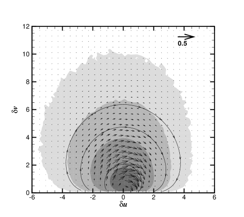
Figure 15: The vector plot of ${\bf W}_{\rm sc}$, the probability flux generated by the self-interaction terms. Several stream traces are plotted. The contour plot is $P(\delta u,\delta v)$, the joint PDF of $\delta u$ and $\delta v$.

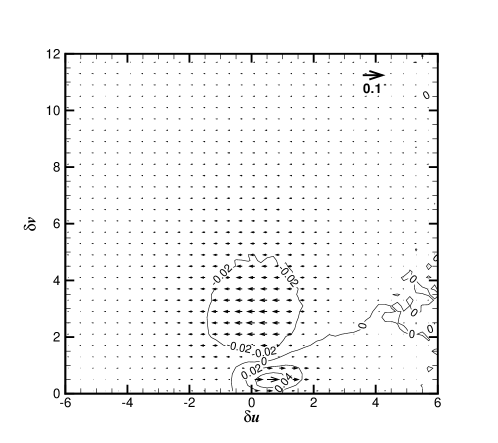
Figure 16: The vector plot of ${\bf W}_{\rm Q}$, the probability flux generated by the $Q^{-}$ term. By definition, all the vectors are parallel to $\delta u$ axis. Several contours of the magnitude of the vectors are plotted.

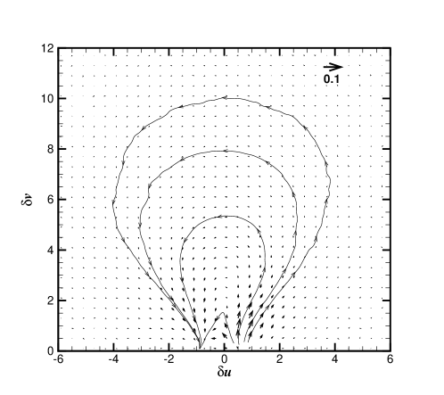
Figure 17: The vector plot of ${\bf W}_{\rm p}$, the probability flux generated by the anisotropic part of the pressure Hessian.

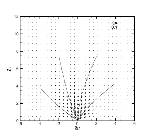
Figure 18: The vector plot of ${\bf W}_{\rm v}$, the probability flux generated by the viscous diffusion term.

The joint pdf $P(\delta u,\delta v)$ and the flux terms in the above joint PDF equation are calculated using the turbulence database described in previous sections, except for the flux produced by the forcing term, which is not included in the analysis. The forcing term can not, at this stage, be obtained directly from the database. But since the forcing only occurs at large scales its direct effect on the terms related to the small-scale dynamics of velocity gradient are negligible, and its omission does not alter the conclusions to be drawn. Also, when calculating the viscous diffusion term ${\bf W}_{\rm v}$, $\nabla^{2}A_{ij}$ is needed, which entails third order differentiation of the velocity field. This is a rather specific operation and, for now, was not considered generic enough to be included in the processing function set of the database. Therefore, in this analysis $\nabla^{2}A_{ij}$ is calculated on the local client-side computer using the data of $A_{ij}$ obtained from database queries at various grid points, and then evaluating the $4$th order central finite difference approximation to the Laplacian $\nabla^{2}$. The $(\delta u,\delta v$) phase-space is binned into $80\times 80$ boxes and conditional averages are computed by averaging over about half of a million randomly chosen datapoints, and $50$ random directions of $\hat{\bf r}$ at $t=0$.

The probability flux generated by the closed self-interaction terms is plotted in Fig. 15. The contour plot layered under the vector plot is the joint PDF of $\delta u$ and $\delta v$. The joint PDF displays the correct skewness towards negative $\delta u$ direction. By construction, the stream traces in Fig. 15 have the same shapes as the phase orbits of the truncated system (with $Q^{-}$, $Y$, and $Z$ neglected), as plotted in Fig. 5(b) in [11]. As explained in [10, 11], due to the negative quadratic term $-\delta u^{2}/3$ in Eq. 2, negative values of $\delta u$ are continuously amplified, while positive fluctuations tend to be decreased. This mechanism, referred to as the self-amplification of the longitudinal velocity increments, is thus responsible for generating the negative skewness in $\delta u$. On the other hand, the right-hand side of Eq. 3 becomes positive when $\delta u$ is negative. Therefore, a large negative value of $\delta u$ will produce exponential growth in $\delta v$, thus leading to strong fluctuation in $\delta v$. This mechanism for the generation of intermittency in the transverse velocity increment is called the cross amplification mechanism. The stream traces in Fig. 15 give an instructive illustration of the coupling between the two mechanisms. This figure, however, also shows that the self-interaction terms alone can not maintain a stationary distribution in $P(\delta u,\delta v)$. We expect that the other terms will tend to oppose the excessive growth of the intermittency produced by these two terms and enable the system to reach a stationary distribution.

Plotted in Fig. 16 through Fig. 18 are the probability fluxes generated by the $Q^{-}$ term, the anisotropic pressure Hessian term, and the viscous diffusion term, respectively. By definition, the $\delta v$ component of the flux ${\bf W}_{\rm Q}$ is zero, therefore all the vectors in Fig. 16 are parallel to the $\delta u$ axis. The lines in the figure are contours of the distribution of the non-zero (horizontal) component of the probability flux vector. Separated by the zero contour, the vectors in the lower right corner point to positive $\delta u$, while those above point to the negative direction. This combination shows a general tendency for the $Q^{-}$ term to oppose the effect of the self-interactions terms. Note however, in the negative $\delta u$ half plane, the vectors pointing to the negative $\delta u$ direction would strengthen the negative amplification of $\delta u$, and thus increase the intermittency in $\delta v$ due to the cross-amplification mechanism explained before. On the other hand, the stream traces of the flux generated by the pressure Hessian, shown in Fig. 17, have a similar shape as those in Fig. 15, but with opposite direction. It indicates that the main effect of the pressure Hessian is to reduce the intermittency generated by the self-interaction terms. Besides, we note that the stream traces show an interesting sink-source structure. Fig. 18 shows that the contribution of viscous diffusion is mainly to introduce a nearly linear damping effect, i.e., all vectors pointing to the origin.

5 Conclusions

In this paper, a new turbulence database system has been described. By applying database technologies, the system enables remote access to a DNS data set with 27 Terabytes, encapsulating a complete $1024^{4}$ space-time history of forced isotropic turbulence. The architecture of the system, including the user interface, processing function set, data indexing and partition, and work load scheduling, is explained. Test cases are presented to demonstrate the usage of the system, and to check against possible errors. The database thus provides a new platform for turbulence research, and a useful prototype for building large-scale scientific databases.

As an example for the application of the database, the advected delta-vee system introduced in [10, 11] is analyzed by accessing the database from a remote desktop computer. The analysis shows that the main effect of the unclosed terms in the system is to oppose the excessive growth of intermittency in the velocity increments produced by the nonlinear self-interaction terms. The various terms (isotropic pressure Hessian effect, deviatoric pressure Hessian term, and viscous term) show markedly different behaviors among themselves. While the detailed physics underlying these observations are not yet clear, the results imply that when closure models are constructed for these terms, they should be modeled separately. Specifically, the viscous term may be modeled using a simple relaxation towards the origin, but the pressure terms will require more elaborate closures.

Appendices

Appendix A Equation for the joint PDF of the longitudinal and transverse velocity increments

In this appendix, we will derive the equation for the joint PDF of $\delta u$ and $\delta v$, from the dynamic equations for $\delta u$ and $\delta v$ (Eqs. 2 and 3), and the equation for the length of the line element $r(t)$:

$$\frac{dr}{dt}=\delta u~{}r~{}\ell^{-1}.$$ (7)

Recall that the velocity increments are defined over a distance $\ell$ along the directions of evolving line elements $\bf r$. As noted in [10, 11], during their evolution the line elements tend to concentrate along the stretching directions of the flow field. Therefore, the joint PDF defined with equal weight on each trajectory in the $(\delta u,\delta v)$ phase space will put more weight on the velocity increments along the stretching directions. In order to obtain unbiased statistics, a measure correcting procedure has been proposed in [10]. Based on mass conservation, it was shown that when accumulating the statistics of $(\delta u,\delta v)$ at time $t$, each trajectory has to be weighed with a factor $[r_{0}/r(t)]^{3}$, where $r_{0}$ is the initial length of the line element. In terms of the joint PDF of $\delta u$ and $\delta v$, it implies that, assuming all the line elements initially having the same length $\ell$, the unbiased joint PDF of $\delta u$ and $\delta v$ can be formally written as

$$P(\delta u,\delta v;t)=\frac{1}{I(t)}\int_{0}^{+\infty}P_{3}(\delta u,\delta v,r;t)r^{-3}dr,$$ (8)

in which $P_{3}(\delta u,\delta v,r)$ is the traditional joint PDF of the three independent variables. $I(t)$ is a normalization factor, defined as:

$$I(t)\equiv\int_{-\infty}^{+\infty}\int_{0}^{+\infty}\int_{0}^{+\infty}P_{3}(\delta u,\delta v,r;t)r^{-3}d\delta u\,d\delta v\,dr.$$ (9)

From these definitions, the equation for $P$ can be derived from the Liouville equation for $P_{3}$

$$\frac{\partial P_{3}}{\partial t}+\frac{\partial}{\partial\delta u}(\left\langle\left.\delta\dot{u}\right|\delta u,\delta v,r\right\rangle P_{3})+\frac{\partial}{\partial\delta v}(\left\langle\left.\delta\dot{v}\right|\delta u,\delta v,r\right\rangle P_{3})+\frac{\partial}{\partial r}(\left\langle\left.\dot{r}\right|\delta u,\delta v,r\right\rangle P_{3})=0,$$ (10)

where $\dot{a}\equiv da/dt$ means material derivative. Multiplying Eq. 10 by $r^{-3}$ and integrating over $r$, one obtains

$$\frac{\partial I(t)P}{\partial t}\!\! + \!\!\frac{\partial}{\partial\delta u}\left[\int_{0}^{+\infty}\left\langle\left.\delta\dot{u}\right|\delta u,\delta v,r\right\rangle P_{3}r^{-3}dr\right]+\frac{\partial}{\partial\delta v}\left[\int_{0}^{+\infty}\left\langle\left.\delta\dot{v}\right|\delta u,\delta v,r\right\rangle P_{3}r^{-3}dr\right]$$ (11)

$$+ \!\!\int_{0}^{+\infty}r^{-3}\frac{\partial}{\partial r}(\left\langle\left.\dot{r}\right|\delta u,\delta v,r\right\rangle P_{3})dr=0.$$

By straightforward calculation, the first two integrals can be reduced to:

$$I(t)\left\langle\left.\delta\dot{u}\right|\delta u,\delta v\right\rangle P(\delta u,\delta v)$$ (12)

and

$$I(t)\left\langle\left.\delta\dot{v}\right|\delta u,\delta v\right\rangle P(\delta u,\delta v)$$ (13)

respectively. Using Eq. 7, the third one becomes

$$\int_{0}^{+\infty}r^{-3}\frac{\partial}{\partial r}(\delta urP_{3})dr=r^{-2}\delta uP_{3}|_{0}^{+\infty}-\int_{0}^{+\infty}\delta urP_{3}(-3)r^{-4}dr=3\delta uI(t)P,$$ (14)

assuming $\delta uP_{3}(\delta u,\delta v,r)$ approaches zero faster than $r^{2}$ for any $\delta u$, $\delta v$ when $r\to 0$. Thus, one obtains

$$\frac{\partial I(t)P}{\partial t}+I(t)\left[\frac{\partial}{\partial\delta u}(\left\langle\left.\delta\dot{u}\right|\delta u,\delta v\right\rangle P)+\frac{\partial}{\partial\delta v}(\left\langle\left.\delta\dot{v}\right|\delta u,\delta v\right\rangle P)+3\delta uP\right]=0.$$ (15)

Integrating the above equation over $\delta u$ and $\delta v$, the normalization condition for $P$ yields

$$\frac{dI(t)}{dt}+3I(t)\int_{-\infty}^{+\infty}\int_{0}^{+\infty}\delta uPd\delta ud\delta v=\frac{dI(t)}{dt}+3I(t)\langle\delta u\rangle=0,$$ (16)

if $\left\langle\left.\delta\dot{u}\right|\delta u,\delta v\right\rangle P$ and $\left\langle\left.\delta\dot{v}\right|\delta u,\delta v\right\rangle P$ tend to zero at the boundaries. Thus

$$\frac{\partial P}{\partial t} = \frac{1}{I(t)}\frac{\partial I(t)P}{\partial t}-\frac{P}{I(t)}\frac{dI(t)}{dt}$$ (17)

$$= -\left[\frac{\partial}{\partial\delta u}(\left\langle\left.\delta\dot{u}\right|\delta u,\delta v\right\rangle P)+\frac{\partial}{\partial\delta v}(\left\langle\left.\delta\dot{v}\right|\delta u,\delta v\right\rangle P)+3\delta uP\right]$$

$$+3\langle\delta u\rangle P.$$

Replacing $\delta\dot{u}$ and $\delta\dot{v}$ with Eq. 2 and 3 and rearranging the terms finally yields

$$\frac{\partial P}{\partial t}+\frac{\partial}{\partial\delta u}\left[\left(\delta v^{2}-\frac{1}{3}\delta u^{2}\right)P\right]+\frac{\partial}{\partial\delta v}\left[-2\delta u\delta vP\right]+\frac{\partial}{\partial\delta u}\left[\left\langle\left.Q^{-}\right|\delta u,\delta v\right\rangle P\right]$$ (18)

$$+ \frac{\partial}{\partial\delta u}\left[\left\langle\left.Y\right|\delta u,\delta v\right\rangle P\right]+\frac{\partial}{\partial\delta v}\left[\left\langle\left.Z\right|\delta u,\delta v\right\rangle P\right]+3(\delta u-\langle\delta u\rangle)P=0.$$

This is the equation for the joint PDF of $\delta u$ and $\delta v$. The last term on the LHS of the equation comes from the measure correction procedure. Note that we have assumed $\ell=1$.

Appendix B Documentation: database spatial differentiation

In this appendix, details are provided about the various options for spatial differentiations implemented in the database cluster. Below, $f$ denotes any one of the three components of velocity, $u$, $v$ or $w$, or pressure, $p$, depending on which function is called. $\Delta x$ and $\Delta y$ are the width of grid in $x$ and $y$ direction.

B.1 Options for GetVelocityGradient and GetPressureGradient

Figure 19: Illustration of data points along $x$ direction. The same approach is used in the $y$ and $z$ directions.

FD4: 4th-order centered finite differencing

With the edge replication of 4 data-points on each side, this option can be spatially interpolated using 4th-order Lagrange Polynomial interpolation.

$$\left.\frac{df}{dx}\right|_{x_{n}} = \frac{2}{3\Delta x}[f(x_{n+1})-f(x_{n-1})]-\frac{1}{12\Delta x}[f(x_{n+2})-f(x_{n-2})]$$ (19)

$$+O(\Delta x^{4})$$

FD6: 6th-order centered finite differencing

$$\left.\frac{df}{dx}\right|_{x_{n}} = \frac{3}{4\Delta x}[f(x_{n+1})-f(x_{n-1})]-\frac{3}{20\Delta x}[f(x_{n+2})-f(x_{n-2})]$$ (20)

$$+\frac{1}{60\Delta x}[f(x_{n+3})-f(x_{n-3})]+O(\Delta x^{6})$$

FD8: 8th-order centered finite differencing

With the edge replication of 4 data-points on each side, this is the highest-order finite difference option available.

$$\left.\frac{df}{dx}\right|_{x_{n}} = \frac{4}{5\Delta x}[f(x_{n+1})-f(x_{n-1})]-\frac{1}{5\Delta x}[f(x_{n+2})-f(x_{n-2})]$$ (21)

$$+\frac{4}{105\Delta x}[f(x_{n+3})-f(x_{n-3})]-\frac{1}{280\Delta x}[f(x_{n+4})-f(x_{n-4})]$$

$$+O(\Delta x^{8})$$

B.2 Options for GetVelocityLaplacian, GetVelocityHessian and GetPressureHessian

In this section, second derivatives finite difference evaluations are shown. The expressions are given for derivatives along single directions in terms of the $x$-direction, and mixed derivatives are illustrated on the $x$-$y$ plane. The same approach is used in the $y$ and $z$ directions, as well as in the $x$-$z$ and $y$-$z$ planes for the other mixed derivatives.

FD4: 4th-order centered finite differencing (can be spatially interpolated using 4th-order Lagrange Polynomial interpolation)

$$\left.\frac{d^{2}f}{dx^{2}}\right|_{(x_{m},y_{n})} = \frac{4}{3\Delta x^{2}}[f(x_{m+1},y_{n})+f(x_{m-1},y_{n})-2f(x_{m},y_{n})]$$ (22)

$$-\frac{1}{12\Delta x^{2}}[f(x_{m+2},y_{n})+f(x_{m-2},y_{n})-2f(x_{m},y_{n})]$$

$$+O(\Delta x^{4})$$

$$\left.\frac{d^{2}f}{dxdy}\right|_{(x_{m},y_{n})} = \frac{1}{3\Delta x\Delta y}[f(x_{m+1},y_{n+1})+f(x_{m-1},y_{n-1})$$ (23)

$$-f(x_{m+1},y_{n-1})-f(x_{m-1},y_{n+1})]$$

$$-\frac{1}{48\Delta x\Delta y}[f(x_{m+2},y_{n+2})+f(x_{m-2},y_{n-2})$$

$$-f(x_{m+2},y_{n-2})-f(x_{m-2},y_{n+2})]$$

$$+O(\Delta x^{4},\Delta y^{4})$$

FD6: 6th-order centered finite differencing

$$\left.\frac{d^{2}f}{dx^{2}}\right|_{(x_{m},y_{n})} = \frac{3}{2\Delta x^{2}}[f(x_{m+1},y_{n})+f(x_{m-1},y_{n})-2f(x_{m},y_{n})]$$ (24)

$$-\frac{3}{20\Delta x^{2}}[f(x_{m+2},y_{n})+f(x_{m-2},y_{n})-2f(x_{m},y_{n})]$$

$$+\frac{1}{90\Delta x^{2}}[f(x_{m+3},y_{n})+f(x_{m-3},y_{n})-2f(x_{m},y_{n})]$$

$$+O(\Delta x^{6})$$

$$\left.\frac{d^{2}f}{dxdy}\right|_{(x_{m},y_{n})} = \frac{3}{8\Delta x\Delta y}[f(x_{m+1},y_{n+1})+f(x_{m-1},y_{n-1})$$ (25)

$$-f(x_{m+1},y_{n-1})-f(x_{m-1},y_{n+1})]$$

$$-\frac{3}{80\Delta x\Delta y}[f(x_{m+2},y_{n+2})+f(x_{m-2},y_{n-2})$$

$$-f(x_{m+2},y_{n-2})-f(x_{m-2},y_{n+2})]$$

$$+\frac{1}{360\Delta x\Delta y}[f(x_{m+3},y_{n+3})+f(x_{m-3},y_{n-3})$$

$$-f(x_{m+3},y_{n-3})-f(x_{m-3},y_{n+3})]$$

$$+O(\Delta x^{6},\Delta y^{6})$$

FD8: 8th-order centered finite differencing

$$\left.\frac{d^{2}f}{dx^{2}}\right|_{(x_{m},y_{n})} = \frac{792}{591\Delta x^{2}}[f(x_{m+1},y_{n})+f(x_{m-1},y_{n})-2f(x_{m},y_{n})]$$ (26)

$$-\frac{207}{2955\Delta x^{2}}[f(x_{m+2},y_{n})+f(x_{m-2},y_{n})-2f(x_{m},y_{n})]$$

$$-\frac{104}{8865\Delta x^{2}}[f(x_{m+3},y_{n})+f(x_{m-3},y_{n})-2f(x_{m},y_{n})]$$

$$+\frac{9}{3152\Delta x^{2}}[f(x_{m+4},y_{n})+f(x_{m-4},y_{n})-2f(x_{m},y_{n})]$$

$$+O(\Delta x^{8})$$

$$\left.\frac{d^{2}f}{dxdy}\right|_{(x_{m},y_{n})} = \frac{14}{35\Delta x\Delta y}[f(x_{m+1},y_{n+1})+f(x_{m-1},y_{n-1})$$ (27)

$$-f(x_{m+1},y_{n-1})-f(x_{m-1},y_{n+1})]$$

$$-\frac{1}{20\Delta x\Delta y}[f(x_{m+2},y_{n+2})+f(x_{m-2},y_{n-2})$$

$$-f(x_{m+2},y_{n-2})-f(x_{m-2},y_{n+2})]$$

$$+\frac{2}{315\Delta x\Delta y}[f(x_{m+3},y_{n+3})+f(x_{m-3},y_{n-3})$$

$$-f(x_{m+3},y_{n-3})-f(x_{m-3},y_{n+3})]$$

$$-\frac{1}{2240\Delta x\Delta y}[f(x_{m+4},y_{n+4})+f(x_{m-4},y_{n-4})$$

$$-f(x_{m+4},y_{n-4})-f(x_{m-4},y_{n+4})]$$

$$+O(\Delta x^{8},\Delta y^{8})$$

Appendix C Documentation: Database Spatial Interpolation Options

In this appendix, details are provided about the various options for spatial interpolation implemented in the database cluster.

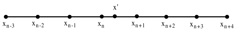
Figure 20: Illustration of Lagrangian interpolation.

C.1 Interpolation Options for GetVelocity and GetVelocityAndPressure

In this section, $f$ denotes any one of the three components of velocity, $u$, $v$ or $w$, or pressure, $p$, depending on which function is called. $\Delta x$, $\Delta y$ and $\Delta z$ are the width of grid in $x$, $y$ and $z$ direction. ${\bf x^{\prime}}=(x^{\prime},y^{\prime},z^{\prime})$.

NoSInt: No spatial interpolation

In this case, the value at the datapoint closest to each coordinate value is returned, rounding up or down in each direction.

$$f({\bf x^{\prime}}) = f(x_{n},y_{p},z_{q})$$ (28)

where $n=int(\frac{x^{\prime}}{\Delta x}+\frac{1}{2})$, $p=int(\frac{y^{\prime}}{\Delta y}+\frac{1}{2})$, $q=int(\frac{z^{\prime}}{\Delta z}+\frac{1}{2})$.

Lag4: 4th-order Lagrange Polynomial interpolation

In this case, 4th-order Lagrange Polynomial interpolation is done along each spatial direction.

$$f({\bf x^{\prime}}) = \sum_{i=1}^{4}\sum_{j=1}^{4}\sum_{k=1}^{4}f(x_{n-2+i},y_{p-2+j},z_{q-2+k})$$ (29)

$$\cdot l_{x}^{n-2+i}(x^{\prime})\cdot l_{y}^{p-2+j}(y^{\prime})\cdot l_{z}^{q-2+k}(z^{\prime})$$

$$l_{\theta}^{i}(\theta^{\prime}) = \frac{\prod\limits_{j=n-1,j\neq i}^{n+2}(\theta^{\prime}-\theta_{j})}{\prod\limits_{j=n-1,j\neq i}^{n+2}(\theta_{i}-\theta_{j})}$$ (30)

where $\theta$ can be $x$, $y$, or $z$.

Lag6: 6th-order Lagrange Polynomial interpolation

In this case, 6th-order Lagrange Polynomial interpolation is done along each spatial direction.

$$f({\bf x^{\prime}}) = \sum_{i=1}^{6}\sum_{j=1}^{6}\sum_{k=1}^{6}f(x_{n-3+i},y_{p-3+j},z_{q-3+k})$$ (31)

$$\cdot l_{x}^{n-3+i}(x^{\prime})\cdot l_{y}^{p-3+j}(y^{\prime})\cdot l_{z}^{q-3+k}(z^{\prime})$$

$$l_{\theta}^{i}(\theta^{\prime}) = \frac{\prod\limits_{j=n-2,j\neq i}^{n+3}(\theta^{\prime}-\theta_{j})}{\prod\limits_{j=n-2,j\neq i}^{n+3}(\theta_{i}-\theta_{j})}$$ (32)

where $\theta$ can be $x$, $y$, or $z$.

Lag8: 8th-order Lagrange Polynomial interpolation

In this case, 8th-order Lagrange Polynomial interpolation is done along each spatial direction.

$$f({\bf x^{\prime}}) = \sum_{i=1}^{8}\sum_{j=1}^{8}\sum_{k=1}^{8}f(x_{n-4+i},y_{p-4+j},z_{q-4+k})$$ (33)

$$\cdot l_{x}^{n-4+i}(x^{\prime})\cdot l_{y}^{p-4+j}(y^{\prime})\cdot l_{z}^{q-4+k}(z^{\prime})$$

$$l_{\theta}^{i}(\theta^{\prime}) = \frac{\prod\limits_{j=n-3,j\neq i}^{n+4}(\theta^{\prime}-\theta_{j})}{\prod\limits_{j=n-3,j\neq i}^{n+4}(\theta_{i}-\theta_{j})}$$ (34)

where $\theta$ can be $x$, $y$, or $z$.

C.2 Interpolation Options for GetVelocityGradient, GetPressureGradient, GetVelocityLaplacian, GetVelocityHessian and GetPressureHessian

In this section, $f$ denotes velocity or pressure gradient, velocity or pressure Hessian, or velocity Laplacian, depending on which function is called.

FD4NoInt, FD6NoInt, FD8NoInt: No spatial interpolation

In this case, the value of the 4th, 6th or 8th order finite-difference evaluation of the derivative at the datapoint closest to each coordinate value is returned, rounding up or down in each direction.

$$f({\bf x^{\prime}}) = f(x_{n},y_{p},z_{q})$$ (35)

where $n=int(\frac{x^{\prime}}{\Delta x}+\frac{1}{2})$, $p=int(\frac{y^{\prime}}{\Delta y}+\frac{1}{2})$, $q=int(\frac{z^{\prime}}{\Delta z}+\frac{1}{2})$.

FD4Lag4: 4th-order Lagrange Polynomial interpolation of the 4th-order finite differences

In this case, the values of the 4th order finite-difference evaluation of the derivative at the data points are interpolated using 4th-order Lagrange Polynomials.

$$f({\bf x^{\prime}}) = \sum_{i=1}^{4}\sum_{j=1}^{4}\sum_{k=1}^{4}f(x_{n-2+i},y_{p-2+j},z_{q-2+k})$$ (36)

$$\cdot l_{x}^{n-2+i}(x^{\prime})\cdot l_{y}^{p-2+j}(y^{\prime})\cdot l_{z}^{q-2+k}(z^{\prime})$$

$$l_{\theta}^{i}(\theta^{\prime}) = \frac{\prod\limits_{j=n-1,j\neq i}^{n+2}(\theta^{\prime}-\theta_{j})}{\prod\limits_{j=n-1,j\neq i}^{n+2}(\theta_{i}-\theta_{j})}$$ (37)

where $\theta$ can be $x$, $y$, or $z$.

Appendix D Documentation: Database Temporal Interpolation Options

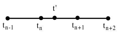
Figure 21: Illustration of data points for time.

In this section, $f$ denotes velocity, pressure, velocity or pressure gradient, velocity or pressure Hessian, or velocity Laplacian, depending on which function is called. $\Delta t$ is the time increment between consecutive times stored in the database.

NoTInt: No temporal interpolation

In this case, the value at the datapoint closest to the time value is returned, rounding up or down.

$$f(t^{\prime}) = f(t_{n})$$ (38)

where $n=int(\frac{t^{\prime}}{\Delta t}+\frac{1}{2})$.

PCHIP: Cubic Hermite Interpolation in time

The value from the two nearest time points is interpolated at time $t^{\prime}$ using Cubic Hermite Interpolation Polynomial, with centered finite difference evaluation of the end-point time derivatives - i.e. a total of four temporal points are used.

$$f(t^{\prime})=a+b(t^{\prime}-t_{n})+c(t^{\prime}-t_{n})^{2}+d(t^{\prime}-t_{n})^{2}(t^{\prime}-t_{n+1})$$ (39)

where

$$a = f(t_{n})$$

$$b = \frac{f(t_{n+1})-f(t_{n-1})}{2\Delta t}$$

$$c = \frac{f(t_{n+1})-2f(t_{n})+f(t_{n-1})}{2\Delta t^{2}}$$

$$d = \frac{-f(t_{n-1})+3f(t_{n})-3f(t_{n+1})+f(t_{n+2})}{2\Delta t^{3}}$$

References

- [1] J. Schumacher and K. R. Sreenivasan. Statistics and geometry of passive scalars in turbulence. Phys. Fluids 17:125107, 2005.
- [2] P. .K. Yeung Lagrangian investigations of turbulence. Annu. Rev. Fluid Mech 34:115?142, 2002.
- [3] A. Alexakis, P. D. Mininni and A. Pouquet Shell-to-shell energy transfer in magnetohydrodynamics. I. Steady state turbulence. Phys. Rev. E 72:046301, 2005.
- [4] NSF Cyberinfrastructure Council. Cyberinfrastructure vision for 21st century discovery. http://www.nsf.gov/pubs/2007/nsf0728/index.jsp, 2007.
- [5] A. S. Szalay, P. Z. Kunszt, A. Thakar, J. Gray, D. Slutz, and R. J. Brunner. Designing and mining mult-terabyte astronomy archives: the Sloan digital sky survey. Proceedings of the 2000 ACM SIGMOD international conference on Management of data, pages 451–462, 2000.
- [6] CINECA Supercomp. Center, iCFDdatabase; the CFD database http://cfd.cineca.it, examined July 2007.
- [7] DNSdb http://www.ae.gatech.edu/people/pyeung/DNSdb.html, examined March 2008.
- [8] S. Hoyas and J. Jimenez Scaling of the velocity fluctuations in turbulent channels up to . Phys. Fluids 18:011702, 2006.
- [9] E. Perlman, R. Burns, Y. Li, and C. Meneveau. Data exploration of turbulence simulations using a database cluster. SC07, 2007.
- [10] Y. Li and C. Meneveau. Origin of non-Gaussian statistics in hydrodynamic turbulence. Phys. Rev. Lett., 95:164502, 2005.
- [11] Y. Li and C. Meneveau. Intermittency trends and Lagrangian evolution of non-Gaussian statistics in turbulent flow and scalar transport. J. Fluid Mech., 558:133–142, 2006.
- [12] A. N. Kolmogorov. The local structure of turbulence in incompressible viscous fluid for very large Reynolds number. Dokl. Akad. Nauk. SSSR, 30:301–305, 1941.
- [13] U. Frisch. Turbulence: the legacy of A. N. Kolmogorov. Cambridge universtiy press, Cambridge, 1995.
- [14] S. B. Pope. Turbulent flows. Cambridge University Press, Cambridge, 2000.
- [15] R. Benzi, G. Paladin, G. Parisi, and A. Vulpiani. On the multifractal nature of fully developed turbulence and chaotic systems. J. Phys. A, 17:3521–3531, 1984.
- [16] C. Meneveau and K. R. Sreenivasan. Simple multifractal cascade model for fully developed turbulence. Phys. Rev. Lett., 59:1424–1427, 1987.
- [17] R. H. Kraichnan. Model of intermittency in hydrodynamic turbulence. Phys. Rev. Lett., 65:575–578, 1990.
- [18] Z.-S. She and E. Leveque. Universal scaling laws in fully developed turbulence. Phys. Rev. Lett., 72:336–339, 1994.
- [19] G. Falkovich, K. Gawedzki, and M. Vergassola. Particles and fields in fluid turbulence. Rev. Mod. Phys., 73:913–975, 2001.
- [20] L. Biferale. Shell models of energy cascade in turbulence. Annu. Rev. Fluid Mech., 35:441–468, 2003.
- [21] M. Chertkov, A. Pumir, and B. I. Shraiman. Lagrangian tetrad dynamics and the phenomenology of turbulence. Phys. Fluids, 11:2394–2410, 1999.
- [22] E. Jeong and S. S. Girimaji. Velocity-gradient dynamics in turbulence: Effect of viscosity and forcing. Theoret. Comput. Fluid Dynamics, 16:421–432, 2003.
- [23] L. Chevillard and C. Meneveau. Lagrangian dynamics and statistical geometric structure of turbulence. Phys. Rev. Lett., 97:174501, 2006.
- [24] F. van der Bos, B. Tao, C. Meneveau, and J. Katz. Effects of small-scale turbulent motions on the filtered velocity gradient tensor as deduced from holographic particle image velocimetry measurements. Phys. Fluids, 14:2456–2474, 2002.
- [25] B. J. Cantwell. Exact solution of a restricted Euler equation for the velocity gradient tensor. Phys. Fluids A, 4:782–793, 1992.
- [26] N. Z. Cao and S. .Y. Chen. Statistics and structures of pressure in isotropic turbulence. Phys. Fluids, 11:2235–2250, 1999.
- [27] G. S. Patterson and S. A. Orszag. Spectral calculations of isotropic turbulence: efficient removal of aliasing interactions. Phys. Fluids, 14:2538–2542, 1971.
- [28] http://www.w3.org/TR/soap/.
-
[29]
R. A. van Engelen.
gSOAP: SOAP C++ web services.
http://www.cs.fsu.edu/
~engelen/soap.html. - [30] http://turbulence.pha.jhu.edu/Service.asmx.
- [31] H. Lam and T. L. Thai. .NET framework essentials, 3rd Edition. O’Reilly, 2003.
- [32] H. Samet. Foundations of multidimensional and metric data structures. Morgan Kaufmann Publishers Inc., San Francisco, CA, USA, 2006.
- [33] H. Kang, S. Chester, and C. Meneveau. Decaying turbulence in an active-grid-generated flow and comparisons with large-eddy simulation. J. Fluid Mech., 480:129–160, 2003.
- [34] T. Gotoh, D. Fukayama, and T. Nakano. Velocity statistics in homogeneous steady turbulence obtained using a high-resolution direct numerical simulation. Phys. Fluids, 14:1065–1081, 2002.