PAIR PRODUCTION OF SCALAR TOP QUARKS IN POLARIZED PHOTON-PHOTON COLLISIONS AT ILC

Abstract

We study pair production of scalar top quarks (stop, $\tilde{t}_{1}$) in polarized photon-photon collisions with the subsequent decay of the top squarks into $b$-quarks and charginos $\tilde{t}_{1}\to b\tilde{\chi}_{1}^{\pm}$. We simulate this process by using PYTHIA6.4 for an electron beam energy $2E^{e}_{beam}=\sqrt{s_{ee}}=1000$ GeV. A set of criteria for physical variables is proposed which leads to a good separation of stop signal events from top quark pair production being the main background. These criteria allow us to reconstruct the mass of the top squark provided that the neutralino mass is known.

^a University of Vienna, Faculty of Physics, 1090 Vienna, Boltzmanngasse 5, Austria.
^b AHEP Group, Instituto de Fisica Corpuscular - C.S.I.C., Universidad de Valencia, Edificio Institutos de Investigacion, Apt. 22085, E-46071 Valencia, Spain
^c Institute for High Energy Physics (HEPHY Vienna), Nikolsdorfergasse 18, A-1050 Vienna, Austria.
^d DESY, Platanenallee 6, D-15738 Zeuthen, Germany.
^e JINR, Joliot-Curie 6, 141980 Dubna, Moscow region, Russia.

1 Introduction.

The scalar top quark, the bosonic partner of the top quark, is expected to be the lightest colored supersymmetric (SUSY) [1] particle. $\tilde{t}_{L}$ and $\tilde{t}_{R}$, the supersymmetric partners of the left-handed and right-handed top quarks, mix and the resulting two mass eigenstates $\tilde{t}_{1}$ and $\tilde{t}_{2}$, can have a large mass splitting. It is even possible that the lighter eigenstate $\tilde{t}_{1}$ could be lighter than the top quark itself [2], [3].

Searches for top squarks were performed at LEP and Tevatron and will continue at LHC and ILC [4], [5]. At ILC it is planned to have the option of a photon collider (PLC), as originally planned for TESLA [6]. This will be achieved by using backscattered photon beams by Compton scattering of laser photon beams with electron beams [7] - [15], (for recent review on this subject see [17]).

It has been stressed that the polarization effects in the interactions of backscattered laser photons [11]–[15] provide additional opportunities for studying the properties of the produced particles (see also [6] and [4], [5]). In the following we study the reaction

$$\gamma+\gamma\to\tilde{t}_{1}+\bar{\tilde{t}_{1}}.$$ (1)

Among the possible $\tilde{t}_{1}$-decay channels within the MSSM (see [18] for details), we focus on the decay $\tilde{t}_{1}\to b\tilde{\chi}_{1}^{\pm}$ followed by the two-body chargino decay $\tilde{\chi}_{1}^{\pm}\to\tilde{\chi}_{1}^{0}W^{\pm}$, where one of the W’s decays hadronically, $W\to q_{i}{\bar{q}_{j}}$, and the other one leptonically, $W\to\mu\nu_{\mu}$ [19] . The final state of this signal process, shown in the left plot of Fig.1, contains two $b$-quarks and two quarks (originating from thedecay of one W boson), a hard muon plus a neutrino (from the decay of the other W) and two neutralinos:

$$\gamma\gamma\to\tilde{t}_{1}\bar{\tilde{t}_{1}}\to b\bar{b}\tilde{\chi}^{+}_{1}\tilde{\chi}^{-}_{1}\to b\bar{b}W^{+}W^{-}\tilde{\chi}^{0}_{1}\tilde{\chi}^{0}_{1}\to b\bar{b}q_{i}\bar{q_{j}}\mu\nu_{\mu}\tilde{\chi}^{0}_{1}\tilde{\chi}^{0}_{1}.$$ (2)

The main background process is top quark pair production with the subsequent decay $t\to bW^{\pm}$ (for W’s we use the same decay channels as in the stop case):

$$\gamma\gamma\to t\bar{t}\to b\bar{b}W^{+}W^{-}\to b\bar{b}q_{i}\bar{q_{j}}\mu\nu_{\mu}.$$ (3)

The only difference between the final states of stop and top production (shown in the right diagram of Fig.1) is that the stop pair production has two neutralinos which are undetectable. Thus, both processes have the same signature: two $b$-jets, two jets from W decay and a muon. In the following we show that the physical variables constructed out of the final state may us allow to reconstruct the scalar top quark mass. In the present paper we consider only top pair production as background.

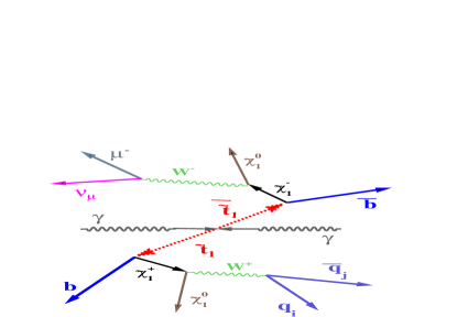
a) b)

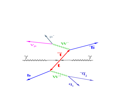
Figure 1: Left is the stop signal event diagram, Right is the top background diagram.

We analyse the processes (2) and (3) with the help of Monte Carlo samples of the corresponding events. Two programs PYTHIA6.4 [25] and CIRCE2 [26] were used. To simulate stop pair production process (1), we used the PYTHIA6.4 event generator in which the formula for the cross section of the stop pair production in $e^{+}e^{-}$ annihilation was replaced by the formula for two scalar particles (s) production $\gamma\gamma\to s\bar{s}$ from [27], [28], [16], (see [29] for the NLO corrections and [30] for more details about differential cross sections), which takes into account various photon polarization states. The top background was also simulated with PYTHIA6.4. The program CIRCE2 was used to generate the momentum spectra of the backscattered photons involved in the process (1). The energy of the electron beams was chosen to be $E_{beam}^{e}$ = 500 GeV (i.e. the total $e^{-}e^{-}$ energy is $E_{e-e-}^{tot}=\sqrt{s_{ee}}=1000$ GeV).

In Section 2 we give the set of MSSM parameters used in our study.

In Section 3 the important backscattered photon beam characteristics, namely, momentum spectra and luminosity, are considered for the case of polarized photon production in Compton scattering of polarized laser photons and polarized electrons.

In Section 4 we discuss some general characteristics of the signal process $\gamma\gamma\to\tilde{t}_{1}\tilde{\bar{t}}_{1}$ and the main background $\gamma\gamma\to t\bar{t}$. The subsections include kinematical distributions for the produced stop quarks, for the jets originating from W boson decay and for $b$-jets. We compare them in detail with those of top pair production. Subsection 4.2 also deals with the reconstruction of the invariant mass of the two-quark system stemming from the W boson decay as well as with the reconstruction of the invariant mass of the corresponding two-jet system. Subsection 4.3 contains the energy and transverse momentum spectra and some angular distributions of $b$-quarks and the corresponding $b$-jets. In Subsection 4.4 we demonstrate how to discriminate between the signal muons produced in W boson decays and those stemming from hadron decays in the same events.

In Section 5 we show the distributions of the global variables as missing energy, total visible (i.e. detectable) energy, the scalar sum of the transverse momenta of all visible particles in the event and the invariant mass of the final-state hadronic jets plus the signal muon. Two further global variables, the invariant mass of all final-state hadronic jets and the missing mass, are also introduced here. It is shown that they are very useful for the separation of background top events.

In Section 6 we propose three cuts which provide a good signal-to-background ratio (S/B).

Section 7 is devoted to the mass reconstruction of the scalar top quark based on the distribution of the invariant mass of one $b$-jet and the other two $non-b$-jets (from W decay), provided that the neutralino mass is known.

In Section 8 we show the distributions of the invariant variables described in Section 7 for a stop mass $M_{\widetilde{t}_{1}}=200$ GeV.

Section 9 contains some conclusions.

2 MSSM parameters and cross section.

The scalar top quark system is described by the mass matrix (in the $\tilde{t}_{L}-\tilde{t}_{R}$ basis) [2], [31]

$$\left(\begin{array}[]{cc}M^{2}_{\tilde{t}_{LL}}&M^{2}_{\tilde{t}_{LR}}\\ M^{2}_{\tilde{t}_{RL}}&M^{2}_{\tilde{t}_{RR}}\end{array}\right)$$ (4)

with

$$M^{2}_{\tilde{t}_{LL}}=M^{2}_{\tilde{Q}}+(\frac{1}{2}-\frac{2}{3}sin^{2}\Theta_{W})cos2\beta M^{2}_{Z}+M^{2}_{t},$$ (5)

$$M^{2}_{\tilde{t}_{RR}}=M^{2}_{\tilde{U}}+\frac{2}{3}sin^{2}\Theta_{W}cos2\beta M^{2}_{Z}+M^{2}_{t},$$ (6)

$$M^{2}_{\tilde{t}_{RL}}=(M^{2}_{\tilde{t}_{LR}})^{*}=M_{t}(A_{t}-\mu^{*}cot\beta).$$ (7)

The mass eigenvalues are given by

$$M^{2}_{\tilde{t}_{1,2}}=\frac{1}{2}\left[(M^{2}_{\tilde{t}_{LL}}+M^{2}_{\tilde{t}_{RR}})\mp\sqrt{(M^{2}_{\tilde{t}_{LL}}+M^{2}_{\tilde{t}_{RR}})+4|M^{2}_{\tilde{t}_{LR}}|}\right]$$ (8)

with the mixing angle

$$cos\Theta_{\tilde{t}}=\frac{-M^{2}_{\tilde{t}_{LR}}}{\sqrt{|M^{2}_{\tilde{t}_{LR}}|^{2}+(M^{2}_{\tilde{t}_{1}}-M^{2}_{\tilde{t}_{LL}})^{2}}}$$ (9)

$$sin\Theta_{\tilde{t}}=\frac{M^{2}_{\tilde{t}_{LL}}-M^{2}_{\tilde{t}_{1}}}{\sqrt{|M^{2}_{\tilde{t}_{LR}}|^{2}+(M^{2}_{\tilde{t}_{1}}-M^{2}_{\tilde{t}_{LL}})^{2}}}$$ (10)

In the following we shall consider only one particular choice of the MSSM parameters that are defined, in the notations of PYTHIA6, in the following way:

$\bullet$ $M_{\widetilde{Q}}=270$ GeV;
$\bullet$ $M_{\widetilde{U}}=270$ GeV;
$\bullet$ $A_{t}=-500$ GeV (top trilinear coupling);
$\bullet$ $tan\beta=5$;
$\bullet$ $\mu=-370$ GeV;
$\bullet$ $M_{1}=80$ GeV;
$\bullet$ $M_{2}=160$ GeV.

Note that in PYTHIA6 $M_{\widetilde{Q}}$ corresponds to $M_{\widetilde{t}_{L}}$ (left squark mass for the third generation) and $M_{\widetilde{U}}$ corresponds to $M_{\widetilde{t}_{R}}$. These parameters give $M_{\widetilde{t}_{1}}=167.9$ GeV, $M_{\chi^{+}_{1}}=159.2$ GeV and $M_{\chi^{0}_{1}}=80.9$ GeV. This parameter point is compatible with all experimental data. We have chosen this value of $M_{\widetilde{t}_{1}}$ to be rather close to the mass of the top quark $M_{t}=170.9\pm 1.8$ GeV [32]. Therefore, one expects a rather large contribution from the top background, which means that the choice of this value of the stop mass makes the analysis most difficult. Finding a suitable set of cuts separating stop and top events is therefore crucial.

3 Photon beam characteristics.

Let us mention two main features of photon-photon collisions. The first one is that the monochromaticity of the backscattered photon beam is considerably increased if the mean helicities $\lambda_{e}$ and $P_{c}$ of the electron beam and the laser photon beam are chosen such that $2\lambda_{e}P_{c}\approx-1$, as has been shown in [11]-[13] . In this case the relative number of hard photons becomes nearly twice as large in the region of the photon energy fractions $y_{i}=E_{i}^{\gamma}/E^{e}_{beam}\approx 0.7-0.85,$ i = 1, 2, where $E_{1,2}^{\gamma}$ are the energies of the two backscattered photon beams. Thereby the luminosity in collisions of these photons increases by a factor of 3-4. The growth of backscatterd photon energy spectra in the region of large $y_{i}$ with the increase of ($-2\lambda_{e}P_{c}$) is illustrated in Fig.3 of [11] and in Fig.2 of [13]. In other words, when ($-\lambda_{e}P_{c}$) increases, the effective ”pumping” of soft laser photons into hard backscattered ones increases due to the Compton process. The analogous growth of spectral luminosity $dL_{\gamma\gamma}/dW$ (W is the invariant mass of $\gamma\gamma$ system) in the case when the polarizations in both incoming systems of beam electron and the laser photon satisfy the relation $2\lambda_{1e}P_{1c}=2\lambda_{2e}P_{2c}$ is demonstrated in Figs.4 of [11] and [13]. As it was mentioned in [11], at $2\lambda_{e}P_{c}\approx-1$ the photons with the maximal energy ($y_{i}\approx 0.7-0.85$) are circular polarized and their helicity is close to ($-P_{c}$). Thus, in the limit $2\lambda_{1e}P_{1c}=2\lambda_{2e}P_{2c}=-1$, the produced pair of most energetic photons have total angular momentum J=0 or J=2, depending on the signs of $P_{1c}$ and $P_{2c}$. This allows one to measure the cross sections $\sigma_{0}$ and $\sigma_{2}$ which correspond to collisions of $\gamma\gamma$-pairs having total angular momentum 0 or 2, respectively.

The other feature stems from the fact that unlike the situation at an electron-positron collider, the energy of the beams of backscattered photons will vary from event to event. As already mentioned in the Introduction, we use the program CIRCE2 [26] for the energy spectra of the colliding backscattered photons, as well as the values of photon beam luminosities. CIRCE2 uses as input the data files that were generated for TESLA using the code and the set of beam parameters described in [33], [15] and [6] . We use as a reasonable approximation the CIRCE2 output spectra obtained on the basis of the above mentioned data files that were originally generated for $E_{e-e-}^{tot}=800$ GeV and scale them (by 1000/800) to the higher beam energy $2E^{e}_{beam}=E_{e^{-}e^{-}}^{tot}=1000$ GeV.

The photon energy spectrum obtained in this way without of any cuts with CIRCE2 for this total energy $E_{e^{-}e^{-}}^{tot}=1000$ GeV is shown in Fig.2 . Two peaks are clearly seen in this figure. The left one at a low photon energy is caused by multiple Compton scattering and beamstrahlung photons [14], [15], [33] and [6]. The second one, according to [10]-[13], appears in the region of hard photon production $y_{1,2}\approx 0.83$. It shows the degree of monochromaticity of the produced backscattered high–energy photons.

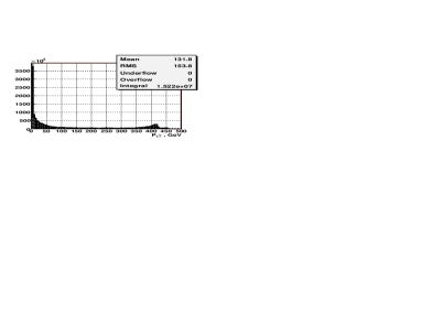
Figure 2: The whole photon momentum spectrum generated by CIRCE2.

The energy spectra of backscattered photons, as provided by CIRCE2, are used as input for PYTHIA for the generation of stop pair production events. Due to the stop pair mass threshold $2M_{\widetilde{t}_{1}}$, only in about $0.3\%$ of the CIRCE2 events the energy of produced backscattered $\gamma\gamma$-system is high enough for the generation of $\gamma\gamma\to\tilde{t}\tilde{\bar{t}}$ signal events by PYTHIA.

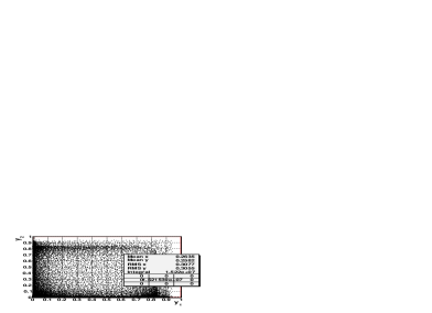
a) b)

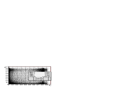
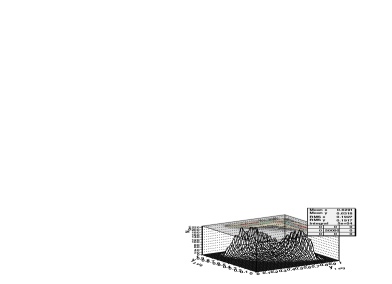
c) d)

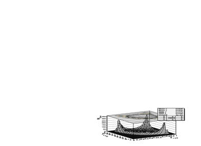
Figure 3: a) correlation spectra of the energy fractions $y_{1}$ and $y_{2}$ for events generated by CIRCE2 for the case of the opposite sign polarizations of backscattered photons (”J=2 case”). c) correlation spectrum for that part of the events shown in plot a) in which the energy of $\gamma\gamma$-system is above the threshold of stop pair production. b) and d) are the same correlation spectra as a) and c) spectra but obtained for the case of the same sign polarizations of backscattered photons (”J=0 case”). $E_{e^{-}e^{-}}^{tot}=1000$ GeV.

The correlations between the energies of two colliding photons given by CIRCE2 are shown in the plots a) and b) of Fig.3.

The two-dimensional plot a) in Fig.3 shows the correlation between the energy fractions of produced photons $y_{1}$ and $y_{2}$ for the case that the two colliding backscattered photons have opposite sign helicities, i.e. when the total helicity of $\gamma\gamma$-system $J=2$ . Plot b) is for $J=0$ i.e., it is for the case that the two colliding backscattered photons have the same sign helicities ⁵. The distribution in plot b) shows maxima at $y_{1,2}\approx 0.83$, which corresponds to the high-energy peak in Fig.2 and $2\lambda_{e}P_{c}\approx-1$. The number of generated events in the cases a) and b) are shown by the ”Integral” values in the statistic frames of both plots. They were chosen such to produce equal number (50000) of events at the PYTHIA level of simulation (see ”Integral” values in the plots c) and d)) of the two different samples of signal stop production events having different polarization states of the incoming $\gamma\gamma$ pairs.

The lower two plots c) and d) of Fig.3 are 3-dimensional plots with their projections onto the $y_{1}-y_{2}$ plane. They also show the correlations between the energy fractions $y_{1}$ and $y_{2}$ of the backscattered photons. In these plots we include only those events that lead to the production of a stop-antistop $\tilde{t}\bar{\tilde{t}}$ pair. The left side of Fig.3 shows the plots for the opposite sign polarization case (i.e., $J=2$) and the right side for the same sign polarization case (i.e., $J=0$). Plots b) and d) show the enhancement of the $J=0$ state contribution at $y_{1,2}\approx 0.83$.

It is worth mentioning that in a real photon-photon collision experiment none of these cases would appear in a pure form because of the unavoidable presence of some admixture of other photon polarization states .

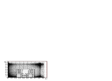
a) b)

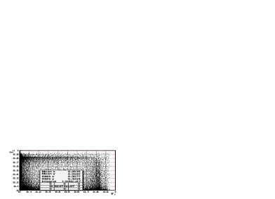
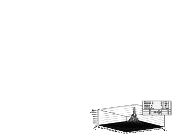
c) d)

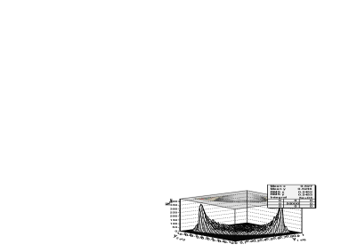
Figure 4: The same as in Fig.3 but with the $J=2$ state contribution enhanced.

The simultaneous change of the signs of the laser photon and beam electron helicities at only one side of the colliding beams does not change the equality $2\lambda_{1e}P_{1c}=2\lambda_{2e}P_{2c}$ [10]-[13], but leads to a different beam configuration, which may influence the shape of the luminosity spectrum. In Fig.4 we present the correlation plots that are analogous to those of Fig.3 but this time they are for the case of the above mentioned simultaneous sign reversal of the laser photon and electron beam polarizations at one side ($i=2$, for example) of the colliding beams. It is seen from the plots a) and c) that this combination gives an increase of the contribution of the two-photon system of total angular momentum $J=2$.

Finally we give the values of total photon-photon luminosities and the corresponding values of stop pair production cross sections (for the chosen value of the stop mass) obtained from CIRCE2 and PYTHIA6 for $E_{e-e-}^{tot}=1000$ GeV for the opposite sign (${+-~{}\&~{}-+}$) and the same sign (${++~{}\&~{}--}$) backscattered photon helicities :

$\bullet$ for the plots shown in Fig.3 (i.e., enhanced $J=0$ state)

$L^{\gamma\gamma}_{+-~{}\&~{}-+}$ = 9.35 * $10^{2}$ $fb^{-1}year^{-1}$ ;       $\sigma^{\tilde{t}_{1}\bar{\tilde{t}_{1}}}=2.91$ fb;

$L^{\gamma\gamma}_{++~{}\&~{}--}$ = 1.02 * $10^{3}$ $fb^{-1}year^{-1}$ ;       $\sigma^{\tilde{t}_{1}\bar{\tilde{t}_{1}}}=4.96$ fb.

$\bullet$ for the plots shown in Fig.4 (i.e., enhanced $J=2$ state).

$L^{\gamma\gamma}_{+-~{}\&~{}-+}$ = 1.02 * $10^{3}$ $fb^{-1}year^{-1}$ ;        $\sigma^{\tilde{t}_{1}\bar{\tilde{t}_{1}}}=6.13$ fb;

$L^{\gamma\gamma}_{++~{}\&~{}--}$ = 9.35 * $10^{2}$ $fb^{-1}year^{-1}$ ;        $\sigma^{\tilde{t}_{1}\bar{\tilde{t}_{1}}}=4.70$ fb.

4 Distributions of kinematical variables in stop and top production.

In this Section we present various plots for the kinematical distributions of different physical variables based on two samples of $2.5\cdot 10^{4}$ stop pair production events generated by CIRCE2 and PYTHIA6.4. They were weighted by the photon-photon luminosity calculated with the help of CIRCE2 and given above for the corresponding polarizations. Analogous plots are also given for $1.0\cdot 10^{5}$ generated background top events.

The generation of all events, i.e. for the stop and top production, was done separately for both possible combinations of photon polarizations, i.e. for the same sign ( $"++"$ and $"--"$) and for the opposite sign ($"+-"$ and $"-+"$) helicities.

In the following we present only those plots which correspond to the case where the relative alignment of laser photon and beam electron helicities enhances the contribution of the colliding two-photon system with the total angular momentum $J=0$ (i.e., corresponding to Fig.3).

To find the jets we use the subroutine PYCLUS of PYTHIA. The parameters of this jet finder are chosen such that the number of jets is exactly four.

4.1 Distributions in stop events.

Figures 5–8 show some general kinematical distributions characteristic of the produced stop pair system, i.e., the distributions of the energy of the stop or antistop $E_{\widetilde{t}_{1}}$, the transverse momentum $PT_{\widetilde{t}_{1}}$, the polar angle $\theta_{\widetilde{t}_{1}}$ (all in $e^{-}e^{-}$ c.m.s.) and the invariant mass of the produced stop pair $M_{inv}(\widetilde{t}_{1}+\bar{\widetilde{t}}_{1})$. In these plots we do not distinguish between stop and antistop. By comparing the left hand side of these figures with the right side one sees the effects of the different chosen polarizations (and corresponding luminosities).

In Fig.5 one can see that the stop energy $E_{\widetilde{t}_{1}}$ spectra start close to the value of the stop mass $M_{\widetilde{t}_{1}}=167.9$ GeV. In the case of opposite sign photon polarizations (plot a)) the spectrum has a peak at $E_{\widetilde{t}_{1}}\approx 320$ GeV and it is characterized by a high mean value $E_{\widetilde{t}_{1}}^{mean}=311$ GeV. It means that the produced stops are rather energetic. In the case of the same sign polarizations (plot b)) the energy spectrum is softer, having the main peak at $E_{\widetilde{t}_{1}}\approx 200$ GeV and the mean value about 274 GeV. So, one may expect that the stops produced in the same sign case are on the average less energetic than in the opposite sign case. One can also see a second smaller peak at $E_{\widetilde{t}_{1}}\approx 400$. This is due to the effect of the luminosity and cross section enhancement in the $J=0$ case at $y_{1}\approx y_{2}\approx 0.83$ (see the right-hand plots of Fig.3).

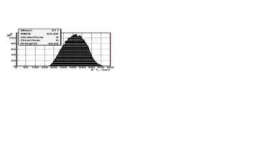
a) b)

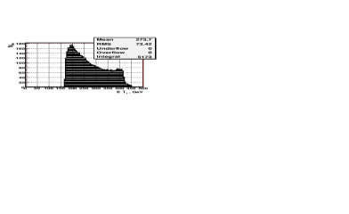
Figure 5: Stop energy $E_{\widetilde{t}_{1}}$ spectra. a) $"+-"$ and $"-+"$ polarizations, b) $"++"$ and $"--"$ polarizations.

Figure 6 shows analogous distributions for the stop transverse momentum $PT_{\widetilde{t}_{1}}$. The $PT_{\widetilde{t}_{1}}$ spectrum for the same sign polarizations (plot b)) is much softer than for the opposite sign polarizations (plot a)), with mean values of 111 GeV and 214 GeV, respectively.

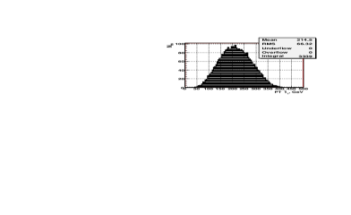
a) b)

Figure 6: Stop transverse momentum $PT_{\widetilde{t}_{1}}$ spectra. a) $"+-"$ and $"-+"$ polarizations, b) $"++"$ and $"--"$ polarizations.

The polar angle $\theta_{\widetilde{t}_{1}}$ distributions are shown in Fig.7. One can see that the distribution for $"+-"$ and $"-+"$ polarizations (plot a)) is very different from that for $"++"$ and $"--"$ polarizations (plot b)).

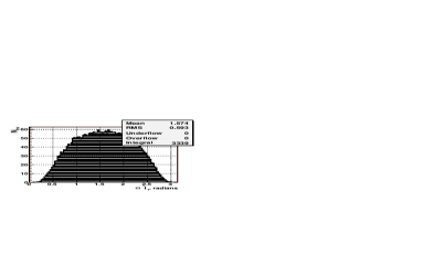
a) b)

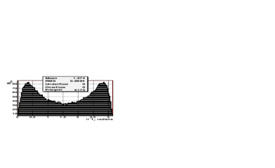
Figure 7: Stop polar angle $\theta_{\widetilde{t}_{1}}$ spectra. a) $"+-"$ and $"-+"$ polarizations, b) $"++"$ and $"--"$ polarizations.

The invariant mass $M_{inv}(\widetilde{t}_{1}+\bar{\widetilde{t}}_{1})$ spectra of the produced stop-antistop system are shown in Fig.8. For $"+-"$ and $"-+"$ polarizations (plot a)) it has a peak around 550 GeV, which is about 170 GeV higher than the analogous peak at 380 GeV for $"++"$ and $"--"$ polarizations (plot b)). Note that the shapes of the distributions of the invariant mass of the stop pairs shown in Fig.8 follow the energy spectra given in Fig.5. Thus, the second peak in plot b) of Fig.8 at $M_{inv}(\widetilde{t}_{1}+\bar{\widetilde{t}}_{1})\approx 800$ GeV has the same origin as the peak in the plot b) of Fig.5 at $E_{\widetilde{t}_{1}}\approx 400$ GeV.

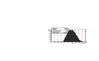
a) b)

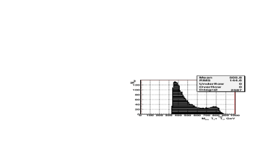
Figure 8: Stop pair invariant mass $M_{inv}(\widetilde{t}_{1}+\bar{\widetilde{t}}_{1}$) spectra. a) $"+-"$ and $"-+"$ polarizations, b) $"++"$ and $"--"$ polarizations.

The vertical axis in the plots shows the number of stops and antistops produced per year ($=10^{7}sec$) in each bin. Taking the integral of the distributions and dividing its value by two (there is one stop-antistop pair in each event) one can get the total number of events expected per year for the applied cuts. These numbers are shown as ”Integral” values within the statistical frames in the upper corners of the plots. They are calculated by taking into account the ratio of the photon-photon luminosity in the energy region above the stop pair threshold over the total photon-photon luminosity. In the case of $"+-"$ and $"-+"$ polarizations this ratio is approximately 0.419. From Fig.8 it is seen that the number of events per year for the $"++"$ and $"--"$ backscattered photon polarizations is equal to $N_{++/--}=2587$. It is appreciably larger than the corresponding number of events per year $N_{+-/-+}=1669$ for $"+-"$ and $"-+"$ polarizations.

4.2 Jet distributions from W decay.

According to the decay chain (2), the final state has to contain two jets due to the decay of one W boson into two quarks $W\to q_{i}+\bar{q}_{j}$ (see Fig.1).

Fig.9 shows the distributions of the energy $E_{W-quark}$ of the quarks produced in the W boson decay (which we call ”$W$-quarks”) for stop (plots a) and b)) and top (plots c) and d)) production. Plots a) and c) present $"+-"$ and $"-+"$ polarizations, while plots b) and d) present $"++"$ and $"--"$ polarizations. The stop-quark spectra begin at zero and go up to 220 GeV, with a mean values of $\approx 65$ GeV, while the top-quark spectra go up to approximately 300-350 GeV, with the mean values of 85-97 GeV.

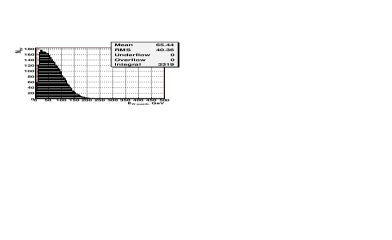
a) b)

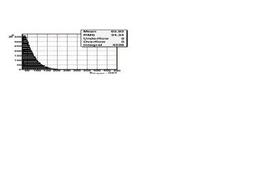
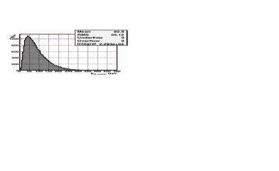
c) d)

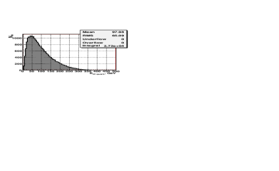
Figure 9: Energy spectra of the quarks from W boson decay. a) and b) are for the stop pair production; c) and d) are for the top pair production. a) and c) $"+-"$ and $"-+"$ polarizations, b) and d) $"++"$ and $"--"$ polarizations.

Fig.10 shows the transverse momentum $PT_{W-quark}$ spectra of the quarks produced in the W boson decay for stop (plots a) and b)) and top (plots c) and d)) production. Plots a) and c) are for $"+-"$ and $"-+"$ polarizations, plots b) and d) are for $"++"$ and $"--"$ polarizations. The shapes of the $PT_{W-quark}$ spectra of these ”$W$-quarks” are rather similar to the $E_{W-quark}$ spectra. In the case of top production the ”$W$-quarks” are slightly more energetic and have a larger transverse momentum than those from stop pair production.

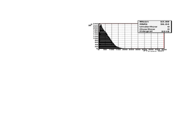
a) b)

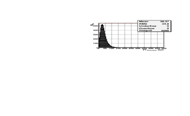
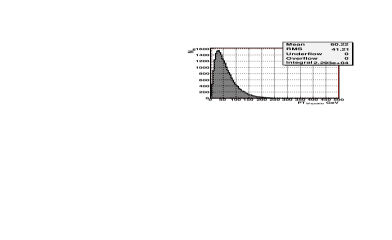
c) d)

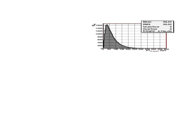
Figure 10: PT spectra of the quarks produced in the W boson decay. a) and b) are for the stop pair production; c) and d) are for the top pair production. a) and c) $"+-"$ and $"-+"$ polarizations, b) and d) $"++"$ and $"--"$ polarizations.

As the next step we take into account the hadronization of the ”$W$-quark” into a jet which we call ”$jet_{W}$”. Figs.11 and 12 show the energy $E_{jet_{W}}$ and transverse momentum $PT_{jet_{W}}$ distributions of the corresponding ”$W$-jets”. Plots a) and b) are for stop, plots c) and d) are for top production. Plots a) and c) present $"+-"$ and $"-+"$ polarizations, while plots b) and d) present $"++"$ and $"--"$ polarizations. According to our choice of PYCLUS jet finder parameters there are two ”$jet_{W}$” in the event.

a) b)

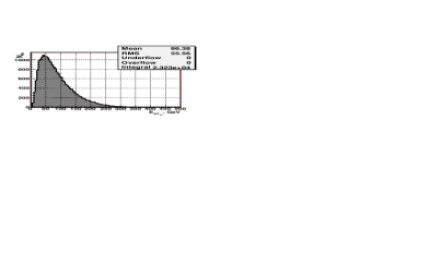
c) d)

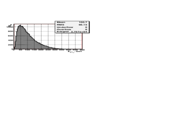
Figure 11: $E_{jet_{W}}$ energy spectra. a) and b) are for the stop pair production; c) and d) are for the top pair production. a) and c) $"+-"$ and $"-+"$ polarizations, b) and d) $"++"$ and $"--"$ polarizations.

Comparing plots a) and b) of Fig.11 for the energy distribution of ”W-jets” in stop production with the corresponding plots of Fig.9, one observes that the corresponding mean values of the ”W-jets” energy $E_{jet_{W}{*}}$ (we use the notation $W^{*}$ for the virtual W) in Fig.11 is about 19-25 GeV lower than the mean energy $E_{W-quark}$ of ”$W$-quarks”. It is also seen (Fig.9) that the peak positions of ”$W$-quark” energy distribution in the stop case ($E^{peak}_{W-quark}\approx 25$ GeV) is shifted to the left by about 15 GeV ($E^{peak}_{jet_{W}{*}}\approx 10$ GeV) when passing to the jet level (see plots a) and b) of Fig.11). The end point of the $E_{jet_{W}{*}}$ distribution in the stop case is somewhat lower than that for the corresponding quarks.

Analogously, the mean values and the peak positions of the distribution of the transverse momentum the ”$W^{*}$-quarks” $PT_{W^{*}-quark}$, shown in Fig.10 a) and b), decrease by about 12-20 GeV when passing to the jet level (see Fig.12 a) and b)), while the end point of the $PT_{jet_{W}{*}}$ distribution is a bit lower than the end point of $PT_{W^{*}-quark}$ distribution.

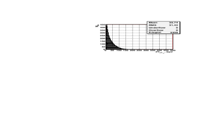
a) b)

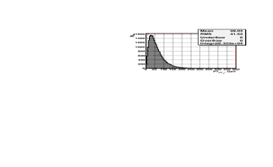
c) d)

Figure 12: ”$jet_{W}$” PT- spectra. a) and b) are for the stop pair production; c) and d) are for the top pair production. a) and c) $"+-"$ and $"-+"$ polarizations, b) and d) $"++"$ and $"--"$ polarizations.

Due to the different kinematics in top production mentioned above, the spectrum of the the energy $E_{jet_{W}}$, its peak position and the mean value of the ”$jet_{W}$” energy distribution in the top case are practically equivalent to the $E_{W-quark}$ spectrum, peak position and the mean value of the corresponding ”$W$-quark” energy distribution (see Fig.9 c), d) and Fig.11 c), d)). Analogously, by comparing plots c) and d) of Figs.10 and 12 for $PT_{W-quark}$ and $PT_{jet_{W}}$, one can see that the transverse momentum distribution in top production is stable under hadronization.

Figure 13 shows the spectrum of the invariant mass $M_{W}=M_{inv}(quark1+quark2)$ reconstructed from the vectorial sum of 4-momenta of the two ”W-quarks”. The main features of these plots practically do not differ for $"+-"$ and $"-+"$ and the $"++"$ and $"--"$ polarization cases. Therefore we do not show them separately. Plot a) is for stop pair production, plot b) is for top production. In plot a) of Fig.13 one clearly sees the virtual nature of the W boson in the stop pair production case. Hence, in the stop case the invariant mass of two quarks produced in the decay of the virtual W boson ($W^{*}$) is smaller than the mass of a real W boson. In top production (see plot b) of Fig.13) there is a peak in the invariant mass distribution at the mass value of the real W boson.

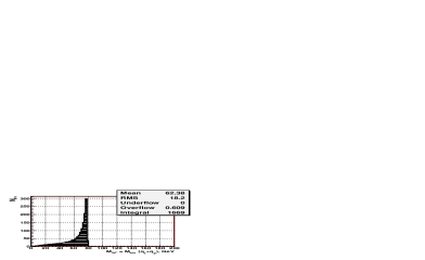
a) b)

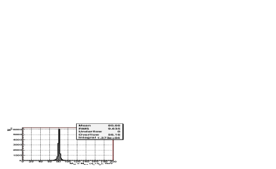
Figure 13: The invariant mass of two quarks $M_{W}=M_{inv}(quark1+quark2)$, reconstructed from the vectorial sum of 4-momenta of two quarks that are produced in $W\to q_{i}+\bar{q}_{j}$ decay. a) stop pair production; b) top pair production.

Figure 14 shows the corresponding plots at the jet level. The invariant mass is built

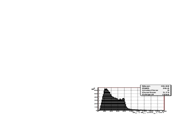
a) b)

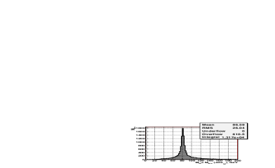
Figure 14: Number of generated events versus the reconstructed invariant mass of ”all-non-$b$-jets”. a) stop pair production; b) top pair production.

of ”all-non-$b$-jets” (or, shortly, “$jets_{W^{*}}$”). One can see from plot a) that in the stop case the peak position of $M_{inv}(jets_{W^{*}})$ is shifted to the left and a long tail for higher invariant masses appears. As seen from plot b), in the top case at the jet level the position of the W-peak remains at the same value of $M_{W}$ (with a high precision) as in plot b) of Fig.13, except some shifting of the mean value. From comparison of plots a) and b) of Fig.14 we conclude that the cut $M_{inv}(jets_{W^{*}})\leq 70$ GeV may allow us to eliminate this tail and a big amount of the top background.

4.3 $b$-quark and $b$-jet distributions in stop and top production.

In the case of stop decay into a $b$-quark and a chargino, $\tilde{t}_{1}\to b\tilde{\chi}_{1}^{\pm}$, the jets produced in $b$-quark hadronization are observable objects. Their features are interesting from the viewpoint of experimentally distinguishing the stop signal events from the top background.

In Fig.15 we show in plots a) and b) the distributions of the energies $E_{b}$ of the $b$- and $\bar{b}$-quarks (which we do not distinguish in the following) produced in the decay $\tilde{t}_{1}\to b\tilde{\chi}_{1}^{\pm}$ for the $"+-"$, $"-+"$ and $"++"$, $"--"$ polarizations, respectively. Both spectra begin at $E_{b}\approx 4$ GeV, corresponding to the b-quark mass, and go up to $E_{b}\approx 34$ GeV. The mean values are about 14 GeV and 13 GeV, respectively. Plots c) and d) of Fig.15 are two analogous plots for top pair production. The corresponding spectrum in top production is much harder and its main part is concentrated within the interval $45<E_{b}<150$ GeV. The mean values are $E_{b}\approx 113$ GeV and $E_{b}\approx 130$ GeV, respectively, which is almost four times higher than the end point of the $b$-jet energy spectra in the stop events. It means that in the stop case the b-quark takes a smaller part of the stop energy than the b-quark gets in the background top case.

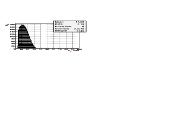
a) b)

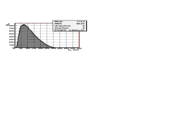
c) d)

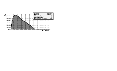
Figure 15: $b$- and $\bar{b}$-quark energy spectra. a) and b) are for the stop pair production; c) and d) are for the top pair production. a) and c) $"+-"$ and $"-+"$ polarizations, b) and d) $"++"$ and $"--"$ polarizations.

Figure 16 shows the transverse momentum $PT_{b}$ spectra of $b$-quarks for stop (plots a) and b)) and top (plots c) and d)) production. Plots a) and c) are for $"+-"$ and $"-+"$ polarizations, plots b) and d) are for $"++"$ and $"--"$ polarizations. Comparing the distributions in Figs.15 and 16 with the corresponding ones in Figs.5 and 6, one can conclude that in stop pair production the $b$-quarks have only a small fraction of the energy and transverse momentum of the parent stops. The shape of the $PT_{b}$ spectra of $b$-quarks in the stop case is similar to the shape of the $E_{b}$ spectra. This means that in the stop decay the transverse component of the $b$-quark momentum is larger than the longitudinal component.

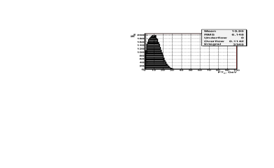
a) b)

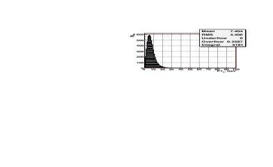
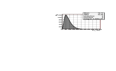
c) d)

Figure 16: b- and $\bar{b}$-quark PT spectra. a) and b) are for the stop production; c) and d) are for the top case. a) and c) $"+-"$ and $"-+"$ polarizations, b) and d) $"++"$ and $"--"$ polarizations.

The kinematical distributions of the $b$-quarks in top decay are quite different. The $b$-quarks produced in top decays are very energetic. Most of the top events have $E_{b}\geq 25$ GeV and $PT_{b}\geq 20$ GeV. The difference to stop decay is easily understandable. The stop decays into a heavy chargino, whereas the top decays into a real W boson whose mass is only half of the mass of the chargino $M_{\chi_{1}^{\pm}}$. Therefore, the $b$-quarks in top decays have a larger phase space than the $b$-quarks in stop decays.

The distribution of the polar angle $\Theta_{b}$ of the $b$-quarks in stop production are presented in Fig.17. Plot a) is for $"+-"$ and $"-+"$ polarizations, plot b) is for $"++"$ and $"--"$ polarizations. The difference between these distributions due to the polarization effects is clearly seen in this figure.

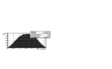
a) b)

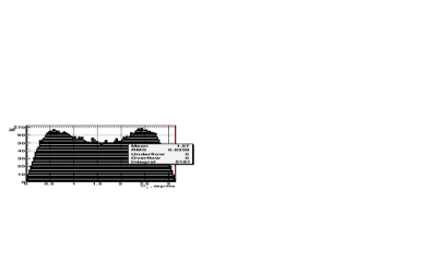
Figure 17: The spectra of the b- and $\bar{b}$-quark polar angle $\theta_{b}$ for stop production events. a) $"+-"$ and $"-+"$ polarizations, b) $"++"$ and $"--"$ polarizations.

In Fig.18 the $cos(b,\bar{b})$ distribution is shown, where $cos(b,\bar{b})$ is the cosine of the opening angle between the 3-momenta of the $b$- and $\bar{b}$-quarks produced in the same stop event. Plot a) is for $"+-"$ and $"-+"$ polarizations, plot b) is for $"++"$ and $"--"$ polarizations. It demonstrates that most of the $b$- and $\bar{b}$-quarks move in approximately opposite directions, but some are in the same hemisphere. Thus, in the experiment we may expect a similar angular distribution of the corresponding $b$- and $\bar{b}-jets$.

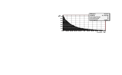
a) b)

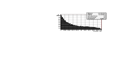
Figure 18: The spectra of $cos(b,\bar{b})$ for stop production events. a) $"+-"$ and $"-+"$ polarizations, b) $"++"$ and $"--"$ polarizations.

As the next step, we take into account $b$-quark hadronization into a $b$-jet. Fig.19

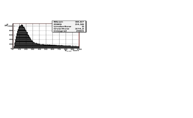
a) b)

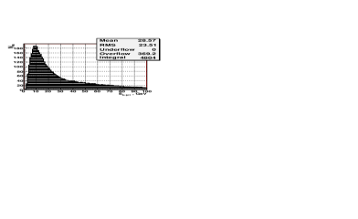
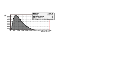
c) d)

Figure 19: b-jet energy spectra. a) and b) are for stop par production; c) and d) are for top par production. a) and c) $"+-"$ and $"-+"$ polarizations, b) and d) $"++"$ and $"--"$ polarizations.

shows the energy $E_{b-jet}$ distributions of the corresponding $b$-jets. Plots a) and b) of Fig.19 are for stop production and plots c) and d) are for top production. These and the following plots for jets are obtained using the distance measure of the ”Durham algorithm” implemented in the PYCLUS jet finder of PYTHIA. Technically, $b$-jets are defined as jets that contain at least one B-hadron. Their decay may be identified by the presence of a secondary vertex [37].

Comparing the upper plots a) and b) of Fig.19 for the $b$- and $\bar{b}$- jet energy distributions in stop production with the upper plots a) and b) of Fig.15 for the $b$-quark and $\bar{b}$-quark energy distributions, one observes the appearance of long tails at higher energies. One sees that the end points of the energy distributions for the $b$-jets and $\bar{b}$-jets are higher than those for the corresponding quarks. Furthermore, the corresponding mean values of the jet energies $E_{b-jet}$ in Fig.19 are about 15 GeV higher than those in Fig.15. It is interesting to note that the peak positions of the energy distributions $E_{b-jet}$ in the stop case shown in the plots a) and b) of Fig.19 for the $b$- and $\bar{b}$- jets practically coincide with those shown in the plots a) and b) of Fig.16 for $b$-quarks.

At the same time, due to the different kinematics in top production, the mean values of the $b$-jet and $\bar{b}$-jet energy distributions $E_{b-jet}$ in the top case are only by about 2 GeV smaller than the mean values of the corresponding $b$-quark and $\bar{b}$-quark energy distributions (see plots c) and d) in Fig.15 and Fig.19).

Figure 20 shows the transverse momentum $PT_{b-{jet}}$ distributions of the $b$-jets and $\bar{b}$-jets in stop production (plots a) and b)) and top production (plots c) and d)). By comparing with Fig.16 for the corresponding PT distributions at the $b$-quark level we can see, in analogy with the energy distributions, long tails at high PT which increase the mean PT values for stop production by about 15 GeV for $"+-"$ and $"-+"$ polarizations and by about 13 GeV for $"++"$ and $"--"$ polarizations. Note that the peak positions of the PT distributions shown in the plots a) and b) at the jet level practically do not differ from the positions of the peaks at the quark level (see plots a) and b) of Fig.16).

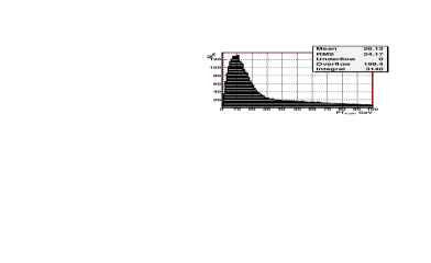
a) b)

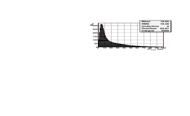
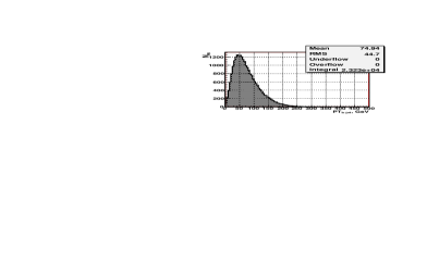
c) d)

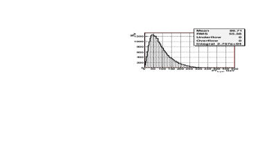
Figure 20: b-jet PT spectra. a) and b) are for stop pair production; c) and d) are for top pair production. a) and c) $"+-"$ and $"-+"$ polarizations, b) and d) $"++"$ and $"--"$ polarizations.

It is also seen that in the case of top production the mean values of the PT distributions of the $b$-jets practically do not differ from the analogous ones shown in the plots c) and d) of Fig.16 for $b$-quarks.

Let us summarize the results which were obtained in subsections 4.2 and 4.3 by the use of PYCLUS jet finder. First, it was found that in the case of top background production the characteristic parameters of energy and transverse momentum distributions of jets stemming from W decay and of $b$-jets, produced in $b$-quark hadronization, practically do not differ from the parameters of their parent quarks distributions.

This picture changes quite noticeably when we consider the case of stop production with its further decay through the channel $\tilde{t}_{1}\to b\tilde{\chi}_{1}^{\pm}$. In this case the $b$-quarks are essentially less energetic than the b-quarks produced in top decay $t\to bW^{\pm}$. The simulation has shown that the usage of the same PYCLUS jet finder in stop case leads to a noticeable redistribution of the jet energies between ”W-jets” and $b$-jets and, correspondingly, of jet transverse momenta. Namely, in the stop case the mean values of the jet energy $E_{jet_{W}{*}}$ and jet transverse momentum $PT_{jet_{W^{*}}}$ are about 12-25 GeV smaller than the energy $E_{W-quark}$ and transverse momentum $PT_{W-quark}$ of parent ”$W$-quarks” stemming from W boson decay. On the contrary, the mean values of the $b$-jet energy $E_{b-jet}$ and the jet transverse momentum $PT_{b-{jet}}$ are about 5-15 GeV higher than the energy $E_{b}$ and $PT_{b}$ of the parent $b$-quarks.

It is worth emphasizing that the positions of the peak of the energy and transverse momentum distributions are stable when going from the quark to the jet level. In the following we shall return to this subject and consider the set of physical variables which will take into account the effect of energy redistribution in the case of stop production.

4.4 Distributions of the signal muons.

To select the signal stop pair production events, see the left plot of Fig.1, one has to identify the muon from the W decay. The corresponding energy $E_{sig-mu}$ and transverse momentum $PT_{sig-mu}$ distributions of the signal muons are shown in Fig.21 for both polarization combinations.

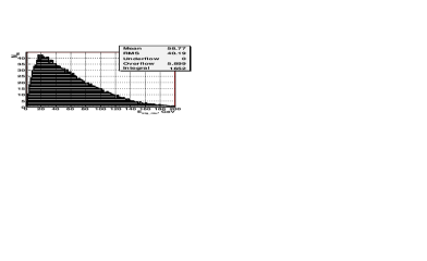
a) b)

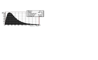
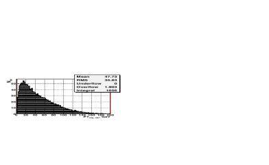
c) d)

Figure 21: Energy and PT distributions of signal muons. a) and c) $"+-"$ and $"-+"$ polarizations, b) and d) $"++"$ and $"--"$ polarizations.

There are, however, also muons in the event coming from leptonic and semileptonic decays of hadrons. The left and right plots of Fig.22 show the energy $E_{dec-mu}$ and the transverse momentum $PT_{dec-mu}$ spectra of these muons stemming from hadron decays within the detector volume, for which we took the size parameters from [4], [5]. It can be seen that the decay muons have a rather small energy $E_{dec-mu}$ and transverse momentum $PT_{dec-mu}$. Their mean values are about $0.85$ and $0.59$ GeV, respectively. The analogous spectra for the signal muons in Fig.21 show that the signal muons have a much higher energy $E_{sig-mu}$ and transverse momentum $PT_{sig-mu}$. The mean value of the signal muons energy $E^{mean}_{sig-mu}=47.6$ GeV is about 60 times higher than the mean value of the energy of the decay muons. An analogous difference can be seen between the mean values of transverse momenta PT of signal and decay muons. Therefore one can cut off most low–energy decay muons rejecting those with $E_{mu}\leq 6$ GeV. Such a cut leads to a loss of about $2\%$ of signal events as seen from the Fig.21 (the bin width in this plot is 2 GeV).

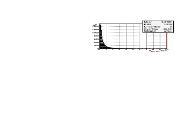
a) b)

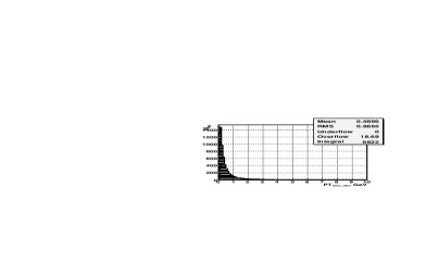
Figure 22: Distributions muons from leptonic and semileptonic decays. a) Energy distribution; b) PT distribution.

We have also studied another way to select the signal muon from W decay. If the axes of all four jets in the event are known, then in general the signal muon has the largest transverse momentum with respect to any of these jet axes.

5 Some global variables.

In stop pair production the two neutralinos and the energetic neutrino from the W boson decay escape detection. The simulation with PYTHIA6 allows us to estimate the missing energy and the missing transverse momenta that are carried away by these particles. We also take into account the non-instrumented region around the beam pipe given by the polar angle intervals $\Theta<7^{o}$ and $\Theta>173^{o}$.

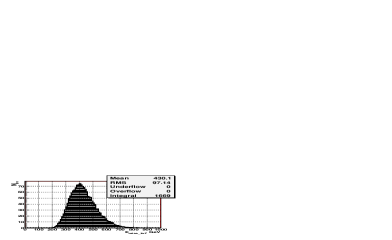
a) b)

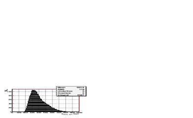
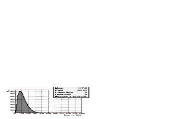
c) d)

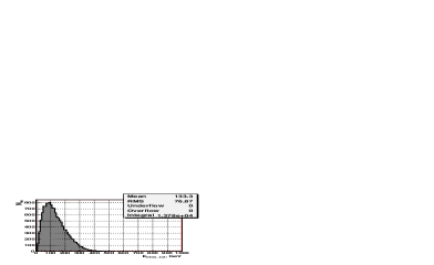
Figure 23: Missing energy $E_{miss-tot}$ distribution. a) and b) are for stop pair production; c) and d) are for top pair production. a) and c) $"+-"$ and $"-+"$ polarizations, b) and d) $"++"$ and $"--"$ polarizations.

The distributions of the total missing energy for stop production and top production are presented in the upper and lower plots of Fig.23, respectively. In stop pair production, see plots a) and b), the $E_{miss-tot}$ spectrum starts at 190-200 GeV and at ends 800 GeV. In top pair production (plots c) and d)), where the two neutralinos are not present, the missing energy $E_{miss-tot}$ is much smaller. It starts from $\approx 10$ GeV and finishes at $\approx 380-420$ GeV.

Figure 24 shows the distributions of the total visible energy in event $E_{vis-tot}$ in stop production (plots a) and b)) and in top production (plots c) and d)). The large missing energy in stop production (Fig.23) is related to the low visible energy (Fig.24), while in top production the low missing energy correlates with the large visible energy. A cut on the total visible energy of approximately $E_{vis-tot}<250$ GeV would eliminate most of the top background while approximately 10$\%$ of the signal events are lost.

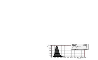
a) b)

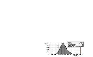
c) d)

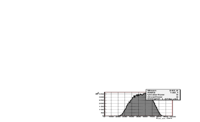
Figure 24: Total energy $E_{vis-tot}$ distribution. a) and b) are for stop pair production; c) and d) are for top pair production. a) and c) $"+-"$ and $"-+"$ polarizations, b) and d) $"++"$ and $"--"$ polarizations.

Another useful observable is the scalar sum of the moduli of the transverse momenta in an event $PT_{scalsum}=\sum\nolimits_{i=1}^{N_{part_{i}}}|PT_{i}|$, where the sum goes over all ($N^{part}$) detectable particles (i) in the event. Fig.25 shows the distributions of the scalar sum of the transverse momenta for stop production (plots a) and b)) and for top production (plots c) and d)). It is seen that the restriction $PT_{scalsum}\leq 180$ GeV would lead to a good separation of the stop signal events from the top background.

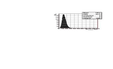
a) b)

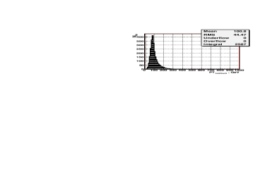
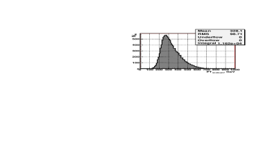
c) d)

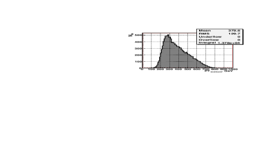
Figure 25: $PT_{scalsum}$ distribution. a) and b) are for stop pair production; c) and d) are for top pair production. a) and c) $"+-"$ and $"-+"$ polarizations, b) and d) $"++"$ and $"--"$ polarizations.

We consider also the invariant mass $M_{inv}(Alljets,\mu)$ of the system that contains all observable objects in the final state. This invariant mass is the modulus of the vectorial sum of the 4-momenta $P^{i}_{jet}$ ($N^{jet}=4,i=1,2,3,4$) of all four jets in an event plus the 4-momentum of the signal muon

$$M_{inv}(Alljets,\mu)=\sqrt{(\Sigma_{i=1,2,3,4}P^{i}_{jet}+P_{\mu})^{2}}~{}.$$ (11)

The distribution of this invariant mass is shown in Fig.26. Plots a) and b) show the results for stop pair production while the plots c) and d) are for top pair production. As seen from these plots, the cut $M_{inv}(Alljets,\mu)\leq 230$ GeV will give a good separation of signal stop and top background events.

a) b)

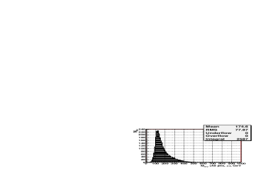
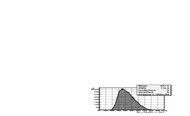
c) d)

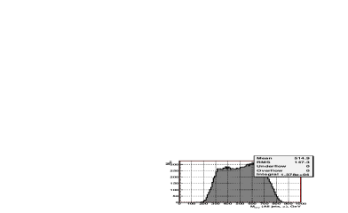
Figure 26: Distribution of number of events versus the reconstructed invariant mass of all jets and signal muon $M_{inv}(Alljets,\mu)$. a) and b) are for stop production; c) and d) are for top case. a) and c) $"+-"$ and $"-+"$ polarizations, b) and d) $"++"$ and $"--"$ polarizations.

Another variable that can also be used for the separation of the signal and the background is the ”missing” mass $M_{missing}$ (for $\sqrt{s}=\sqrt{s_{ee}}=1000$ GeV)

$$M_{missing}=\sqrt{(\sqrt{s}-(\sum\nolimits_{i=1}^{N^{jet}}{E^{i}_{jet}+E_{\mu}))^{2}}-(\sum\nolimits_{i=1}^{N^{jet}}{{\bf P}^{i}_{jet}+\bf P_{\mu})^{2}}}$$ (12)

This variable takes into account the contribution of those particles that cannot be registered in the detector (neutrinos and neutralinos). The distributions of this invariant ”missing” mass are given in Fig.27. Plot a) and b) show the results for stop pair production, while plots c) and d) are for top pair production. As seen from these plots, the cut $M_{missing}\geq 700$ GeV also allows us to get rid of most of the background.

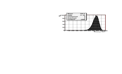
a) b)

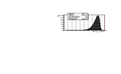
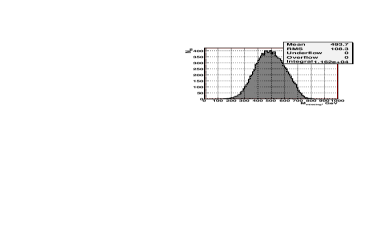
c) d)

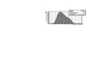
Figure 27: Distribution of number of events, versus the missing mass variable $M_{missing}$. a) and b) are for stop pair production; c) and d) are for top pair production. a) and c) $"+-"$ and $"-+"$ polarizations, b) and d) $"++"$ and $"--"$ polarizations.

An even more efficient separation of the signal and the background can be obtained by using the invariant mass $M_{inv}(Alljets)$ of the system that contains all jets.

$$M_{inv}(Alljets)=\sqrt{(\Sigma_{i=1}^{N^{jet}}P^{i}_{jet})^{2}}.$$ (13)

The corresponding distributions for the signal stop events (upper plots) and for the background top events (lower plots) are shown in Fig.28. It is seen that the application of the cut $M_{inv}(Alljets)\leq 180$ GeV leads to a practically complete separation of signal stop and top background events.

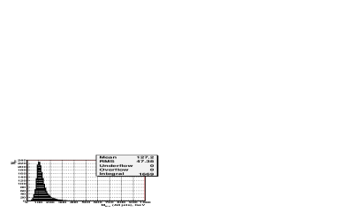
a) b)

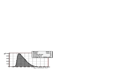
c) d)

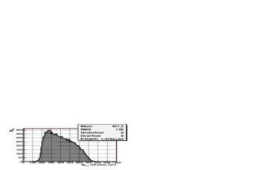
Figure 28: Distribution of number of events versus the reconstructed invariant mass of all jets $M_{inv}(Alljets)$. a) and b) are for stop pair production; c) and d) are for top pair production. a) and c) $"+-"$ and $"-+"$ polarizations, b) and d) $"++"$ and $"--"$ polarizations.

6 Cuts and signal-to-background ratio.

To diminish the influence of the jet energy redistribution effect, discussed in subsections 4.2 and 4.3, we shall use the cuts considered above for the $E_{vis-tot}$ and $M_{inv}(Alljets)$. These variables, by definition, include the total 4-momentum of all jets, defined as the vectorial sum of the 4-momenta of all jets. Therefore they do not suffer on energy redistribution between jets. Based on our results above, we will use the following three cuts to separate the signal and background events:

$\bullet$ there must be at least two $b$-jets in an event:

$$N_{b-jets}\geq 2;$$ (14)

$\bullet$ the invariant mass of all jets must be less than $180$ GeV:

$$M_{inv}(Alljets)\leq 180~{}GeV.$$ (15)

$\bullet$ the detected energy $E_{vis-tot}$ must be less than $250$ GeV:

$$E_{vis-tot}\leq 250~{}GeV;$$ (16)

All the figures presented in this paper are obtained after applying the first cut in order to get the right picture of jets when the $b$-jets are clearly determined.

These three cuts for the case with $J=0$ enhanced state considered here improve the signal–to–background ratio in the case of $"+-"$ and $"-+"$ polarizations from $S/B=0.15$ to $S/B\approx 60$, losing about $23.7\%$ (from 1903 to 1453) of the signal stop events and reduction of background top events from 1.227$\cdotp 10^{4}$ to 24. In the case of $"++"$ and $"--"$ polarizations an improvement of the signal–to–background ratio is from $S/B=0.222$ to $S/B\approx 123$, with a loss about $27.6\%$ (from 3233 to 2338) of the signal stop events and a reduction of the background top events from 1.441$\cdotp 10^{4}$ to 19.

Finally, we present the efficiency values for the three cuts (13)-(15). We define them as the summary efficiencies. It means that if $\varepsilon_{1}$ is the efficiency of the first cut (13), $\varepsilon_{12}$ is the efficiency of applying the first cut (13) and then the second cut (14). Analogously, $\varepsilon_{123}$ is the efficiency of the successive application of the cuts (13), (14) and (15).

$\bullet$ For SIGNAL STOP events :

$"+-"\&"-+"$ polarizations -     $\varepsilon_{1}=0.88$ ;      $\varepsilon_{12}=0.78$ ;      $\varepsilon_{123}=0.78$ ;

$"++"\&"--"$ polarizations -     $\varepsilon_{1}=0.80$ ;      $\varepsilon_{12}=0.73$ ;      $\varepsilon_{123}=0.72$ ;

$\bullet$ For BACKGROUND TOP events :

$"+-"\&"-+"$ polarizations -      $\varepsilon_{1}=0.94$ ;      $\varepsilon_{12}=0.011$ ;      $\varepsilon_{123}=0.002$ ;

$"++"\&"--"$ polarizations -      $\varepsilon_{1}=0.94$ ;      $\varepsilon_{12}=0.007$ ;      $\varepsilon_{123}=0.001$ .

7 Determination of the scalar top quark mass.

Another variable of interest is the invariant mass $M_{inv}$($b-jet$, $Jets_{W}$):

$$M_{inv}(b-jet,Jets_{W})\equiv\sqrt{(P_{b-jet}+P_{Jets_{W}})^{2}},$$ (17)

which is constructed as the modulus of the vectorial sum of the 4-momentum $P_{b-jet}$ of the $b$-jet, plus the total 4-momentum of $Jets_{W}$ system, i.e., non-$b$-jets stemming from the W decay ($P_{Jets_{W}}=P_{jet1_{W}}+P_{jet2_{W}}$, as there are only two jets allowed to be produced in W decay). More precisely, if the signal event contains a $\mu^{-}$ as the signal muon (see Fig.1), we have to take the $b$-jet ($\bar{b}$-jet in the case of $\mu^{+}$ as the signal muon). This is only possible if one can discriminate between the $b$- and $\bar{b}$-jets experimentally. Methods of experimental determination of the charge of the $b$-jet ($\bar{b}$-jet) were developed in [39]. In this paper we do not use any b-tagging procedure. The PYTHIA information about quark flavor is taken for choosing the $b$- and $\bar{b}$-jets. In reality, according to [39], a $50\%$ efficiency of the separation of $b$-jets and $80\%$ of the corresponding purity can be expected.

The distributions of the invariant masses of the ”$b$-jet+$Jets_{W}$” system in the case of stop pair production are shown in plots a) and b) of Fig.29 for the two polarization combinations, as well as in the case of top pair production in plots c) and d). Their analogs $M_{inv}(b,2~{}quarks_{W})$, obtained at quark level, are presented in Fig.30. The distributions shown in both Figures were obtained without use of cuts (15) and (16).

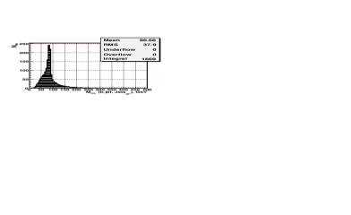
a) b)

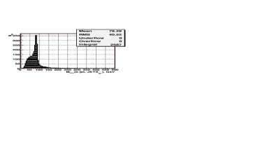
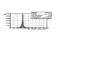
c) d)

Figure 29: The spectra of the invariant masses $M_{inv}$($b-jet$, $Jets_{W}$) obtained without use of cuts (15) and (16). a) and b) are for stop pair production; c) and d) are for top pair production. a) and c) $"+-"$ and $"-+"$ polarizations, b) and d) $"++"$ and $"--"$ polarizations.

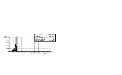
a) b)

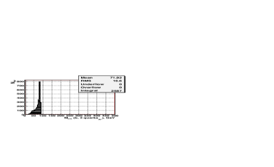
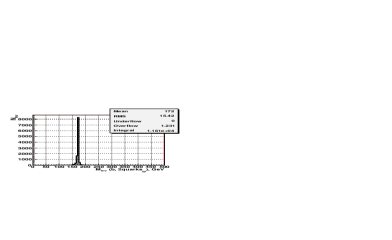
c) d)

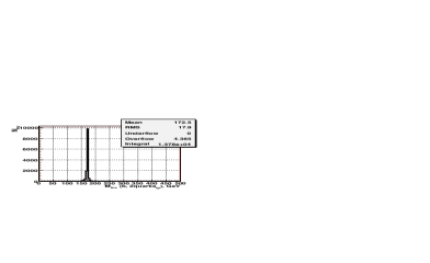
Figure 30: The spectra of the invariant masses $M_{inv}$($b$, $2~{}quarks_{W}$) obtained without use of cuts (15) and (16). a) and b) are for stop pair production; c) and d) are for top pair production. a) and c) $"+-"$ and $"-+"$ polarizations, b) and d) $"++"$ and $"--"$ polarizations.

In the top case the invariant mass $M_{inv}(b,2~{}quarks_{W})$ of the system composed of a $b$-quark and two quarks from W decay should reproduce the mass of their parent top quark (see Fig.1). The distributions of events $dN^{event}/dM_{inv}/5$ GeV expected in each bin of 5 GeV versus the invariant mass $M_{inv}(b,2~{}quarks_{W})$ of the parent three quarks as well as the invariant mass of jets produced by these quarks, i.e. $M_{inv}(b-jet,Jets_{W})$, are shown for jet and quark levels in plots c) and d) of Fig.29 and 30, respectively, for both polarizations. These distributions have an important common feature. Namely, they show that the peak positions at jet level and at quark level, practically coincide to a good accuracy with each other as well as with the input value of the top quark mass $M_{top}=170.9(\pm 1.8)$ GeV. It is also seen from Fig.29 that the quark hadronization into jets leads to a broadening of very small tails which are seen in the invariant mass distribution at quark level (Fig.30). The right tails, which appeared at jet level (see Fig.29), is a bit lower than the left tails and are longer than the left ones. One may say that the peak shape at jet level still looks more or less symmetric. The main message from these plots is that the appearance of tails due to quark fragmentation into jets does not change the position of the peak, which allows us to reconstruct the input top mass both at quark and jet levels.

An analogous stability of the peak position at the jet and quark levels for the stop case can be seen in the plots a) and b) of Figs.29 and 30. Note that, according to the stop decay chain (2), the right edge of the peak of the invariant mass distribution of the ”$b+2quarks_{W}$” system corresponds to the mass difference $M_{\widetilde{t}_{1}}-M_{\tilde{\chi}^{0}_{1}}$.

The distributions of the invariant mass of the ”$b+2quarks_{W}$” system (plots a) and b)) and of the invariant mass of the ”$b$-jet+$JETS_{W}$” system in the case of stop pair production are shown in Fig.31. Thereby only those stop events are taken that pass the cuts (14)–(16).

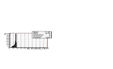
a) b)

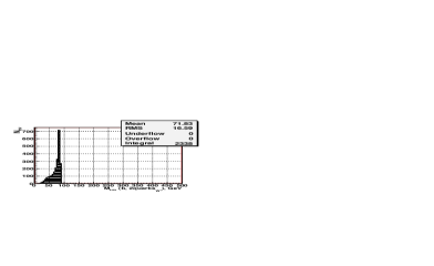
c) d)

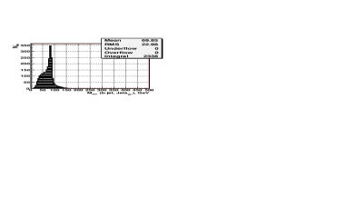
Figure 31: The spectra of the stop invariant masses after the cuts (14)–(16): a) and b) $M_{inv}$($b$, $2~{}quarks_{W}$); c) and d) $M_{inv}$($b-jet$, $Jets_{W}$). a) and c) $"+-"$ and $"-+"$ polarizations, b) and d) $"++"$ and $"--"$ polarizations.

Let us recall that according to Section 6 the application of the cuts (14)–(16) leaves only 24–19 background top events (respectively, for $"+-"$, $"-+"$ and $"++"$, $"--"$ combinations of photon polarizations) and saves about 76.3 $\%$ of signal stop events. It means that the distributions shown in plots c) and d) of Fig.29 would change drastically and resemble a random distribution of the 24–19 top events in a rather wide interval. The corresponding plots c) and d) of top production events which pass the cuts (14)–(16) are are made with a much larger simulated statistics and are shown in Fig.32. One sees that the surviving background top events will be mostly distributed in the region $30\leq M_{inv}$($b$-jet, $Jets_{W}$)$\leq 180$ GeV. This region is by more than twenty times wider than the 5 GeV width of the peak intervals in the $M_{inv}$($b$-jet, $Jets_{W}$) distributions which are shown in the stop plots c) and d) of Fig.31 (at jet level) and which contain about 240 (for $``+-``$ and $``-+``$ polarization) and 350 (for $``++``$ and $``--``$ polarization) signal stop events left after the cuts. Based on the shape of the distributions shown in the plots c) and d) of Fig.32 we can expect that in future measurements the contribution of these 24-19 remaining top background events will not influence the position of the peak of the $M_{inv}$($b$-jet, $Jets_{W}$) distributions (shown in plots c) and d) of Fig.31) which allow one to reconstruct the input value of the stop mass at jet level by adding the mass of the neutralino.

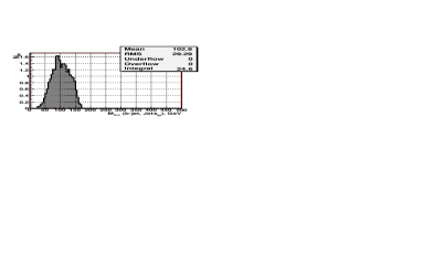
c) d)

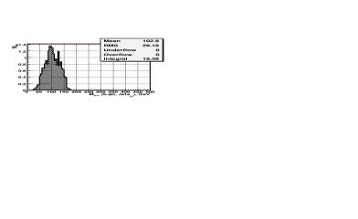
Figure 32: The spectra of the invariant mass $M_{inv}$($b$, $2~{}quarks_{W}$) for top pair production events after the cuts (14)–(16). a) $"+-"$ and $"-+"$ polarizations, b)$"++"$ and $"--"$ polarizations.

It is seen that the peak positions of the stop distribution at jet level $M_{inv}(b$-jet, $Jets_{W^{*}})$, obtained after the cuts (14)–(16) (plots c) and d) of Fig.31), coincide with the peak positions at quark level (plots a) and b) of Fig.31) as well as with the peak positions in plots a) and b) of Figs.29 and 30 obtained without any cuts. Let us note that the observed stability of the peak position in both of Figs.29 a), b) and 31 c), d) is due to the rather moderate loss of the number of events in the peak region (this loss is about 200 events) after cuts. The cuts lead (as it can be seen by comparing the mentioned plots) to a reduction of the right hand side tails of $M_{inv}(b$-jet, $Jets_{W^{*}})$ distributions.

Some additional remarks about the tails in the stop distributions are in order now. The origin of the right and left tails of the distributions, shown in the plots a) and b) of Fig.32, can be clarified by the results of the stop mass reconstruction by calculating its invariant mass at quark level $M_{inv}$($b$, $2~{}quarks_{W^{*}},\tilde{\chi}^{0}_{1})$ as the modulus of the sum of the 4-momenta of all three quarks and the neutralino (see Fig.1) in stop decay. These results are given in plots a) and b) of Fig.33 which shows a very precise reconstruction of the input stop mass at quark level withing the 5 GeV width of the bin containing the peak. Comparing plots a) and b) of Fig.31 with plots a) and b) of Fig.33 one can conclude that at quark level the long left tail as well as the very small right tail in the distribution of $M_{inv}$($b$, $2~{}quarks_{W^{*}})$ disappear when the neutralino 4-momentum is added to the 4-momentum of the ”$b+2quarks_{W}$” system.

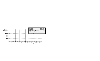
a) b)

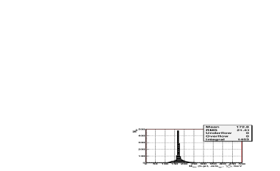
c) d)

Figure 33: The spectra of the invariant masses $M_{inv}$($b$-quark, $2~{}quarks_{W^{*}},\tilde{\chi}^{0}_{1})$, and $M_{inv}$($b$-jet, $Jets_{W},\tilde{\chi}^{0}_{1}$). a) and b) are for quarks level; c) and d) are for jets level. a) and c) $"+-"$ and $"-+"$ polarizations, b) and d) $"++"$ and $"--"$ polarizations.

The influence of the effect of the hadronization of the $b$-quarks and of the quarks from W decay into jets is shown in plots c) and d) of Fig.33. These plots demonstrate that the hadronization of quarks into jets practically does not change the positions of the stop mass peak, which practically concides with the input value $M_{\widetilde{t}_{1}}=167.9$ GeV. It is also seen that the hadronization results in the appearance of more or less symmetrical and rather suppressed short tails around the peak position. The mean values of the distributions in plots c) and d) of Fig.33 are slightly different from the mean values of the quark level distributions shown in plots a) and b) of Fig.33 but the peak positions remain the same. It is easy to see from plots c) and d) of Fig.31 that adding the mass of the neutralino $M_{\tilde{\chi}^{0}_{1}}=80.9$ GeV to the value of the right edge point of the peak $M_{inv}$($b$-jet, $Jets_{W*})\approx$ 85.2 GeV one can get the left lower limit for the reconstructed stop mass $M^{reco-low}_{\widetilde{t}_{1}}\approx 166.2$ GeV which reproduces well the input value $M_{\widetilde{t}_{1}}=167.9$ GeV.

Taking into account the bin width of 5 GeV used in the invariant mass distributions we may conclude that the method of the stop mass reconstruction based on the peak positions will be quite useful.

8   Results for top squark mass $M_{\widetilde{t}_{1}}$ = 200 GeV.

In this section we want to discuss what will change if the mass of the top squark is different from the one we have used before. In the present paper we have chosen a rather low scalar top quark mass (one of the lowest stop quark’s masses that is allowed for the case of $\tilde{t}_{1}\to b\tilde{\chi}_{1}^{\pm}$ decay channel). With increase of the stop mass the cross section for its production is decreasing. So, for example, for the case of $M_{\widetilde{t}_{1}}=200$ GeV the number of events per year is decreasing to 329 for the case of $"+-"$ and $"-+"$ polarizations and 1333 for the case of $"++"$ and $"--"$ polarizations (after the cuts (14)–(16)). The mass $M_{\widetilde{t}_{1}}=200$ GeV is still below the highest allowed stop mass for the $\tilde{t}_{1}\to b\tilde{\chi}_{1}^{\pm}$ decay channel (which is about 255 GeV) corresponding to $M_{\chi^{+}_{1}}=159.2$ GeV and $M_{\chi^{0}_{1}}=80.9$ GeV. For stop masses below and above the described region, the stop will decay to other channels which we do not consider in this paper.

The distribution of the invariant mass $M_{inv}$($b-jet$, $Jets_{W*}$) of the ”$b$-jet+$Jets_{W^{*}}$” system for events which have passed the cuts (14)–(16) is shown in Fig.34. Plot a) is for $"+-"$ and $"-+"$ polarization, b) is for $"++"$ and $"--"$ polarization. The top background also remains the same as it was given in Fig.32.

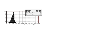
a) b)

Figure 34: The spectra of the invariant masses $M_{inv}$($b_{jet}$,$Jets_{W}$) of the ”$b$-jet+(all- non-$b$-jets)” system after cuts for $M_{\widetilde{t}_{1}}=200$ GeV. a) stop pair production; b) top pair production.

The distributions in Fig.34 have peaks at $M_{inv}$($b-{jet}$,$Jets_{W^{*}})\approx$ 110 GeV. One can also determine the mass of the stop quark following the procedure described in Section 7, but with less accuracy than in the case of the lower stop mass used in previous Sections.

9 Conclusion.

We have studied stop pair production in photon-photon collisions within the framework of the MSSM for the total energy of the $e^{-}e^{-}$ system $E_{e-e-}^{tot}=\sqrt{s_{ee}}=1000$ GeV. We assume that the stop quark decays dominantly into a chargino and a $b$-quark, $\tilde{t}_{1}\to b\tilde{\chi}_{1}^{\pm}$, and the chargino decays into a neutralino and a W boson, $\tilde{\chi}_{1}^{\pm}\to\tilde{\chi}_{1}^{0}W^{\pm}$, where the W boson is virtual. One of the two W’s decays hadronically, $W^{+}\to q\bar{q}$, the other one leptonically, $W^{-}\to\mu^{-}\nu$.

The study is based on a Monte Carlo simulation with two programs. First we have used the program CIRCE2 which gives the luminosity and the energy spectrum of the colliding backscattered photon beams. The results of CIRCE2 are taken as input for PYTHIA6.4. This event generator is used to simulate stop ($M_{\widetilde{t}_{1}}=167.9$ GeV) pair production and decay as well as top pair production being the main background.

Three cuts (14)-(16) have been proposed. The second (15) and the third (16) cut are the most important for the separation of the signal stop events from the background top events. They restrict the value of the invariant mass of all four jets (produced in $\gamma\gamma\to\tilde{t}_{1}\bar{\tilde{t}_{1}}\to b\bar{b}q_{i}\bar{q_{j}}\mu\nu_{\mu}\tilde{\chi}^{0}_{1}\tilde{\chi}^{0}_{1}$ process) and the value of the detected energy. This set of cuts leads to a signal–to–background ratio as large as $S/B=60$ in the case of the $"+-"$ and $"-+"$ polarizations and $S/B=123$ in the case of the $"++"$ and $"--"$ polarizations. Thus, we expect about $1-2\%$ admixture of top events to the stop signal. This is different from the more complicated situation in stop pair production at LHC (see, for instance, [38]).

We have shown that determining the end point of the peak in the distribution of the invariant mass $M_{inv}$($b$-jet,$Jets_{W^{*}}$) of the ”$b$-jet + two jets from W decay” system allow us to reconstruct the mass of the stop quark with a good accuracy based on the statistics of about two years running. For this the mass of $\tilde{\chi}_{1}^{0}$ has to be known.

We discussed the difference in the main invariant mass distributions for a mass $M_{\tilde{t}_{1}}$ = 200 GeV.

In conclusion, we can say that the $\gamma\gamma$ channel is very well suited for the study of stop pair production.

10 Acknowledgements.

This work is supported by the JINR-BMBF project and by the ”Fonds zur F$\ddot{o}$rderung der wissenschaftlichen Forschung” (FWF) of Austria, project No.P18959-N16. The authors acknowledge support from EU under the MRTN-CT-2006-035505 and MRTN-CT-2004-503369 network programmes. A.B. was supported by the Spanish grants SAB 2006-0072, FPA 2005-01269 and FPA 2005-25348-E of the Ministero de Educacion y Ciencia.

References

-
[1]
Y.Gol’fand and E.Likhtman, JETP Lett.13(1971) 323;
D.Volkov and V.Akulov, Phys.Lett. B46(1973) 109;
J.Wess and B.Zumino, Nucl.Phys. B70(1974) 39. - [2] J.Ellis and S.Rudaz, Phys.Lett. B128(1983) 248.
-
[3]
G.Altarelli and R.Rckl, Phys.Lett. B144(1984) 126;
S.Dawson, E.Eichten and C.Quigg, Phys.Rev. D31(1985) 1581;
K.Hikasa and M.Kobayashi, Phys.Rev. D36(1987) 742;
M.Drees and K.Hikasa, Phys.Lett. B252(1990) 127;
J.Ellis, G.L.Fogli and E.Lisi, Nucl.Phys. B393(1993) 3. -
[4]
ILC Reference Design Report, v.1 ”Executive Summary”,
Editors: J.Brau, Y.Okada, N.Walker, 2007;
http://www.linearcollider.org/cms/?pid=1000025. -
[5]
ILC Reference Design Report, v.2 ”Physics at the ILC”,
Editors: A.Djouadi, J.Lykken, K.Mnig, Y.Okada, M.Oreglia, S.Yamashita, 2007; http://www.linearcollider.org/cms/?pid=1000025. - [6] B.Badelek et al. ”TESLA Technical Design Report, PART VI: Appendices, Chapter 1: The Photon Collider at TESLA”, Editor V.Telnov, DESY, 2001; arXiv:hep-ex/0108012.
- [7] I.F.Ginzburg, G.L.Kotkin, V.G.Serbo, and V.I.Telnov, Preprint INP 81-50, Novosibirsk, 1981; JETP Lett. 34(1982)491.
- [8] C.Akerlof, ”Using the SLC as a Photon Accelerator”, Preprint UM HE 81-59, Univ. of Michigan, 1981 (unpublished).
- [9] I.F.Ginzburg, G.L.Kotkin, V.G.Serbo and V.I.Telnov, Preprint INP 81-102, Novosibirsk, 1981; Nucl. Instrum. Meth., A 205(1983)47.
- [10] I.F.Ginzburg, G.L.Kotkin, S.L.Panfil, V.G.Serbo and V.I.Telnov, Preprint INP 82-160, Novosibirsk, 1982.
- [11] I.F.Ginzburg, G.L.Kotkin, V.G.Serbo and V.I. Telnov, Sov.Jour. Nucl. Phys. 38, v.2 (1983) 372
- [12] I.F.Ginzburg, G.L.Kotkin, S.L.Panfil, V.G.Serbo, Sov. Jour. Nucl. Phys. 38, v.10 (1983)1021.
- [13] I.F.Ginzburg, G.L.Kotkin, S.L.Panfil, V.G.Serbo and V.I. Telnov, Nucl. Instrum. Meth., A 219(1984)5.
- [14] V.I.Telnov, Nucl. Instrum. Meth., A294(1990)72.
- [15] V.I.Telnov, Nucl. Instrum. Meth., A355(1995)3.
- [16] I.F.Ginzburg, Nucl. Instrum. Meth., A355(1995)63.
- [17] F.Bechtel et.al, Nucl. Instrum. Meth. A564(2006) 243; arXiv:physics/0601204.
- [18] A.Bartl, H.Eberl, S.Kraml, W.Majerotto and W.Porod, EPJ C2(2000)6; hep-ph/0002115.
- [19] A.Bartl, K.Moenig, W.Majerotto, A.Skachkova, N.Skachkov, ”Stop pair production in polarized photon-photon collisions”, Proc. of the Intern. Conf. on Linear Colliders (LCWS 2004), vol.II, p.919, April 19-23, 2004, Le Carre des Sciences, Paris, France.
- [20] A.Finch, H.Nowak and A.Sopczak, hep-ph/0211140.
- [21] M.Carena et. al, Phys.Rev. D72:115008, 2005; hep-ph/0508152.
- [22] A. Sopczak et. al, hep-ph/0605225.
- [23] A.Bartl, K.Moenig, W.Majerotto, A.Skachkova, N.Skachkov, Phys.Part.Nucl.Lett.6:181-189,2009.(No.3); arXiv:0906.3805 [hep-ph].
- [24] A.Bartl, K.Moenig, W.Majerotto, A.Skachkova, N.Skachkov, ”Pair production of scalar top quarks in e+e- collisions at ILC”; arXiv:0804.2125 [hep-ph].
- [25] T. Sjstrand, S.Mrenna, P.Skands, JHEP 05(2006) 026, hep-ph/0603175, LU TP 06-13, FERMILAB-PUB-06-052-CD-T.
-
[26]
T. Ohl,
http://theorie.physik.uni-wuersburg.de/ohl/circe2/circe2.ps;
http://theorie.physik.uni-wuerzburg.de/ohl/circe2/manual004.html. - [27] I.F.Ginzburg, V.G.Serbo, In Proc. of Winter School of LINP, vol.2, p.132, 1988.
- [28] I.F.Ginzburg, ”Physical Potential of Photon-Photon and Electron-Photon Colliders in Tev Region.” In Proc. IX Intern. Workshop on Photon-Photon Collisions, San Diego, CA, USA, 1992, p.474, Editors D.Caldwell and H.Paar, World Scientific.
- [29] S. Berge, “Gluino and squark pair production at future linear colliders.” DESY-THESIS-2003-048, Dec.2003, 106p.
- [30] S. Berge, M. Klasen, Y. Umeda, Phys.Rev. D63:035003, 2001.
- [31] J.F.Gunion, H.E.Haber, Nucl.Phys. B272(1986)1; B278(1986)449; Erratum B402(1993)567.
- [32] E.Brubaker et al., ”Combination of CDF and D0 results on the mass of the top quark”; By Tevatron Electroweak Working Group, Fermilab-TM-2380-E, 19 Mar2007; arXiv:hep-ex/0703034.
- [33] V. Telnov, hep-ph/001201.
- [34] T.Takahashi, K.Yokoya, V.I.Telnov, M.Xie, and K.Kim, Proc. of Snowmass Workshop, 1996.
- [35] P.Chen, T.Ohgaki, A.Spitkovski, T.Takahashi, and K.Yokoya. Nucl. Instrum. Meth., A397(1997)458; physics/9704012.
- [36] G.Klamke and K.Mnig, Eur.Phys.J. C42(2005)261, DESY-05-049, Mar 2005, hep-ph/0503191.
- [37] R.Hawkings, ”Vertex detector and flavour tagging studies for TESLA liear collider”, LC-PHSM-2000-021, 2000
-
[38]
U.Dydak, ”Search for the stop quark with CMS at
the LHC”; CMS TN/96-022, CERN, 1996;
U.Dydak, H.Rohringer and J.Tuominiemi, ”Study of the channel gluino stop + top”, CMS TN/96–103, CERN, 1996. -
[39]
C.J.S.Damerell, D.J.Jackson, eConf960625 (1996) DET078;
R.Hawkings, LC-PHSM-2000-021;
S.M.Xella Hansen, D.J.Jackson, R.Hawkings, C.J.S.Damerell, LC-PHSM-2001-024;
S.M.Xella Hansen, M.Wing, D.J.Jackson, N. De Groot, C.J.S.Damerell, LC-PHSM-2003-061;
S.M.Xella Hansen et. al. [Linear Collider Flavour Identification Collaboration], Nucl.Instrum.Meth. A501,106(2003); S.Hillert, C.J.S.Damerell, eConf0508141 (2005) ALCPG 1403. - [40] R.Hawkings, ”Vertex detector and flavour tagging studies for TESLA liear collider”, LC-PHSM-2000-021, 2000.