An efficient strategy to characterize alleles and complex haplotypes using DNA-markers

Abstract

We consider the problem of detecting and estimating the strength of association between a trait of interest and alleles or haplotypes in a small genomic region (eg a gene or a gene complex), when no direct information on that region is available but the values of neighbouring DNA-markers are at hand. We argue that the effects of the non-observable haplotypes of the genomic regions can and should be represented by factors representing disjoint groups of marker-alleles. A theoretical argument based on a hypothetical phylogenetic tree supports this general claim.

The techniques described allow to identify and to infer the number of detectable haplotypes in the genomic region that are associated with a trait. The methods proposed use an exhaustive combinatorial search coupled with the maximization of a version of the likelihood function penalized for the number of parameters. This procedure can easily be implemented with standard statistical methods for a moderate number of marker-alleles.

Key-words: Generalized Linear Models (GLIM), phylogenetic-tree, Akaike-information, Genetic-association, MHC

1 Introduction

Often in genetic applications, and in special in immune-genetics, interest lies in detecting and quantifying the association of a given genomic region to a trait. Here the genomic region might be a gene or a gene-complex. Typically, no bio-molecular or genomic information is directly available about this genomic region, but instead, a system of DNA-markers located close to the region is used. An example of this situation is the study presented by Schou et al, (2007, 2008) where the possible association of the susceptibility to several parasites and the major histocompatibility complex (MHC) in chickens was investigated using the microsatellite LEI0258 as a marker. Another example involves the use of a tight system of SNP markers to associate putative alleles in the MHC region and susceptibility to psoriasis in humans (Orru et al, 2002).

The association between alleles or haplotypes in the genomic region of interest and the trait is commonly characterized by a regression-like statistical model in which the trait enters as the dependent variable and factors representing the presence of the marker-alleles are included among the explanatory variables. A common practice is to declare association between the trait and the genomic region when at least one of the parameters representing the marker-alleles is statistically significant.

In order to establish association between traits and putative haplotypes in the genomic region of interest it is required to use a representation of those haplotypes in terms of marker-alleles (the only genomic information available). This representation is crucial to properly characterize the association. We argue that such a representation should be constructed with groups of marker-alleles instead of only individual marker alleles. Informally, our main point is that when considering only groups consisted of single marker-alleles (as usually done when using a naive approach) one might fail to represent alleles or haplotypes in the neighbouring genomic region. This leads to a significant reduction of efficiency or even to the complete loss of the capacity to detect certain associations. Our approach requires the use of a more complex statistical inference involving a search in a large number of possibilities. We show however, that the statistical inference is feasible for a moderate number of marker-alleles (10-15 allele-markers).

The text is organized as follows. Section 2 contains the basic setup, including a description of the genetic and molecular biological scenario, a formulation of the statistical model in terms of a generalized linear model and some discussion on the proper form of performing inference under those premises. A phylogenetic based argument justifying our proposal is presented in the last part of section 2. The details of the implementation of the statistical inference are given in section 3 and one examples is discussed in section 4. Some discussion is provided in section 5.

2 Setup

2.1 A genetic and molecular biological scenario

We assume that the data available consist of observations on $n$ diploid individuals from a given population for which we have the information on the values of a trait and a range of explanatory variables characterizing the individuals. The interest is in detecting and characterizing a possible association between the trait of interest and alleles or haplotypes in a given genomic region such as a gene or a gene complex which are not directly observable. We will refer to these alleles or haplotypes as the haplotypes in the genomic region of interest.

We assume additionally that data on DNA markers located close to the genomic region is available. These markers are assumed to be tight linked so that they can be viewed as a single locus with several possible alleles (e.g. a microsatellite marker or a system of very close SNP markers), called the marker-alleles.

The data available can be thought as composed of $n$ triplets,

$$\left(y_{i},\mbox{{\bf x}}_{i},\mbox{{\bf m}}_{i}\right),\mbox{ for }i=1,\dots,n\,,$$

where $i$ indexes the $n$ individuals, $y_{i}$ is the value of the trait, $\mbox{{\bf x}}_{i}=\!\left(x_{1i},\dots,x_{ki}\right)$ is a vector of auxiliar explanatory variables and $\mbox{{\bf m}}_{i}=\left(m_{1i},\dots,m_{Hi}\right)$ is a vector representing the values of $H$ allele-markers observed for the $i^{th}$ individual.

2.2 The basic statistical model

We introduce below a suitable generalized linear model (GLIM) that will serve as a framework to expose our method. It is straightforward to extend the techniques presented to other regression-like statistical models.

The generalized linear model describing the data is specified by choosing a distribution for the trait among the family of the exponential dispersion models (Jørgensen et al, 1996) (typically, but not necessarily, a normal distribution) and specifying a relationship between the expected value of the trait and the explanatory variables (x and m). Here we assume that there is a smooth monotone function $g$, called the link function, and the parameters $\mbox{\boldmath{$\beta$}}=\left(\beta_{1},\dots,\beta_{k}\right)^{T}$ and $\mbox{\boldmath{$\alpha$}}=\left(\alpha_{1},\dots,\alpha_{h}\right)^{T}$ such that

$$g\left[E\left(y_{i}|\mbox{{\bf x}}_{i},\mbox{{\bf m}}_{i}\right)\right]\,=\,\mbox{{\bf x}}_{i}\mbox{\boldmath{$\beta$}}+\alpha_{1}I_{m_{1i}}+\dots+\alpha_{h}I_{m_{hi}}\,,$$ (1)

where $I_{m_{ji}}$ is an indicator variable taking the value 1 if the $i^{th}$ individual carries the $j^{th}$ marker-allele and 0 otherwise. We assume, for simplicity, that all the alleles act as completely dominant. That is, the effect of an allele in homozygous individuals carrying two copies of the allele is equal to the effect of the allele in heterozygous individuals carrying one copy of the allele. This assumption can easily be modified to include other genetic mechanisms by modifying the definition of the factors representing the marker-alleles (eg by defining factors with more than two levels for representing partial dominance).

Using standard techniques of generalized linear models it is possible to make inference on the parameters $\alpha$ and $\beta$. Here our interest lies in the parameter $\alpha$ representing the effects of the marker-alleles, while $\beta$ is considered as an auxiliary nuisance parameter.

The association between the genomic region of interest and the trait is often verified by considering a test of hypothesis given by

$$H_{0}:\mbox{\boldmath{$\alpha$}}=\mbox{\boldmath{$0$}}\,\,\,\times\,\,\,H_{a}:\mbox{\boldmath{$\alpha$}}\neq\mbox{\boldmath{$0$}}\,\,.$$

Since $\mathrm{𝟎}$ represents a vector with all components equal to zero, the null hypothesis $H_{0}$ above is saying that all the components of the vector $\alpha$ are equal to zero while the alternative hypothesis $H_{a}$ states that at least one of the marker alleles has a non-vanishing effect. This test can be easily carried out by comparing a model defined by (1) to a model defined by

$$g\left[E\left(y_{i}|\mbox{{\bf x}}_{i},\mbox{{\bf m}}_{i}\right)\right]\,=\,\mbox{{\bf x}}_{i}\mbox{\boldmath{$\beta$}}\,,$$ (2)

using a likelihood ratio type test. Rejection of the null hypothesis indicates association of the genomic region in study to the trait of interest. Although this simple joint test detects association, it does not help to identify the associated haplotypes in the genomic region of interest.

A naive procedure is to identify alleles or haplotypes in the genomic region by looking for the marker-alleles with statistically significant effects. We claim that this can be misleading. It might happen that some of the alleles or haplotypes in the genomic region are in close linkage disequilibrium (i.e. are tight linked to) with more than one marker-allele in such a a way that in some individuals the first marker-allele occur while the second do not occur (and vice-verse). A phylogenetic-based argument presented below shows that this scenario can and indeed often occurs. Under this situation, the tests for the effect of each single factor representing each of the marker-alleles would not have biological meaning and would imply in a loss of power due to a misclassification of individuals. Therefore, the inference on haplotypes in the genomic region of interest should be performed using sets of marker-alleles instead of only individual marker-alleles.

The precise formal statement of this idea is given below. Let $G_{1},G_{2},\dots,G_{H}$ be pairwise disjoint non-empty subsets of the set of marker alleles $\{m_{1},\dots,m_{h}\}$ (with $H\leq h$). Define the model given by

$$g\left[E\left(y_{i}|\mbox{{\bf x}}_{i},\mbox{{\bf m}}_{i}\right)\right]\,=\,\mbox{{\bf x}}_{i}\mbox{\boldmath{$\beta$}}+\alpha_{1}I_{G_{1i}}+\dots+\alpha_{H}I_{G_{Hi}}\,,$$ (3)

where $I_{G_{ji}}$ is a variable taking value 1 if the $i^{th}$ individual carries at least one allele-marker belonging to the subset $G_{j}$ (for $j=1,\dots,H$). Clearly, the simple model given by (1) is contained in the class of models in the form given by (3), since the disjoint subsets $G_{1},G_{2},\dots,G_{H}$ can be all constituted of a single element. However, this class of models contains many other models (any possible combination of non-empty disjoint subsets of $G$), which opens the possibility of finding a model of this type that suitably describes the genetic phenomena in play. We discuss in section 3 a strategy for searching for the best representation among the many possibilities.

2.3 A phylogenetic-based argument

A number of special structures naturally appear during the evolution process of a population. As a consequence, the information that DNA-markers carry on neighbour loci is distributed according to some characteristic patterns. In this section we illustrate this general claim using a simple phylogenetic-like construction based on dichotomous branching trees. We will show how some motifs of association involving markers and alleles in the genomic region occur naturally. This will then be used to argue in favor of using a proper representation of the effect of DNA-markers and to base the inference using statistical models defined with groups of marker-alleles as in (3).

Consider a locus ${\mathcal{R}}$ in the genomic region of interest and two observable markers ${\mathcal{A}}$ and ${\mathcal{B}}$ in a neighbourhood of ${\mathcal{R}}$. Suppose, for exposition simplicity that ${\mathcal{R}}$, ${\mathcal{A}}$ and ${\mathcal{B}}$ are di-allelic with pairs of alleles $(R,r)$, $(A,a)$ and $(B,b)$ respectively. Assume, moreover, that recombination between these loci can be neglected due to a strong linkage disequilibrium around the region of interest. We can think of each of those alleles as the result of a single event occurred at some point in the evolutionary history of the population in play (e.g. a single nucleotide mutation or the duplication of a small genomic region). The sequence of events that generated these alleles can be represented by a tree with three dichotomous branching, each branching corresponding to the event that generated one of the alleles. We use the convention that the alleles represented by capital letters are the results of events, while the alleles represented by small letters are the reference alleles, or wild types, corresponding to the states of the loci before the events.

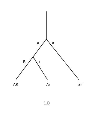
Figure 1: Two dichotomic phylogenetic trees involving a locus ${\mathcal{R}}$ in the genomic region of interest with the alleles $R$ (variant allele) and $r$ (wild type allele) and one marker loci ${\mathcal{A}}$ with alleles $A$ and $a$. The haplotypes formed at each ending branch are displayed at the bottom of the tree.

A marker-allele $A$ carries information about the locus ${\mathcal{R}}$ when the knowledge of the occurrence of $A$ determines the allelic form of ${\mathcal{R}}$. If the allele $A$ can occur together with the allele $R$ and the allele $r$, then $A$ is said to be neutral with respect to the locus ${\mathcal{R}}$. For instance, if the branching that formed the locus ${\mathcal{R}}$ occurred before the branching of the locus ${\mathcal{A}}$ and the branching of ${\mathcal{A}}$ occurred in the branch of the tree containing the allele $R$ (see Figure 1A), then the occurrence of the allele $A$ in the locus ${\mathcal{A}}$ implies that the locus ${\mathcal{R}}$ carries the allele $R$. Moreover, in that circumstances the occurrence of the allele $a$ does not imply neither that ${\mathcal{R}}$ carries the allele $R$ nor $r$. Therefore the allele $A$ carries information on the locus ${\mathcal{R}}$ and the allele $a$ is neutral with respect to ${\mathcal{R}}$.

Figure 2A illustrates a scenario where the branching of the locus ${\mathcal{R}}$ occurred first, which was followed by the branching of the locus ${\mathcal{A}}$ and then the branching of the locus ${\mathcal{B}}$. Moreover, the branching of the locus ${\mathcal{A}}$ occurred in the branch of the tree containing the allele $R$ while the branching of the locus ${\mathcal{B}}$ occurred in the branch of the tree containing the marker-allele $a$. Under these circumstances there are only four possible haplotypes: $AbR$, $aBR$, $abR$, $abr$. The allele $A$ only occurs together with the allele $R$, and it carries information about the locus ${\mathcal{R}}$. Analogously, the allele $B$ carries also information on the locus ${\mathcal{R}}$. Since the alleles $a$ and $b$ might occur together with both the allele $R$ and the allele $r$, then both $a$ and $b$ are neutral with respect to the locus ${\mathcal{R}}$. We can still draw further conclusions about the distribution of the information on the locus ${\mathcal{R}}$. If we want to use a rule for detecting the presence of the allele $R$ based on of the occurrence of marker-alleles, then the rule ’$R$ occurs when $A$ or $B$ occurs’ would detect two out of the three occurrences of the allele $R$. A rule based only on the occurrence of the marker-allele $A$ would only detect one out of the three possible occurrences of the allele $R$ and therefore would be less efficient in detecting $R$ than the rule using the alleles $A$ and $B$ together. The alleles $a$ and $b$ are both neutral and therefore the occurrence of the allele $R$ in the haplotype $abR$ cannot be detected using the information contained in the marker-alleles. We conclude that under the scenario described by Figure 2A, one can only detect the occurrence of the allele $R$ using a rule based on the marker-alleles in two out of the three possible haplotypes containing $R$. This maximum possible information recovery is attained only by the rule ’$R$ occurs when $A$ or $B$ occurs’.

A different scenario is described in Figure 2B where the branching in the locus ${\mathcal{A}}$ occurred first, followed by the branching in the locus ${\mathcal{R}}$, in the branch containing the allele $A$, and then the branching in the locus ${\mathcal{B}}$ in the branch of ${\mathcal{R}}$ containing the allele $R$. In this case the four possible haplotypes are: $ABR$, $AbR$, $Abr$ and $abr$. Therefore the marker-allele $B$ carries information on ${\mathcal{R}}$ and the marker-allele $A$ is neutral. The alleles $a$ and $b$ necessarily occur together and both carry information on ${\mathcal{R}}$ (but the same information). Here there are two cases in which the genotype of the locus ${\mathcal{R}}$ is determined by the genotypes of the marker-alleles: ’occurrence of $B$’ and ’occurrence of $a$ and $b$’ implying the occurrence of $R$ or $r$ respectively. Note that the last event ’occurrence of $a$ and $b$’ is equivalent to the event ’not occurrence of $A$ or $B$’. Under this scenario there are only two rules based on the marker-alleles genotypes that determine the genotype at the locus ${\mathcal{R}}$, both can be expressed as the effect of a combination of the occurrence of the marker-alleles $A$ and $B$. The first rule (’occurrence of $B$ implies occurrence of $R$’) can also be expressed as the effect of a single allele-marker as in the traditional inference method, but the second rule (’not occurrence of $A$ or $B$ implies the occurrence of $r$’) requires the use of groups of marker-alleles as in the models described in (3) to be properly represented in a statistical model. Here sticking only to rules based on single markers would represent a loss of half of the possibilities for determining the allele at the locus ${\mathcal{R}}$, that is a loss of half of the information on the genotype of the locus ${\mathcal{R}}$ that could be recovered with the knowledge of the marker-alleles.

Figure 3 displays the branching tree of a more complex scenario composed with the locus ${\mathcal{R}}$ in the genomic region of interest and four marker-loci ${\mathcal{A}}$, ${\mathcal{B}}$, ${\mathcal{C}}$, and ${\mathcal{D}}$, with alleles $A$, $a$, $B$, $b$, $C$, $c$, $D$ and $d$ respectively (we apply the same notational convention as before). The following six haplotypes are formed: $AbcdR$, $aBCdR$, $aBcdR$, $abcDR$, $abcdR$ and $abcdr$. Therefore, the rule ’if $A$ or $B$ or $C$ or $D$ occur then $R$ occurs’ detects four out of the five haplotypes containing the allele $R$. Moreover, under the current scenario, this is the best possible rule that could be constructed with the information on the marker-alleles that we have at hand. Although the allele $C$ carries information on the locus ${\mathcal{R}}$, this information is redundant since $C$ occurs always together with $B$. We can then remove the occurrence of the allele $C$ from the rule and still detect the same cases where the allele $R$ occurs when using the rule including the marker-alleles of the four marker loci.

The discussion above shows that in several situations the use of a naive representation of the effects of the marker-alleles is inefficient and that fully efficiency is obtained when using the approach involving the representation of groups of allele-markers. This phenomenon is not restricted to the few scenarios presented here. We claim, without giving a formal proof, that every time that there is a branching after the branching that generated the allele in the locus ${\mathcal{R}}$ the new marker-allele formed will carry information on the locus ${\mathcal{R}}$. Moreover, if the branching occurs in the branch that contains the wild type allele of the last branching of a marker locus, then the new marker allele formed will add new information on the locus ${\mathcal{R}}$ that is not contained in the marker-alleles formed before. This progressive gain of information obtained while the new marker-alleles are being formed is only fully realized if we use a rule of the type ’if $A$ or $B$ or $C$ or … occurs, then $R$ occurs’.

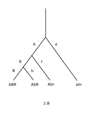
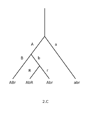
Figure 2: Three dichotomic phylogenetic trees involving a locus ${\mathcal{R}}$ in the genomic region of interest with the alleles $R$ (variant allele) and $r$ (wild type allele) and two marker loci ${\mathcal{A}}$ and ${\mathcal{B}}$ with alleles $A$, $a$, $B$, $b$ respectively. The haplotypes formed at each ending branch are displayed at the bottom of the tree.

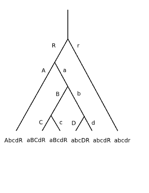
Figure 3: A complex dichotomic phylogenetic tree, involving a locus ${\mathcal{R}}$ in the genomic region of interest with the alleles $R$ (variant allele) and $r$ (wild type allele) and four marker loci ${\mathcal{A}}$, ${\mathcal{B}}$, ${\mathcal{C}}$ and ${\mathcal{D}}$. The haplotypes formed at each ending branch are displayed at the bottom of the tree.

3 Inference with a moderate number of
marker-alleles

3.1 Exhaustive search strategy

The strategy we propose for characterizing the association between a genomic region and a trait consists in searching exhaustively all the possible groupings formed with sets of marker-alleles and then choose the best candidate among the many possibilities. Here the best candidate is one that represents all the haplotypes of the genomic region of interest that are associated with the trait and that is not redundant. We define a grouping of the marker-alleles as a collection of non-empty disjoint subsets of the set of all marker-alleles. The subsets of a grouping are called marker-alleles groups (MAG). The idea is to use MAGs to represent haplotypes in the genomic region of interest that might be associated with the trait. For each possible grouping of the marker-alleles one statistical model of the type described by (3) containing factors representing each MAG of this grouping is fit. The grouping that generates the model with the best fit, according to a criterion to be defined below, is chosen to represent the association between the genomic region of interest and the trait. The grouping will be chosen in such a way that it will not contain redundancy, so each MAG will represent one haplotype in the region of interest. The number of MAGs in this grouping will be the number of detectable haplotypes associated with the trait. The magnitude of the effect of each MAG will be then the component of the magnitude of the haplotype that is detectable through the marker-alleles (which is smaller or equal to the magnitude of the effect of the unknown haplotype). This procedure is only feasible if the number of marker-alleles is not very large (we were able to analyse a data with 9 allele markers in few minutes in an ordinary personal computer).

It is convenient to make the exhaustive enumeration of all possible groupings of the marker-alleles in the following way. Consider the class ${\mathcal{P}}$ of all subsets of the set of marker-alleles $G=\{m_{1},\dots,m_{h}\}$. Formally, ${\mathcal{P}}$ is the class of parts of $G$. We associate one statistical model to each element $c$ of ${\mathcal{P}}$ by defining the model of the type defined by (3) that incorporate factors representing the groups of marker-alleles present in $c$. For $j=1,\dots,h$ let ${\mathcal{P}}_{j}$ be the class of all the subsets of $G$ containing exactly $j$ disjoint non-empty sub-sets. Clearly ${\mathcal{P}}$ is the disjoint union

$${\mathcal{P}}={\mathcal{P}}_{1}\cup\dots\cup{\mathcal{P}}_{h}\,.$$ (4)

Therefore we can search for the best models by proceeding in two steps: First we find the best model for each ${\mathcal{P}}_{j}$ ($j=1,\dots,h$) and then we find the best model among the candidates found in the first step. The selection of the best model related to a given ${\mathcal{P}}_{j}$ ($j=1,\dots,h$) is done by choosing the model with the largest value of the likelihood (or equivalently the log-likelihood) function. In this way the set of values of the likelihoods of the chosen candidate for each ${\mathcal{P}}_{j}$ is a profile set and plays a rule analogous to the rule of a profile likelihood curve for the number of marker-alleles. Denote the model that attains the maximum of the likelihood for a given ${\mathcal{P}}_{j}$ by $M_{j}$ and the value log-likelihood function of $M_{j}$ at the maximum by $\hat{l}_{j}$ (for $j=1,\dots,h$). We refer to these quantities as the profile model and the profile log-likelihood of order $j$.

3.2 Determination of the number of detectable associated haplotypes

The next step in the procedure of inference is to choose the class ${\mathcal{P}}_{j}$ ($j=1,\dots,h$) that yields the best statistical model. If we assume that the haplotypes in the genomic region of interest are representable in terms of subsets of $G$, then choosing the class ${\mathcal{P}}_{j}$ that produces the best statistical model is equivalent to infer the number of detectable haplotypes in the genomic region of interest.

The profile log-likelihood never decreases when the number of haplotypes assumed in the model increase, i.e.

$$\hat{l}_{1}\leq\dots\leq\hat{l}_{h}\,\,,$$ (5)

since a model $M_{i}$ ($i<h$) can be expressed as a sub-model of a model with $i+1$ MAGs in which a pair of MAGs present the same effect. As a consequence, it is not reasonable to estimate the number of haplotypes in the region of interest by choosing the ${\mathcal{P}}_{j}$ with larger log-likelihood. We argue next that maximizing the negative Akaike information (or a variant of it) is a reasonable procedure for inferring the number of haplotypes in the genomic region of interest.

The inequality (5) does not extract all the information available on the development of the profile likelihood curve as the number of putative haplotypes of the genomic region of interest increases. Indeed, the profile log-likelihood curve is expected to increase significantly with the number of putative haplotypes until the number of detectable haplotypes is reached. After that point the profile log-likelihood curve is supposed to remain approximately constant. To see that, consider the situation where there are $J$ associated haplotypes in the genomic region. If $j<J$, then the model $M_{j}$ fails to represent at least one haplotype and then the profile log-likelihood should increase in a statistically significant way with the addition of the possibility to represent one more haplotype. Once attained the number of haplotypes the gain obtained by increasing the capacity of the model to represent one more haplotype vanishes and only marginal gains in the profile log-likelihood are expected (see figure 4). We assume implicitly here that there are no significant mixtures in the data and that the model is not missing any important explanatory variable (see Figure 4) The informal argument above suggests we can infer the number of detectable haplotypes in the genomic region by searching for the point at which the profile log-likelihood curve remains (approximately) constant. One way to do that is to subtract a suitable quantity from the profile log-likelihood. By doing that, the new adjusted profile log-likelihood would decrease approximately linearly in the region where the original profile log-likelihood was constant (i.e. when the assumed number of haplotypes is larger than the number of detectable haplotypes in the genomic region of interest). If the subtracted quantity is not too large, the adjusted profile log-likelihood curve will still increase in the region where the original profile log-likelihood is increasing significantly (before attaining the number of detectable haplotypes). The so called Akaike information criterion (Akaike, 1974, Burnham and Anderson, 2002) explores this idea and is equivalent to subtract the number of parameters in the model from the log-likelihood. In fact the Akaike information $AIC$ is defined as minus twice the difference of the log-likelihood and the number of parameters, more precisely,

$$AIC=-2\left\{\log({\hat{L}})-k\right\}\,\,,$$

where $k$ is the number of parameters in the statistical model, and ${\hat{L}}$ is the maximized value of the likelihood function for the estimated model. Minimizing the Akaike information is equivalent to maximizing the log-likelihood adjusted by subtracting the number of parameters in the model. This apparently arbitrary choice for the quantity subtracted from the log-likelihood can be justified as being equivalent to subtract from a likelihood ratio statistic its (asymptotic) expected value. Alternatively, one might subtract $3.85k$ from the profile log-likelihood which would be equivalent to perform a likelihood ratio test for incorporating the representation of an additional haplotype to the current model when working at a significance level of 5%.

Summing up, the procedure we propose is to maximize the log-likelihood in each class ${\mathcal{P}}_{i}$ (which is equivalent to minimize the AIC in this class of models since all the models in ${\mathcal{P}}_{i}$ has by construction the same number of parameters), for $i=1,\dots,h$, and then choose the model with the smaller (profile) AIC (or equivalently, with the larger adjusted profile log-likelihood).

4 Example: Chicken susceptibility to
helminths

The association between the susceptibility to the helminth Ascaridia galli in chickens and the major histocompatibility (gene) complex (MHC) was investigated in two recent studies (Schou et al, 2007, 2008). These studies used the microsatellite LEI0258 (Fulton et al., 2006), which is located in a non-coding region between two contiguous regions of the MHC gene complex (the B-F/B-L and the BG loci), to obtain eight polymorphic marker-alleles here denoted 195bp, 207bp, 219bp, 251bp, 264bp, 276bp, 297bp and 324bp. Since recombination within the chicken MHC is very rare (Plachy et al., 1992; Miller et al., 2004), the alleles of the microsatellite LEI0258 are expected to be in tight linkage disequilibrium with haplotypes formed by alleles at the BF/BL and the BG loci (i.e. the MHC haplotypes). Moreover, we can discard the possibility of a direct effect of the LEI0258 alleles since this marker is located in a non-coding region (as any microsatellite marker). Therefore it is reasonable to apply the techniques described above using the alleles of the microsatellite LEI0258 as marker-alleles in the set-up described above.

In the first study (Schou et al, 2007) the intensity of infection with A. galli was determined for birds of two chicken breeds by counting the number of this worms found in the intestine of each of the birds examined. The counts were categorized as, zero, low (up to 3 counts), intermediate (4 to 10 counts) and high (more than 10 counts). The cut-off points used for defining the categories above were chosen in such a way that the losses of the Külback-Leiber information about the counts due to a discretization were minimized. The association between the intensity of infection and the MHC haplotypes was studied by applying a baseline-category logits model for multinomial distributed data (Agresti, 1990) using the zero-category as a reference. Inference in these models can be performed by fitting three logistic models constructed with a common reference category (Agresti, 1990) which can be done by using standard generalized linear models (with a binomial distribution and a logistic link). The standard method was used in this study and an association was declared if the effect of a marker-allele, in the presence of the other marker-alleles, was statistically significant. Using this procedure it was found that the occurrence of the marker-allele 276bp was associated with an increased resistance. No further associations were found with the standard procedure.

A second study (Schou et al, 2008) was independently performed with different birds of the same two chicken breeds. In this study the birds were inoculated with A. galli under controlled experimental conditions and the fecal excretion of A. galli eggs was monitored. Each animal was classified based on the counts of eggs as presenting zero, low, intermediate or high infection level. A baseline-category logits model was applied but, differently from the first study, using the strategy of searching for marker-allele groups (MAG). Three marker-allele groups, denoted MAG-1, MAG-2 and MAG-3, were identified and found to be associated with the intensity of infection with A. galli. Figure 4 displays the profile log-likelihood and profile Akaike information as a function of the number of MAGs assumed to be associated to the infection level. A joint likelihood ratio test indicated a statistically significant effect of these three MAGs on the intensity of infection (p=0.0013). MAG-1 was formed by the LEI0258 alleles 297bp and 324bp; MAG-2 was composed of the alleles 195bp, 207bp, 219bp and 264bp; and MAG-3 only contained the allele 276bp. Detailed analyses revealed that animals carrying MAG-1 or MAG-3 presented larger resistance to A. galli, while MAG-2 was associated with augmented susceptibility (Schou et al, 2008).

An a posteriori analysis of the data of the first study using the strategy of searching for marker-allele groups yielded the same significant marker-allele groups with MAG-1 and MAG-3 associated to resistance and MAG-2 associated to susceptibility to A. galli (reported in Schou et al, 2008). Note that when applying the standard strategy only the effect of the marker-allele 276bp was found significant, which is equivalent of detecting the marker-allele group MAG-3 (composed only by the allele 276bp). None of the marker-alleles composing the marker-allele group MAG-1 and MAG-2 (i.e. 297bp, 324bp, 195bp, 207bp, 219bp and 264bp) presented an individual significant effect, which illustrates the loss of power to detect association when applying the standard modelling strategy.

Figure 4: Profile log-likelihood, negative profile Akaike information (dashed and dotted line) and negative profile alternative Akaike information (dotted line) as a function of the assumed number of marker-allele groups for the data of the second study on susceptibility to A. galli (Schou et al, 2008). The dashed horizontal line represents the log-likelihood of a model containing the maximum number of marker-allele groups (i.e. 8) evaluated at its maximum, that is, an upper bound for the values of the profile log-likelihood. The alternative Akaike information was obtained by subtracting $3.85k$ for each successive increase in the number of marker-allele groups, corresponding to test the incorporation of one more marker-allele group at a 5% level of significance. The value 10 was added all the values of the negative alternative profile Akaike information for graphical convenience. The negative profile Akaike information and the alternative negative profile Akaike information presented both a maximum at 3 suggesting the presence of 3 detectable marker-allele groups.

5 Discussion

We presented a strategy for performing statistical inference that allows to represent the occurrence of non-observable alleles or haplotypes in a genomic region of interest in terms of a range of observable marker-alleles at highly linked loci. The kernel idea presented here is that the natural unit to build statistical models under this context are not the marker-alleles but groups of marker-alleles. As argued due to the way haplotypes in a genomic region of relatively small size (such that allow us to ignore recombination) are formed during the evolution of a population, certain haplotypes formed with marker-alleles will occur naturally in tight linkage disequilibrium with (non-observable) haplotypes in the genomic region. The way these marker-allele haplotypes are constituted imply that detection rules based on indication functions of groups of marker-alleles are optimal in the sense that they allow to extract the maximum possible amount of information that is contained in the marker-alleles. Naive representations constructed exclusively with groups of allele-markers with only one element are bounded to use inefficiently the information (if not destroy it completely), as illustrated in an example with real data.

The techniques presented here involve fitting many models and selecting a best candidate among the (very) many possibilities, following a sequence of models with increasing number of assumed marker-allele groups. This order is tough to facilitate the inference of the number of marker-allele groups with detectable effect on the trait of interest. However, this force brut exhaustive search is not feasible for a large number of marker-alleles, since the number of possibilities to be checked increases very rapidly with the number of marker-alleles. An alternative is to use Monte Carlo based algorithms for maximization in discrete parameter space as simulated annealing or the genetic algorithm.

We showed that the classical criterion of maximizing the log-likelihood cannot be used to estimate the number of detectable marker-alleles groups, since the likelihood function cannot decrease with the number of MAGs. A way around that is to use the Akaike information criterion which penalizes the log-likelihood of models with too many (unnecessary) parameters. Other forms of penalized likelihood could be applied, as for instance the alternative information criterion proposed in the text, which is equivalent to perform a likelihood ratio test for incorporating one extra MAG in the model (at a 5% level of significance). The choice of the penalized likelihood method to be used depend on the type of basic statistical model used.

We used generalized linear models to explain our ideas, but we stress that other models could had been used without essentially changing the procedure exposed here. Indeed, the example presented uses in fact a slight extension of generalized linear models. Probably one of the most relevant extensions would be the incorporation of random components allowing to represent population structure, co-ancestry and polygenic effects. Another possibility to be explored is the incorporation of information on ancestors genotypes and other mechanisms of inheritance. In conclusion, the techniques presented here are flexible and relatively easy to implement using classical statistical models and standard software.

Acknowledgements:
This work originated during the statistical analysis of the data collected by Torben Wilde Schou. We thank him for kindly allowing us to present part of his data as an example.

References

- [1] Akaike, H., (1974). New Look at Statistical-Model Identification. IEEE Transactions on Automatic Control 19 (6), 716-723.
- [2] Burnham, K. P., and Anderson, D.R. (2002). Model Selection and Multimodel Inference: A Practical-Theoretic Approach, 2nd ed. Springer-Verlag. ISBN 0-387-95364-7.
- [3] Fulton, J.E., Juul-Madsen, H.R., Ashwell, C.M., McCarron, A.M., Arthur, J.A., O’Sullivan, N.P. and Taylor, R.L., Jr.(2006). Molecular genotype identification of the Gallus gallus major histocompatibility complex. Immunogenetics 58 (5-6), 407-421.
- [4] Jørgensen, B., Labouriau, R. and Lundbye-Christensen, S. (1996). Linear growth curve analysis based on exponential dispersion models. J.R. Statist. Soc. B 58, No. 3, 573-592.
- [5] Miller, M.M., Bacon, L.D., Hala, K., Hunt, H.D., Ewald, S.J., Kaufman, J., Zoorob, R. and Briles, W.E.(2004) Nomenclature for the chicken major histocompatibility (B and Y) complex. Immunogenetics 56 (4), 261-279.
-
[6]
Orru S., E. Giuressi, M. Casula, A. Loizedda, R. Murru, M. Mulargia,
M.V. Masala, D. Cerimele, M. Zucca, N. Aste, P. Biggio, C. Carcassi, L.
Contu (2002).
Psoriasis is associated with a SNP haplotype of the corneodesmosin gene (CDSN).
Tissue Antigens 60 (4), 292-298.
doi:10.1034/j.1399-0039.2002.600403.x - [7] Plachy, J., Pink, J.R.L. and Hala, K. (1992). Biology of the Chicken Mhc (B-Complex). Crit. Rev. Immunol. 12 (1-2), 47-79.
- [8] Schou, T.L.H, Permin, A., Juul-Madsen H.R., Sørensen P., Labouriau R., Nguye T.L.H, Fink M. and Pham S.L. (2007). Gastrointestinal helminths in indigenous and exotic chickens in Vietnam : association of the intensity of infection with the Major Histocompatibility Complex. Parasitology, 134, 561-573.
- [9] Schou, T.L.H, Labouriau, R., Permin, A., Christensen, J.P., Sørensen, P., Cu, H.P., Nguyen, K. N. and Juul-Madsen, H.R. (2008). MHC haplotype and susceptibility to experimental infections (Salmonella Enteritidis, Pasteurella multocida or Ascaridia galli) in a commercial and an indigenous chicken breed. Paper III in the PhD thesis “Genetic diversity of poultry in extensive production systems and its implications for disease resistance” by Torben Wilde Schou, Department of Veterinary Pathobiology, Faculty of Life Sciences, University of Copenhagen, Denmark (submitted).