Structural Ordering and Antisite Defect Formation in Double Perovskites

Abstract

We formulate an effective model for B-B’ site ordering in double perovskite materials A₂BB’O₆. Even within the simple framework of lattice-gas type models, we are able to address several experimentally observed issues including nonmonotonic dependence of the degree of order on annealing temperature, and the rapid decrease of order upon overdoping with either B or B’ species. We also study ordering in the ‘ternary’ compounds A₂BB’_1-yB”_yO₆. Although our emphasis is on the double perovskites, our results are easily generalizable to a wide variety of binary and ternary alloys.

I Introduction

Double perovskite (DP) materials of the form A₂BB’O₆ are being actively studied dp-rev on account of their unusual electronic and magnetic properties. In particular, some double perovskites, e.g, Sr₂FeMoO₆, show half-metallic behaviour, high ferromagnetic $T_{c}$, and large low field magnetoresistance. Remarkably, there are also double perovskites that are antiferromagnetic and insulating. The metallic and magnetic character depends primarily on the choice of B and B’, but is also affected by the local ordering of these ions.

While it is desirable to understand the interplay of structural, electronic and magnetic variables in these materials within an unified framework, it is technically daunting to ‘anneal’ all these degrees of freedom simultaneously. We argue that it is reasonable to abstract the problem of structural order, solve it, and then set up the electronic-magnetic problem on the appropriate structural motif. Our paper is organised as follows. In the next section we present the overall model for the DP’s, involving the structural, magnetic and electronic degrees of freedom, and indicate how an effective structural model can be formally extracted. The section after, discusses a phenomenological model for structural order. We then discuss our method and computational variables. This is followed by the results, first on ‘ordering’ for materials of the form A₂BB’O₆, then for the ‘doped’ cases, A₂B_1+xB’_1-xO₆, and finally for the ternary systems, A₂BB’_1-yB”_yO₆. We conclude with a summary of our results.

II Structural order and magnetism

The magnetism in the DP’s is intimately related to electron delocalisation, which in turn depends on the spatial pattern of B, B’ ions KimCheong ; Martinez ; GarciaLanda . Let us write down the Hamiltonian in terms of the electronic and magnetic degrees of freedom to illustrate the crucial role of spatial B-B’ order. Let B be the ‘magnetic’ ion and B’ the non magnetic one. We define a binary variable $\eta_{i}$, such that $\eta_{i}=1$ when a site has a B ion, and $\eta_{i}=0$ when a site has a B’ ion. The $\eta$’s will encode the atomic positions. In terms of these, the model for the DP’s is:

$$H =\epsilon_{B}\sum_{i}\eta_{i}f_{i\sigma}^{\dagger}f_{i\sigma}+\epsilon_{B^{\prime}}\sum_{i}(1-\eta_{i})m_{i\sigma}^{\dagger}m_{i\sigma}$$ (4)

$$~{}-t\sum_{<ij>\sigma}\eta_{i}(1-\eta_{j})f_{i\sigma}^{\dagger}m_{j\sigma}$$

$$~{}+J\sum_{i}\eta_{i}{\bf S}_{i}\cdot f_{i\alpha}^{\dagger}\vec{\sigma}_{\alpha\beta}f_{i\beta}+J_{AF}\sum_{\langle ij\rangle}\eta_{i}\eta_{j}{\bf S}_{i}.{\bf S}_{j}$$

$$~{}+V_{at}\{\eta\}$$

The $f$ operators refer to the magnetic B sites and the $m$ to the non magnetic B’. $\epsilon_{B}$ and $\epsilon_{B^{\prime}}$ are level energies, respectively, at the B and B’ sites, $\Delta=\epsilon_{B}-\epsilon_{B^{\prime}}$ is the ‘charge transfer’ energy, and $t$ is the hopping amplitude between nearest neighbour B and B’ ions. We have ignored orbital degeneracy in the present model. ${\bf S}_{i}$ are the moments on the B site, $J$ is the Hunds coupling on those sites, and $J_{AF}$ is the antiferromagnetic (AF) superexchange coupling between B moments when two B ions neighbour each other. The $V_{at}\{\eta\}$ represent atomic interactions between the B, B’ ions.

In the simplest case of equal proportions of B and B’ ions, and their perfect alternating arrangement, each B is coordinated by B’ only and vice versa. The AF coupling does not come into play, and electron delocalisation on the B-B’ network generally prefers a ferromagnetic spin configuration. This state is also highly conducting. However, if the atomic order is imperfect and there are B ions neighbouring each other, two B moments get locked into an antiparallel configuration. This leads to a reduction in the overall ferromagnetic moment, and these ‘antisite’ regions also hinder electron transport. The magnetism and transport is obviously strongly dependent on the structural motif. What decides the atomic B-B’ arrangement? Let us look at the formal answer first.

For large $S$ spins, the DP model refers to electrons coupled to classical magnetic moments and moving in a background defined by $\{\eta\}$. If the atomic ordering problem is to be isolated from this, one should ‘trace out’ the electronic and magnetic variables. The effective potential $V_{eff}\{\eta\}$ controlling atomic order is

$$V_{eff}\{\eta\}=-(1/\beta)log\int{\cal D}{\bf S}_{i}Tr_{\{f,m\}}e^{-\beta H}$$

Computing $V_{eff}$ and ‘updating’ atomic positions accordingly is a computationally demanding task, the Monte Carlo (MC) equivalent of a Car-Parinello simulation. There is limited information about $V_{at}$, and the ‘trace’ is technically difficult, so we construct a simple $V_{eff}\{\eta\}$ that is consistent with the phenomenology, rather than attempt an elaborate ‘first principles’ calculation. We motivate this in the next section.

III Model for atomic ordering

The ideal DP with the general formula A₂BB’O₆ has ordering of B and B’ atoms at the center of alternate O₆ octahedra. Focusing only on the B and B’ ions, the ideal structure is simply an alternation of B and B’ ions along the ${\hat{x}}$, ${\hat{y}}$ and ${\hat{z}}$ axis. However, in imperfectly annealed systems, there can occur antisite defect regions where this ordering is reversed, and two B atoms or two B’ atoms occur adjacent to each other. The ordering of the B-B’ is in general neither ‘perfect’ nor random, it is the result of an annealing process. While samples with high degree of order have been grown Kobayashi , indicating that the atomic order in the structural ground state should be perfect, recent experiments reveal an interesting trend in the degree of order as a function of annealing temperature.

In the experiments by Sarma et. al. ord-expt-prl on Sr₂FeMoO₆ it was observed that there was a non-monotonic dependence of the degree of Fe-Mo ordering upon the annealing temperature, $T_{ann}$, as shown in Fig.1. The different samples were taken from the same ‘parent’ material (synthesised at high temperature and quenched to a low temperature), heated to a temperature $T_{ann}$, and annealed there for a duration $\tau_{ann}$, say.

If there is indeed a B-B’ ordering tendency in the DP’s, the extent of order at equilibrium would be highest at low $T_{ann}$, progressively falling off at higher $T_{ann}$ where the order is expected to be small. The downturn at low annealing temperature, it seems reasonable, is due to insufficient equilibriation. Our model below and results are based on the assumption that: (i) there is an intrinsic B-B’ ordering tendency in the DP’s, (ii) given long equilibriation time, the DP’s would indeed show a high degree of order at low $T$, but (iii) under typical synthesis conditions/annealing protocol the system only manages to generate correlated configurations with short range order. The annealing temperature and annealing time are therefore key to quantifying the structural order.

Since the structural (dis)order seems to be ‘frozen’ at temperature, $T\sim 1000$K, much above the temperature for magnetic order ($\sim 400$K), the qualitative issues in atomic ordering can be understood by ignoring the electronic-magnetic variables in an effective model, below.

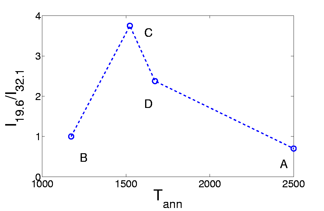
Figure 1: Experimental data for ordering vs annealing temperature, obtained by Sarma et. al

In the absence of detailed microscopic knowledge about $V_{eff}\{\eta\}$, we used a binary lattice gas model that has the same ordering tendency as the real materials, viz, B-B’ alternation, or equivalently a ‘checkerboard’ pattern. In terms of the variables $\eta_{i}$, the simplest such model is:

$$V_{eff}\{\eta\}=V\sum_{\langle ij\rangle}\eta_{i}(1-\eta_{j})$$ (5)

with $V>0$ being a measure of the ordering tendency. The ground state in this model would correspond to $\eta=1,0,1,0,..$ along each axis, i.e, B, B’, B, B’.. Notice that this approach tries to incorporate the effect of complex interactions between the A, B, B’ and O ions (as also the electrons) into a single parameter (See Appendix).

This binary model is equivalent to a nearest neighbour Ising model, so the equilibrium physics is very well understood staufferbook . We, however, want to explore the consequences of different annealing protocols on this model, to examine the consequences of imperfect annealing. The qualitative ordering effects in the lattice gas model are similar in 2D and 3D, so we work with a 2D structure since it allows ease of visualisation.

IV Method

The atomic order that emerges from $V_{eff}$ can be studied with mean field theory if the system is in equilibrium. However, we want to explore non equilibrium effects due to poor annealing, so we use a Monte Carlo technique to anneal the $\eta$ variables. Most of our studies involve a protocol where we start with a completely random B-B’ configuration (as if quenched from very high $T$), and then anneal it at a temperature $T_{ann}$, for a MC run of duration $\tau_{ann}$ Monte Carlo steps (MCS). Since the number of B and B’ atoms is fixed we update our configurations by (i) moving to some site ${\bf R}_{i}$, (ii) attempting an exchange of the atom at ${\bf R}_{i}$, with another randomly picked within a box of size $L_{C}^{2}$ centred on ${\bf R}_{i}$, and (iii) accepting or rejecting the move based on the Metropolis algorithm. We have used system size $L=20,~{}40,$ and $80$, update cluster with $L_{C}=4,$ and $10$, $T_{ann}/V$ ranging from $0.01-0.3$, and $\tau_{ann}\sim 200-30000$ MCS. We have studied the structure factor, and also detailed spatial configurations, to quantify the extent of order.

V Ordering with equal proportions of B, B’

This section discusses the order in systems where the number of B and B’ ions is equal, and perfect order is in principle possible. In an attempt to mimic the experimental annealing protocol, we started with random initial configurations at some temperature $T_{ann}$ and annealed for some time $\tau_{ann}$. The structure factor $S({\bf q})$ at the ordering wavevector, $\{\pi,\pi\}$, is averaged over 40 such initial configurations. The extent of order, quantified by the peak in $S({\bf q})$, is shown in Fig.2(a) for a lattice size $20\times 20$, and in Fig.2(b), for a lattice size $40\times 40$.

There are two noteworthy features in the data in Fig.2. (i) The non monotonic behaviour with $T_{ann}$ that we anticipated indeed shows up in the structure factor peak, and (ii) there is a strong size dependence of the peak in $S(\pi,\pi)$, varying almost by a factor of 4 between $L=20$ and $L=40$!

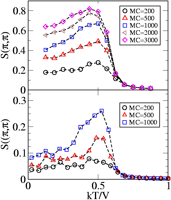
Figure 2: $\pi-\pi$ structure factor vs $T_{ann}$ on a $20\times 20$ lattice, for different Monte Carlo runlength (annealing time). $20\times 20$ lattice (top) and $40\times 40$ lattice (bottom).

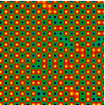
Figure 3: Non-equilibrium, $T_{ann}=0.5$ configuration for $\tau_{ann}=100$.

The downturn in $S(\pi,\pi)$ at low $T_{ann}$ is due to the inability of the system to achieve equilibrium, at short annealing time, when one starts with a random initial configuration. With increasing $\tau_{ann}$ there is of course an increase in the extent of order (for given $T_{ann}$ and $L$) and $S(\pi,\pi)$ reaches $\sim 0.6$ of the equilibrium value for $L=20$, for MCS=1000. At $L=40$, however, this is suppressed to $\sim 0.1$ of the equilibrium value, for the same MCS. This origin of this strong size dependence becomes apparent when we examine a typical configuration at low $T_{ann}$, generated by a short annealing run, $\tau_{ann}=100$ MCS, in Fig.3

The ordering is obviously imperfect, as $S(\pi,\pi)$ suggested, more interestingly, the system actually consists of a few large ordered clusters with ‘phase slip’ between them. While locally these domains are well ordered, the bulk $S(\pi,\pi)$ arises from the interfering contribution of large domains, and this ‘cancellation’ depends strongly on the system size $L$. In the smaller systems, $L\sim 20$, $S(\pi,\pi)$ is decided by the larger domain, and as domains proliferate with increasing $L$, there is an increasingly better cancellation between the out of phase domains, and $S(\pi,\pi)$ falls.

Since the antisite regions are at the interface of two ordered (but phase slipped) clusters, in what follows we show the domains and domain walls, rather than the detailed atomic configuration.

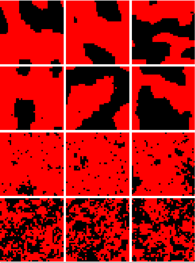
Figure 4: Domain pattern for different $T_{ann}$ and equilibriation time. Left column, $\tau_{MC}=1000$, center $\tau_{MC}=500$, right $\tau_{MC}=200$. Rows, top to bottom, $T=0.1,~{}1.0,~{}2.0,~{}3.0$. The antisite defects are at the domain boundary.

In Fig.4 one corner site in each panel is set as reference and the others ‘coloured’ in terms of their phase relation to it. For concreteness assume the atom at bottom left corner is B. Let this site be ${\bf R}_{0}=\{0,0\}$, and index all sites in terms of integers, $\{R_{ix},R_{iy}\}$. Then the ‘correct’ order would require that the atom at ${\bf R}_{i}$ be B if $R_{ix}+R_{iy}$ is even, and B’ if $R_{ix}+R_{iy}$ is odd. Formally, we just plot $f(\eta_{i})=\eta_{i}e^{i\pi(R_{ix}+R_{iy})}$, with a light colour for a site that is correctly ordered with respect to the origin, and dark if it is not.

The result of this, on a $40\times 40$ lattice, is shown in Fig.4. The columns correspond to different $\tau_{ann}=1000,~{}500,~{}200$ MCS, left to right, and the rows to $T_{ann}=0.1,~{}1.0,~{}2.0,~{}3.0$, top to bottom. At larger annealing and intermediate $T_{ann}$ we see a large single domain dominating the configuration, while at low or high $T_{ann}$ and short $\tau_{ann}$ the structure is more fragmented. In the electron problem, the domains themselves are likely to be ‘homogeneous’ ferromagnetic regions, while the antisite regions, with neighbouring B-B atoms might be antiferromagnetic.

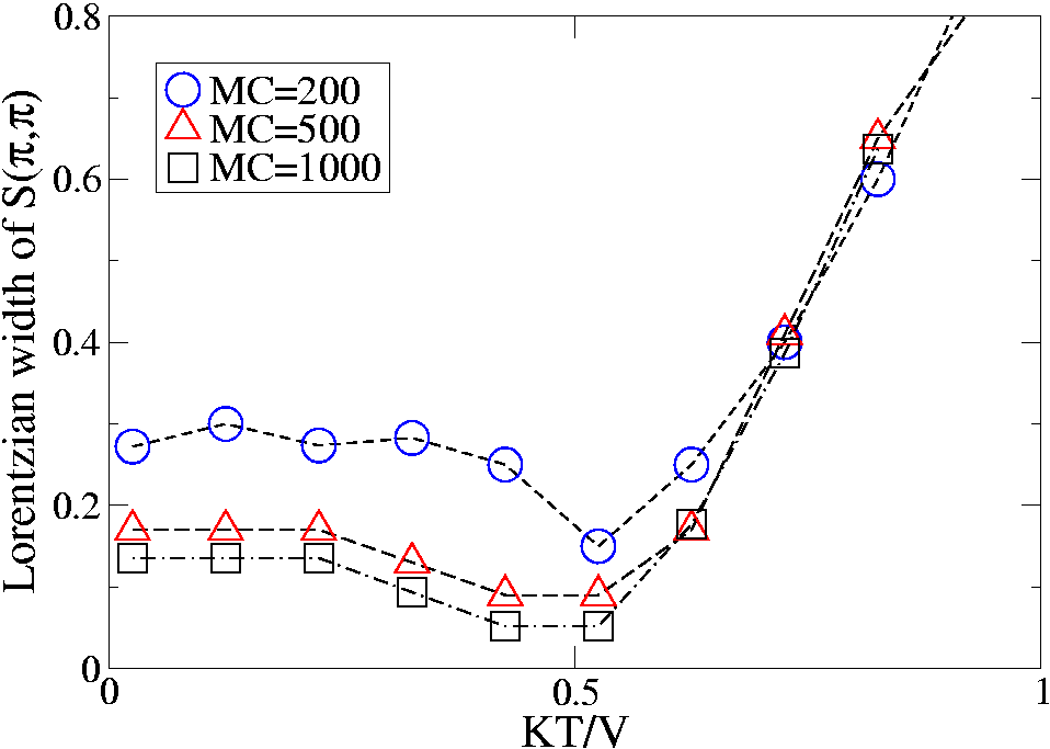
Figure 5: The Lorentzian width in the structure factor peak, to estimate the domain size/correlation length.

In an attempt to quantify the size of the clusters as a function of $T_{ann}$ and $\tau_{ann}$ we studied the full structure factor $S({\bf q})$, averaged over $\sim 50$ configurations, and fitted the ordering peak to a lorentzian of the form

$$S({\bf q}\sim\{\pi,\pi\})\approx A(\Gamma/\pi)/((q_{x}-\pi)^{2}+(q_{y}-\pi)^{2}+\Gamma^{2})$$

$A$ is an overall amplitude factor and $\Gamma(T_{ann},\tau_{ann})$ is a measure of the (inverse) width of the cluster size. This is shown in Fig.5.

We also tried a protocol where a system is heated to a temperature $T_{f}$ but gradually, through a sequence $T_{1},~{}T_{2},..$, retaining the memory of configurations at the earlier temperature. The result of this slow annealing is similar to the earlier protocol, i.e, non-monotonic for short $\tau_{ann}$, and tends towards the monotonic equilibrium response with increasing $\tau_{ann}$. For $\tau_{ann}>10^{4}$, we obtain essentially the equilibrium profile except at very low $T$. The results are in Fig.6.

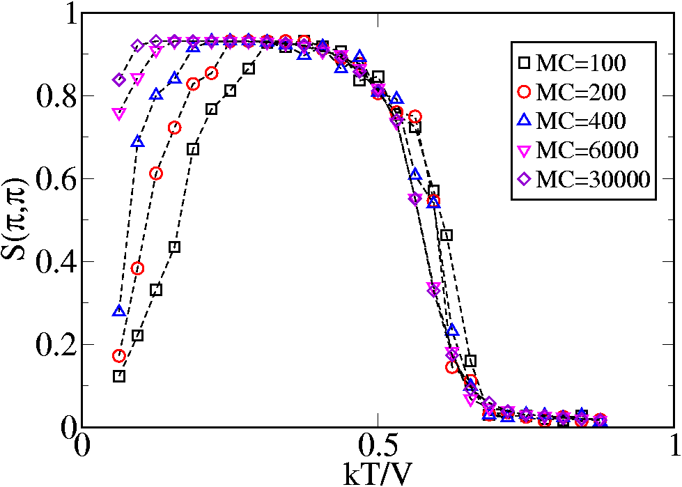
Figure 6: $\pi-\pi$ structure factor vs $T$ for heating run with memory for different Monte Carlo steps (annealing time)

VI Ordering with unequal proportions of B, B’

When the B-B’ proportion is not 1:1 it is obviously not possible for every B to be coordinated by B’ and vice-versa. ‘Antisite’ regions, rich in B or B’, would exist even at equilibrium. Our attempt, in this section is (i) to capture the loss of B-B’ order with increasing concentration of B’, say, and also (ii) to study the effect of restricted annealing on the system.

Our reference for (i) above are the results of D. Topwal, et. al. topwal , who had prepared the series of samples Sr₂Fe_1+xMo_1-xO₆, with proportion of Fe in excess of Mo. Such samples would have antisite defects even when the sample is well equilibriated. The XRD pattern for these set of samples is given in Fig.7. They observed that the peak at $19.6^{\circ}$, related to checkerboard ordering, decreases uniformly for both positive as well as negative $x$. In particular, the peak is observed to be almost absent in the $x=0.5$ sample.

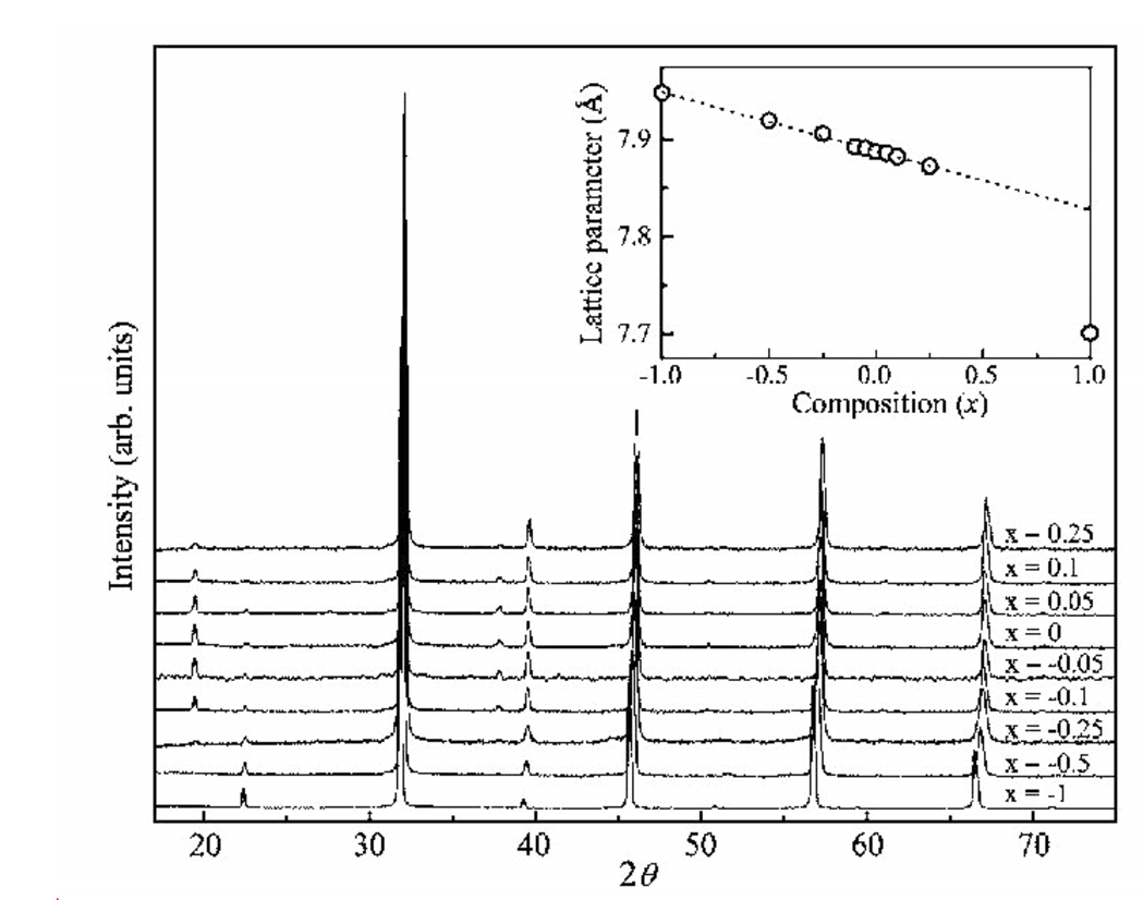
Figure 7: XRD data for different Fe-Mo proportions, obtained by Topwal et. al topwal

Before embarking on a MC study of this problem it is useful to establish the results of a simple mean field study of B-B’ order (at equilibrium) for varying $x$. Fig.8 shows the result of such a calculation, done via the mapping of the lattice gas to an Ising model at constant ‘magnetisation’ (which corresponds to the difference in concentration of B and B’). One can capture this effect within mean field theory by considering an AF Ising model at different magnetic fields, and computing the AF order parameter, i.e, the ordering peak, and the magnetisation. As seen in Fig.8, the $\{\pi,\pi\}$ ordering at low temperatures decreases uniformly with increasing magnetization. However, it truly vanishes only when the magnetization is unity, correponding to a purely B (eg. Fe) or B’ (eg. Mo) compound. This does not correspond to the experimental situation.

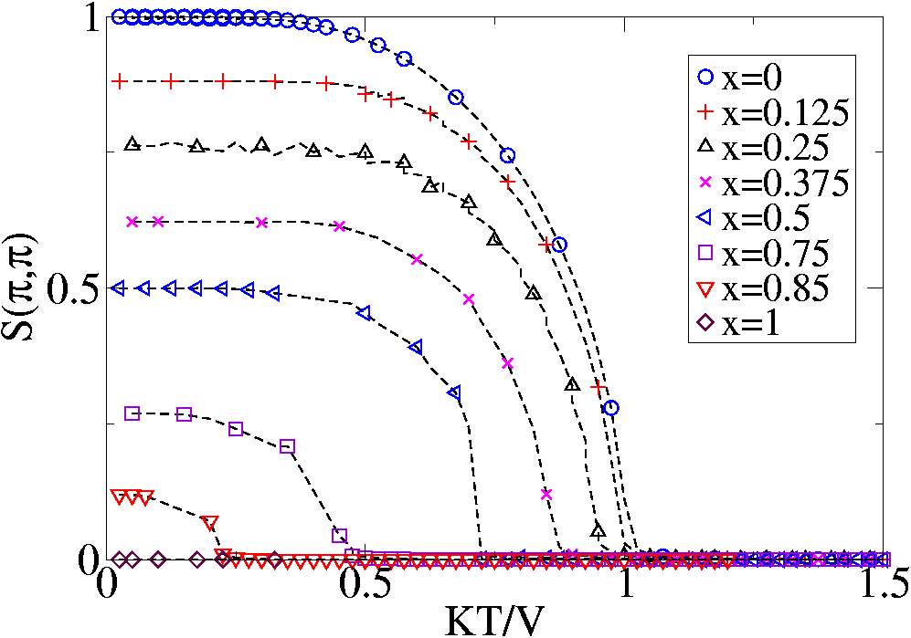
Figure 8: Structure factor at ($\pi,\pi$) from mean field theory for different B-B’ proportions

Next we did Monte Carlo simulations for the Ising model for different non-zero values of magnetization. The results for cooling runs are shown in Fig.9. The $\{\pi,\pi\}$ ordering is found to almost vanish at $x=0.5$, much before the mean field prediction. Interestingly, the experimental XRD data at $x=0.5$ does not seem to show the $19.6^{\circ}$ peak related to ordering either.

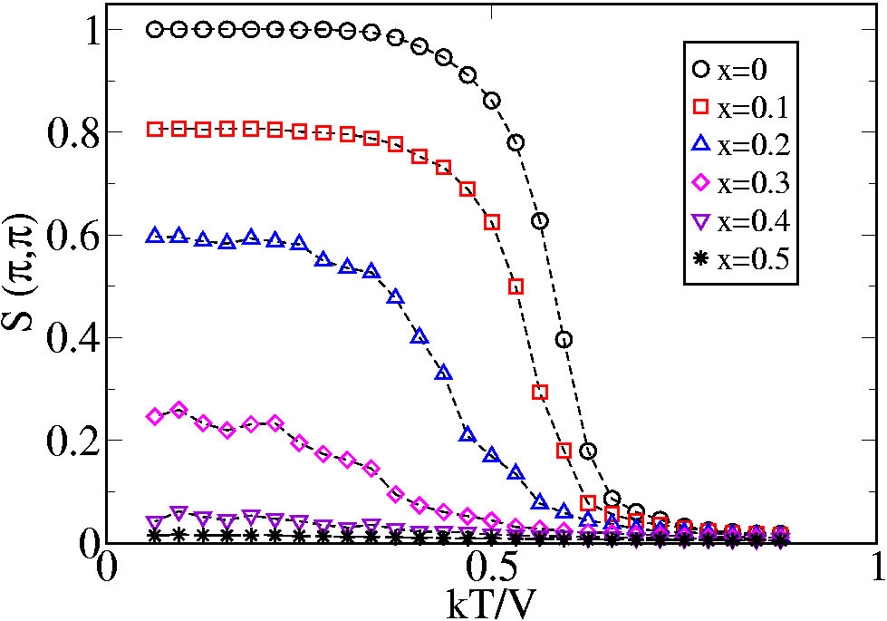
Figure 9: Structure factor vs T (cooling runs) for different B-B’ proportions.

For any specific proportion, $x=0.1$, say, the variation of $S(\pi,\pi)$ with $T_{ann}$ is shown in Fig.10, for various $\tau_{ann}$. The overall behaviour is similar to that for equal B-B’ proportions, namely that the non-monotonicity decreases upon increasing annealing time, and gradually approaches the equilibrium cooling curve. Since the equilibrium saturation value of the $(\pi,\pi)$ structure factor in this case is less than 1, hence the maximum values of the non-equlibrium curves for any given value of MC steps is less than the corresponding value for the equal proportion case.

In Fig.11, on the other hand, the annealing time is kept fixed, while the proportions are varied. While $S(\pi,\pi)$ obviously has a nonmonotonic dependence on $T_{ann}$, the maximum values progressively increase with decreasing $x$ as expected. In the case of annealing with memory, as shown in Fig.12, the behaviour is once again nonmonotonic, except that the maximum of the structure factor nearly always hits the equilibrium value.

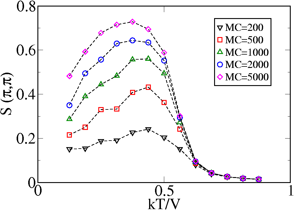
Figure 10: Structure factor vs T (heating run without memory) for $x=0.1$, different Monte Carlo steps/spin. Average over 300 initial configurations.

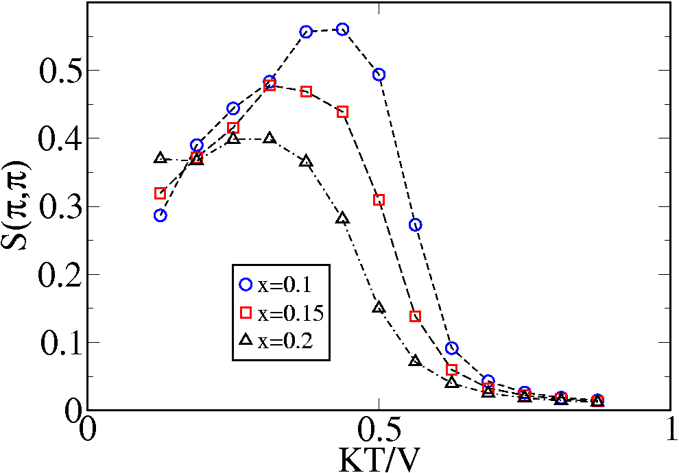
Figure 11: Structure factor vs T (heating run without memory) for different $x$, fixed Monte Carlo steps/spin=1000.

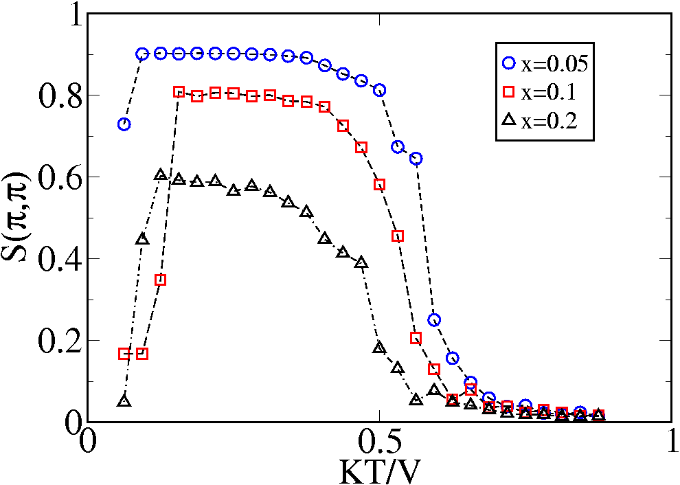
Figure 12: Structure factor vs T (heating run with memory) for different $x$, fixed Monte Carlo steps/spin=1000.

Fig.13, left, shows a low temperature configuration in a well equilibriated sample for 2:1 proportion of B:B’ species. The ordering is disturbed by the occurence of large antisite patches, forced by the excess B. However, the species which occurs in the lesser proportion is found to order as much as possible, and does not form nearest neighbours. In this ‘phase-colouring’ scheme, the antisite regions show up as checkerboard patterns. The actual Fe-Mo checkerboad regions, on the other hand, shows up as domains of a particular colour. The black and white domains are out of phase with respect to each other, while they are separated by thick ’antisite walls’.

Fig.13, right, shows the configuration for B:B’=3:1, the concentration at which the ordering all but disappears. It is observed that the antisite patches have started percolating at this concentration.

  

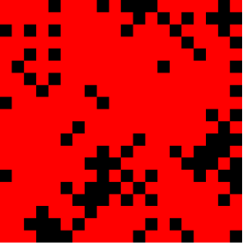
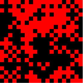
Figure 13: Left: Equilibrium low T (=0.5) configuration for large MCsteps=5000, Fe:Mo=2:1 (x=0.33). Right: Equilibrium low T (=0.5) configuration for large MC steps=5000, Fe:Mo=3:1 (x=0.5).

VII Computational checks

While the previous sections essentially summarize the results for the Fe-Mo ordering problem, it is necessary to probe the sensitivity of the results to the system size and the updating cluster size chosen. In this section, we study these systematics, thereby providing computational indicators to the robustness of our results. In Fig 14 and 15, we plot the dependence of domain sizes on system size and B-B’ ratio. The three columns stand for L=20,40 and 80 from left to right, while the three rows correspond to B-B’ ratio 1:1,1:2 and 1:3 from top to bottom. It is found for all the proportions that the rough domain size remains the same irrespective of the system size, which means that there are more domains for larger system sizes, with more structure to them. This is precisely the reason for the sharp suppression of the nonequilibrium structure factor with increasing system size obseved in Section V.

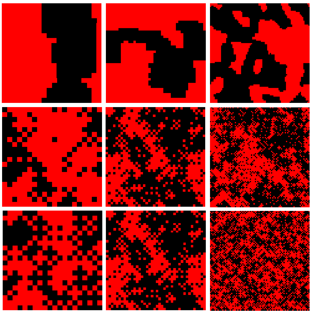
Figure 14: Domain structure for various system sizes: $L=20,~{}40,~{}80$ (left to right) and B:B ratio $1:1,~{}1:2,~{}1:3$ (top to bottom). This is a poorly equilibriated system, with $\tau_{ann}=200$MCS. Notice the increase in antisite disorder with increasing B:B’ disproportionation, and the rough constancy of the typical domain size with increasing $L$.

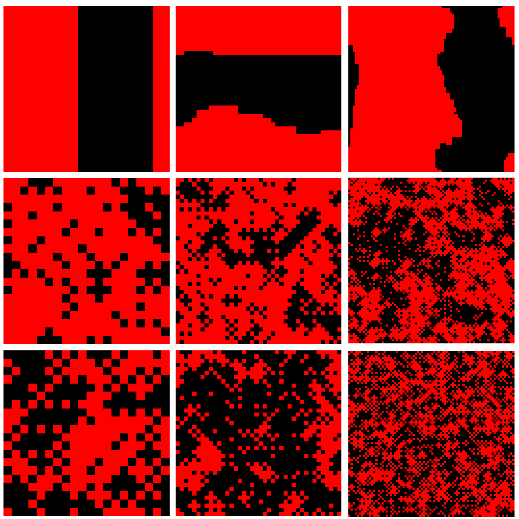
Figure 15: The same as Fig.14, but with much longer equilibriation, $\tau_{ann}=5000$MCS.

The difference between Fig.14 and Fig.15 lies in the fact that the former shows configurations obtained after 200 Monte Carlo steps, while the latter shows configurations obtained by continuing the same run upto 5000 MCS. It is observed that for the case of equal proportions, the domains tend to clump together and become more uniform as the number of MCsteps increase. For the case of different proportions especially Fe:Mo=2:1, i the fraction of antisite defects for lesser MCS is substantially larger than that for greater MCS. This is due to the fact that for MCS=200, there is an extra source of antisite defect formation in addition to the disproportionation, namely insufficient equilibriation. In other words, even the species which occurs in lesser proportion forms nearest neighbours, in contrast to the equilibrium cases of Fig.13. On the other hand, for Fe:Mo=3:1, the inherent disorder due to disproportionation is so large as to mask out the additional nonequilibrium effects.

In Fig.16, the domain pattern is shown for two different update cluster sizes, $L_{c}=4$ (first column) and $L_{c}=10$ (second column). The first row corresponds to 200 MCS, while the second corresponds to 5000 MCS. No appreciable qualitative change is observed, indicating the robustness with respect to this parameter, at least within the regimes considered.

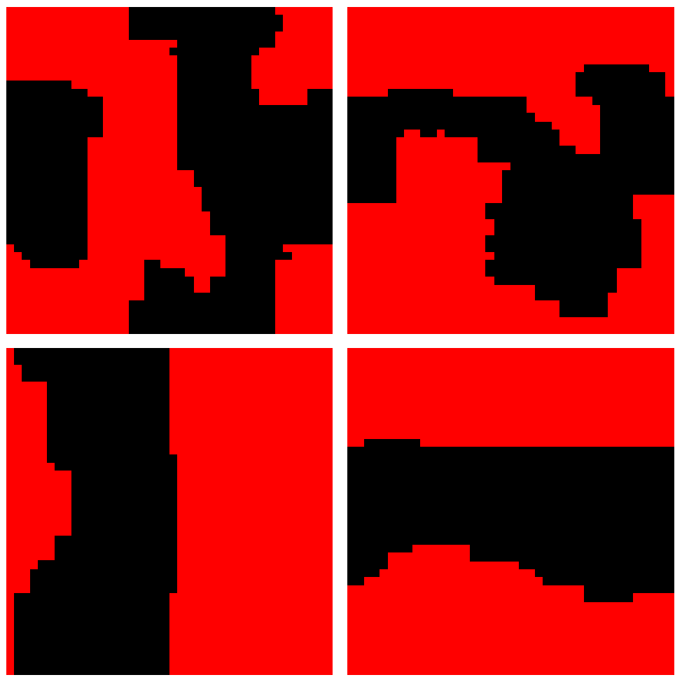
Figure 16: Domain pattern with two different update cluster sizes: 1st column: $L_{C}=4$, 2nd column: $L_{C}=10$. 1st row: 200 MCS, 2nd row: 5000 MCS. $L=40$. The same initial configuration were used as in Fig.14 and Fig.15.

VIII Ordering in ternary B-B’-B” systems

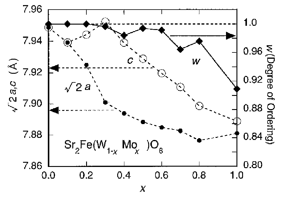
Figure 17: Experimental data on B-B^′ site ordering in Sr₂FeMo_xW_1-xO₆; figure taken from Ref TokuraFeMoW

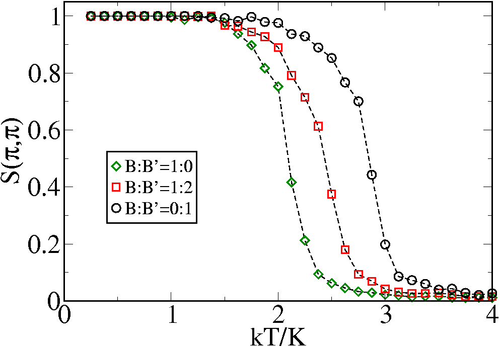
Figure 18: Structure factor vs T (cooling runs) for different Mo-W proportions for the 3species case.

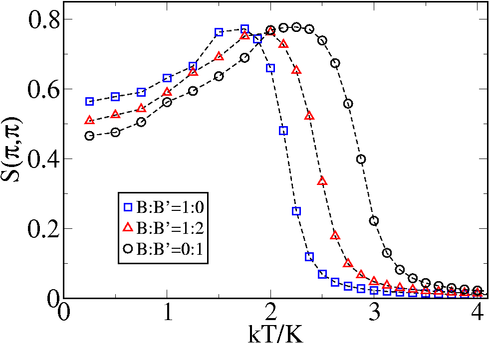
Figure 19: Structure factor vs T (heating without memory) for different Mo-W proportions for a fixed annealing time (2000 MCsteps/spin).

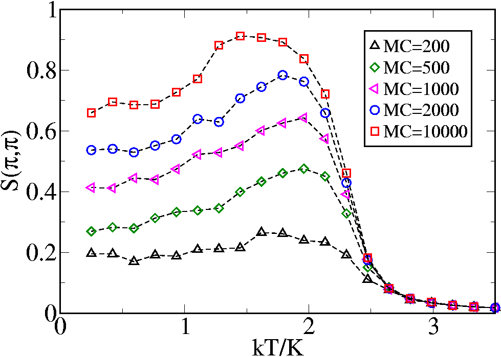
Figure 20: Structure factor vs T (heating without memory) for Mo:W=1:1 for different annealing times.

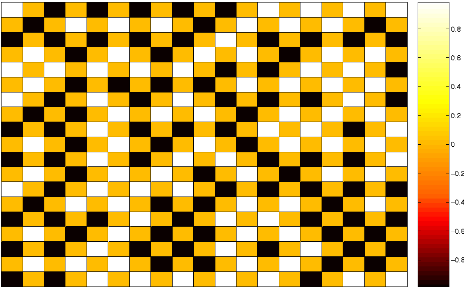
Figure 21: Equilibrium low T configuration for Mo:W=1:1. The black squares represent the Mo, while the white and the yellow represent the W and Fe respectively. Notice perfect B-B’ ordering, but no ordering on the $B^{\prime}$ site between Mo and W.

If Sr₂FeMoO₆ is doped with tungsten to create the series of compounds Sr₂FeMo_xW_1-xO₆, then one has a compositional/structural problem involving three species: Fe, W and Mo. In experiments done by Kobayashi et.al. TokuraFeMoW it was found that the lattice parameters $a$ and $c$ increase with increasing W concentration, indicating a size mismatch. However, the more interesting observation appears to be on the ordering of Fe with respect to Mo/W. Both Kobayashi et. al. and Sarma et.al. SugataFeMoW observed a larger degree of B-B’ ordering in the heavily tungsten doped compounds. The ordering is indeed observed by Kobayashi et. al. to be almost $100\%$ for $x\leq 0.6$, as seen in Fig 17. However, no such ordering is observed on the B’ site for the W and Mo species. Instead, a random mixing of W and Mo is maintained throughout the series.

The above results suggest that there is an effective short range attractive interaction between Fe and either W or Mo, while there is only a much weaker interaction between W and Mo. However, the Fe-W attractive tendency is apparently larger than the Fe-Mo one, since the degree of ordering increases with increasing W concentration. Hence, we model this three-species annealing problem in the following manner.

We consider a site-variable $S$ which can take three possible values: 0 (Fe), 1 (W) and -1 (Mo). Then, we consider the following model hamiltonian:

$$H_{eff}=\sum_{<ij>}[JS_{i}S_{j}+KS_{i}^{2}S_{j}^{2}+L(S_{i}^{2}S_{j}+S_{j}^{2}S_{i})]$$ (6)

This model, a variant of the Blume-Emery-Griffiths model Blume , is a generalization of the Ising model to spin $S=1$ rather than 1/2. One can reduce this model to an effective Ising model in the binary limits of (Fe,Mo), (Fe,W) and (Mo,W), with effective exchange couplings given by $J+K-2L$, $J+K+2L$ and $J$ respectively. Motivated by the experimental observations, we choose the values of the parameters $J,K$ and $L$ such that the effective energy scale for Fe-W ordering is somewhat larger than the Fe-Mo scale, both being substantially large compared to the Mo-W ordering scale. With such a parameter choice, a Monte Carlo is performed as before, and the extent of B-B’ site ordering (not distinguishing between Mo and W on the B’ site, is again quantified by the structure factor at $\{\pi,\pi\}$. The variation of this structure factor with temperature for different relative Mo-W concentrations is plotted in Fig. 18 for cooling runs. The extreme W-only case of course exhibits the highest $T_{c}$ while the Mo-only case shows the lowest one, as expected. For intermediate Mo-W concentrations, the $T_{c}$ for the 3-species assembly interpolates between the two limits. Hence, if one assumes that one has annealed the sample long enough to reach equilibriation at any specific annealing temperature, the B-B’ ordering increases uniformly with increasing W concentration, as observed in the experiment. However, it is interesting to note that the behaviour gets reversed in the off-equilibrium non-monotonic case, as observed in our result for heating run without memory given in Fig. 19. This is because, at any given low temperature, the activation probability for the lowest $T_{c}$ compound is the highest, while that with the highest $T_{c}$ is the lowest. Hence, the compound with the lowest $T_{c}$ reaches equilibrium fastest. This is the reason for the reversal. For completenes, the heating run without memory data is also shown in Fig. 20 for different annealing times, keeping the Mo-W proportion fixed at 1:1. The same transition from non-monotonic to montonic behaviour is observed in this case also. Finally, Fig. 21 shows a ground state equilibrium configuration for Mo:W=1:1 obtained from a cooling run. It is observed that there is perfect ordering on the B site, corresponding to the Fe sublattice. On the B’ site, Mo and W compete for space. There appears to be no significant ordering amongst these latter. Hence, overall this simulates the experimental situation for Sr₂FeMo_1-xW_xO₆ quite effectively.

IX Conclusion

We have shown that antisite disorder can occur due to three reasons: (i) insufficient annealing at low temperatures leading to non-equilibrium configurations, (ii) sufficient annealing leading to equilibrium configurations but at high temperatures close to the order-disorder transition, and (iii) sufficient annealing leading to equilibrium configurations at low temperature, but with different concentrations for the B and the B’ species.

Acknowledgements: We thank D. D. Sarma for introducing us to this problem and several discussions. We also thank Sugato Ray, Anamitra Mukherjee, and Sanjeev Kumar for discussions. We acknowledge use of the Beowulf Cluster at HRI.

X Appendix

We provide the mapping between the lattice gas model and the Blume-Emery-Griffiths model here. If we represent a three-component lattice gas of species A,B and C using spin S=1, with components 1,0,-1, then the number of atoms of each type is given by:

$$N_{A} = \frac{1}{2}\sum_{i=1}^{N}(S_{i}^{2}+S_{i})$$ (7)

$$N_{B} = \frac{1}{2}\sum_{i=1}^{N}(S_{i}^{2}-S_{i})$$ (8)

$$N_{C} = \sum_{i=1}^{N}(1-S_{i}^{2})$$ (9)

An effective spin model can be written as:

$$H=\sum_{ij}[JS_{i}S_{j}+KS_{i}^{2}S_{j}^{2}+L(S_{i}^{2}S_{j}+S_{j}^{2}S_{i})]$$ (10)

where the three parameters $J,K,L$ above are related to the 6 interspecies nearest neighbour interactions by:

$$J = E_{AA}/4+E_{BB}/4-E_{AB}/2$$ (11)

$$K = E_{AA}/4+E_{BB}/4+E_{CC}+E_{AB}/2-E_{AC}-E_{BC}$$ (12)

$$L = E_{AA}/4-E_{BB}/4-E_{AC}/2+E_{BC}/2$$ (13)

It is to be noticed that the relation between the ‘Ising’ parameter $J$ with the energies involve only the A and B species, and is identical to the corresponding relation for the binary alloy case. The explicit relation between the Ising parameter J and the lattice gas parameter $V$ is given by $V=4J$ provided the bonds are counted only once (i.e., the summation over $i,j$ is restricted to $i<j$). Hence, in terms of a lattice gas model, the three parameters $E_{AA},E_{BB}$ and $E_{AB}$ can be expressed in terms of a single parameter:

$$V=(E_{AA}+E_{BB}-2E_{AB})$$

.

References

- (1) D.D. Sarma, Current Op. Solid St. Mat. Sci.,5, 261 (2001).
- (2) T.H. Kim, M. Uehara, S. W. Cheong and S. Lee, Appl. Phys. Lett.,74, 1737 (1999).
- (3) B. Martinez, J. Navarro, Ll. Balcells and J. Fontcuberta, J. Phys.: Condens. Matter 12, 10515 (2000).
- (4) B. Garcia Landa et al, Solid State Comm., 110, 435 (1999).
- (5) K.-I. Kobayashi, T. Kimura, H. Sawada, K. Terakura and Y. Tokura, Nature 395, 677 (1998).
- (6) D. Chaudhuri and D. Stauffer, Principles of Equilibrium Statistical Mechanics
- (7) D.D. Sarma, S. Ray, K. Tanaka, M. Kobayashi, A. Fujimori, P. Sanyal, H.R. Krishnamurthy and C. Dasgupta, Phys. Rev. Lett.,98, 157205 (2007).
- (8) D. Topwal, D.D. Sarma, H. Kato, Y. Tokura and M. Avignon, Phys. Rev. B., 73, 094419 (2006)
- (9) K.-I. Kobayashi, T. Okuda, Y. Tomioka,T. Kimura and Y.Tokura, J. Magn. Magn. Mat., 218, 17 (2000).
- (10) S. Ray, A. Kumar, S. Majumdar, E.V. Sampathkumaran, D.D. Sarma, J. Phys.: Condens. Matter 13, 607 (2001).
- (11) Mukamel and Blume, Phys. Rev. A, 10, 610 (1974).