Geometry of plane sections
of the infinite regular skew polyhedron $\{4,6\,|\,4\}$

Abstract

The asymptotic behavior of open plane sections of triply periodic surfaces is dictated, for an open dense set of plane directions, by an integer second homology class of the three-torus. The dependence of this homology class on the direction can have a rather rich structure, leading in special cases to a fractal. In this paper we present in detail the results for the skew polyhedron $\{4,6\,|\,4\}$ and in particular we show that in this case a fractal arises and that such a fractal can be generated through an elementary algorithm, which in turn allows us to verify for this case a conjecture of S.P.Novikov that such fractals have zero measure.

1 Introduction

The study of plane sections of triply periodic surfaces in $\mathbb{R}^{3}$ was initiated by S.P.Novikov in [Nov82] who raised a question whether open (unbounded) components of such a section have some nice asymptotic behavior. This was motivated by an application to conductivity theory. A number of general theoretical results has been obtained since then by A.Zorich [Zor84], I.Dynnikov [Dyn97, Dyn99], and R.DeLeo [DeL04, DeL05]. For a number of surfaces, R.DeLeo performed a numerical simulation, which confirmed the general conclusions of the theory [DeL03].

In [DeL06] the main results were generalized to polyhedra. Among the class of piecewise linear triply periodic closed surfaces, the one of infinite skew polyhedra [Cox37] is the most suitable for numerical explorations of the geometry of plane sections. In [DeL06] the case of the regular skew polyhedron ${\cal P}$ of type $\{6,4\,|\,4\}$ was studied numerically in detail, showing that the dependence of open section’s asymptotics on the plane direction keeps its rich fractal-like structure also in the piecewise linear case.

In this work we present the results for the dual of ${\cal P}$, namely the cubic polyhedron ${\cal C}=\{4,6\,|\,4\}$ [CGS03]; note that both ${\cal P}$ and ${\cal C}$ are rough PL-approximations of the smooth surface $\{\cos x^{1}+\cos x^{2}+\cos x^{3}=0\}$, which was itself studied numerically in [DeL03]. It turns out that the ${\cal C}$ case is rather noteworthy because its correspondent fractal can be generated recursively through a simple algorithm, which, on one hand, allowed us, for the first time, to verify, in this concrete case, the conjecture [NM03] that the set of exceptional directions has zero measure, and, on the other hand, made possible a systematic comparison with the numerical data obtained through the NTC software library [DeL99].

2 Topological structure of plane sections of triply periodic surfaces

Let $M\subset{\mathbb{T}}^{3}$ be an embedded closed null homologous surface in the torus ${\mathbb{T}}^{3}$, $H=(h_{1},h_{2},h_{3})\in(\mathbb{R}^{3})^{*}$ a covector. We denote by $\widehat{M}$ the preimage of $M$ under the projection $\mathbb{R}^{3}\rightarrow{\mathbb{T}}^{3}=\mathbb{R}^{3}/\mathbb{Z}^{3}$. We consider the sections of $M$ by planes $\langle H,x\rangle=\mathrm{const}$ (we call them $H$-sections) and we are interested in the asymptotical behavior of their unbounded regular connected components (if any). Since only the direction of covector $H$ matters, sometimes we shall treat $H$ as a point of the projective plane $\mathbb{R}{\mathrm{P}}^{2}$.

In studying this question, the foliation $\mathcal{F}_{H}$ induced on $M$ by the closed one-form $\omega=(h_{1}dx^{1}+h_{2}dx^{2}+h_{3}dx^{3})|_{M}$ plays the crucial role. It is well known that, with probability $1$, in a proper sense, a smooth closed one-form whose critical points are all saddles induce dense leaves on $M$. However, by restricting attention to a special class of one-forms that are pull-backs of a constant one-form on ${\mathbb{T}}^{3}$, we fall exactly in the opposite situation, namely, with probability $1$, open leaves are either absent or confined to genus one minimal components of the foliation on $M$, and dense leaves arise only in exceptional cases.

There are three principally different types of foliations $\mathcal{F}_{H}$ and corresponding $H$-sections that may arise, which we call trivial, integrable, and chaotic. Most typically, trivial means that all regular leaves of $\mathcal{F}_{H}$ are closed, integrable means that minimal components of $\mathcal{F}_{H}$ filled with open leaves are of genus one, and in the chaotic case there is a minimal component of genus $>1$. More precise definitions are as follows.

Let $N\subset\mathbb{T}^{3}$ be a piece-wise smooth embedded surface in $\mathbb{T}^{3}$ such that $N\setminus M$ consists of disjoint open disks each of which lies in a plane of the form $\{x\in\mathbb{R}^{3}\;;\;\langle H,x\rangle=\mathrm{const}\}$. Such a surface is obtained by, first, cutting $M$ along some closed null homologous leaves of $\mathcal{F}_{H}$ or null homologous saddle connection cycles, second, removing some of the obtained connected components, and then gluing up planar disks in order to obtain a closed surface. For such a surface $N$, any leaf of $\mathcal{F}_{H}$ is either contained in $N$ or disjoint from $N$. In the former case we say that the leaf is absorbed by $N$. When saying this we shall assume that $N$ is of the just specified form.

Trivial case.

Every leaf of $\mathcal{F}_{H}$ is absorbed by a two-sphere or a null homologous two-torus. If covector $H$ is totally irrational, i.e., $\dim_{\mathbb{Q}}\langle h_{1},h_{2},h_{3}\rangle=3$, then this just means that all connected components of all $H$-sections of $M$ are compact. If $\dim_{\mathbb{Q}}\langle h_{1},h_{2},h_{3}\rangle<3$, then, additionally, periodic, i.e., invariant under a non-trivial shift, unbounded component of $H$-sections may arise;

Integrable case.

Every leaf of $\mathcal{F}_{H}$ is absorbed by a sphere or a two-torus, and at least one leaf is absorbed by a two-torus with non-zero homology class. In this case, every regular non-closed component of an $H$-section is a finitely deformed straight line, i.e., it has the form $\gamma(t)=t\cdot v+O(1)$ for some parametrization, where $v$ is a non-zero vector. If $\dim_{\mathbb{Q}}\langle h_{1},h_{2},h_{3}\rangle=3$, then the non-zero homology class of the tori absorbing leaves of $\mathcal{F}_{H}$ is uniquely defined up to sign. We denote it by $L_{M,H}$ and consider as an integral covector in $\mathbb{R}^{3}$. The identification of $H_{2}(\mathbb{T}^{3},\mathbb{R})$ and $(\mathbb{R}^{3})^{*}=H^{1}(\mathbb{T}^{3},\mathbb{R})$ is given by the Poincare duality. This covector must obviously vanish at vector $v$: $\langle L_{M,H},v\rangle=0$. So, if we assume our three-space Euclidean, then (unless $H$ and $L_{M,H}$ are colinear) we can simply write $v=L_{M,H}\times H$. If $\dim_{\mathbb{Q}}\langle h_{1},h_{2},h_{3}\rangle<3$ the covector $L_{M,H}$ may not be uniquely defined (up to sign), but there may be at most two different choices. We denote the projective class $(L_{1}:L_{2}:L_{3})\in\mathbb{Q}\mathrm{P}^{2}$ of $L_{M,H}$ by $\ell_{M,H}$ and call the soul of the foliation $\mathcal{F}_{H}$.

Chaotic case.

None of the above. If $\dim_{\mathbb{Q}}\langle h_{1},h_{2},h_{3}\rangle=3$, this means that a minimal component of $\mathcal{F}_{H}$ has genus $\geqslant 3$. The behavior of the corresponding $H$-sections have not been studied, but the known examples suggest that, typically, a chaotic $H$-section contains a single unbounded curve that “wonders all around the plane”, i.e., a $d$-neighborhood of the curve is the whole plane for some finite $d$.

For a fixed surface $M$ and a rational point $\ell\in\mathbb{Q}\mathrm{P}^{2}\subset\mathbb{R}\mathrm{P}^{2}$ we denote by ${\cal D}_{M,\ell}$ the set

$${\cal D}_{M,\ell}=\{H\in\mathbb{R}\mathrm{P}^{2}\;;\;\ell_{M,H}=\ell\}.$$

If $\ell_{M,H}$ is not uniquely defined then the point $(h_{1}:h_{2}:h_{3})$ is attributed to both corresponding subsets. The set of points $(h_{1}:h_{2}:h_{3})$ such that the $H$-sections of $M$ are chaotic will be denoted by ${\cal E}(M)$.

The following three propositions are extracted from [Dyn99].

Proposition 1.

For a generic surface $M\subset\mathbb{T}^{3}$ the sets ${\cal D}_{M,\ell}$ are disjoint closed domains with piece-wise smooth boundary. The set ${\cal E}(M)$ is disjoint from $\mathbb{Q}\mathrm{P}^{2}$ and has zero measure. The set of directions $H$ with trivial $H$-sections is open.

In other words, the first claim of this proposition says that $\ell$, where defined, is a locally constant function of $H$. We call the non-empty domains ${\cal D}_{M,\ell}$ stability zones and refer to $\ell$ as the label of the stability zone ${\cal D}_{M,\ell}$.

For studying the stability zones, it is usefull to consider a 1-parametric family $M_{c}=\{x\in\mathbb{T}^{3}\;;\;f(x)=c\}$ of level surfaces of a fixed smooth function.

Proposition 2.

For a generic function $f$, there are continuous functions $e_{1},e_{2}:\mathbb{R}{\mathrm{P}}^{2}\rightarrow\mathbb{R}$ such that

• $e_{1}(H)\leqslant e_{2}(H)$ for all $H\in\mathbb{R}{\mathrm{P}}^{2}$;

• the $H$-sections of $M_{c}$ are trivial if and only if $c\notin[e_{1}(H),e_{2}(H)]$;

• if $e_{1}(H)<e_{2}(H)$, then the $H$-sections of $M_{c}$ are integrable for all $c\in[e_{1}(H),e_{2}(H)]$, and the soul $\ell$ of the corresponding foliation $\mathcal{F}_{c,H}$ is independent of $c$.

We define generalized stability zones ${\cal D}_{f,\ell}$ as $\mathcal{D}_{f,\ell}=\cup_{c}\mathcal{D}_{M_{c},\ell}$, and the set ${\cal E}(f)$ as ${\cal E}(f)=\cup_{c}{\cal E}(M_{c})$.

Proposition 3.

For a generic $f$, generalized stability zones are closed domains with piece-wise smooth boundary. If $\ell\neq\ell^{\prime}$ then the zones $\mathcal{D}_{f,\ell}$ $\mathcal{D}_{f,\ell^{\prime}}$ can only have intersections at the boundary, and, moreover, the number of their common points is at most countable. If the whole $\mathbb{R}{\mathrm{P}}^{2}$ is not covered by a single generalized stability zone, then the number of zones is countably infinite, and the set ${\cal E}(f)=\mathbb{R}{\mathrm{P}}^{2}\setminus(\cup_{\ell}{\cal D}_{f,\ell})$ is non-empty and uncountable.

It may happen that there is just one generalized stability zone (say, a small enough perturbation of the function $\sin(x^{1})$ will work), but it is also easy to find a function $f$ with non-empty ${\cal E}(f)$: any function with cubical symmetry is such. In all examples known to us two different generalized stability zones have at most one point in common.

It follows from Propositions 1–3 that the union $\cup_{\ell\in\mathbb{Q}\mathrm{P}^{2}}\text{int}(\mathcal{D}_{f,\ell})$ of the interiors of the zones is an open everywhere dense subset of $\mathbb{R}\mathrm{P}^{2}$ and its complement $\overline{\mathcal{E}(f)}$ has the form of a two-dimensional cut out fractal set.

Proposition 4 ([DeL04]).

If there is more than one generalized stability zone, then $\overline{\mathcal{E}(f)}$ is the set of accumulation points of the set of their souls.

It is plausible but still unknown whether $\mathcal{E}(f)$ has always zero measure. The following stronger conjecture was proposed in [NM03].

Conjecture.

Whenever ${\cal E}(f)$ is non-empty, the Hausdorff dimension of ${\cal E}(f)$ is strictly between 1 and 2 for every $f$.

So far only numerical checks of this conjecture were available in the literature [DeL03, DeL06]; in the next sections we shall provide, for the particular case of the polyhedron ${\cal C}$, a full proof of the weaker, zero measure, conjecture and good numerical evidence for the stronger one.

3 Stability zones of ${\cal C}$

The regular skew polyhedron ${\cal C}=\{4,6\,|\,4\}$ (see Figure 1) is, up to isometries, the unique cubic polyhedron with all monkey-saddle vertices [CGS03]; the vertices of its embedding in ${\mathbb{T}}^{3}=[0,1]^{3}/\sim$ are the eight points in the orbit of $P=(1/4,1/4,1/4)$ under the cubic symmetry group. As level surface, ${\cal C}$ can be represented in the $[0,1]^{3}$ cube as $\theta^{-1}(0)$ for

$$\theta(x^{1},x^{2},x^{3})=\hbox{mid}(|2x^{1}-1|,|2x^{2}-1|,|2x^{3}-1|)-\frac{1}{2},$$

where $\hbox{mid}(a,b,c)$ is the middle value among $a$, $b$, and $c$.

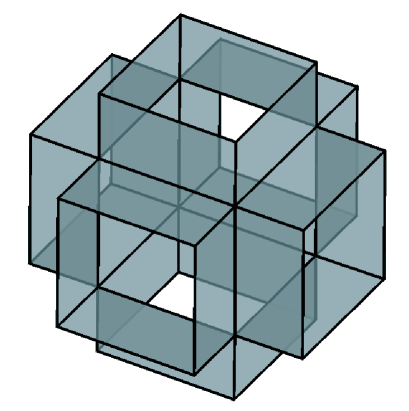
Figure 1: The $\{4,6\,|\,4\}$ polyhedron embedded in the three-torus. Shown is the fundamental domain, which lies in the $[0,1]^{3}$ cube.

This surface, as well as the surface $\cos x^{1}+\cos x^{2}+\cos x^{3}=0$ and ${\cal C}$’s dual—the truncated octahedron, has a very strong symmetry, namely, its exterior is equal to its interior modulo a translation. This means that for $\theta$ the functions $e_{1,2}$ mentioned in Propositoin 2 are such that $e_{1}=-e_{2}$, and hence, stability zones of the surface ${\cal C}$ coincide with generalized stability zones of the function $\theta$.

Let us denote by $\psi_{1},\psi_{2},\psi_{3}$ the following projective transformations:

$$\psi_{1}(h_{1}:h_{2}:h_{3}) =(h_{1}:h_{2}+h_{1}:h_{3}+h_{1}),$$

$$\psi_{2}(h_{1}:h_{2}:h_{3}) =(h_{1}+h_{2}:h_{2}:h_{3}+h_{2}),$$

$$\psi_{3}(h_{1}:h_{2}:h_{3}) =(h_{1}+h_{3}:h_{2}+h_{3}:h_{3}).$$

Theorem 1.

For the surface ${\cal C}$ the stability zones are as follows:

$$\mathcal{D}_{(1:0:0)}({\cal C}) =\{(h_{1}:h_{2}:h_{3})\in\mathbb{R}\mathrm{P}^{2}\;;\;h_{1}\geqslant\left|h_{2}\right|+\left|h_{3}\right|\},$$

$$\mathcal{D}_{(1:1:1)}({\cal C}) =\{(h_{1}:h_{2}:h_{3})\in\mathbb{R}\mathrm{P}^{2}\;;\;\left|h_{1}\right|+\left|h_{2}\right|+\left|h_{3}\right|\leqslant 4h_{1},4h_{2},4h_{3}\},$$

$$\mathcal{D}_{\psi_{i_{1}}(\psi_{i_{1}}(\ldots\psi_{i_{k}}((1:1:1))\ldots))}({\cal C}) =\psi_{i_{1}}(\psi_{i_{1}}(\ldots\psi_{i_{k}}(\mathcal{D}_{(1:1:1)}({\cal C}))\ldots)),$$

where $(i_{1},\ldots,i_{k})$ is an arbitrary finite sequence of elements from $\{1,2,3\}$, and, in addition, all zones obtained from the listed ones by cubical symmetries: permutations and changing signs of the coordinates.

The proof of this theorem will rest on the following two lemmas.

Lemma 1.

We have

$$\mathcal{D}_{(1:0:0)}({\cal C})\supset\{(h_{1}:h_{2}:h_{3})\in\mathbb{R}\mathrm{P}^{2}\;;\;h_{1}\geqslant\left|h_{2}\right|+\left|h_{3}\right|\}.$$

Proof.

If the inequality $h_{1}\geqslant\left|h_{2}\right|+\left|h_{3}\right|$ is satisfied then the plane $h_{1}x^{1}+h_{2}x^{2}+h_{3}x^{3}=\mathrm{const}$ passing through the center of the unit cube $[0,1]^{3}$ separates the faces $x^{1}=0$ and $x^{1}=1$. This means that closed leaves of the corresponding foliation will cut our triply periodic surface $\widehat{\cal C}$ into parts each of which is a finitely deformed plane $x^{1}=\mathrm{const}$ with holes (see Figure 2). Filling the holes by flat disks and projecting to $\mathbb{T}^{3}$ we obtain two tori whose homology class is equal up to sign to $(1,0,0)\in(\mathbb{R}^{3})^{*}$. ∎

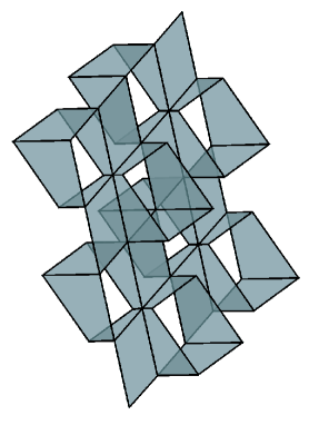
Figure 2: A connected component of $\widehat{\cal C}$ after cutting along closed leaves

Lemma 2.

Let $h_{1},h_{2},h_{3}\geqslant 0$, $(h_{1},h_{2},h_{3})\neq(0,0,0)$. Then we have $(h_{1}:h_{2}:h_{3})\in\mathcal{D}_{\ell}$ if and only if $\psi_{i}((h_{1}:h_{2}:h_{3}))\in\mathcal{D}_{\psi_{i}(\ell)}$, where $i=1,2,3$.

Proof.

For convenience, we shift the coordinate system as follows: $(x^{1},x^{2},x^{3})\mapsto(x^{1}+1/4,x^{2}+1/4,x^{3}+1/4)$. Our surface $\widehat{\cal C}$ cuts $\mathbb{R}^{3}$ into two parts, $N_{-}$ and $N_{+}$, that can now be characterized as follows: $N_{-}$ (resp. $N_{+}$) consists of points $(x^{1},x^{2},x^{3})\in\mathbb{R}^{3}$ such that at least two (resp. at most one) of the three numbers $\{x^{1}\},\{x^{2}\},\{x^{3}\}$ are in the interval $[0,1/2]$ (resp. $(0,1/2)$), where $\{x\}$ denotes the fractional part of $x$.

We may assume $i=3$, $(h_{1},h_{2},h_{3})=(\alpha,\beta,1)$ without loss of generality. Let $\Pi$ be the plane defined by $\alpha x^{1}+\beta x^{2}+x^{3}=c$. Denote by $Q_{-}$ the projection of $\Pi\cap N_{-}$ to the $x^{1},x^{2}$-plane along $x^{3}$. According to the description of $N_{-}$ given above $Q_{-}$ is the set of points $(x^{1},x^{2})\in\mathbb{R}^{2}$ such that exactly two of the three numbers $\{x^{1}\},\{x^{2}\},\{c-\alpha x^{1}-\beta x^{2}\}$ are in the interval $[0,1/2]$.

Denote by $\square_{a,b}$ the square $\{(x^{1},x^{2})\in\mathbb{R}^{2}\,;\,a\leqslant x^{1}\leqslant a+1/2,\,b\leqslant x^{2}\leqslant b+1/2\}$, and by $S_{m}$ the strip defined by $m\leqslant c-\alpha x^{1}-\beta x^{2}\leqslant m+1/2$. We have

$$Q_{-}=\Bigl{(}\bigcup_{j,k\in\mathbb{Z}}\square_{j,k}\Bigr{)}\cup\Bigl{(}\bigcup_{j,k,m\in\mathbb{Z}}\square_{j+1/2,k}\cap S_{m}\Bigr{)}\cup\Bigl{(}\bigcup_{j,k,m\in\mathbb{Z}}\square_{j,k+1/2}\cap S_{m}\Bigr{)}.$$

The first part in this union, $\bigcup_{j,k\in\mathbb{Z}}\square_{j,k}$, does not depend on $\Pi$. We call these squares mainlands.

Each intersection $\square_{j+1/2,k}\cap S_{m}$ with $j,k,m\in\mathbb{Z}$, whenever non-empty, is a convex polygon that can be of the following three types:

cape:

it has a piece of boundary in common with exactly one of the mainlands $\square_{j,k}$ or $\square_{j+1,k}$;

bridge:

it has a piece of boundary in common with both mainlands $\square_{j,k}$ and $\square_{j+1,k}$;

island:

it is disjoint from mainlands.

Similarly, one defines the type of a polygon $\square_{j,k+1/2}\cap S_{m}$ regarding adjacency to the mainlands $\square_{j,k}$ and $\square_{j,k+1}$, see Figure 3.

Figure 3: Geography of the section $\Pi\cap N_{-}$

Capes are not interesting for us because their removal is equivalent to a finite deformation of $Q_{-}$. It is not hard to write the necessary and sufficient condition for $\square_{j+1/2,k}\cap S_{m}$ to be a bridge:

$$c-\alpha\Bigl{(}j+\frac{1}{2}\Bigr{)}-\beta\Bigl{(}k+\frac{1}{2}\Bigr{)}-\frac{1}{2}\leqslant m\leqslant c-\alpha(j+1)-\beta k,$$ (1)

or an island:

$$c-\alpha\Bigl{(}j+\frac{1}{2}\Bigr{)}-\beta\Bigl{(}k+\frac{1}{2}\Bigr{)}-\frac{1}{2}\geqslant m\geqslant c-\alpha(j+1)-\beta k.$$ (2)

Now we apply $\psi_{3}$ to $H$, which gives $H^{\prime}=(\alpha^{\prime},\beta^{\prime},1)=(\alpha+1,\beta+1,1)$. Let $Q_{-}^{\prime}$ and $S_{m}^{\prime}$ be defined in the same way as $Q_{-}$ and $S_{m}$ with $\alpha$ and $\beta$ replaced by $\alpha^{\prime}=\alpha+1$ and $\beta^{\prime}=\beta+1$, respectively. Then the intersection $\square_{j+1/2,k}\cap S_{m}^{\prime}$ is a bridge if and only if

$$c-(\alpha+1)\Bigl{(}j+\frac{1}{2}\Bigr{)}-(\beta+1)\Bigl{(}k+\frac{1}{2}\Bigr{)}-\frac{1}{2}\leqslant m\leqslant c-(\alpha+1)(j+1)-(\beta+1)k,$$

which can be rewritten as

$$c-\alpha\Bigl{(}j+\frac{1}{2}\Bigr{)}-\beta\Bigl{(}k+\frac{1}{2}\Bigr{)}-\frac{1}{2}\leqslant m+j+k+1\leqslant c-\alpha(j+1)-\beta k.$$

Thus, $\square_{j+1/2,k}\cap S_{m}$ is a bridge if and only if so is $\square_{j+1/2,k}\cap S_{m-j-k-1}^{\prime}$. Similarly, the same is true about islands as well as bridges and islands in squares of the form $\square_{j,k+1/2}$.

So, bridges and islands of $Q_{-}^{\prime}$ in the square $\square_{j+1/2,k}$ or $\square_{j,k+1/2}$ are in a natural one to one correspondence with those of $Q_{-}$. Therefore, $Q_{-}^{\prime}$ and $Q_{-}$ are obtained from each other by a finite deformation. The geometrical difference between $Q_{-}^{\prime}$ and $Q_{-}$ can be vaguely described as follows: islands and bridges of $Q_{-}^{\prime}$ are narrower than those of $Q_{-}$, and $Q_{-}^{\prime}$ has more capes. See Figure 4 for an example.

$$\begin{array}[]{cc}\includegraphics[height=113.81102pt]{grid1.eps}&\includegraphics[height=113.81102pt]{grid2.eps}\\ Q_{-}&Q_{-}^{\prime}\end{array}$$

Figure 4: The transition from $Q_{-}$ to $Q_{-}^{\prime}$ produces more capes and makes the bridges narrower

In the genus three case the integrability of our foliation is equivalent to the existence of closed fibres of the foliation (or null homologous saddle connection cycles). We have just seen that $H$-sections and $H^{\prime}$-sections are obtained from each other by a finite deformation. Hence, they are both integrable or both chaotic. If they are integrable, let $\ell$ and $\ell^{\prime}$ be the labels of the corresponding zones. We want to show that $\ell^{\prime}=\psi_{3}(\ell)$. Since both $\ell$ and $\ell^{\prime}$ are locally constant functions of $H$ it is enough to consider the case of totally irrational $H$. Then the asymptotic direction $v=H\times\ell$ is of irrationality degree two, i.e., $\dim_{\mathbb{Q}}\langle v^{1},v^{2},v^{3}\rangle=2$, and $\ell$ is the only rational covector up to multiple that vanishes at $v$. Thus, it suffices to show that $\psi_{3}(\ell)$ vanishes at $v^{\prime}$, the direction of open components of $H^{\prime}$-sections.

The latter follows easily from the fact that the projections of $v$ and $v^{\prime}$ to the $x^{1},x^{2}$-plane coincide, which, in turn, follows from the coincidence, up to finite deformation, of $Q_{-}$ and $Q_{-}^{\prime}$. ∎

Proof of Theorem 1.

Due to the cubical symmetry of the surface it suffices to establish the fractal structure in the region $C_{+}=\{(h_{1}:h_{2}:h_{3})\in\mathbb{R}\mathrm{P}^{2}\,;\,h_{1},h_{2},h_{3}\geqslant 0\}$. Put

$$\mathcal{R}_{(1:0:0)} =\{(h_{1}:h_{2}:h_{3})\in\mathbb{R}\mathrm{P}^{2}\;;\;h_{1}\geqslant\left|h_{2}\right|+\left|h_{3}\right|\},$$

$$\mathcal{R}_{(0:1:0)} =\{(h_{1}:h_{2}:h_{3})\in\mathbb{R}\mathrm{P}^{2}\;;\;h_{2}\geqslant\left|h_{1}\right|+\left|h_{3}\right|\},$$

$$\mathcal{R}_{(0:0:1)} =\{(h_{1}:h_{2}:h_{3})\in\mathbb{R}\mathrm{P}^{2}\;;\;h_{3}\geqslant\left|h_{1}\right|+\left|h_{2}\right|\},$$

$$\mathcal{R}_{(1:1:1)} =\{(h_{1}:h_{2}:h_{3})\in\mathbb{R}\mathrm{P}^{2}\;;\;\left|h_{1}\right|+\left|h_{2}\right|+\left|h_{3}\right|\leqslant 4h_{1},4h_{2},4h_{3}\},$$

$$\mathcal{R}_{\psi_{i_{1}}(\psi_{i_{1}}(\ldots\psi_{i_{k}}((1:1:1))\ldots))} =\psi_{i_{1}}(\psi_{i_{1}}(\ldots\psi_{i_{k}}(\mathcal{R}_{(1:1:1)})\ldots)),$$

and $\mathcal{R}_{\ell}=\varnothing$ if $\ell\notin\{(1:0:0),(0:1:0),(0:0:1)\}$ and $\ell$ is not of the form $\psi_{i_{1}}(\psi_{i_{1}}(\ldots\psi_{i_{k}}((1:1:1))\ldots))$. We want to show that $\mathcal{R}_{\ell}=\mathcal{D}_{\ell}$ for all $\ell\in\mathbb{Q}\mathrm{P}^{2}\cap C_{+}$. We have already shown in Lemma 1 that $\mathcal{R}_{\ell}\subset\mathcal{D}_{\ell}$ for $\ell=(1:0:0)$ By symmetry it is also true for $\ell=(0:1:0),(0:0:1)$.

It is a straightforward check to see that

$$\mathcal{R}_{(1:1:1)}=\psi_{1}(\mathcal{R}_{(1:0:0)}\cap C_{+})\cup\psi_{2}(\mathcal{R}_{(0:1:0)}\cap C_{+})\cup\psi_{3}(\mathcal{R}_{(0:0:1)}\cap C_{+}).$$

By Lemma 2 this implies $\mathcal{R}_{(1:1:1)}\subset\mathcal{D}_{(1:1:1)}$ as $(1:1:1)=\psi_{1}(1:0:0)=\psi_{2}(0:1:0)=\psi_{3}(0:0:1)$, and, therefore, $\mathcal{R}_{\ell}\subset\mathcal{D}_{\ell}$ for all $\ell\in C_{+}\cap\mathbb{Q}\mathrm{P}^{2}$.

In order to establish Theorem 1 it suffices to show that the zones $\mathcal{D}_{\ell}$ are not larger that $\mathcal{R}_{\ell}$, and there are no other stability zones. Both claims follow from the fact that $\bigcup_{\ell}\mathcal{R}_{\ell}$ covers all rational points:

$$\bigcup_{\ell}\mathcal{R}_{\ell}\supset C_{+}\cap\mathbb{Q}\mathrm{P}^{2}.$$

Indeed, let $\varphi$ be the following map from $C_{+}$ to itself:

$$\varphi(h_{1}:h_{2}:h_{3})=\left\{\begin{aligned} (h_{1}:h_{2}-h_{1}:h_{3}-h_{1})&,\text{ if }0\leqslant h_{1}\leqslant h_{2},h_{3},\\ (h_{2}:h_{3}:h_{1})&,\text{ otherwise}.\end{aligned}\right.$$

By construction, for every $H\in C_{+}$ we have $H\in\bigcup_{\ell}\mathcal{R}_{\ell}$ if and only if $\varphi(H)\in\bigcup_{\ell}\mathcal{R}_{\ell}$. If $H$ is a rational covector from $C_{+}$, then after applying $\varphi$ finitely many times, one of the coordinates of the obtained covector becomes zero. All such points are covered by $\mathcal{R}_{(1:0:0)}$, $\mathcal{R}_{(0:1:0)}$ and $\mathcal{R}_{(0:0:1)}$. ∎

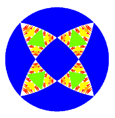
Figure 5: Picture of the fractal in the disc model of ${\mathbb{R}}\hbox{\rm P}^{2}$. The center of the disc corresponds to the $z$ axis, so the central square is the stability zone ${\cal D}_{(0:0:1)}$, the one touching it in the left and right vertices is ${\cal D}_{(1:0:0)}$ and the third one is ${\cal D}_{(0:1:0)}$. The green triangles are the stability zones ${\cal D}_{(1:1:1)}$, ${\cal D}_{(1:1:-1)}$, ${\cal D}_{(1:-1:1)}$ and ${\cal D}_{(1:-1:-1)}$.

So, we have the following picture in $\mathbb{R}\mathrm{P}^{2}$: four lines $h_{1}\pm h_{2}\pm h_{3}=0$ cut $\mathbb{R}\mathrm{P}^{2}$ into three “squares”, which are zones $\mathcal{D}_{(1:0:0)}$, $\mathcal{D}_{(0:1:0)}$, $\mathcal{D}_{(0:0:1)}$, and four triangles obtained from each other by cubical symmetries, in which there are infinitely many stability zones. We shall concentrate on the triangle that is contained in $C_{+}$. This triangle has vertices $(1:1:0)$, $(1:0:1)$, $(0:1:1)$ and is defined by the inequalities

$$\frac{h_{1}+h_{2}+h_{3}}{2}\geqslant h_{1},h_{2},h_{3}\geqslant 0.$$

Let us denote this triangle by $\Delta$. The zone $\mathcal{D}_{(1:1:1)}$ is also a triangle that is contained in $\Delta$ and has its vertices, $(2:1:1)$, $(1:2:1)$, $(1:1:2)$, at the sides of $\Delta$. The complement $\Delta\setminus\mathcal{D}_{(1:1:1)}$ consists of three triangles that are exactly $\psi_{1}(\Delta)$, $\psi_{2}(\Delta)$, and $\psi_{3}(\Delta)$. In each triangle $\Delta_{1}=\psi_{1}(\Delta)$, $\Delta_{2}=\psi_{2}(\Delta)$, $\Delta_{3}=\psi_{3}(\Delta)$ the picture is obtained from that in $\Delta$ by the corresponding projective transformation $\psi_{i}$.

For a finite sequence $a=(a_{1},a_{2},\dots,a_{k})$ of indices $1,2,3$ we denote by $\psi_{a}$ the mapping $\psi_{a_{1}}\circ\psi_{a_{2}}\circ\ldots\circ\psi_{a_{k}}$. By $a^{\prime}$, $a^{\prime\prime}$, and $a^{\prime\prime\prime}$ we denote the sequences $(a_{1},\dots,a_{k},1)$, $(a_{1},\dots,a_{k},2)$, $(a_{1},\dots,a_{k},3)$, respectively. For any such sequence $a$ we have the following. The triangle $\Delta_{a}=\psi_{a}(\Delta)$ is bounded by the zones $\mathcal{D}_{\psi_{a}(1:0:0)}$, $\mathcal{D}_{\psi_{a}(0:1:0)}$, $\mathcal{D}_{\psi_{a}(0:0:1)}$. It contains the zone $\mathcal{D}_{\psi_{a}(1:1:1)}$ whose vertices $\psi_{a}(2:1:1)$, $\psi_{a}(1:2:1)$, $\psi_{a}(1:1:2)$ are on the sides of $\Delta_{a}$, and the complement $\Delta_{a}\setminus\mathcal{D}_{\psi_{a}(1:1:1)}$ is the union of the triangles $\Delta_{a^{\prime}}$, $\Delta_{a^{\prime\prime}}$, $\Delta_{a^{\prime\prime\prime}}$.

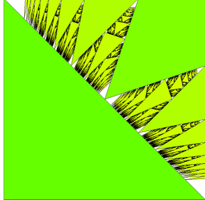
Figure 6: Picture of the fractal in the square $[0,1]^{2}$ in the $z=1$ projective chart.

Proposition 5.

The intersection $\mathcal{E}({\cal C})\cap C_{+}$ consists of points of the form

$$\lim_{k\rightarrow\infty}\psi_{i_{1}}(\psi_{i_{2}}(\ldots\psi_{i_{k}}((1:1:1))\ldots)),$$

where $(i_{1},i_{2},\ldots)$ runs over all possible sequences of elements from $\{1,2,3\}$ containing each index infinitely many times. Other points in $\mathcal{E}({\cal C})$ are obtained from these by cubical simmetries.

Proof.

From the structure of stability zones established above it follows that the intersection $\mathcal{E}\cap C_{+}$ is the union of subsets

$$\bigcap\limits_{k}\psi_{i_{1}}(\psi_{i_{2}}(\ldots\psi_{i_{k}}(\Delta)\ldots))$$

over all sequences $(i_{k})\in 3^{\mathbb{N}}$ in which all three indices appear infinitely many times. It suffices to show that every such a subset is actually a single point, which follows from Proposition 9 below. ∎

3.1 Measure of ${\cal E}$

In all cases studied so far no algorithm was found to generate all stability zones and nothing could be said about the measure of the ${\cal E}(f)$. This is therefore the first case in which it is possible to check the truth of the zero measure conjecture.

Theorem 2.

The set $\mathcal{E}({\cal C})$ of “chaotic” directions has measure zero.

Proof.

Again, due to the symmetry, it suffices to prove the claim for $\mathcal{E}\cap C_{+}$. We denote this set by $\mathcal{E}_{+}$. As we have seen, it is contained in the triangle $\Delta$, and the following holds:

$$\mathcal{E}_{+}=\psi_{1}(\mathcal{E}_{+})\cup\psi_{2}(\mathcal{E}_{+})\cup\psi_{3}(\mathcal{E}_{+}).$$

Applying this recursively, we get

$$\mathcal{E}_{+}=\psi_{1}(\mathcal{E}_{+})\cup\psi_{2}(\mathcal{E}_{+})\cup\psi_{31}(\mathcal{E}_{+})\cup\psi_{32}(\mathcal{E}_{+})\cup\psi_{331}(\mathcal{E}_{+})\cup\psi_{332}(\mathcal{E}_{+})\cup\\ \ldots\cup\psi_{\underbrace{\scriptstyle 3\ldots 3}_{k}1}(\mathcal{E}_{+})\cup\psi_{\underbrace{\scriptstyle 3\ldots 3}_{k}2}(\mathcal{E}_{+})\cup\psi_{\underbrace{\scriptstyle 3\ldots 3}_{k+1}}(\mathcal{E}_{+}).$$ (3)

Let $\mu$ be the measure of $\mathcal{E}_{+}$ and $\mu_{k}$ the measure of $\psi_{\underbrace{\scriptstyle 3\ldots 3}_{k}1}(\mathcal{E}_{+})$, which is equal to the measure of $\psi_{\underbrace{\scriptstyle 3\ldots 3}_{k}2}(\mathcal{E}_{+})$. The measure of the triangle $\psi_{\underbrace{\scriptstyle 3\ldots 3}_{k+1}}(\mathcal{E}_{+})$ tends to zero as $k$ goes to $\infty$. Therefore, we have

$$\mu=2\sum_{k=0}^{\infty}\mu_{k}.$$

The idea now is to show that $\mu_{k}\leqslant c_{k}\mu$, where $c_{0},c_{1},\ldots$ are constants such that

$$\sum_{k=0}^{\infty}c_{k}<\frac{1}{2},$$

which, together with the previous equality, implies $\mu=0$.

Now we provide the necessary technical details. First of all, we need to parametrise the triangle $\Delta$. We use the following parametrization: $(u,v)\mapsto(1-v:1-u:u+v)$, $u,v\geqslant 0$, $u+v\leqslant 1$.

The property of a set to be of zero measure does not depend on the choice of a regular Borel measure. In order to get the desired inequalities we use a somewhat artificial measure on $\Delta$, namely the following one:

$$\frac{du\,dv}{(1+u+v)^{2}}.$$

By doing so we keep the symmetry between $\psi_{1}$ and $\psi_{2}$ (one is conjugate to the other by the permutation $u\leftrightarrow v$), so the measures of the sets $\psi_{\underbrace{\scriptstyle 3\ldots 3}_{k}1}(\mathcal{E}_{+})$ and $\psi_{\underbrace{\scriptstyle 3\ldots 3}_{k}2}(\mathcal{E}_{+})$ coincide. We denote by $f_{k}$ the mapping $\psi_{\underbrace{\scriptstyle 3\ldots 3}_{k}1}\circ R$, where $R(h_{1}:h_{2}:h_{3})=(h_{3}:h_{1}:h_{2})$, written in the $u,v$-parametrization:

$$f_{k}(u,v)=\Bigl{(}\frac{v}{u+(k+1)(v+1)},\frac{1}{u+(k+1)(v+1)}\Bigr{)}.$$

Since we have $R(\mathcal{E})=\mathcal{E}$, the image $f_{k}(\mathcal{E}_{+})$ coincides with $\psi_{\underbrace{\scriptstyle 3\ldots 3}_{k}1}(\mathcal{E}_{+})$.

Obviously, the measure of $f_{k}(\mathcal{E}_{+})$ is bounded from above by $c_{k}\mu$, where

$$c_{k}=\max_{u,v\geqslant 0,\,u+v\leqslant 1}J_{f_{k}}(u,v)\frac{(1+u+v)^{2}}{\Bigl{(}1+\frac{v}{u+(k+1)(v+1)}+\frac{1}{u+(k+1)(v+1)}\Bigr{)}^{2}}.$$

By $J_{f}$ we denote the Jacobian of the mapping $f$. A routine check gives:

$$c_{k}=\max_{u,v\geqslant 0,\,u+v\leqslant 1}\frac{(1+u+v)^{2}}{(u+(k+2)(v+1))^{2}(u+(k+1)(v+1))}=\\ \left\{\begin{array}[]{ll}\displaystyle\frac{1}{4}&\text{if }k=0,\\ \displaystyle\frac{4}{(k+2)(k+3)^{2}}&\text{otherwise},\end{array}\right.$$

$$\sum_{k=0}^{\infty}c_{k}=\frac{1}{4}+\sum_{k=1}^{\infty}\frac{4}{(k+2)(k+3)^{2}}=\frac{253}{36}-\frac{2}{3}\pi^{2}\approx 0.448<\frac{1}{2},$$

which completes the proof.

∎

3.2 Asymptotics of stability zones and fractal dimension of ${\cal E}$

From what said at the beginning of the section it follows immediately that all stability zones, except the biggest ones, which are squares, are triangles and their labels satisfy a simple recursive relation.

Proposition 6.

Every stability zone of ${\cal C}$, except for the three squares with souls $(1:0:0)$, $(0:1:0)$, and $(0:0:1)$, are triangles; these triangles are generated starting from $\Delta$ (and its three symmetric triangles with respect to the coordinate planes) according to the the following recursive algorithm:

1. evaluate the vector sums $w_{1}=v_{2}+v_{3}$, $w_{2}=v_{3}+v_{1}$, $w_{3}=v_{1}+v_{2}$ of all pairs of the three vertices $v_{i}$ of $\Delta$;

2. consider the $w_{i}$ as projective coordinates and add the triangle having those points as vertices to the list of all stability zones – its soul is given by the vector sum of the three vertices of $\Delta$;

3. consider now the three triangles $\Delta_{1}=\langle v_{1},w_{2},w_{3}\rangle$, $\Delta_{2}=\langle w_{1},v_{2},w_{3}\rangle$, $\Delta_{3}=\langle w_{1},w_{2},v_{3}\rangle$ and repeat the algorithm for each of them.

This fact can be exploited to find an explicit expression for elements of ${\cal E}$ by considering “spiralling down” (or “steepest descent”) sequences of stability zones (see Figure 7). Select indeed an ordered triple $(\alpha,\beta,\gamma)$ of stability zones which bind a triangle, namely such that two touch each other and the third touches both, and build out of them the recursive sequence of stability zones such that every new stability zone is the one whose vertices touch the previous three stability zones. It is easy to see that the sequence of these stability zones are arranged in a sort of spiral and by construction, the label of every stability zone of this sequence is the sum of the labels of the previous three zones, so that the sequence of the labels is a Tribonacci sequence in $\mathrm{P}H_{2}({\mathbb{T}}^{3},{\mathbb{Z}})$.

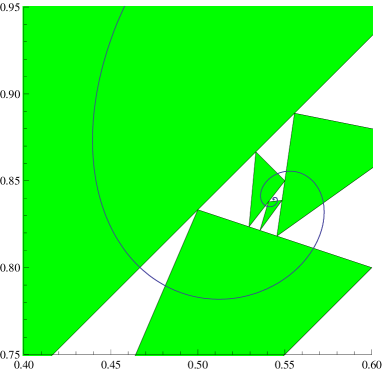
Figure 7: Detail, in the $z=1$ projective chart, of the first few zones of the Tribonacci sequence of stability zones starting by ${\cal D}_{(1:0:0)}$, ${\cal D}_{(0:1:0)}$ and ${\cal D}_{(0:0:1)}$. The labels of the zones shown above are, in decreasing area order, $(1:2:2)$, $(2:3:4)$, $(4:6:7)$, $(7:11:13)$ and $(13:20:24)$. All centers of the zones of the sequence lie on the smooth “Tribonacci projective spiral” drawn above which is converging to $(\alpha^{2}-\alpha-1,\alpha-1)\simeq(.543,.839)$.

Proposition 7.

The limit of every such sequences belongs to ${\cal E}$. In particular $(\alpha^{2}-\alpha-1:\alpha-1:1)\in{\cal E}$, where $\alpha$ is the Tribonacci constant, namely the real solution of the Tribonacci equation $x^{3}-x^{2}-x-1=0$.

Proof.

All vertices of stability zones of ${\cal C}$ are 1-rational points of ${\mathbb{R}}\hbox{\rm P}^{2}$ and therefore points on the boundaries have irrationality degree not higher than 2. Now, consider the sequence starting from the three squares $a_{1}={\cal D}_{(1:0:0)}$, $a_{2}={\cal D}_{(0:1:0)}$, $a_{3}={\cal D}_{(0:0:1)}$, so that the first few next terms of the sequence will be $a_{4}={\cal D}_{(1:1:1)}$, $a_{5}={\cal D}_{(1:2:2)}$, $a_{6}={\cal D}_{(2:3:4)}$ and so on: a simple calculation show that the label of the $n$th stability zone of the sequence, modulo terms in $\beta^{n}$ and $\bar{\beta}^{n}$, will be

$$(\frac{\beta\bar{\beta}}{(\alpha-\beta)(\alpha-\bar{\beta})}\alpha^{n}:\frac{-\beta-\bar{\beta}}{(\alpha-\beta)(\alpha-\bar{\beta})}\alpha^{n}:\frac{1}{(\alpha-\beta)(\alpha-\bar{\beta})}\alpha^{n})$$

where $\alpha=(1+\sqrt[3]{19-3\sqrt{33}}+\sqrt[3]{19+3\sqrt{33}})/3\simeq 1.84$ is the Tribonacci constant and $\beta,\bar{\beta}$ the remaining two solutions of the Tribonacci equation $x^{3}-x^{2}-x-1=0$. Since $|\beta|<\alpha$ the sequence of labels converges to the triple of coefficients of $\alpha^{n}$, namely $\ell_{\infty}=(\beta\bar{\beta}:-\beta-\bar{\beta}:1)=(\alpha^{2}-\alpha-1:\alpha-1:1)$; these three coordiantes are rationally independent so that $\ell_{\infty}$ has rationality degree $3$ and therefore it cannot belong to any boundary and for Proposition 4 it must belong to ${\cal E}$. ∎

Note that, since ${\cal E}$ is invariant by the $\psi_{a}$, this way we automatically get a countable number of explicit elements of ${\cal E}$.

Proposition 8.

Let $\{{\cal D}_{i}\}_{i\in\mathbb{N}}$ be the set of all stability zones sorted according to any recursive algorithm, e.g. ${\cal D}_{(i_{1}\dots i_{n})_{3}}=\psi_{i_{n}+1}\circ\dots\circ\psi_{i_{1}+1}({\cal D}_{(1:1:1)})$, where $(i_{1}\dots i_{n})_{3}$ is the base 3 expression for the index of the stability zone, and be $\ell_{n}$ the label associated to ${\cal D}_{n}$. Then $2\log_{3}^{2}(1+2n)+1\leqslant\|\ell_{n}\|^{2}\leqslant 3(1+2n)^{2\log_{3}\alpha}$ where $\alpha$ is the Tribonacci constant.

Proof.

A simple induction argument shows that, at every recursion level $k$, the biggest label belongs, modulo permutations of the projective coordinates, to the $k$th stability zone of the steepest descent sequence having as first three elements $D_{(0,0,1)}$, $D_{(0,1,0)}$ and $D_{(1,0,0)}$. Since at the $k$th recursion level there are $3^{k}$ stability zones it follows that $\|\ell_{\frac{3^{k}-1}{2}}\|\leqslant\sqrt{3}\alpha^{k}$ and therefore $\|\ell_{n}\|\leqslant\sqrt{3}(3n)^{\log_{3}\alpha}$.

The slowest sequence which can be formed by picking a stability zone for every recursion level is instead the one where ${\cal D}_{k}$ is the spawn of, say, $D_{(0,0,1)}$, $D_{(0,1,0)}$ and ${\cal D}_{k-1}$. In this case indeed $\|\ell_{\frac{3^{k}-1}{2}}\|=\sqrt{2(k+1)^{2}+1}$ from which follows immediately the left part of the inequality. ∎

Proposition 9.

Be ${\cal D}_{\ell}$ a stability zone with label $\ell$, $p_{\ell}$ its perimeter and $a_{\ell}$ its area in ${\mathbb{R}}\hbox{\rm P}^{2}$. Then there exist four constants $A$, $B$, $C$, $D$ such that

$$\frac{A}{\|\ell\|^{\frac{3}{2}}}\leqslant p_{\ell}\leqslant\frac{B}{\|\ell\|}\;,\;\;\frac{C}{\|\ell\|^{3}}\leqslant a_{\ell}\leqslant\frac{D}{\|\ell\|^{3}}$$

Proof.

The inequalities concerning $p_{\ell}$ are already known to be true in the general case.

To prove the ones relative to the area we change coordinates in ${\mathbb{R}}\hbox{\rm P}^{2}$ so that the three points $(1:0:1)$, $(0:1:1)$, $(1:1:0)$ become $(0:0:1)$, $(1:0:1)$, $(0:1:1)$. This way we can use the Lebesgue measure instead of the projective one and we can use the fact that $0\leqslant x,y\leqslant z$; now, be $(x_{i}:y_{i}:z_{i})$, $i=0,1,2$, the projective irreducible coordinates of the vertices $A_{i}$ of the triangle $T$ which encloses ${\cal D}_{\ell}$, so that $l=(\sum_{i}x_{i}:\sum_{i}y_{i}:\sum_{i}z_{i})$; the areas of $T$ and ${\cal D}_{\ell}$ are then easily computed respectively as ${\cal A}(T)=\Pi_{i=0}^{2}\frac{1}{z_{i}}$ and ${\cal A}({\cal D}_{\ell})=\Pi_{i=0}^{2}\frac{1}{z_{i}+z_{i+1}}$ (where the indices are meant modulo 3).

It is convenient for our purposes to consider the maximum norm $\|\ell\|_{\infty}$ since in the region under consideration $0\leqslant x,y\leqslant z$, so that we can assume without loss of generality that $x_{i},y_{i}\leqslant z_{i}$, $i=0,1,2$, and therefore we get trivially that

$${\cal A}({\cal D}_{\ell})=\frac{1}{(z_{0}+z_{1})(z_{1}+z_{2})(z_{2}+z_{0})}\geq\frac{1}{(z_{0}+z_{1}+z_{2})^{3}}=\frac{1}{\|\ell\|^{3}_{\infty}}$$

The second part of the inequality comes from the fact that if $\max z_{i}\leqslant\hbox{mid\ }z_{i}+\min z_{i}$ holds for the first triangle of the algoritm in Prop. 6 then it holds for every other triangle generated by the algorithm. Indeed assume to fix the ideas that $z_{0}\leqslant z_{1}\leqslant z_{2}$; then the new $z$ coordinates of the three vertices under the transform $\psi_{0}(z_{0}:z_{1}:z_{2})=(z_{0}:z_{1}+z_{0}:z_{2}+z_{0})$ satisfiy trivially again the relation $z^{\prime}_{2}\leqslant z^{\prime}_{0}+z^{\prime}_{1}$, and the very same happens for the tranforms under $\psi_{1}$. In case of $\psi_{2}$ we have $\{z^{\prime}_{0}=z_{0}+z_{2},z^{\prime}_{1}=z_{1}+z_{2},z^{\prime}_{2}=z_{2}\}$ so that the new larger $z$ is now $z^{\prime}_{1}$ but again $z^{\prime}_{1}\leqslant z^{\prime}_{2}+z^{\prime}_{0}$. Then finally

$$\frac{\|\ell\|^{3}_{\infty}}{(z_{0}+z_{1})(z_{1}+z_{2})(z_{2}+z_{0})}=\Bigl{(}1+\frac{z_{0}}{z_{1}+z_{2}}\Bigr{)}\Bigl{(}1+\frac{z_{1}}{z_{2}+z_{0}}\Bigr{)}\Bigl{(}1+\frac{z_{2}}{z_{0}+z_{1}}\Bigr{)}\leqslant 8$$

so that ${\cal A}({\cal D}_{\ell})\leqslant 8/\|\ell\|^{3}_{\infty}$. The final statement now follows from the fact that all norms are equivalent in finite dimension. ∎

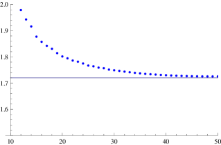
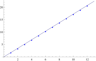
Figure 8: (a) Plot of $d_{n}=2-\log_{1.2}V({\cal E}_{1.2^{-n}})$ against $n$, where $V({\cal E}_{1.2^{-n}})$ is the volume of the neighborhood of ${\cal E}$ of radius $1.2^{-n}$; for “well-behaving” fractals this sequence converges to their Minkowsky dimension. The horizontal line shown in the picture has height $1.72$. (b) Plot of $\log_{2}N_{n}$ against $n$, where $N_{n}$ is the number of squares of side $2^{-n}$ which are not completely inside one of the 797161 stability zones found at the 12th recursion level. The angular coefficient of the straight line fitting the data in the picture is again $1.72$.

We could not find any way to evaluate exact non-trivial bounds for the fractal dimension of ${\cal E}$ but numerical calculations suggest that the dimension be smaller than 1.8.

A simple way to evaluate numerically fratal dimensions is using the Minkowsky dimension, namely the limit

$$\dim_{M}{\cal E}=2-\lim_{\epsilon\to 0}\frac{\log V({\cal E}_{\epsilon})}{\log\epsilon}$$

where $V({\cal E}_{\epsilon})$ is the surface of the $\epsilon$ neighborhood of ${\cal E}$. In order to do that we use the fact that, if $A$ is the area of $\Delta$ and $p$ its perimeter, then

$$V({\cal E}_{\epsilon})=p\epsilon+\epsilon\sum_{i=1}^{k_{\epsilon}}p_{i}+A-\sum_{i=1}^{k_{\epsilon}}a_{i}+\epsilon^{2}(\pi-\sum_{i=1}^{k_{\epsilon}}\frac{p_{i}^{2}}{4a_{i}})$$

where $k_{\epsilon}$ is the integer such that $\rho_{k_{\epsilon}+1}\leqslant\epsilon\leqslant\rho_{k_{\epsilon}}$ and $\rho_{k}$ is the radius of the inscribed circle to the triangle ${\cal D}_{k}$. In order to avoid infinities we make a projective change of coordinates so that the triangle $\Delta$ has vertices in $(0:0:1)$, $(1:0:1)$ and $(0:1:1)$. In Figure 8(a) we show the numerical results we got by evaluating the volume of the neighborhoods of ${\cal E}$ of radii $r_{n}=1.2^{-n}$ for $n=1,\ldots,50$, which suggests a fractal dimension between $1.7$ and $1.8$.

A second simple way is to evaluate an upper bound for the box-counting dimension, namely the limit

$$\dim_{B}{\cal E}=\lim_{\epsilon\to 0}\frac{\log N_{\epsilon}({\cal E})}{-\log\epsilon}$$

where $N_{\epsilon}({\cal E})$ is the smallest number of squares of side $\epsilon$ needed to cover ${\cal E}$ (even in this case we make the same change of coordinates to avoid infinities). In Figure 8(b) we show the results relative to covering with squares of side $2^{-n}$, $n=1,\cdots,12$, the complement of the 797161 triangles obtained by applying 12 times the recursion algorithm. Again we get a clear indication of the fractal dimension to be between 1.7 and 1.8.

4 Numerical generation of stability zones

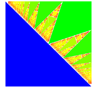
Figure 9: (a) Picture of the fractal in the square $[0,1]^{2}$ in the $z=1$ chart of ${\mathbb{R}}\hbox{\rm P}^{2}$ obtained by evaluating the soul of every stability zone in the lattice $(n,m,N)$, $n,m=1,\ldots,10^{3}$, $N=10^{3}$; (b) the same picture compared with the analytical boundaries of the $797161$ stability zones of the first $12$ levels of recursion. Out of the 961367 rational directions for which a label was numerically found by the algorithm, 455654 belong to those $797161$ stability zones and all of them turn out to lie within the analytical boundaries of the corresponding zone.

As an important byproduct of the study of stability zones of ${\cal C}$, we were able for the first time to compare very accurately the results of the NTC code [DeL99], used in [DeL03, DeL04, DeL06] to generate approximations of surfaces’ generality stability zones against their analytical boundaries.

Indeed no simple algorithm to generate the analytical equations of the boundaries of stability zones for a generic function is known so far but we know that all directions belonging to the same stability zone share the same soul and therefore it is possible to get an approximate picture of the set of generalized stability zones by evaluating the soul of some (big) set of rational directions. For example in all cases examined so far, thanks to the high level of symmetry, we could limit our analysis to the directions contained in the the triangle with sides $(0:0:1)$, $(1:1:1)$ and $(1:0:1)$ (concretely, to all directions $(m:n:N)$, $0<n<m<N$, for $N=10^{2},10^{3},10^{4}$).

Note that rational directions in this setting are of paramount importance because their (non-critical) leaves are compact (in ${\mathbb{T}}^{3}$) and therefore can be in principle approximated with error as small as wished and therefore the corresponding soul can be, at will, evaluated exactly through numerical calculations. Moreover, rational directions are dense in every stability zone and therefore (in principle) we do not lose any picture detail by restricting our analysis to them.

Below we present the algorithm we use to retrieve the soul (if any) of a rational direction $(m:n:N)$ in this particular case, where we have all saddles of “monkey” type:

• choose a representative $b_{i}$, $i=1,2,3$, for the cycles on ${\cal C}$ which are respectively homologous in ${\mathbb{T}}^{3}$ to the $x$, $y$ and $z$ axes;

• retrieve the intersection between ${\cal C}$ and the plane

  $$m(x-1/4)+n(y-1/4)+N(z-1/4)=0\,;$$

• follow the three critical loops and, if no saddle connection is detected, store them in the variables $c_{1,2,3}$, otherwise exit;

• evaluate the homology class of $c_{1,2,3}$ in ${\mathbb{T}}^{3}$;

• if exactly one of the three loops is non-zero in ${\mathbb{T}}^{3}$ then evaluate its intersection numbers with the $\{b_{i}\}$ and set this triple as the soul corresponding to the direction $(m,n,N)$, otherwise exit.

The result of sampling the triangle ${\cal T}$ with a $10^{3}\times 10^{3}$ lattice are shown in Figure 9 and turn out to be in perfect agreement with the analytical boundaries. An evaluation of the fractal box dimension based on these numerical data leads to a value of about $1.7$, which is also in very good agreement with the evaluation obtained from of the analytical boundaries made in sec. 3.2.

5 Acknowledgments

The authors gladly thanks the IPST (www.ipst.umd.edu) and the Dept. of Mathematics of the UMD (USA) (www.math.umd.edu) for their hospitality in the Spring Semester 2007 and for financial support. Numerical calculation were made on Linux PCs kindly provided by the UMD Mathematics Dept. and by the Cagliari section of INFN (www.ca.infn.it) which also provided financial support tho the first author. The authors also warmly thank S.P. Novikov and B. Hunt for several fruitful discussion during their stay at UMD.

References

- [CGS03] J. M. Sullivan C. Goodman-Strauss. Cubic polyhedra. Discrete Geometry: In Honor of W. Kuperberg’s 60th Birthday Monographs and Textbooks in Pure and Applied Mathematics, 253:305–330, 2003.
- [Cox37] H.S.M. Coxeter. Regular skew polyhedra in three and four dimensions. Proc. London Math. Soc., 43:33–62, 1937.
- [DeL99] R. DeLeo. Ntc library, http://ntc.sf.net/, 1999.
- [DeL03] R. DeLeo. Numerical analysis of the novikov problem of a normal metal in a strong magnetic field. SIADS, 2:4:517–545, 2003.
- [DeL04] R. DeLeo. Characterization of the set of “ergodic directions” in the novikov problem of quasi-electrons orbits in normal metals. RMS, 58(5):1042–1043, 2004.
- [DeL05] R. DeLeo. Proof of a dynnikov conjecture on the novikov problem of plane sections of periodic surfaces. RMS, 60(3):566–567, 2005.
- [DeL06] R. DeLeo. Topology of plane sections of periodic polyhedra with an application to the truncated octahedron. Experimental Mathematics, 15:109–124, 2006.
- [Dyn97] I.A. Dynnikov. Semiclassical motion of the electron. a proof of the novikov conjecture in general position and counterexamples. AMS Transl, 179:45–73, 1997.
- [Dyn99] I.A. Dynnikov. The geometry of stability regions in novikov’s problem on the semiclassical motion of an electron. RMS, 54:1:21–60, 1999.
- [NM03] S.P. Novikov and A.Ya. Maltsev. Dynamical systems, topology and conductivity in normal metals. J. of Statistical Physics, 115:31–46, 2003. cond-mat/0312708.
- [Nov82] S.P. Novikov. Hamiltonian formalism and a multivalued analog of morse theory. Usp. Mat. Nauk (RMS), 37:5:3–49, 1982.
- [Zor84] A.V. Zorich. A problem of novikov on the semiclassical motion of electrons in a uniform almost rational magnetic field. Usp. Mat. Nauk (RMS), 39:5:235–236, 1984.