Diagrammatic theory for Anderson Impurity Model.
Stationary property of the thermodynamic potential

Abstract

A diagrammatic theory around atomic limit is proposed for normal state of Anderson Impurity Model. The new diagram method is based on the ordinary Wick’s theorem for conduction electrons and a generalized Wick’s theorem for strongly correlated impurity electrons. This last theorem coincides with the definition of Kubo cumulants. For the mean value of the evolution operator a linked cluster theorem is proved and a Dyson’s type equations for one-particle propagators are established. The main element of these equations is the correlation function which contains the spin, charge and pairing fluctuations of the system. The thermodynamic potential of the system is expressed through one-particle renormalized Green’s functions and the correlation function. The stationary property of the thermodynamic potential is established with respect to the changes of correlation function.

I Introduction

The study of strongly correlated electron systems has become in the last decade one of the most active fields of condensed matter physics. One of the most important models of strongly correlated electrons is the Anderson impurity model (AIM)^[1]. It is a model of the system of free conduction electrons that interact with the system of the electrons of the $d-$ or $f-$ shells of impurity atoms. The impurity electrons are strongly correlated because of strong Coulomb repulsion and they undergo the hybridization with conduction electrons. This model has been largely applied to heavy fermion systems where the local impurity orbital is $f-$ orbital ^[2].

The interest towards the Anderson impurity model has also increased with the advent of Dynamical Mean Field Theory (DMFT) within which an infinite dimensional lattice models can be mapped onto effective impurity models by using self-consistency conditions^[3,4]. This model has also been intensively investigated by using the method of equation of motion for retarded and advanced Green’s functions proposed by Bogoliubov and Tiablikov ^[5] and developed in papers ^[6,7].

We propose a diagrammatic method to treat the AIM which is an alternative approach to the equations of motion and renormalization methods^[8,9]. The first attempt to develop the diagrammatic theory for this problem was realized in the paper^[10]. These authors used the expansion by cumulants for averages of products of Hubbard transfer operators and their algebra. Afterwards, other diagrammatic techniques dealing with perturbation in the hybridization amplitude while keeping the on-site correlation exact have been developed^[11-13]. Here we use the thermodynamic perturbation theory and Matsubara ^[14,15] Green’s functions, considering the hybridization of both groups of electrons as a perturbation.

The Hamiltonian of the model is written as

$$H = H_{0}+H_{int},$$

$$H_{0} = H_{0}^{c}+H_{0}^{f},$$

$$H_{0}^{c} = \sum\limits_{\mathbf{k}\sigma}\epsilon(\mathbf{k})\ C_{\mathbf{k}\sigma}^{+}C_{\mathbf{k}\sigma},$$

$$H_{0}^{f} = \epsilon_{f}\sum\limits_{\sigma}f_{\sigma}^{+}f_{\sigma}+Un_{\uparrow}^{f}n_{\downarrow}^{f},$$ (1)

$$H_{int} = \frac{1}{\sqrt{N}}\sum\limits_{\mathbf{k}\sigma}\left(V_{\mathbf{k}\sigma}f_{\sigma}^{+}C_{\mathbf{k}\sigma}+V_{\mathbf{k}\sigma}^{\ast}C_{\mathbf{k}\sigma}^{+}f_{\sigma}\right),$$

$$n_{\sigma}^{f} = f_{\sigma}^{+}f_{\sigma},$$

where $C_{\mathbf{k}\sigma}(C_{\mathbf{k}\sigma}^{+})$ and $f_{\sigma}(f_{\sigma}^{+})$ - annihilation (creation) operators of conduction and impurity electrons with spin $\sigma$ correspondingly, $\epsilon(\mathbf{k})$ is the kinetic energy of the conduction band state $(\mathbf{k},\sigma)$, $\epsilon_{f}\$ is the local energy of $f$ electrons, $U$ is the on-site Coulomb repulsion of the impurity electrons and $N$ the number of lattice sites. Both energies are evaluated with respect to the chemical potential $\mu$ of the system. The perturbation $H_{int}$ is the hybridization interaction between conduction and localized electrons. The Coulomb repulsion between impurity electrons is far to large to be treated as perturbation and it must be included in the main part of Hamiltonian $H_{0}$. The existence of this term invalidates the Wick theorem for local electrons. Therefore first of all we formulate the Generalized Wick theorem (GWT) for local electrons preserving the ordinary Wick theorem for conduction electrons. Our (GWT) really is the identity which determines the irreducible Green’s functions or the Kubo cumulants.

For example the chronological product of four local operators averaged with respect to zero-order density matrix of electrons has the form ^[16]:

$$\left\langle Tf_{1}f_{2}\overline{f}_{3}\overline{f}_{4}\right\rangle_{0} = \left\langle Tf_{1}\overline{f}_{4}\right\rangle_{0}\left\langle Tf_{2}\overline{f}_{3}\right\rangle_{0}-\left\langle Tf_{1}\overline{f}_{3}\right\rangle_{0}\left\langle Tf_{2}\overline{f}_{4}\right\rangle_{0}+g_{2}^{(0)ir}[1,2|3,4].$$ (2)

Here the symbol $\left\langle...\right\rangle_{0}$ means thermodynamical average on zero order distribution function. The right -hand part of equation (2) contains the first two terms which are the ordinary Wick contributions and last one named by us as irreducible Green’s function or Kubo cumulant which contains spin, charge and pairing fluctuations of localized electrons. In case when the statistical average of operators contains 6 operators $\left\langle Tf_{1}f_{2}f_{3}\overline{f}_{4}\overline{f}_{5}\overline{f}_{6}\right\rangle_{0}$, the right-hand part contains $3!$ terms with product of three one-particle Green’s functions, then there are nine terms in the form of product of one-particle Green’s function and two-particle irreducible function. At last there is a three-particle irreducible Green’s function $g_{3}^{(0)ir}[1,2,3|4,5,6]$. The Green’s functions $g_{n}^{(0)ir}[1,...,n\mid n+1,...,2n]$ which appear at the $n$-th order of the perturbation determine the structure of the new diagrammatic technique. Such definitions of irreducible Green’s functions has been used already for discussing the properties of the Hubbard and other strongly correlated models ^[17-21].

The zero order Hamiltonian of the localized electrons can be diagonalized by using the Hubbard transfer operators $\chi^{mn}$ ^[22]. By using these operators it is possible to calculate the simplest irreducible Green’s functions.

II Diagrammatical theory

The full one-particle Matsubara Green’s function of localized electrons in interaction representation has the form:

$$g_{\sigma\sigma^{\prime}}(\tau-\tau^{\prime}) = -\ \left\langle Tf_{\sigma}(\tau)\overline{f}_{\sigma^{\prime}}(\tau^{\prime})U(\beta)\right\rangle_{0}^{c},$$ (3)

where the index $c$ means connected diagrams. The operators are taken in the interaction representation , $T$ is chronological operator.

For conduction electrons it is convenient to define the local operator

$$b_{\sigma} = \frac{1}{\sqrt{N}}\sum\limits_{\mathbf{k}}V_{\mathbf{k}}C_{\mathbf{k}\sigma}.$$ (4)

The corresponding full conduction electron Green’s function has the form

$$G_{\sigma\sigma^{\prime}}(\tau-\tau^{\prime}) = -\ \left\langle Tb_{\sigma}(\tau)\overline{b}_{\sigma^{\prime}}(\tau^{\prime})U(\beta)\right\rangle_{0}^{c},$$ (5)

where $U(\beta)$ is the evolution operator

$$U(\beta) = T\exp(-\int\limits_{0}^{\beta}H_{int}(\tau)d\tau).$$ (6)

Because the matrix element of hybridization $V_{\mathbf{k}}$ is absorbed by local operator $b_{\sigma}$ it is convenient to introduce a new parameter $\lambda$, which will be associated to each vertex of the diagrams. In such a way the order of perturbation theory will be determined by $\lambda$ and not by the matrix element $V_{\mathbf{k}}$ of hybridization which can be present even in zero order Green’s function. In the last stage of the calculation $\lambda$ will be put equal to one.

In zero order of perturbation theory the Fourier representation of these functions are ($\overline{\sigma}=-\sigma$):

$$g_{\sigma\sigma^{\prime}}^{0}(i\omega) = \delta_{\sigma\sigma^{\prime}}g_{\sigma}^{0}(i\omega),$$

$$g_{\sigma}^{0}(i\omega) = \frac{1-n_{\overline{\sigma}}}{i\omega-\epsilon_{f}}+\frac{n_{\overline{\sigma}}}{i\omega-\epsilon_{f}-U},$$

$$n_{\overline{\sigma}} = \frac{\exp(-\beta\epsilon_{f})+\exp\left[-\beta(2\epsilon_{f}+U\right]}{Z_{0}},$$ (7)

$$Z_{0} = 1+2\exp(-\beta\epsilon_{f})+\exp\left[-\beta(2\epsilon_{f}+U\right].\$$

Here $\omega\equiv\omega_{n}=(2n+1)\pi/\beta$ are the Matsubara odd frequencies.

For the conduction electrons we have

$$G_{\sigma\sigma^{\prime}}^{0}(i\omega) = \delta_{\sigma\sigma^{\prime}}G_{\sigma}^{0}(i\omega),$$

$$G_{\sigma}^{0}(i\omega) = \frac{1}{N}\sum\limits_{\mathbf{k}}\frac{|V_{\mathbf{k}}|^{2}}{i\omega-\epsilon(\mathbf{k})}.$$ (8)

The presence in the definition of zero order Green’s function $G_{\sigma}^{0}$ of the square of matrix element of hybridization is the consequence of our equation (4) and not of the perturbation.

The thermodynamical perturbation theory gives us the results for one-particle Green’s functions presented on the Fig.1 and Fig.2. The double solid and dashed lines depict the renormalized and the thin lines the bar propagators of conduction and impurity electrons. The lines connect the crosses which depict the impurity states. To crosses are attached two arrows one of which is ingoing and one outgoing. They depict the annihilation and creation of the electrons correspondingly. The crosses are the vertices of the diagrams and a $\lambda$ multiplier is attached to each of them. The index $n$ means $(\sigma_{n},\tau_{n})$. The summation on the index $\sigma_{n}$ and the integration on the $\tau_{n}$ are intended. The rectangles with $2n$ indices and crosses depict the irreducible $g_{n}^{(0)ir}[1,...,n\mid n+1,...,2n]$ Green’s functions. The sign of diagrams is determined by the parity (even or odd) of the permutation of the Fermi operators necessary to obtain the diagram.

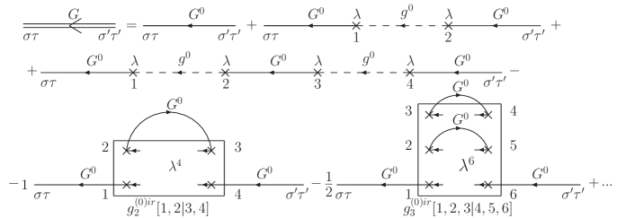
Figure 1: Diagrams of first orders of perturbation theory for the conduction electron propagator. The thin solid lines represent the conduction electron propagator and dashed lines the impurity electron propagator of zero order. Double line represents the full propagator.

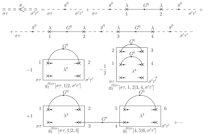
Figure 2: The diagrams for impurity electron propagator $g_{\sigma\sigma^{\prime}}(\tau-\tau^{\prime})$. The last three diagrams contain the correlation contributions. Two of them are strong connected and the last is weak connected.

Using Feynman’s rules and the correspondence above, it is possible to establish the next equation for the diagrams shown in Fig.1:

$$G_{\sigma\sigma^{\prime}}(\tau-\tau^{{}^{\prime}}|\lambda) = G_{\sigma\sigma^{\prime}}^{0}(\tau-\tau^{{}^{\prime}})+\sum\limits_{\sigma_{1}\sigma_{2}}\int\limits_{0}^{\beta}d\tau_{1}\int\limits_{0}^{\beta}d\tau_{2}G_{\sigma\sigma_{1}}^{0}(\tau-\tau_{1})\lambda g_{\sigma_{1}\sigma_{2}}(\tau_{1}-\tau_{2}|\lambda)\lambda G_{\sigma_{2}\sigma^{\prime}}^{0}(\tau_{2}-\tau^{{}^{\prime}}).$$ (9)

On the basis of the diagrams depicted on the Fig.2, instead it is possible to establish the following Dyson’s type equation for $g_{\sigma\sigma^{\prime}}$:

$$g_{\sigma\sigma^{\prime}}(\tau-\tau^{{}^{\prime}}|\lambda) = \Lambda_{\sigma\sigma^{\prime}}(\tau-\tau^{{}^{\prime}}|\lambda)+\sum\limits_{\sigma_{1}\sigma_{2}}\int\limits_{0}^{\beta}d\tau_{1}\int\limits_{0}^{\beta}d\tau_{2}\Lambda_{\sigma\sigma_{1}}(\tau-\tau_{1})\lambda G_{\sigma_{1}\sigma_{2}}^{0}(\tau_{1}-\tau_{2})\lambda g_{\sigma_{2}\sigma^{\prime}}(\tau_{2}-\tau^{{}^{\prime}}),$$ (10)

where

$$\Lambda_{\sigma\sigma^{\prime}}(\tau-\tau^{{}^{\prime}}|\lambda) = g_{\sigma\sigma^{\prime}}^{0}(\tau-\tau^{{}^{\prime}})+Z_{\sigma\sigma^{\prime}}(\tau-\tau^{{}^{\prime}}|\lambda).$$ (11)

Here $Z_{\sigma\sigma^{\prime}}$ is the new correlation function which contains an infinite sum of the irreducible Green’s functions. As it was underlined above this function contains all spin, charge and pairing fluctuations and is the main element of our diagram technique.

Diagram representation of the correlation function $\Lambda_{\sigma\sigma^{\prime}}(\tau-\tau^{{}^{\prime}}|\lambda)$ is depicted on the Fig.3

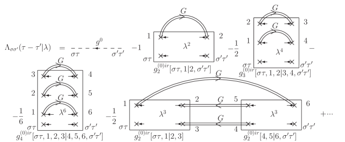
Figure 3: Diagram representation of the correlation function $\Lambda_{\sigma\sigma^{\prime}}$. Double solid lines depict the renormalized conduction electron propagators $G_{\sigma\sigma^{\prime}}(\tau-\tau^{{}^{\prime}}|\lambda)$. The arguments of irreducible functions are supposed arranged in the clock wise direction.

The series expansion of the full propagator $G_{\sigma\sigma^{\prime}}(\tau-\tau^{\prime})$ can gives us more detailed representation of this quantity.

By using the Fourier representation of Matsubara functions on the base of equations (9)and (10), we have:

$$G_{\sigma}(i\omega|\lambda)=\frac{G_{\sigma}^{0}(i\omega)}{1-\Lambda_{\sigma}(i\omega|\lambda)G_{\sigma}^{0}(i\omega)\lambda^{2}}.$$ (12)

$$g_{\sigma}(i\omega|\lambda)=\frac{\Lambda_{\sigma}(i\omega|\lambda)}{1-\Lambda_{\sigma}(i\omega|\lambda)G_{\sigma}^{0}(i\omega)\lambda^{2}}.$$ (13)

The equation (12) for conduction electron propagator is the Dyson one with mass operator determined by the correlation function of impurity electrons:

$$\Sigma_{\sigma}(i\omega|\lambda)=\lambda^{2}\Lambda_{\sigma}(i\omega|\lambda).$$ (14)

When $\lambda$ is equal to one these quantities coincide.

The equation (13) for impurity electrons is of Dyson type and coincides, for $\lambda=1$, with other equations obtained for strongly correlated electrons ^[17-21]. In equations (12), (13) the parameter $\lambda$ can be taken equal to one and can be omitted.

III Thermodynamic Potential

The thermodynamic potential of our strongly correlated system is equal to

$$F = F_{0}-\frac{1}{\beta}\ln\left\langle U(\beta)\right\rangle_{0},$$

$$F_{0} = -\frac{1}{\beta}\ln Z_{0}-\frac{2}{\beta}\sum\limits_{\mathbf{k}}\ln\left[1+\exp(-\beta\epsilon(\mathbf{k)})\right],$$

The diagrams which determine the mean value of the evolution operator $\left\langle U(\beta)\right\rangle_{0}$ have not external lines and are named vacuum diagrams. Between such diagrams there are connected and disconnected ones. The disconnected diagrams can be summed and the result of such summation is equal to the exponent of connected diagrams. The result of such summation permits us to formulate linked cluster theorem. It has the form:

$$\left\langle U(\beta)\right\rangle_{0}=\exp\left\langle U(\beta)\right\rangle_{0}^{c},$$ (16)

where $\left\langle U(\beta)\right\rangle_{0}^{c}$ is the infinite sum of vacuum connected diagrams. This quantity is equal to zero when hybridization is absent.

Therefore thermodynamic potential is equal to

$$F=F_{0}-\frac{1}{\beta}\left\langle U(\beta)\right\rangle_{0}^{c},$$ (17)

In Fig.4 are depicted some of the simplest vacuum diagrams.

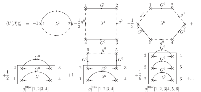
Figure 4: Connected vacuum diagrams of the second, fourth and sixth order of perturbation theory.

The first three diagrams are of chain type and are originated from the ordinary Wick contributions. The last three diagrams contain the correlation functions and are determined by the new contributions of GWT. The factor $\frac{1}{n}$, where $n$ is the perturbation theory order, present in these diagrams makes it difficult to carry out the summation over $n$. As is usual in such cases ^[23] we employ a trick, that of integrating over the interacting strength $\lambda$. The result of this procedure is depicted in Fig.5.

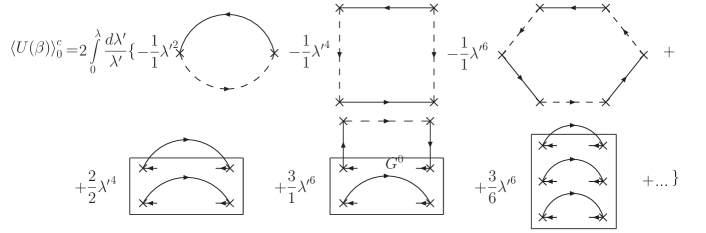
Figure 5: The result of integration over the interacting strength of the vacuum diagrams.

Now we shall use the diagrams of the conduction electron propagator $G_{\sigma}$ depicted on the Fig.1 and these of $\Lambda_{\sigma}$ from Fig.3 to combine them in such a way to obtain the vacuum diagrams of Fig.5. Either diagrams of Fig.5 of the $n$ order of perturbation theory can be considered as the product of the contribution of order $n_{1}$ from $G_{\sigma}$ and of the contribution of order $n_{2}$ from $\Lambda_{\sigma}$ with the condition that $n_{1}+n_{2}=n$. There are in general case different possibilities to arrange such contribution and the number of these possibilities is determined by the numerator of the fraction before the diagrams of Fig.5. The denominator of this fraction is determined from Fig.4. Therefore we obtain

$$\left\langle U(\beta)\right\rangle_{0}^{c}=(-2)\sum\limits_{\sigma_{1}\sigma_{2}}\int\limits_{0}^{\beta}d\tau_{1}\int\limits_{0}^{\beta}d\tau_{2}\int\limits_{0}^{\lambda}\frac{d\lambda^{\prime}}{\lambda^{\prime}}G_{\sigma_{1}\sigma_{2}}(\tau_{1}-\tau_{2}|\lambda^{\prime})\Sigma_{\sigma_{2}\sigma_{1}}(\tau_{2}-\tau_{1}|\lambda^{\prime})=$$ (18)

$$=(-2)\sum\limits_{\sigma}\sum\limits_{\omega}\int\limits_{0}^{\lambda}\frac{d\lambda^{\prime}}{\lambda^{\prime}}G_{\sigma}(i\omega|\lambda^{\prime})\Sigma_{\sigma}(i\omega|\lambda^{\prime}).$$

The thermodynamical potential becomes equal to

$$F=F_{0}+\frac{2}{\beta}\sum\limits_{\sigma}\sum\limits_{\omega}\int\limits_{0}^{\lambda}\frac{d\lambda^{\prime}}{\lambda^{\prime}}G_{\sigma}(i\omega|\lambda^{\prime})\Sigma_{\sigma}(i\omega|\lambda^{\prime}).$$ (19)

From this equation we obtain:

$$\lambda\frac{\partial F}{\partial\lambda}=\frac{2}{\beta}\sum\limits_{\sigma}\sum\limits_{\omega}G_{\sigma}(i\omega|\lambda)\Sigma_{\sigma}(i\omega|\lambda).$$ (20)

The expression (19) for thermodynamical potential contains additional integration over the interaction strength $\lambda$ and is awkward because of it. As was proved for non correlated many-electron system by Luttinger and Ward ^[23] this expression can be transformed into a much more convenient formula.

We consider the following expression:

$$Y=-\frac{1}{\beta}\sum\limits_{\sigma}\sum\limits_{\omega}\exp(i\omega 0^{+})\{\ln[G_{\sigma}^{0}(i\omega)\Sigma_{\sigma}(i\omega|\lambda)-1]+G_{\sigma}(i\omega|\lambda)\Sigma_{\sigma}(i\omega|\lambda)\}+Y^{\prime},$$ (21)

which is the generalization of the Luttinger-Ward equation for strongly correlated systems. Here $Y^{\prime}$ is the sum of closed linked skeleton diagrams with full $G_{\sigma}$ function as a contribution of conduction electron lines.

On the Fig.6 are depicted some of simplest skeleton diagrams.

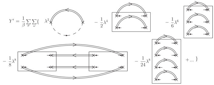
Figure 6: Closed linked skeleton diagrams. The double solid lines correspond to full propagators $G_{\sigma}(i\omega|\lambda)$ of conduction electrons. The rectangles correspond to the correlation functions of the correlated electrons.

These diagrams depend on the interaction strength $\lambda$ not only through the factors in front of each diagram but also through the full Green’s function $G_{\sigma}(i\omega|\lambda)$.

From equations (12), (14) and (21) we obtain

$$\frac{\partial Y}{\partial\Sigma_{\sigma}(i\omega|\lambda)} = -\frac{1}{\beta}\Sigma_{\sigma}(i\omega|\lambda)\ G_{\sigma}^{2}(i\omega|\lambda)+$$

$$+\frac{\partial Y^{\prime}}{\partial\Sigma_{\sigma}(i\omega|\lambda)},$$ (22)

where, from Fig.3,6 and definition (14), it follows that

$$\frac{\partial Y^{\prime}}{\partial G_{\sigma}(i\omega|\lambda)}=\frac{\lambda^{2}}{\beta}\Lambda_{\sigma}(i\omega|\lambda)=\frac{\Sigma_{\sigma}(i\omega|\lambda)}{\beta}.$$ (23)

As a result we obtain the stationary property with respect to changes of the mass operator:

$$\frac{\partial Y}{\partial\Sigma_{\sigma}(i\omega|\lambda)}=0.$$ (24)

Now we shall find the quantity $\frac{\partial Y}{\partial\lambda}$ . By the stationary property of $Y$ we can ignore the dependence of $\Sigma_{\sigma}$ and $G_{\sigma}$ on $\lambda$ and take into account only the explicit dependence of $\lambda$ in $Y^{\prime}$, depicted on the Fig.6. From this figure it is easy to obtain:

$$\lambda\frac{\partial Y}{\partial\lambda}\mid_{\Sigma}=\lambda\frac{\partial Y^{\prime}}{\partial\lambda}\mid_{\Sigma}=\frac{2}{\beta}\sum\limits_{\sigma}\sum\limits_{\omega}G_{\sigma}(i\omega|\lambda)\Sigma_{\sigma}(i\omega|\lambda).$$ (25)

From equations (20) and (25) we obtain

$$\lambda\frac{\partial F}{\partial\lambda}=\lambda\frac{\partial Y}{\partial\lambda}.$$ (26)

The consequence of this equation is the solution

$$F(\lambda)=Y(\lambda)+\textsc{const}.$$ (27)

For $\lambda=0$ we have $Y(0)=0$ and $F(o)=F_{0}$. Therefore $\textsc{const}=F_{0}$.

The final result has the form

$$F=F_{0}+Y.$$ (28)

IV Conclusions

The thermodynamic potential of a strongly correlated system described by the Anderson impurity model has been calculated. We have formulated a new diagrammatic technique for fermions with strong correlations and determined the correlation function of localized electrons and mass operator of conduction electrons. For the conduction electrons this operator coincides with the correlation function of the impurity electrons. A Dyson’s type of equation for the one-particle propagators of both subsystems, of conduction and impurity electrons, has been established. Within our diagrammatic technique we first obtained an exact expression for the thermodynamic potential as a product of the full propagator $G_{\sigma}$ of the conduction electrons and its mass operator $\Sigma_{\sigma}$, then a Luttinger-Ward-type ^[23] of identity based on the stationary property of the potential was established. The expression for the thermodynamic potential so obtained could be very useful to calculate in a systematic way all thermodynamic quantities (e.g. specific heat) of strongly correlated electron systems.