Hydrostatic gas distributions: global estimates of temperature and abundance

Abstract

Estimating the temperature and metal abundance of the intracluster and the intragroup media is crucial to determine their global metal content and to determine fundamental cosmological parameters. When a spatially resolved temperature or abundance profile cannot be recovered from observations (e.g., for distant objects), or deprojection is difficult (e.g., due to a significant non-spherical shape), only global average temperature and abundance are derived. After introducing a general technique to build hydrostatic gaseous distributions of prescribed density profile in potential wells of any shape, we compute the global mass weighted and emission weighted temperature and abundance for a large set of barotropic equilibria and an observationally motivated abundance gradient. We also compute the spectroscopic-like temperature that is recovered from a single temperature fit of observed spectra. The derived emission weighted abundance and temperatures are higher by 50% to 100% than the corresponding mass weighted quantities, with overestimates that increase with the gas mean temperature. Spectroscopic temperatures are intermediate between mass and luminosity weighted temperatures. Dark matter flattening does not lead to significant differences in the values of the average temperatures or abundances with respect to the corresponding spherical case (except for extreme cases).

1 Introduction

The amount of metals in the Intracluster Medium (ICM) and in the Intragroup Medium (IGM) gives us important clues about the past star formation activity of the stellar population of these galaxy systems, being it directly linked to the total number of supernovae exploded in the past and to the initial stellar mass function of the star formation epoch (e.g., Renzini et al. 1993). The metal content can also enlight how the enrichment proceeded, e.g., via stripping or galactic winds driven by SNe or AGN feedback, and has implications for both the ICM/IGM and galaxy evolution (e.g., Wu, Fabian, & Nulsen 2000; Finoguenov et al. 2001; Kapferer et al. 2007). For these reasons the observational study of the metal content of the ICM/IGM is growing fastly. After the first large compilation of (emission weighted) average abundance values of iron from $EXOSAT$, $Einstein$ and $GINGA$ observations (Arnaud et al. 1992), $ASCA$ made metal measurements for many clusters (Fukazawa et al. 1994, Finoguenov et al. 2000, Baumgartner et al. 2005). The average iron abundance was estimated to be $0.38\pm 0.07$ and $0.21\pm 0.05$ respectively for the cooling flow and non cooling flow clusters (Allen & Fabian 1998). In more recent times, the superior quality of the $XMM-Newton$ and $Chandra$ instrumentation has allowed for more accurate determinations of the elemental abundance pattern (e.g., Tamura et al. 2004, Fukazawa et al. 2004, Durret et al. 2005, Sanders & Fabian 2006, de Plaa et al. 2007, Finoguenov et al. 2007, Rasmussen & Ponman 2007). Nowadays, these studies are carried on also with $Suzaku$ (e.g., Matsushita et al. 2007, Sato et al. 2007).

Similarly to the metal abundance, the hot ICM/IGM temperature is also one of the most important and commonly used global observables: it is used as a proxy for the total mass of the system (e.g., Voit 2005), from which the clusters can be used as probes for fundamental cosmological parameters (e.g., Henry & Arnaud 1991, Henry 1997, Nevalainen et al. 2000, Arnaud et al. 2005). Temperature profiles have been built with improved quality in the recent past (e.g., Arnaud et al. 2005, Pointecouteau et al. 2005, Vikhlinin et al. 2005, 2006, Pratt et al. 2007, Rasmussen & Ponman 2007). Since the ICM/IGM are not isothermal, ideally the mass weighted temperature should enter the computation of quantities to be used for cosmological tests.

From a more quantitative point of view, the amount of the mass of metals in the ICM/IGM is given by

$$M_{\rm gas}^{Z}=\int\rho({\bf x})Z({\bf x})d^{3}{\bf x},$$ (1)

where $\rho$ and $Z$ are the true three dimensional gas density and abundance profiles. Thus, the mass weighted average abundance is given by

$$<Z>={M_{\rm gas}^{Z}\over M_{\rm gas}},$$ (2)

where $M_{\rm gas}=\int\rho({\bf x})d^{3}{\bf x}$ is the total hot gas mass. Similarly, the mass weighted average temperature is

$$<T>={\int\rho({\bf x})T({\bf x})d^{3}{\bf x}\over M_{\rm gas}}.$$ (3)

Unfortunately, there are at least three serious problems with estimating $<Z>$ and $<T>$ from observations: 1) for many clusters/groups we do not know the intrinsic shape of the gas distribution and the viewing angles under which we are observing it; therefore, one cannot uniquely deproject observed quantities (obtained in general from X-ray data) to derive $\rho$, $T$, and $Z$; 2) even for spherically symmetric systems, deprojection is a demanding numerical process, very sensitive to the properties of the instrumental PSF and to measurement errors (e.g., Finoguenov & Ponman 1999); 3) in many cases only a single spectrum can be extracted for the whole gas, and only an average abundance and temperature can be obtained; this happens when there are not enough counts for a spatially resolved spectroscopy, e.g., for distant clusters/groups (Hashimoto et al. 2004, Maughan et al. 2007, Baldi et al. 2007 for recent observations with Chandra and XMM-$Newton$). In particular, the average abundance and temperature mentioned in point 3) above are not those given in eqs. (2)-(3), but are in practice luminosity weighted quantities (e.g., Mathiesen & Evrard 2001, Mazzotta et al. 2004, Maughan et al. 2007, Rasia et al. 2005, Kapferer et al. 2007) that can be defined as

$$<Z>_{L}={\displaystyle{\int\Sigma_{\rm X}(\xi_{1},\xi_{2})Z_{\rm pr}(\xi_{1},\xi_{2})d\xi_{1}d\xi_{2}\over L_{\rm X}}},$$ (4)

and

$$<T>_{L}={\displaystyle{\int\Sigma_{\rm X}(\xi_{1},\xi_{2})T_{\rm pr}(\xi_{1},\xi_{2})d\xi_{1}d\xi_{2}\over L_{\rm X}}},$$ (5)

where $(\xi_{1},\xi_{2})$ are the coordinates of the projection plane, $\Sigma_{\rm X}$ is the X-ray ICM surface brigthness, $Z_{\rm pr}$ and $T_{\rm pr}$ are the luminosity weighted projected abundance and temperature, and $L_{\rm X}=\int\Sigma_{\rm X}d\xi_{1}d\xi_{2}$ is the total X-ray luminosity (see Appendix A1).

It is then natural to investigate the relation between the quantities in eqs. (2)-(3) and (4)-(5). For example, Rasia et al. (2008), using mock $XMM-Newton$ spectra for a sample of simulated clusters, find that the iron abundance inferred from such spectra is very close to the projection of the emission weighted values of $Z$ (i.e., $<Z>_{L}$), at least for thermal components of $kT>3$ keV and $kT<2$ keV. Kapferer et al. (2007), again using simulations, similarly find that for $kT>3$ keV the X-ray emission weighted abundance is close within few percents to that derived from the analysis of synthetic X-ray spectra. Unfortunately, neglecting a possible spatial variation of the metal abundance can lead to largely wrong estimates of $M_{\rm gas}^{Z}$ when using $<Z>_{L}$ instead of $<Z>$ in eq. (2) (Arnaud et al. 1992). In fact, iron distributions peaked towards the cluster/group center have been revealed in many cases (Fukazawa et al. 2000, Ettori et al. 2002, Sanders & Fabian 2002, Matsushita et al. 2003, Böhringer et al. 2004, Tamura et al. 2004). Motivated by this, in an exploratory study Pellegrini & Ciotti (2002) showed that in these cases $<Z>$ can be significantly smaller than $<Z>_{L}$. Successively, De Grandi et al. (2004) confirmed this result for their sample of cooling core clusters, for which they estimated $<Z>$ to be $\sim 15$% smaller than $<Z>_{L}$.

It is also well accepted that the ICM/IGM have a temperature structure that was established by gravitational and non-gravitational processes, as radiative cooling and heating by active galactic nuclei (see Borgani et al. 2005, Vikhlinin et al. 2005, Piffaretti et al. 2005, Arnaud et al. 2005, Donahue et al. 2006). Efforts have been made recently to understand the meaning of the temperature derived from spectroscopic observations when the ICM/IGM has a complex thermal structure (Mazzotta et al. 2004, Rasia et al. 2005, Vikhlinin 2006, Nagai et al. 2007). Mazzotta et al. (2004) found that the observed temperature, recovered from a single temperature fit to the spectrum of a plasma with components at different temperatures (but all continuum-dominated, i.e., with $kT{\mathrel{\mathchoice{\lower 2.9pt\vbox{\halign{$\m@th\displaystyle\hfil#\hfil$\cr>\crcr\sim\crcr}}}{\lower 2.9pt\vbox{\halign{$\m@th\textstyle\hfil#\hfil$\cr>\crcr\sim\crcr}}}{\lower 2.9pt\vbox{\halign{$\m@th\scriptstyle\hfil#\hfil$\cr>\crcr\sim\crcr}}}{\lower 2.9pt\vbox{\halign{$\m@th\scriptscriptstyle\hfil#\hfil$\cr>\crcr\sim\crcr}}}}}3$ keV) and extracted from $Chandra$ or $XMM-$Newton data, is well approximated by a ”spectroscopic-like temperature” $T_{\rm sl}$ (see Sect. 3). Vikhlinin (2006) extended this previous work and proposed an algorithm to accurately predict $T_{\rm sl}$ that would be derived for a plasma with components in a wider range of temperatures ($kT{\mathrel{\mathchoice{\lower 2.9pt\vbox{\halign{$\m@th\displaystyle\hfil#\hfil$\cr>\crcr\sim\crcr}}}{\lower 2.9pt\vbox{\halign{$\m@th\textstyle\hfil#\hfil$\cr>\crcr\sim\crcr}}}{\lower 2.9pt\vbox{\halign{$\m@th\scriptstyle\hfil#\hfil$\cr>\crcr\sim\crcr}}}{\lower 2.9pt\vbox{\halign{$\m@th\scriptscriptstyle\hfil#\hfil$\cr>\crcr\sim\crcr}}}}}0.5$ keV) and arbitrary abundances of heavy elements. From the analysis of mock spectra of simulated clusters, it was found that $T_{\rm sl}$ is lower than the emission weighted temperature $<T>_{L}$, with consequences for using the observed $M-T$ relation to infer the amplitude of the power spectrum of primordial fluctuations (Rasia et al. 2005).

Here, extending the preliminary discussion of Pellegrini & Ciotti (2002) based on spherical models, we estimate how much discrepant $<Z>_{L}$ and $<Z>$, and $<T>_{L}$ (or $T_{\rm sl}$) and $<T>$ are, by using different plausible profiles for $\rho$, $T$ and $Z$ obtained assuming hydrostatic equilibrium within triaxial mass distributions resembling real systems. In particular the models are constructed by using a technique that allows for building analytical barotropic gas distributions with prescribed density profiles departing from spherical symmetry. These new models extend the class of equilibria usually considered in the literature beyond isothermal or polytropic models (i.e., Suto, Sasaki & Makino 1998; Pellegrini & Ciotti 2002; Lee & Suto 2003, 2004; Ostriker, Bode & Babul 2005; Ascasibar & Diego 2007). In the computation of the averages, our approach takes also advantage of the Projection Theorem, from which it follows that $<Z>_{L}$ and $<T>_{L}$ are independent of the specific direction of the line-of-sight, and can be calculated using the intrinsic three-dimensional quantities of the models, with a much easier procedure that avoids projection and surface integration.

The paper is organized as follows. In Section 2 we present the models of the dark matter halos and the procedure to build fully analytical hydrostatic configurations in potentials of triaxial shape, for gas distributions corresponding to truncated quasi-isothermal models, quasi-polytropic models and modified $\beta$ models. In Section 3 we describe the results and in Section 4 we summarize the main conclusions; technical results are reported in the Appendix.

2 The models

2.1 Density profiles for the gravitating mass

The density of the (dark) mass distribution is the generalization to the triaxial case of the so-called $\gamma$-models (Dehnen 1993, Tremaine et al. 1994):

$$\varrho={M(3-\gamma)\over 4\pi r_{\rm c}^{3}(1-\epsilon)(1-\eta)}{1\over m^{\gamma}(1+m)^{4-\gamma}},$$ (6)

where

$$m^{2}={x^{2}\over r_{\rm c}^{2}}+{y^{2}\over(1-\epsilon)^{2}r_{\rm c}^{2}}+{z^{2}\over(1-\eta)^{2}r_{\rm c}^{2}},$$ (7)

$M$ is the total dark mass of the system, $r_{\rm c}$ is a characteristic scale, and the pair $(\epsilon,\eta)$ parameterizes the flattening along the $y$ and $z$ axes respectively. The mass distribution is spherically symmetric when $\epsilon=\eta=0$, and $M$ remains constant for different choices of the flattening. For simplicity, we restrict to the $\gamma=0$ and the $\gamma=1$ cases: in the former, the density profile shows a central “core”, while in the latter the Hernquist (1990) profile is recovered in the spherical limit. Note that the $\gamma=1$ models have the same radial trend, in the central regions, as the profile obtained from high resolution cosmological simulations (Dubinsky & Carlberg 1991; Navarro, Frenk & White 1996), while they are steeper at large radii ($\propto r^{-4}$ instead of $\propto r^{-3}$). Even though not required by the technique described in Sect. 2.2, in our analysis we used the potential profiles obtained by means of homeoidal expansions of the true potential at fixed total mass (e.g., Muccione & Ciotti 2003, 2004; Lee & Suto 2003, 2004; Ciotti & Bertin 2005, hereafter CB05). This approach has the advantage of avoiding the numerical integration needed to recover the potential (e.g. Binney & Tremaine 2008), and the formulae obtained are a very good approximation of the exact potential associated with eq. (6).

Figure 1: Radial profiles of density and temperature for truncated quasi-isothermal spherical gas models in the Hernquist potential (left, $r_{\rm t}=r_{\rm vir}=6r_{\rm c}$) and in the $\gamma=0$ potential (right, $r_{\rm t}=r_{\rm vir}=10r_{\rm c}$), with $T_{\rm vir}=2.3\,{\rm keV}$. Three values of $T_{0}$ of the parent isothermal model have been chosen: $T_{0}=0.8\,T_{\rm vir}$ (solid lines), $T_{0}=1.5\,T_{\rm vir}$ (dotted lines) and $T_{0}=3\,T_{\rm vir}$ (dashed lines). The distance from the center $r$ is normalized to $r_{200}$ as defined at the end of Sect. 2.1.

Homeoidal expansion applied to the $\gamma=0$ model shows that

$$\tilde{\phi}=-{2r+1\over 2(r+1)^{2}}-\left[{3r^{2}+12r+8\over 2(r+1)^{2}}-{4\ln(r+1)\over r}\right]{\epsilon+\eta\over r^{2}}-$$

$$\left[{12\ln(r+1)\over r}-{3r^{3}+22r^{2}+30r+12\over(r+1)^{3}}\right]{\epsilon y^{2}+\eta z^{2}\over r^{4}},\quad\quad$$ (8)

where $\phi=GM\tilde{\phi}/r_{\rm c}$, and the value of the central potential is $\tilde{\phi}_{0}=-(3+\epsilon+\eta)/6$. For the $\gamma=1$ model

$$\tilde{\phi}=-{1\over r+1}-\left[{r+2\over r+1}-{2\ln(r+1)\over r}\right]{\epsilon+\eta\over r^{2}}-$$

$$\left[{6\ln(r+1)\over r}-{2r^{2}+9r+6\over(r+1)^{2}}\right]{\epsilon y^{2}+\eta z^{2}\over r^{4}},$$ (9)

and $\tilde{\phi}_{0}=-(3+\epsilon+\eta)/3$. In the formulae above the radial coordinates are normalized to $r_{\rm c}$, and in both cases the expansion holds for $1\geq 3\eta-\epsilon$ (see Appendix A in CB05). Thus, in principle the maximum deviation from spherical symmetry is obtained for $\eta=\epsilon=0.5$, corresponding to a prolate system of axis ratio 2:1. Finally, the virial temperature of the system (defined as $3kMT_{\rm vir}\equiv|U|$, where $U$ is the gravitational energy) in the limit of small flattenings, and independently of the specific density profile $\varrho(m)$, is given by

$$T_{\rm vir}={GM\over 3r_{\rm vir}}{\mu m_{\rm H}\over k}\left(1+{\epsilon+\eta\over 3}\right),$$ (10)

where $\mu$ is the mean particle weight, $m_{\rm H}$ is the proton mass, $k$ is the Boltzmann constant and $r_{\rm vir}$ is the virial radius of $\varrho$ in the spherical limit (Muccione & Ciotti 2004). Here $r_{\rm vir}=10r_{\rm c}$ and $6r_{\rm c}$ for the $\gamma=0$ and $\gamma=1$ models, respectively. Note that, for fixed $M$ and $r_{\rm vir}$, $T_{\rm vir}$ increases for an increasing flattening.

Summarizing, the potential is determined by assigning the two flattenings $\epsilon$ and $\eta$, and by choosing the mass $M$, the slope $\gamma$, and $r_{\rm c}$. The latter step is done via the relation $r_{\rm vir}=r_{\rm vir}(M)$ holding for dark matter halos obtained from cosmological simulations in a flat $\Lambda$CDM cosmological model ($\Omega_{m}=0.3$, $\Omega_{\Lambda}=0.7$, $h=0.7$, where the Hubble constant is defined as $100h$ km s^-1 Mpc^-1), as derived, e.g., by Lanzoni et al. (2004). For example, for a mass $M=3.5\times 10^{14}h^{-1}M_{\odot}$ we adopt $r_{\rm vir}=1.4h^{-1}$ Mpc, so that $r_{\rm c}=0.14h^{-1}$ Mpc for the $\gamma=0$ model, and $r_{\rm c}=0.23h^{-1}$ Mpc for the Hernquist model, with $T_{\rm vir}=2.3$ keV (spherical case). For $M=1.0\times 10^{15}h^{-1}M_{\odot}$, $r_{\rm vir}=1.8h^{-1}$ Mpc and $T_{\rm vir}=5.1$ keV (spherical case). We also derived the commonly used $r_{200}$ and $r_{500}$ radii (within which the average mass density is respectively 200 and 500 times the critical density at redshift zero for a flat $\Lambda$CDM cosmological model). Independently of $\gamma=0$ or $\gamma=1$, $r_{200}\simeq 0.7r_{\rm vir}$ and $r_{500}\simeq 0.5r_{\rm vir}$ for $M=3.5\times 10^{14}h^{-1}M_{\odot}$, and $r_{200}\simeq 0.8r_{\rm vir}$ and $r_{500}\simeq 0.6r_{\rm vir}$ for $M=1.0\times 10^{15}h^{-1}M_{\odot}$. Remarkably, the ratios $r_{200}/r_{\rm vir}$ and $r_{500}/r_{\rm vir}$ are very similar to those typical of the Navarro et al. (2006) profile of same total mass and virial radius.

2.2 The hydrostatic equilibrium models

Once a dark matter distribution is chosen, we build hydrostatic equilibrium models for the gas within it, assuming that the gas mass does not contribute to the gravitational field, and that the gas is perfect so that its pressure is $p=k\rho T/\mu m_{\rm H}$. Our procedure is based on the well known result that pressure, density and temperature in hydrostatic equilibrium are all stratified over isopotential surfaces (e.g., Tassoul 1980). In other words, hydrostatic configurations are barotropic, i.e. $p=p(\rho)$, which allows us to solve the hydrostatic equation $\nabla p=-\rho\nabla\phi$ for potentials of general shape. Therefore, the method is fully general: the only additional simplifying assumption is that the potential has a finite minimum $\phi_{0}$ at the center and vanishes at infinity. With this method we could also study the effect of substructures by superimposing different, off-centered dark-matter halos.

2.2.1 Truncated quasi-isothermal models

The following is a family of exact equilibria that generalizes the classical isothermal models

$$\rho=\rho_{0}\;{\rm e}^{-{\phi-\phi_{0}\over\beta_{0}}},\quad\beta_{0}\equiv{kT_{0}\over\mu m_{\rm H}},$$ (11)

where $\rho$ is the isothermal equilibrium stratification of temperature $T_{0}$ in a generic potential $\phi$, and $\phi_{0}$ and $\rho_{0}$ are (for example) the central potential and the central gas density. As usual for isothermal equilibria the total mass diverges, and a truncation surface (outside which $\rho=0$) must be introduced. This should be done preserving the barotropicity of the distribution. In practice, the truncation surface must be an isopotential surface. In addition, to avoid unphysical density jumps, it is natural to truncate the system by subtracting to eq. (11) (the parent distribution), its value on some isopotential surface $\phi_{\rm t}$, so we consider the new density distribution

$$\rho=\rho_{0}\;{\rm e}^{{\phi_{0}\over\beta_{0}}}\left({\rm e}^{-{\phi\over\beta_{0}}}-{\rm e}^{-{\phi_{\rm t}\over\beta_{0}}}\right),\quad\phi\leq\phi_{\rm t},$$ (12)

while the quasi-isothermal equilibrium temperature associated with eq. (12) is obtained from eq. (A6) as

$${T\over T_{0}}=1-{\phi_{\rm t}-\phi\over\beta_{0}\left({\rm e}^{{\phi_{\rm t}-\phi\over\beta_{0}}}-1\right)}.$$ (13)

Figure 2: Radial profiles of density and temperature for truncated quasi-polytropic spherical gas models of index $\Gamma=1.2$, in the Hernquist potential (left) and $\gamma=0$ potential (right), for the same $T_{\rm vir}=2.3$ keV and mass parameters of Fig. 1. The central temperature of the parent polytropic distribution is $T_{0}=2.6\,T_{\rm vir}$ (solid lines) and $T_{0}=4.0\,T_{\rm vir}$ (dotted lines).

A different approach, that we do not explore here (but that could be easily implemented in our scheme), would be that of fixing the pressure to some prescribed value on the truncation surface, by imposing a finite density jump at $\phi_{\rm t}$, as done in Ostriker et al. (2005). Note that the central values of $T$ and $\rho$ of the truncated distribution are not $\rho_{0}$ and $T_{0}$ of the isothermal parent distribution in eq. (11), and the temperature at the truncation surface vanishes. Formally, the untruncated case (i.e., the true isothermal case) is recovered for $\phi_{\rm t}\to\infty$, or for $T_{0}\to 0$. At the opposite case, i.e., for very large $T_{0}$, the following asymptotic behavior is obtained:

$$\rho\sim\rho_{0}{\phi_{\rm t}-\phi\over\beta_{0}},\quad T\sim{T_{0}(\phi_{\rm t}-\phi)\over 2\beta_{0}},\quad\beta_{0}\gg 1.$$ (14)

In this limit the temperature distribution becomes independent of $T_{0}$, and $p\propto\rho^{2}$. Also the asymptotic density profile, for an assigned gas mass, is independent of $T_{0}$.

Summarizing, a quasi-isothermal model is determined by choosing a mass model as described in Sect. 2.1, and by assuming $\phi_{\rm t}=\phi(r_{\rm vir})$ (that we arbitrarily fix along the $x$-axis, see eqs. [8]-[9]). Then a $T_{0}$ is chosen and $\rho_{0}$ is obtained by imposing that the total $M_{\rm gas}$ of the truncated distribution equals a prescribed value. Figure 1 shows the density and temperature profiles of quasi-isothermal equilibria in a $\gamma=1$ and $\gamma=0$ spherical mass distribution. The total dark matter mass is $M=5\times 10^{14}M_{\odot}$ and we assume $M_{\rm gas}=0.14M$, according with the direct measurements of gas mass fractions of LaRoque et al. (2006), for the concordance flat $\Lambda$CDM model. As expected, flatter temperature profiles are obtained for lower values of $T_{0}/T_{\rm vir}$, while for high values of $T_{0}/T_{\rm vir}$ the density profile tends to the limit distribution (14). In case of intermediate dark matter flattenings (e.g., $\epsilon=0.1$, $\eta=0.3$), the maximum flattening of the gas distribution is $\simeq 0.10$ in the $(x,z)$ plane, while in the $\epsilon=\eta=0.5$ case the maximum gas flattening is $\simeq 0.16$. These figures are similar in the $\gamma=0$ and $\gamma=1$ models, and go in the expected direction. The reason for this lies in the well known fact that the gas density and temperature distributions are stratified on equipotential surfaces, that are much less flattened than the mass distribution that produces them (e.g., Binney & Tremaine 2008). Therefore, even for the flattest mass distributions that can be allowed, the corresponding density profiles keep roundish.

2.2.2 Truncated quasi-polytropic models

Polytropic models are equilibrium statifications for which $p=p_{0}(\rho/\rho_{0})^{\Gamma}$ and $T=T_{0}(\rho/\rho_{0})^{\Gamma-1}$, with the polytropic index $1<\Gamma\leq 5/3$, and $\rho_{0}$ and $T_{0}$ are (for example) the central values of the gas density and temperature, respectively. These models are more complicate than isothermal stratifications. In fact, in this case the solution of the hydrostatic equilibrium can be written as

$$\left({\rho\over\rho_{0}}\right)^{\Gamma-1}={T\over T_{0}}=1-{\Gamma-1\over\Gamma\beta_{0}}(\phi-\phi_{0}),\quad\beta_{0}\equiv{kT_{0}\over\mu m_{\rm H}},$$ (15)

where $\beta_{0}$ now refers to the central value of the temperature. It follows that, given the depth of the potential well, a critical temperature

$$T_{\rm cr}\equiv{\Gamma-1\over\Gamma}{\mu m_{\rm H}|\phi_{0}|\over k}$$ (16)

exists so that for $T_{0}\geq T_{\rm cr}$ the distribution in eq. (15) is untruncated, and the total gas mass diverges. For $T_{0}=T_{\rm 0t}<T_{\rm cr}$ instead a truncation value $\phi_{\rm t}$ defined by the identity

$$T_{\rm 0t}={\Gamma-1\over\Gamma}{\mu m_{\rm H}(\phi_{\rm t}-\phi_{0})\over k}$$ (17)

exists, so that $T(\phi_{\rm t})=0$. Alternatively, having fixed the two values $0>\phi_{\rm t}>\phi_{0}$ for the potential, only one temperature $T_{\rm 0t}$ exists that produces a naturally truncated polytrope at the surface $\phi=\phi_{\rm t}$. However, it can be useful to have a whole family of quasi-polytropic models truncated at $\phi_{\rm t}$ for all temperatures $T_{0}\geq T_{\rm 0t}$. This can be obtained following the same approach as in Sect. 2.2.1. Thus, for given $\phi_{\rm t}$ and $T_{0}\geq T_{\rm 0t}$, we introduce the truncated density

$${\rho\over\rho_{0}}\equiv\left({T\over T_{0}}\right)^{{1\over\Gamma-1}}-\left({T_{\rm t}\over T_{0}}\right)^{{1\over\Gamma-1}},$$ (18)

where $T$ is the temperature of the parent model (15), and $T_{\rm t}$ is its value at $\phi_{\rm t}$; of course $T_{\rm t}=0$ for $T_{0}=T_{\rm 0t}$. Following the method described in Appendix A, the quasi-polytropic equilibrium temperature corresponding to eq. (18) is

$${T\over T_{0}}={\displaystyle{\left({T\over T_{0}}\right)^{{\Gamma\over\Gamma-1}}-\left({T_{\rm t}\over T_{0}}\right)^{{\Gamma\over\Gamma-1}}-{\phi_{\rm t}-\phi\over\beta_{0}}\left({T_{\rm t}\over T_{0}}\right)^{{1\over\Gamma-1}}}\over\displaystyle{\left({T\over T_{0}}\right)^{{1\over\Gamma-1}}-\left({T_{\rm t}\over T_{0}}\right)^{{1\over\Gamma-1}}}},$$ (19)

where the temperature distribution at the r.h.s. is that given by eq. (15). Summarizing, after having choosen a dark matter distribution and the value $\phi_{\rm t}=\phi(r_{\rm vir})$ as in the quasi-isothermal case, the associated $T_{\rm 0t}$ is calculated. A truncated quasi-polytropic model is then determined by fixing a temperature $T_{0}\geq T_{\rm 0t}$, so that $T_{\rm t}$ is determined through eq. (15), and $\rho_{0}$ is obtained so that $M_{\rm gas}$ of the truncated distribution (18) coincides with the required value.

ls

Figure 3: Gas density and temperature radial profiles for a TMB model (with $\beta=2/3$) in equilibrium within the spherical Hernquist potential used in Figs. 1 and 2. From left to right the panels refer to $\alpha=0$, $\alpha=1$ and $\alpha=2$. In each panel the solid, dotted and dashed lines refer to $r_{\rm g}/r_{\rm c}=$ 0.4, 1, and 1.6, respectively. Note that consistently with eq. (21) the profiles of the $\alpha=2$ models are independent of $r_{\rm g}/r_{\rm c}$.

We remark that the pair (18)-(19) when $T_{0}=T_{\rm 0t}$ reduces to the polytrope naturally truncated at $\phi_{\rm t}$, while for very high values of the central temperature

$$\rho\sim\rho_{0}{\phi_{\rm t}-\phi\over\Gamma\beta_{0}},\quad T\sim{T_{0}(\phi_{\rm t}-\phi)\over 2\beta_{0}},\quad\beta_{0}\gg 1,$$ (20)

and, as in the quasi-isothermal case, the temperature distribution becomes independent of $T_{0}$. For reference, from eqs. (10), (14) and (20) it follows that for the limit $\gamma=1$ models the ratio of the true central gas temperature $T(0)$ to $T_{\rm vir}$ is $\simeq 7.7$, while in the limit $\gamma=0$ models it is $T(0)\simeq 6.2T_{\rm vir}$.

Figure 2 shows the density and temperature profiles for quasi-polytropic spherical models with $\Gamma=1.2$ (a value reported to produce a good fit of some observed temperature profiles for the ICM, Markevitch et al. 1998) in the same potentials adopted for Fig. 1. As for the truncated quasi-isothermal models, steeper density profiles in the central regions are obtained for the $\gamma=1$ than for the $\gamma=0$ potential, to balance the steeper potential well (even though in the quasi-polytropic case the steepening can be minor, being in part compensated by the temperature increase towards the center). Note that models analogous to the ”coldest” quasi-isothermal models in Fig. 1 do not exist because from eq. (17) the minimum admissible temperature $T_{\rm 0t}$ is $2.1T_{\rm vir}$ for $\gamma=0$ and $2.6T_{\rm vir}$ for $\gamma=1$. As in the quasi-isothermal cases, also here the effect of dark matter flattening on the density and temperature distributions is quite modest. In fact, being the gas stratified on the potential, the flattenings of the gas distributions are the same as described at the end of Sect. 2.2.1.

2.2.3 Truncated modified $\beta$ models

The models introduced in the previous Sects. 2.2.1 and 2.2.2 are just two special barotropic families built starting from prescribed relations $p(\rho)$; as a consequence, their density profile is somewhat out of control. Here we show how to derive the temperature distribution for an hydrostatic gas of assigned density profile in an external potential well deviating from spherical symmetry. We call this approach ”density approach” and technical details are given in Appendix A2. In practice, the idea behind the method is to construct the spherical barotropic solution for a given gas density profile in a given spherical potential, and then to deform (maintaining the equilibrium) the potential and the gas density distribution: this is accomplished by constructing the integral function $H$.

As relevant case for the present discussion, the starting density distribution is a spherical truncated modified $\beta$–model (hereafter TMB)

$${\rho\over\rho_{0}}=\left({r_{\rm g}\over r}\right)^{\alpha}\left(1+{r^{2}\over r_{\rm g}^{2}}\right)^{\alpha-3\beta\over 2}-\left({r_{\rm g}\over r_{\rm t}}\right)^{\alpha}\left(1+{r_{\rm t}^{2}\over r_{\rm g}^{2}}\right)^{\alpha-3\beta\over 2}$$ (21)

for $r\leq r_{\rm t}$, with $r_{\rm g}$ a core radius and $r_{\rm t}$ a truncation radius. This density profile is a modification of the well known $\beta$-model (Cavaliere & Fusco Femiano 1976) and its generalization (Lewis et al. 2003). In particular, the density is proportional to $r^{-\alpha}$ for $r\to 0$, and to $r^{-3\beta}$ for $r_{\rm g}\ll r\ll r_{\rm t}$. A finite gas mass is obtained for $0\leq\alpha<3$, and for $\beta>1$ no truncation would be required. Here the introduction of $r_{\rm t}$ is needed because $0.5{\mathrel{\mathchoice{\lower 2.9pt\vbox{\halign{$\m@th\displaystyle\hfil#\hfil$\cr<\crcr\sim\crcr}}}{\lower 2.9pt\vbox{\halign{$\m@th\textstyle\hfil#\hfil$\cr<\crcr\sim\crcr}}}{\lower 2.9pt\vbox{\halign{$\m@th\scriptstyle\hfil#\hfil$\cr<\crcr\sim\crcr}}}{\lower 2.9pt\vbox{\halign{$\m@th\scriptscriptstyle\hfil#\hfil$\cr<\crcr\sim\crcr}}}}}\beta{\mathrel{\mathchoice{\lower 2.9pt\vbox{\halign{$\m@th\displaystyle\hfil#\hfil$\cr<\crcr\sim\crcr}}}{\lower 2.9pt\vbox{\halign{$\m@th\textstyle\hfil#\hfil$\cr<\crcr\sim\crcr}}}{\lower 2.9pt\vbox{\halign{$\m@th\scriptstyle\hfil#\hfil$\cr<\crcr\sim\crcr}}}{\lower 2.9pt\vbox{\halign{$\m@th\scriptscriptstyle\hfil#\hfil$\cr<\crcr\sim\crcr}}}}}0.8$ from fits to observed ICM profiles (e.g., Mohr et al. 1999, Jones & Forman 1999). For a spherical Hernquist potential, the density approach applied to eq. (21) leads to the function

$${\rho(\Psi)\over\rho_{0}b^{3\beta}} = {\Psi^{3\beta}\over(1-\Psi)^{\alpha}[(1+b^{2})\Psi^{2}-2\Psi+1]^{(3\beta-\alpha)/2}}$$ (23)

$$-{\Psi_{\rm t}^{3\beta}\over(1-\Psi_{\rm t})^{\alpha}[(1+b^{2})\Psi_{\rm t}^{2}-2\Psi_{\rm t}+1]^{(3\beta-\alpha)/2}},$$

where $\Psi\equiv\phi/\phi_{0}$ is the Hernquist potential normalized to its central value, and $b\equiv r_{\rm g}/r_{\rm c}$. Note how the two limiting cases of very small and very large $b$ correspond to truncated power law gas distributions: $\rho\propto r^{-3\beta}-r_{\rm t}^{-3\beta}$ for $b\to 0$, and $\rho\propto r^{-\alpha}-r_{\rm t}^{-\alpha}$ for $b\to\infty$. The function $H(\Psi)$ needed to determine the temperature distribution (eqs. [A4], [A6]) cannot be expressed in terms of elementary functions for generic values of $\alpha$ and $\beta$; however, simple cases are obtained for $\alpha=0,1,2$ and $\beta=(\alpha+n)/3$ with $n$ non-negative integer. The explicit formulae for $\alpha=0,1,2$ and $\beta=2/3$ (that falls within the observed range quoted above) are provided in Appendix A2, and hereafter only these values will be used. Thus small values of $r_{\rm g}/r_{\rm c}$ correspond to models converging to the truncated $r^{-2}$ profile, independently of the specific value of $\alpha$, while for $\alpha=2$ the distribution is independent of $b$. The final step of the procedure is to substitute the deformed potential given in eq. (9) in eq. (23) and in the function $H$, since by construction all the resulting formulae are still exact when the potential is deformed to the axisymmetric or triaxial case.

Figure 3 shows the density and temperature profiles for the $\alpha=0,1,2$ spherical cases. The temperature decline in the $\alpha=1$ and $\alpha=2$ models compensates the steep increase of $\rho$, in order to produce the pressure gradient needed to balance the imposed gravitational field. In a broad sense, this behavior is similar to that of the velocity dispersion profile in the central regions of isotropic Hernquist or $R^{1/m}$ models (Ciotti 1991). For $\alpha=1$, lower values of $b$ correspond to a more important central peak of the density profile and a more important decline of the temperature in the central region. Thus, although the central temperature drop is not due to cooling, these models provide an interesting phenomenological description of cool-core systems. The opposite behavior is shown by the $\alpha=0$ models, in which the flat-core gas density requires central temperatures higher than in all the other cases. Finally, the introduction of flattening in the dark matter halos does not lead to significant deformations in the gas density distributions, with maxium deviations as reported at the end of Sects. 2.2.1 and 2.2.2.

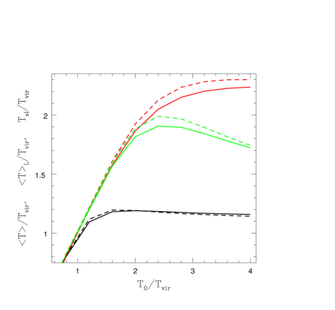
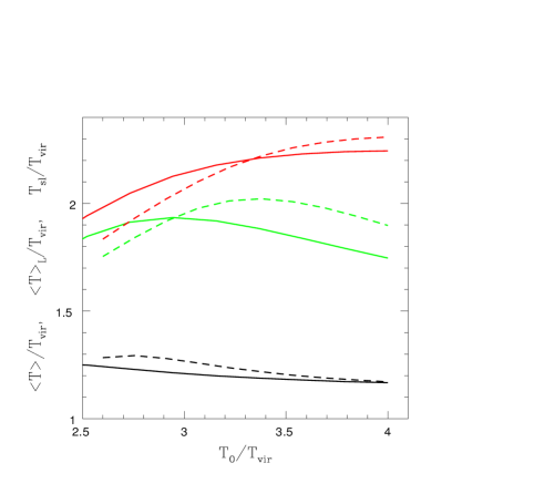
Figure 4: The mass weighted $<T>$ (black), luminosity weighted $<T>_{L}$ (red) and spectroscopic-like $T_{\rm sl}$ (green) temperatures for the truncated quasi-isothermal models (left) and the truncated quasi-polytropic models with $\Gamma=1.2$ (right). Solid lines refer to the $\gamma=0$ potential, dashed lines to the Hernquist potential (see Sect. 3.1 for more details).

2.2.4 Comparison with observed ICM properties

Even though the aim of this work is not to construct models reproducing in detail the observed ICM properties (which is hard within the simple framework of hydrostatic equilibrium of single-phase gas in smooth potential wells), we briefly comment here on how the obtained equilibria compare with observations. In general, the quasi-isothermal and polytropic models, and the TMB models with $\alpha=0$, are similar to “non cool-core” systems, while the $\alpha=1$ and $\alpha=2$ TMB models, where the temperature profile is decreasing towards the center, are similar to “cool-core” systems.

In the family of non cool-core models, quasi-isothermal distributions can be built with arbitrarily low temperatures, becoming more and more similar to the standard isothermal models. Quasi-polytropic models instead, once the truncation potential is fixed, cannot be built with a central temperature smaller than a limit temperature roughly corresponding to the depth of the dark matter potential well. In the past, polytropic models with $\Gamma=1.2$ have been used to reproduce the external regions of ICM observed (e.g., Markevitch et al. 1998, Piffaretti et al. 2005) and simulated (Ostriker et al. 2005).

In the family of cool-core models, TMB distributions with $\alpha=1$ or $\alpha=2$ show temperature profiles in good agreement with those observed by $Chandra$ and $XMM-Newton$ (e.g., Allen et al. 2001, Kaastra et al. 2004, Vikhlinin et al. 2005, 2006); on average, these profiles reach a maximum near $r_{\rm c}$ and then decline at larger radii, reaching $\sim 0.5$ of their peak value near $r\sim 0.5r_{\rm vir}$. In addition, not only the profile shapes of these TMB models are similar to the observed ones, but also their temperature values, when rescaled to the mass-weighted temperature within $r_{500}$ ($T_{500}$), agree with the observed values (as those shown by Viklinin et al. 2006). The relation between $<T>$ and $T_{500}$ will be briefly addressed at the end of Sect. 3.1.

2.3 The abundance profile and the emissivity

In addition to the dark matter potential well and the hydrostatic gas distribution, the third ingredient of our models is the metal distribution. In the numerical code the metal abundance profile is assumed to be stratified according to a formula which generalizes to the ellipsoidal case the observed abundance profiles (Ikebe et al. 2003, De Grandi et al. 2004, Vikhlinin et al. 2005), i.e.

$$Z={Z_{0}\over(1+m_{\rm Z}^{2})^{\zeta}},\quad m_{\rm Z}^{2}={x^{2}\over r_{\rm Z}^{2}}+{y^{2}\over(1-\epsilon)^{2}r_{\rm Z}^{2}}+{z^{2}\over(1-\eta)^{2}r_{\rm Z}^{2}},$$ (24)

where the central metallicity is $Z_{0}=0.8Z_{\odot}$, the slope $\zeta=0.18$ and the metallicity scale-length $r_{\rm Z}=0.04r_{\rm vir}$. In addition, the flattening of the metallicity distribution is the same used for the dark matter distribution. Obviously, we are not attaching any special physical reason to this last assumption, except to have flatter metal distributions in flatter systems, and to reduce the parameter space dimensionality. In any case, we also explored cases where the metals are stratified exactly on isodensity surfaces, i.e. $Z\propto(\rho/\rho_{0})^{\zeta}$, without finding significant differences with the case of eq. (24).

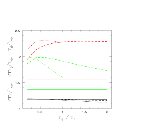
Figure 5: The mass weighted $<T>$ (black), luminosity weighted $<T>_{L}$ (red) and spectroscopic-like $T_{\rm sl}$ (eq. [30], green) temperatures calculated for TMB gas models within the $\gamma=1$ potential, for $\alpha=0$ (dotted lines), $\alpha=1$ (dashed lines) and $\alpha=2$ (solid lines), as a function of $r_{\rm g}/r_{\rm c}$. For $\alpha=2$ the average temperatures are independent of $r_{\rm g}/r_{\rm c}$, consistently with eq. (21) with $\beta=2/3$. For $\alpha=0$ the value of $<T>_{L}/T_{\rm vir}$ is displayed only up to $r_{\rm g}/r_{\rm c}=1$ since for higher $r_{\rm g}/r_{\rm c}$ the central temperatures become very high (Fig. 3).

The emissivity adopted in the code is given by

$${\cal{E}}=n_{e}n_{H}\Lambda(T,Z)\quad$$ (25)

where $n_{e}$ and $n_{H}$ are the number densities of electrons and hydrogen. The cooling function $\Lambda(T,Z)$ has been calculated over the energy interval 0.3–8 keV with the radiative emission code APEC for hot plasmas at the collisional ionization equilibrium (Smith et al. 2001), as available in the XSPEC package (version 12.2.0) for the solar abundance ratios of Grevesse & Sauval (1998). With APEC we have computed a matrix of values for $\Lambda(T,Z)$ for a very large set of temperatures and metallicities. Note that the cooling function can be written as

$$\Lambda(T,Z)=\Lambda(T,0)\left[1+Z\,g(T,Z)\right],$$ (26)

where $Z$ is in solar units, $\Lambda(T,0)$ is the function in the case of no metals, and

$$g(T,Z)\equiv{\Lambda(T,Z)-\Lambda(T,0)\over Z\,\Lambda(T,0)}.$$ (27)

It turned out that the function $g$ is almost exactly independent of $Z$, so that eq. (26) with $g=g(T)$ exploits the nearly perfect linear dependence of the function $\Lambda(T,Z)$ on abundance. In order to speed up the numerical code we computed non-linear fits of the functions $\Lambda(T,0)$ and $g(T)$ valid over the temperature range 0.1–16 keV (with maximum deviations from the APEC values $<1$%) and reported in Appendix B. We remark that $g(T)$ declines steadily with increasing $T$, from $\simeq 42$ down to $\simeq 0.14$, which has the consequence that for high values of $Zg(T)$ then $\Lambda(T,Z)\propto Z_{0}$ and $L_{\rm X}\propto Z_{0}$, while for low values of $Zg(T)$ both $\Lambda(T,Z)$ and $L_{\rm X}$ are independent of $Z_{0}$.

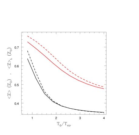
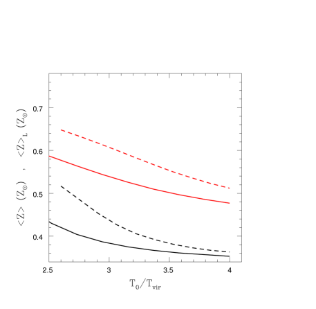
Figure 6: The mass weighted $<Z>$ (black) and luminosity weighted $<Z>_{L}$ (red), calculated for quasi-isothermal equilibria (left) and for quasi-polytropic equilibria with $\Gamma=1.2$ (right), within the $\gamma=0$ (solid lines) and $\gamma=1$ (dashed lines) potentials. The abundance profile is that of eq. (24), with $Z_{0}=0.8Z_{\odot}$.

3 Results

For each model the quantities $<Z>_{L}$ and $<T>_{L}$ are not computed through projection, but directly as volume integrals. In fact, from the Projection Theorem (Appendix A1) eqs. (4)-(5) can be also written as

$$<Z>_{L}=\displaystyle{\int{\cal{E}}[\rho({\bf x}),T({\bf x}),Z({\bf x})]\,Z({\bf x})\,d^{3}{\bf x}\over L_{\rm X}},$$ (28)

and

$$<T>_{L}=\displaystyle{\int{\cal{E}}[\rho({\bf x}),T({\bf x}),Z({\bf x})]\,T({\bf x})\,d^{3}{\bf x}\over L_{\rm X}},$$ (29)

where ${\cal{E}}$ is the emissivity in the 0.3–8 keV band due to gas in the temperature range 0.1-16 keV. As anticipated in the Introduction, for each model we also compute the spectroscopic-like temperature. Following Vikhlinin (2006), this is estimated as

$$T_{\rm sl}=xT_{\rm cont}+(1-x)T_{\rm line},$$ (30)

where $T_{\rm cont}$ and $T_{\rm line}$ are the continuum-based and line-based temperatures for the composite spectrum and $x$ is a parameter that measures the relative contribution of the line and continuum emission to the total flux. To evaluate $T_{\rm cont}$, $T_{\rm line}$ and $x$, three functions of the temperature are needed; these depend on the instrument in use, energy band, redshift and neutral hydrogen absorbing column. As a representative case we chose to simulate observations made with the $Chandra$ CCDs over the 0.3–8 keV band, for a plasma at zero redshift and zero absorbing column. A. Vikhlinin kindly provided us with the tabulated values of the required functions, that we fitted with the same high precision method described in Appendix B and we then inserted in our code. We recall that the method of Vikhlinin (2006) holds for thermal components of $kT{\mathrel{\mathchoice{\lower 2.9pt\vbox{\halign{$\m@th\displaystyle\hfil#\hfil$\cr>\crcr\sim\crcr}}}{\lower 2.9pt\vbox{\halign{$\m@th\textstyle\hfil#\hfil$\cr>\crcr\sim\crcr}}}{\lower 2.9pt\vbox{\halign{$\m@th\scriptstyle\hfil#\hfil$\cr>\crcr\sim\crcr}}}{\lower 2.9pt\vbox{\halign{$\m@th\scriptscriptstyle\hfil#\hfil$\cr>\crcr\sim\crcr}}}}}0.5$ keV. We also computed the estimate of $T_{\rm sl}$ proposed by Mazzotta et al. (2004) for plasma components at $kT{\mathrel{\mathchoice{\lower 2.9pt\vbox{\halign{$\m@th\displaystyle\hfil#\hfil$\cr>\crcr\sim\crcr}}}{\lower 2.9pt\vbox{\halign{$\m@th\textstyle\hfil#\hfil$\cr>\crcr\sim\crcr}}}{\lower 2.9pt\vbox{\halign{$\m@th\scriptstyle\hfil#\hfil$\cr>\crcr\sim\crcr}}}{\lower 2.9pt\vbox{\halign{$\m@th\scriptscriptstyle\hfil#\hfil$\cr>\crcr\sim\crcr}}}}}3$ keV:

$$T_{\rm sl}(\delta)={\int\rho^{2}({\bf x})T^{\delta-1/2}({\bf x})d^{3}{\bf x}\over\int\rho^{2}({\bf x})T^{\delta-3/2}({\bf x})d^{3}{\bf x}},$$ (31)

where $\delta=3/4$ for observations obtained with $Chandra$ and $XMM-Newton$.

It is important to note that if $Z$ and $T$ do not depend on ${\bf x}$, then $<Z>_{L}=<Z>=Z$ and $<T>_{L}=<T>=T_{\rm sl}=T$, even for density distributions depending on ${\bf x}$; otherwise the variously weighted quantities differ, in a way dependent on the spatial distribution of $\rho$, $T$ and $Z$. A quantitative estimate of these differences is the task of the following Sects. 3.1 and 3.2.

For each model all integrals have been calculated numerically with a double-precision code. The integration scheme employs a linear interpolation of the gridpoint-defined variables, and the number of grid points in the positive octant of the $(x\,,y\,,z)$ space is $n_{x}\times n_{y}\times n_{z}=300\times 300\times 300$. Checks of the code have been performed by calculating (with both linearly spaced and logarithmic grids) the total masses of strongly peaked triaxial distributions whose values are known analytically, and also mean value temperatures of special distributions for which the expected values can be calculated analytically (see Section 3.1), obtaining errors ${\mathrel{\mathchoice{\lower 2.9pt\vbox{\halign{$\m@th\displaystyle\hfil#\hfil$\cr<\crcr\sim\crcr}}}{\lower 2.9pt\vbox{\halign{$\m@th\textstyle\hfil#\hfil$\cr<\crcr\sim\crcr}}}{\lower 2.9pt\vbox{\halign{$\m@th\scriptstyle\hfil#\hfil$\cr<\crcr\sim\crcr}}}{\lower 2.9pt\vbox{\halign{$\m@th\scriptscriptstyle\hfil#\hfil$\cr<\crcr\sim\crcr}}}}}$ 0.1%.

3.1 Temperature averages

Figures 4 and 5 show the trend of the mass weighted temperature $<T>$, of the luminosity weighted temperature $<T>_{L}$ and of $T_{\rm sl}$ (eq. [30]), as a function of $T_{0}/T_{\rm vir}$ in the quasi-isothermal and quasi-polytropic cases, and of $r_{\rm g}/r_{\rm c}$ in the TMB case. As for Figs. 1-3, the gravitating mass is a spherical $\gamma=0$ or $\gamma=1$ model with $M=5\times 10^{14}M_{\odot}$; also the range of $T_{0}/T_{\rm vir}$ and $r_{\rm g}/r_{\rm c}$ is the same used for Figs. 1-3.

A first general result is that at this mass $M$ the two $T_{\rm sl}$ estimates of eqs. (30) and (31) agree within $\sim 10$% for all the explored models. The reasons for this are the relatively flat shape of the temperature profiles that are obtained by hydrostatic equilibria in smooth potential wells; the not too peaked metallicity distribution; and finally the virial temperature of the gas ($T_{\rm vir}=2.3$ keV) that is not much lower than 3 keV (i.e., the declared limit of applicability of the Mazzotta et al.’s $T_{\rm sl}$). A similar finding has been reported by Rasia et al. (2008). In fact, for models with strongly peaked metallicity distributions, or with much lower mass (e.g., $M=10^{14}M_{\odot}$ and $T_{\rm vir}=0.8$ keV) we found that the two spectroscopic temperatures are clearly different, and the Mazzotta et al. (2004) estimate would be higher than that of Vikhlinin (2006) (up to 20% in the explored $T_{0}/T_{\rm vir}$ range, for the quoted mass $M$).

Finally, it is useful to mention the relation between $<T>$ and $T_{500}$ (see end of Sect. 2.2.4), since the temperature profile is generally recovered from observations out to radii smaller than $r_{\rm vir}$, typically out to $r_{500}$ with the most sensitive observations (e.g., Viklinin et al. 2006). The calculation of the $T_{500}/<T>$ ratio for all our models confirmed the expectation that the hotter is the central region with respect to the outer one, the higher is this ratio. In fact, we found for quasi-isothermal models $T_{500}=(1\div 1.5)<T>$, as $T_{0}/T_{\rm vir}$ goes from 0.4 to 4; for quasi-polytropic models $T_{500}=(1\div 1.4)<T>$, as $T_{0}/T_{\rm vir}$ goes from 2.6 to 4. For TMB models, $T_{500}/<T>$ varies respectively between 1.3 and 1.5, and between 1.3 and 1.6, for $\alpha=1$ and $\alpha=0$, as $r_{\rm g}/r_{\rm c}$ varies between 0.2 to 2; for $\alpha=2$, $T_{500}/<T>=1.3$, the lowest value, a consequence of its cold central region.

3.1.1 Quasi-isothermal and polytropic models

We first discuss Fig. 4. For $T_{0}{\mathrel{\mathchoice{\lower 2.9pt\vbox{\halign{$\m@th\displaystyle\hfil#\hfil$\cr>\crcr\sim\crcr}}}{\lower 2.9pt\vbox{\halign{$\m@th\textstyle\hfil#\hfil$\cr>\crcr\sim\crcr}}}{\lower 2.9pt\vbox{\halign{$\m@th\scriptstyle\hfil#\hfil$\cr>\crcr\sim\crcr}}}{\lower 2.9pt\vbox{\halign{$\m@th\scriptscriptstyle\hfil#\hfil$\cr>\crcr\sim\crcr}}}}}T_{\rm vir}$, $<T>_{L}$ and $T_{\rm sl}$ are both higher (up to a factor of $\sim 2$) than the mass-weighted temperature $<T>$, because they are dominated by the hotter central regions. For quasi-isothermal models with $T_{0}{\mathrel{\mathchoice{\lower 2.9pt\vbox{\halign{$\m@th\displaystyle\hfil#\hfil$\cr<\crcr\sim\crcr}}}{\lower 2.9pt\vbox{\halign{$\m@th\textstyle\hfil#\hfil$\cr<\crcr\sim\crcr}}}{\lower 2.9pt\vbox{\halign{$\m@th\scriptstyle\hfil#\hfil$\cr<\crcr\sim\crcr}}}{\lower 2.9pt\vbox{\halign{$\m@th\scriptscriptstyle\hfil#\hfil$\cr<\crcr\sim\crcr}}}}}T_{\rm vir}$, instead, the 3 temperatures almost coincide, because the gas is nearly isothermal (see Fig. 1). Overall, $T_{\rm sl}$ and $<T>_{L}$ agree very well up to $T_{0}\simeq 2T_{\rm vir}$. Starting from $T_{0}{\mathrel{\mathchoice{\lower 2.9pt\vbox{\halign{$\m@th\displaystyle\hfil#\hfil$\cr>\crcr\sim\crcr}}}{\lower 2.9pt\vbox{\halign{$\m@th\textstyle\hfil#\hfil$\cr>\crcr\sim\crcr}}}{\lower 2.9pt\vbox{\halign{$\m@th\scriptstyle\hfil#\hfil$\cr>\crcr\sim\crcr}}}{\lower 2.9pt\vbox{\halign{$\m@th\scriptscriptstyle\hfil#\hfil$\cr>\crcr\sim\crcr}}}}}2T_{\rm vir}$, $<T>_{L}$ is larger than $T_{\rm sl}$, a tendency that becomes stronger with increasing $T_{0}/T_{\rm vir}$: this is due to fact that $T_{\rm sl}$ is biased towards the lower values of the range of temperatures [e.g. $T_{\rm sl}(3/4)$ weights each thermal component by $\rho^{2}T^{-3/4}$ instead of by $\rho^{2}\Lambda(T)\sim\rho^{2}T^{1/2}$].

At high $T_{0}$ the size of the discrepancy between $<T>$ and $<T>_{L}$ or $T_{\rm sl}$ compares well with the analytical predictions based on the asymptotic profiles (14), (20). From these expressions, defining $\Psi\equiv\phi/\phi_{0}$, the limit values of $<T>$ and $T_{\rm sl}(\delta)$, both in the quasi-isothermal and quasi-polytropic cases, are

$$<T>={|\phi_{0}|\mu m_{\rm H}\over 2k}{\int(\Psi-\Psi_{\rm t})^{2}d^{3}{\bf x}\over\int(\Psi-\Psi_{\rm t})d^{3}{\bf x}},$$ (32)

and

$$T_{\rm sl}(\delta)={|\phi_{0}|\mu m_{\rm H}\over 2k}{\int(\Psi-\Psi_{\rm t})^{3/2+\delta}d^{3}{\bf x}\over\int(\Psi-\Psi_{\rm t})^{1/2+\delta}d^{3}{\bf x}},$$ (33)

which are independent of $T_{0}$. In particular, note that $T_{\rm sl}(2)$ corresponds to the case of pure bremsstrahlung emission, which is similar to the emission described by our adopted cooling function, at least for high temperatures.

The analytical solution of the integrals (32) and (33), for spherical $\gamma=1$ models with truncation at the virial radius, gives $<T>\simeq 1.11T_{\rm vir}$, $T_{\rm sl}(2)\simeq 2.29T_{\rm vir}$ and $T_{\rm sl}(3/4)\simeq 1.30T_{\rm vir}$. These values are close to those shown by $<T>$ and $<T>_{L}$ at $T_{0}\simeq 4T_{\rm vir}$ (Fig. 4); $T_{\rm sl}(3/4)$ instead is still far from its limit value, even though it has already started decreasing. As long as $<T>_{L}$ can be considered similar to $T_{\rm sl}(2)$, then $T_{\rm sl}(3/4)$ is predicted to tend to $\simeq 0.6<T>_{L}$ (which was verified with numerical models not presented here). The same calculations at the limit of high $T_{0}$ for the $\gamma=0$ potential give $<T>\simeq 1.13T_{\rm vir}$, $T_{\rm sl}(2)\simeq 2.27T_{\rm vir}$ and $T_{\rm sl}(3/4)\simeq 1.31T_{\rm vir}$; these values are very similar to those for $\gamma=1$, in agreement with the close location of the solid and dashed lines in Fig. 4.

3.1.2 TMB models

The TMB cases (Fig. 5) are more varied. The first result is that $<T>$ (black lines) remains almost constant for different $r_{\rm g}/r_{\rm c}$, at a value nearly independent of $\alpha$. Analytic integration for $\alpha=2$ shows that $<T>=1.18T_{\rm vir}$, in agreement with the numerical result in Fig. 5. The second result is that again $T_{\rm sl}$ and $<T>_{L}$ overestimate $<T>$.

$T_{\rm sl}$ (green lines) decreases steeply with increasing $r_{\rm g}/r_{\rm c}$ for $\alpha=0$, because the density in the central hotter regions decreases by almost an order of magnitude, while it is increasing in the colder external region. This same trend is again present, though milder, for the models with $\alpha=1$. As discussed in Appendix A2, without a cut at low temperatures $T_{\rm sl}(\delta)$ diverges for the $\alpha=2$ models; therefore a cut at $kT=0.1$ keV (which excludes the cold central regions where $\rho\propto r^{-2}$) has been adopted to produce Fig. 5. $<T>_{L}$ does not suffer from this problem, because of the low temperature cut in the cooling function. $<T>_{L}$ is higher than $T_{\rm sl}$ (for the same $\alpha$) as in the quasi-isothermal and quasi-polytropic models, and for the same reason of being $T_{\rm sl}$ biased towards the lower values of the temperature range.

3.1.3 Changing the dark mass amount and shape

For all models (quasi-isothermal, polytropic and TMB) we investigated the effects of changing the total mass $M$ and of flattening the dark mass distribution. We found that all the trends in Figs. 4 and 5 remain the same with a different total mass $M$ and shape.

For what is concerning the values of the average temperatures, $<T>_{L}/T_{\rm vir}$ and $T_{\rm sl}/T_{\rm vir}$ remain the same within few ($\sim 5$) percent, for $M\geq 3\times 10^{14}M_{\odot}$. The only exception is $T_{\rm sl}/T_{\rm vir}$ calculated according to Vikhlinin (2006) for the TMB models with $\alpha=2$, that decreases by 13% going from $M=1.4\times 10^{15}M_{\odot}$ to $M=3\times 10^{14}M_{\odot}$. $<T>/T_{\rm vir}$ and $T_{\rm sl}(\delta)/T_{\rm vir}$, instead, are independent of $M$ for all models, as can be proved analytically: the curves in Figs. 4 and 5 depend (for all the other parameters fixed) only on $T_{0}/T_{\rm vir}$ or $r_{\rm g}/r_{\rm c}$, and on $\epsilon$ and $\eta$.

For a fixed mass $M$ ($\geq 3\times 10^{14}M_{\odot}$), we then changed the values of $\epsilon$ and $\eta$ from zero to 0.1 and 0.3, which produces a flat E7-like shape, and up to 0.5 and 0.5. The values of all the average temperatures, when rescaled for the different $T_{\rm vir}$, remain the same within 5%. Again the largest variation is that of $T_{\rm sl}/T_{\rm vir}$ calculated according to Vikhlinin (2006) for the TMB models with $\alpha=2$, that increases by 13% going from the spherical to the $\epsilon=\eta=0.5$ shape (that corresponds to a very prolate ellipsoid).

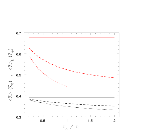
Figure 7: The mass weighted $<Z>$ (black) and luminosity weighted $<Z>_{L}$ (red) abundances calculated for TMB models within the $\gamma=1$ potential, for $\alpha=0$ (dotted lines), $\alpha=1$ (dashed lines) and $\alpha=2$ (solid lines), as a function of $r_{g}/r_{c}$. For $\alpha=2$ the density and temperature profiles are independent of $r_{g}/r_{\rm c}$, and so are $<Z>$ and $<Z>_{L}$; for $\alpha=0$, only the values up to $r_{\rm g}/r_{\rm c}=1$ are displayed, as for Fig. 5.

3.2 Abundance averages

Figures 6 and 7 show the trend of $<Z>$ and $<Z>_{L}$ as a function of $T_{0}/T_{\rm vir}$ (for quasi-isothermal and quasi-polytropic models) or $r_{g}/r_{\rm c}$ (for TMB models), for the same total mass $M$ and potentials used in the previous figures, and for the abundance profile (24), with the parameter values specified below that equation. These figures show that $<Z>_{L}$ (red lines) always overestimates $<Z>$ (black lines), a result of the larger weight that central regions have in the calculation of $<Z>_{L}$. For all models $<Z>$ and $<Z>_{L}$ decrease with $T_{0}/T_{\rm vir}$ or $r_{\rm g}/r_{\rm c}$ increasing; this is explained by the fixed metallicity profile coupled with gas density profiles that become flatter (Figs. 1 and 2), so that the central regions where the abundance is highest become less and less important in the integrals of eqs. (1) and (28) (except for the TMB $\alpha=2$ models, where the density profile is independent of $r_{\rm g}/r_{\rm c}$). The steeper density profiles are those of the isothermal models with $T_{0}<2T_{\rm vir}$ (Fig. 1), therefore the decrease of $<Z>$ and $<Z>_{L}$ at increasing $T_{0}$ is more pronounced in this range of temperatures.

In general, the details of the discrepancy between $<Z>$ and $<Z>_{L}$, and its trend with $T_{0}/T_{\rm vir}$ or $r_{g}/r_{\rm c}$, depend on how the density, temperature and abundance profiles differ from each other. The overestimate obtained by using luminosity weighted abundances is stronger for steeper gas density profiles. For example, the $\gamma=0$ models have a slightly flatter density profile at the center than the $\gamma=1$ ones, so that the discrepancy between $<Z>$ and $<Z>_{L}$ is in general slightly smaller for $\gamma=0$ than for $\gamma=1$. A similar behavior is presented by TMB models. The profiles in this family may have a drop in temperature at the center, and consequently a steep increase in density, that is more pronounced for $\alpha=2$ (Fig. 3). Figure 7 reflects this fact, showing the largest overestimate of $<Z>_{L}$ among TMB models for $\alpha=2$, while the smallest is that of $\alpha=0$ models.

In summary, considering all our models $<Z>_{L}/<Z>$ lies in a quite small range: $1.1{\mathrel{\mathchoice{\lower 2.9pt\vbox{\halign{$\m@th\displaystyle\hfil#\hfil$\cr<\crcr\sim\crcr}}}{\lower 2.9pt\vbox{\halign{$\m@th\textstyle\hfil#\hfil$\cr<\crcr\sim\crcr}}}{\lower 2.9pt\vbox{\halign{$\m@th\scriptstyle\hfil#\hfil$\cr<\crcr\sim\crcr}}}{\lower 2.9pt\vbox{\halign{$\m@th\scriptscriptstyle\hfil#\hfil$\cr<\crcr\sim\crcr}}}}}<Z>_{L}/<Z>{\mathrel{\mathchoice{\lower 2.9pt\vbox{\halign{$\m@th\displaystyle\hfil#\hfil$\cr<\crcr\sim\crcr}}}{\lower 2.9pt\vbox{\halign{$\m@th\textstyle\hfil#\hfil$\cr<\crcr\sim\crcr}}}{\lower 2.9pt\vbox{\halign{$\m@th\scriptstyle\hfil#\hfil$\cr<\crcr\sim\crcr}}}{\lower 2.9pt\vbox{\halign{$\m@th\scriptscriptstyle\hfil#\hfil$\cr<\crcr\sim\crcr}}}}}1.6$ for quasi-isothermal models, $1.25{\mathrel{\mathchoice{\lower 2.9pt\vbox{\halign{$\m@th\displaystyle\hfil#\hfil$\cr<\crcr\sim\crcr}}}{\lower 2.9pt\vbox{\halign{$\m@th\textstyle\hfil#\hfil$\cr<\crcr\sim\crcr}}}{\lower 2.9pt\vbox{\halign{$\m@th\scriptstyle\hfil#\hfil$\cr<\crcr\sim\crcr}}}{\lower 2.9pt\vbox{\halign{$\m@th\scriptscriptstyle\hfil#\hfil$\cr<\crcr\sim\crcr}}}}}<Z>_{L}/<Z>{\mathrel{\mathchoice{\lower 2.9pt\vbox{\halign{$\m@th\displaystyle\hfil#\hfil$\cr<\crcr\sim\crcr}}}{\lower 2.9pt\vbox{\halign{$\m@th\textstyle\hfil#\hfil$\cr<\crcr\sim\crcr}}}{\lower 2.9pt\vbox{\halign{$\m@th\scriptstyle\hfil#\hfil$\cr<\crcr\sim\crcr}}}{\lower 2.9pt\vbox{\halign{$\m@th\scriptscriptstyle\hfil#\hfil$\cr<\crcr\sim\crcr}}}}}1.45$ for quasi-polytropic models, and $1.3{\mathrel{\mathchoice{\lower 2.9pt\vbox{\halign{$\m@th\displaystyle\hfil#\hfil$\cr<\crcr\sim\crcr}}}{\lower 2.9pt\vbox{\halign{$\m@th\textstyle\hfil#\hfil$\cr<\crcr\sim\crcr}}}{\lower 2.9pt\vbox{\halign{$\m@th\scriptstyle\hfil#\hfil$\cr<\crcr\sim\crcr}}}{\lower 2.9pt\vbox{\halign{$\m@th\scriptscriptstyle\hfil#\hfil$\cr<\crcr\sim\crcr}}}}}<Z>_{L}/<Z>{\mathrel{\mathchoice{\lower 2.9pt\vbox{\halign{$\m@th\displaystyle\hfil#\hfil$\cr<\crcr\sim\crcr}}}{\lower 2.9pt\vbox{\halign{$\m@th\textstyle\hfil#\hfil$\cr<\crcr\sim\crcr}}}{\lower 2.9pt\vbox{\halign{$\m@th\scriptstyle\hfil#\hfil$\cr<\crcr\sim\crcr}}}{\lower 2.9pt\vbox{\halign{$\m@th\scriptscriptstyle\hfil#\hfil$\cr<\crcr\sim\crcr}}}}}1.7$ for TMB models.

3.2.1 Changing the dark mass amount and shape

For all models presented in this paper it can be proved that $<Z>$ is independent of $M$, while it depends on $T_{0}/T_{\rm vir}$ or $r_{\rm g}/r_{\rm c}$, and $\epsilon$ and $\eta$. As a consequence, the values of $<Z>$ in Figs. 6–7 keep the same for all dark masses $M$ when the metallicity distribution (23) is used with the specified parameters. $<Z>_{L}$ remains almost identical, for $M\geq 3\times 10^{14}M_{\odot}$, with the largest variation for the highest $T_{0}/T_{\rm vir}$ and $r_{\rm g}/r_{\rm c}$ of just 2%. These small variations are accounted for by the fact that the gas emissivity is not a pure power-law in temperature.

As for the temperatures, we also investigated the effect of flattening of the mass distribution. $<Z>$ and $<Z>_{L}$ become smaller when increasing the flattening with respect to the spherical case, which is explained by more and more gas mass being displaced at larger distances from the center, where the abundance is lower. When changing the values of $\epsilon$ and $\eta$ from zero to (0.5, 0.5), for the range of $T_{0}/T_{\rm vir}$ of Fig. 6 and of $r_{\rm g}/r_{\rm c}$ of Fig. 7, $<Z>$ decreases by ${\mathrel{\mathchoice{\lower 2.9pt\vbox{\halign{$\m@th\displaystyle\hfil#\hfil$\cr<\crcr\sim\crcr}}}{\lower 2.9pt\vbox{\halign{$\m@th\textstyle\hfil#\hfil$\cr<\crcr\sim\crcr}}}{\lower 2.9pt\vbox{\halign{$\m@th\scriptstyle\hfil#\hfil$\cr<\crcr\sim\crcr}}}{\lower 2.9pt\vbox{\halign{$\m@th\scriptscriptstyle\hfil#\hfil$\cr<\crcr\sim\crcr}}}}}16$%, and $<Z>_{L}$ by ${\mathrel{\mathchoice{\lower 2.9pt\vbox{\halign{$\m@th\displaystyle\hfil#\hfil$\cr<\crcr\sim\crcr}}}{\lower 2.9pt\vbox{\halign{$\m@th\textstyle\hfil#\hfil$\cr<\crcr\sim\crcr}}}{\lower 2.9pt\vbox{\halign{$\m@th\scriptstyle\hfil#\hfil$\cr<\crcr\sim\crcr}}}{\lower 2.9pt\vbox{\halign{$\m@th\scriptscriptstyle\hfil#\hfil$\cr<\crcr\sim\crcr}}}}}14$%. Smaller variations are obtained for more reasonable flattenings, as for example of the order of $\sim 5$% for $\epsilon$ and $\eta$ equal to 0.1, 0.3.

4 Summary and conclusions

In this work we have compared the values of mass and luminosity weighted metallicity and temperature, for a large set of hydrostatic gas distributions, some of which resemble those typical of the intracluster and intragroup media. In addition, we also computed the temperature that would be derived from observed spectra (the so-called spectroscopic-like temperature) by using two recently proposed methods for its estimate. The results of this analysis are useful for distant groups/clusters, or in general for systems with a low number of observed counts, where only global average values can be recovered from observations.

This study is based on a few steps. First, the potential well of triaxial dark matter halos, with different density slopes and adjustable flattenings, was built analytically by means of homeoidal expansion, which gives a simple yet accurate analytical approximation of the true potential. In the second step we showed how to construct hydrostatic analytical solutions for triaxial truncated density distributions, and presented the equilibrium configurations in the quasi-isothermal and quasi-polytropic cases, and for a family of modified $\beta$ models. In the third step we superimposed a metallicity distribution derived from observations of the ICM/IGM. Finally, the gas radiative properties were computed by using the cooling function $\Lambda(T,Z)$ appropriate for our range of gas temperatures and a chosen sensitivity band of 0.3–8 keV. Mass and luminosity weighted temperature and abundances for the models were then obtained, thanks to the Projection Theorem.

The main results can be summarized as follows.

• The quasi-isothermal and polytropic models show gas density and temperature profiles similar to those observed for non-cool core clusters, while those of TMB models with $\alpha=1$ or $\alpha=2$ resemble cool-core clusters. In particular the temperature profiles of the latter TMB models, when rescaled to $T_{500}$, compare well in shape and normalization with observed profiles. In general, $<T>/T_{500}$ ranges between 1 and 1.5, and it is 1.3 for TMB models with $\alpha=2$.

• The luminosity-weighted temperature $<T>_{L}$ overestimates $<T>$ up to a factor of $\sim 2$, and the discrepancies increase with increasing gas temperature (scaled by $T_{\rm vir}$) for quasi-isothermal and polytropic models, or for increasing $r_{\rm g}/r_{\rm c}$ for TMB models. For these latter models with $\alpha=2$ the overestimate is milder (a factor of $\simeq 1.3$).

• $T_{\rm sl}$ always provides a less serious overestimate of $<T>$ than $<T>_{L}$. The discrepancy bewteen $T_{\rm sl}$ and $<T>$ becomes smaller for increasing $T_{0}/T_{\rm vir}$ and for increasing $r_{\rm g}/r_{\rm c}$.

• The exception to a general overestimate of $<T>$ is that of ”cold” ($T_{0}{\mathrel{\mathchoice{\lower 2.9pt\vbox{\halign{$\m@th\displaystyle\hfil#\hfil$\cr<\crcr\sim\crcr}}}{\lower 2.9pt\vbox{\halign{$\m@th\textstyle\hfil#\hfil$\cr<\crcr\sim\crcr}}}{\lower 2.9pt\vbox{\halign{$\m@th\scriptstyle\hfil#\hfil$\cr<\crcr\sim\crcr}}}{\lower 2.9pt\vbox{\halign{$\m@th\scriptscriptstyle\hfil#\hfil$\cr<\crcr\sim\crcr}}}}}1.2T_{\rm vir}$) quasi-isothermal models, where the three temperatures $<T>$, $<T>_{L}$ and $T_{\rm sl}$ are very similar. Also, $<T>_{L}$ and $T_{\rm sl}$ keep close up to $T_{0}\simeq 2T_{\rm vir}$, and depart for higher $T_{0}/T_{\rm vir}$.

• When changing the total dark mass $M$, the general behavior of $<T>$, $<T>_{L}$ and $T_{\rm sl}$ described above remains the same. The values of $<T>_{L}/T_{\rm vir}$ and $T_{\rm sl}/T_{\rm vir}$ turn out to keep within $5$% by changing $M$, for the range of masses typical of large groups and clusters ($M\geq 3\times 10^{14}M_{\odot}$). $<T>/T_{\rm vir}$ is instead independent of $M$.

• In the explored range of triaxiality, flattening effects are not strong: the average temperatures normalized to $T_{\rm vir}$ remain the same within 5%.

• The only exception to the small (${\mathrel{\mathchoice{\lower 2.9pt\vbox{\halign{$\m@th\displaystyle\hfil#\hfil$\cr<\crcr\sim\crcr}}}{\lower 2.9pt\vbox{\halign{$\m@th\textstyle\hfil#\hfil$\cr<\crcr\sim\crcr}}}{\lower 2.9pt\vbox{\halign{$\m@th\scriptstyle\hfil#\hfil$\cr<\crcr\sim\crcr}}}{\lower 2.9pt\vbox{\halign{$\m@th\scriptscriptstyle\hfil#\hfil$\cr<\crcr\sim\crcr}}}}}5$%) variance with a change of shape or mass is given by the ”cool-core” models (TMB models with $\alpha=2$): the increase of $T_{\rm sl}/T_{\rm vir}$ can be as large as 13% going from $M=3\times 10^{14}M_{\odot}$ to $M=1.4\times 10^{15}M_{\odot}$, or from spherical to $\epsilon=\eta=0.5$ at fixed $M$.

• The luminosity weighted $<Z>_{L}$ overestimates the mass weighted average abundance $<Z>$. For quasi-polytropic and quasi-isothermal models with $T_{0}\geq 2.6T_{\rm vir}$ we found that $1.3{\mathrel{\mathchoice{\lower 2.9pt\vbox{\halign{$\m@th\displaystyle\hfil#\hfil$\cr<\crcr\sim\crcr}}}{\lower 2.9pt\vbox{\halign{$\m@th\textstyle\hfil#\hfil$\cr<\crcr\sim\crcr}}}{\lower 2.9pt\vbox{\halign{$\m@th\scriptstyle\hfil#\hfil$\cr<\crcr\sim\crcr}}}{\lower 2.9pt\vbox{\halign{$\m@th\scriptscriptstyle\hfil#\hfil$\cr<\crcr\sim\crcr}}}}}<Z>_{L}/<Z>{\mathrel{\mathchoice{\lower 2.9pt\vbox{\halign{$\m@th\displaystyle\hfil#\hfil$\cr<\crcr\sim\crcr}}}{\lower 2.9pt\vbox{\halign{$\m@th\textstyle\hfil#\hfil$\cr<\crcr\sim\crcr}}}{\lower 2.9pt\vbox{\halign{$\m@th\scriptstyle\hfil#\hfil$\cr<\crcr\sim\crcr}}}{\lower 2.9pt\vbox{\halign{$\m@th\scriptscriptstyle\hfil#\hfil$\cr<\crcr\sim\crcr}}}}}1.5$. This ratio extends over a larger range ($1.1{\mathrel{\mathchoice{\lower 2.9pt\vbox{\halign{$\m@th\displaystyle\hfil#\hfil$\cr<\crcr\sim\crcr}}}{\lower 2.9pt\vbox{\halign{$\m@th\textstyle\hfil#\hfil$\cr<\crcr\sim\crcr}}}{\lower 2.9pt\vbox{\halign{$\m@th\scriptstyle\hfil#\hfil$\cr<\crcr\sim\crcr}}}{\lower 2.9pt\vbox{\halign{$\m@th\scriptscriptstyle\hfil#\hfil$\cr<\crcr\sim\crcr}}}}}<Z>_{L}/<Z>{\mathrel{\mathchoice{\lower 2.9pt\vbox{\halign{$\m@th\displaystyle\hfil#\hfil$\cr<\crcr\sim\crcr}}}{\lower 2.9pt\vbox{\halign{$\m@th\textstyle\hfil#\hfil$\cr<\crcr\sim\crcr}}}{\lower 2.9pt\vbox{\halign{$\m@th\scriptstyle\hfil#\hfil$\cr<\crcr\sim\crcr}}}{\lower 2.9pt\vbox{\halign{$\m@th\scriptscriptstyle\hfil#\hfil$\cr<\crcr\sim\crcr}}}}}1.6$) for colder quasi-isothermal models ($T_{0}{\mathrel{\mathchoice{\lower 2.9pt\vbox{\halign{$\m@th\displaystyle\hfil#\hfil$\cr<\crcr\sim\crcr}}}{\lower 2.9pt\vbox{\halign{$\m@th\textstyle\hfil#\hfil$\cr<\crcr\sim\crcr}}}{\lower 2.9pt\vbox{\halign{$\m@th\scriptstyle\hfil#\hfil$\cr<\crcr\sim\crcr}}}{\lower 2.9pt\vbox{\halign{$\m@th\scriptscriptstyle\hfil#\hfil$\cr<\crcr\sim\crcr}}}}}2T_{\rm vir}$). TMB models show their smallest overestimate ($\simeq 1.4$) for $\alpha=0$, and the largest ($\simeq 1.7$) for $\alpha=2$, that repoduces the case of ”cool core” ICM/IGM.

• Similarly to what found for $<T>$, an $M$ variation has no effect on $<Z>$, and a negligible effect on $<Z>_{L}$. The effect of flattening is present, but it is not very important. For $(\epsilon,\eta)$ equal to (0.1, 0.3) and (0.5, 0.5), $<Z>$ and $<Z>_{L}$ decrease by $\leq$few %, and by $\leq 13$% respectively.

Thus, we have shown that when deprojection is not feasible or robust (as in the case of distant objects, significant deviations from spherical symmetry, etc.), the alternative approach of considering the global average values of temperature and abundance, obtained as surface integrals over the image, has the advantage over deprojection of being independent of the shape of the system and of the relative orientation to the observer, but in presence of non-uniform metallicity and temperature distributions it must be calibrated by computing the appropriate correcting factors, as those determined in this paper. It would be interesting to apply both methods (deprojection vs. surface average) to real systems with detailed observations, and to compare the results.

Appendix A Analytical results

A.1 The Projection Theorem

The numerical integrations performed in this paper are based on a very simple but far-reaching mathematical identity holding between volume and surface integrals of projected properties of “transparent” systems of general shape (e.g., see Ciotti 2000). In the present context, let us consider a property $P({\bf x})$ (for example the ICM temperature or metallicity), associated with a field $\nu({\bf x})$ (for example the ICM emissivity) acting as a “weight”. Without loss of generality, we can suppose the line-of-sight to coincide with the $z$-axis, so $(x,y)$ is the projection plane. The weighted projection is naturally defined as

$$\Sigma(x,y)\times P_{\rm pr}(x,y)\equiv\int_{-\infty}^{\infty}\nu({\bf x})\,P({\bf x})\,dz,$$ (34)

where $\Sigma(x,y)=\int_{-\infty}^{\infty}\nu({\bf x})\,dz$. From the identity $\int\Sigma\times P_{\rm pr}\,dx\,dy=\int\nu({\bf x})\,P({\bf x})\,d^{3}{\bf x}$, it follows that

$$<P>_{\nu}\equiv\frac{\displaystyle\int\Sigma\times P_{\rm pr}\,dx\,dy}{\displaystyle\int\Sigma\,dx\,dy}=\frac{\displaystyle\int\nu({\bf x})\,P({\bf x})d^{3}{\bf x}}{\displaystyle\int\nu({\bf x})\,d^{3}{\bf x}},$$ (35)

where the integrals that appear in this definition extend on the whole image. In practice, the surface weighted integral of a projected property coincides with the volume weigthed integral of this property; in turns, this proves that $<P>_{\nu}$ is independent of the viewing angle.

A.2 The density approach

As well known, for a gas in hydrostatic equilibrium in a potential well $\phi({\bf x})$

$$\nabla p=-\rho\nabla\phi,$$ (36)

and the density, temperature and pressure distributions are stratified on the equipotential surfaces, i.e., $\rho=\rho(\phi)$, $p=p(\phi)$, and $T=T(\phi)$, so that the gas is barotropic. In standard applications some relation $p(\rho)$ is assigned, and eq. (A3) is solved. In the density approach instead the functional form $\rho(\phi)$ is assigned. In this case it is trivial to prove that the function

$$H(\phi)\equiv\int_{\phi}^{0}\rho(t)\,dt$$ (37)

satisfies the identity $\nabla H=-\rho(\phi)\nabla\phi$, and so integrating eq. (A3) over an arbitrary path it follows that

$$p({\bf x})-p_{*}=H[\phi({\bf x})]-H[\phi_{*}],$$ (38)

where $p_{*}$ and $\phi_{*}$ are the pressure and potential values at some reference position ${\bf x}_{*}$. For untruncated models in halos of finite mass the natural choice is to set $p_{*}=0$ and $\phi_{*}=0$ at ${\bf x}_{*}=\infty$. For models as those considered in Sect. 2.2, with a finite value of the central potential $\phi_{0}$ and a truncated density $\rho-\rho_{\rm t}$, where $\rho_{\rm t}=\rho(\phi_{\rm t})$, it is natural to set $p_{*}=p_{t}=0$, so that eq. (A5) becomes

$$p({\bf x})=|\phi_{0}|\left[\tilde{H}(\Psi)-\tilde{H}(\Psi_{\rm t})-\rho_{\rm t}\times(\Psi-\Psi_{\rm t})\right],$$ (39)

where $\Psi\equiv\phi/\phi_{0}$ and $\tilde{H}(\Psi)=\int_{0}^{\Psi}\rho(\Psi)d\Psi$.

The simple idea behind the density approach is to choose a spherical gas density distribution $\rho(r)$ with the desired radial profile, and a spherical potential $\phi(r)$. Due to the monotonicity of the potential (guaranteed by Gauss theorem), it is always possible (in principle) to eliminate the radius between the two distributions, thus obtaining $\rho(\phi)$, and the function $H$. In the second step one deform the spherical potential (for example by using homeoidal expansion as in this paper, or with the complex shift method described in Ciotti & Giampieri 2007, or by functional substitution as in the Miyamoto-Nagai 1980 disk case) but assumes that the function $\rho(\phi)$ is the same as in the spherical case. As a consequence, the function $H$ is still exact, while the deformed density profile is more and more similar to the spherical initial distribution for smaller and smaller potential deformations.

In the family of models presented in Sect. 2.2.3, remarkably simple explicit cases are obtained for $\beta=2/3$ and $\alpha=0,1,2$. In particular, after defining $\Psi$ as in equation (15), for $\alpha=0$ we obtain

$${\tilde{H}(\Psi)\over\rho_{0}} = {b^{2}\,\Psi\over b^{2}+1}+{b(1-b^{2})\over(b^{2}+1)^{2}}{\rm arctan}{b\Psi\over 1-\Psi}+$$ (41)

$${b^{2}\log[(1-\Psi)^{2}+b^{2}\Psi^{2}]\over(b^{2}+1)^{2}},$$

for $\alpha=1$

$${\tilde{H}(\Psi)\over\rho_{0}} = b^{2}{1-\sqrt{(1-\Psi)^{2}+b^{2}\Psi^{2}}\over b^{2}+1}+$$ (44)

$$b\log{b\psi+\sqrt{(1-\Psi)^{2}+b^{2}\Psi^{2}}\over 1-\Psi}+{b^{2}(2+b^{2})\over(b^{2}+1)^{3/2}}\times$$

$$\log{{1-(1+b^{2})\Psi+\sqrt{1+b^{2}}\sqrt{(1-\Psi)^{2}+b^{2}\Psi^{2}}}\over 1+\sqrt{1+b^{2}}},$$

and finally

$${\tilde{H}(\Psi)\over\rho_{0}}=b^{2}{\Psi(2-\Psi)\over 1-\Psi}+2b^{2}\log(1-\Psi)$$ (45)

for $\alpha=2$.

It can be easily proved, for example by series expansion and by order matching of the hydrostatic equation near the origin that the equilibrium temperature for $r\to 0$ converges to a positive value for $\alpha=0$, while for $\alpha>0$ it vanishes as $r^{\alpha}$ ($0<\alpha<1$), as $-r\log r$ ($\alpha=1$), and finally as $r$ ($\alpha>1$). In particular, in the $\alpha=2$ models, the vanishing of temperature near the center is not strong enough to compensate the density (square) increase as $r^{-4}$, and this leads to a divergent denominator in the definition of $T_{\rm sl}(\delta)$ for $\delta<5/2$.

Appendix B The cooling function

The functions $\Lambda(T,0)$ (in units of $10^{-24}$ erg cm³ s^-1) and $g(T)$ (dimensionless) appearing in eq. (26) describe the cooling function over the 0.3–8 keV band for plasmas in the temperature range $kT=0.1-16$ keV and with the abundance ratios of Grevesse & Sauval (1998). In order to speed up the numerical integrations, in the code we use the following non-linear fits (the Padé approximants) of the numerical values produced with APEC

$$\Lambda(T,0)={a+bT+cT^{2}+dT^{3}+eT^{4}\over f+gT+hT^{2}+iT^{3}+lT^{4}+mT^{5}},$$ (46)

and

$$g(T)={a+bT+cT^{2}+dT^{3}+eT^{4}+fT^{5}+gT^{6}\over h+iT+lT^{2}+mT^{3}+nT^{4}+oT^{5}+pT^{6}}.$$ (47)

In the expressions above $T$ is expressed in keV, and the coefficients are given in Table B1.

Table 1: Double-precision coefficients for the numerical cooling function

	$\Lambda(T,0)$	$g(T)$
$a$	0.006182527125052084	70.36553428793282
$b$	-0.19660367102929072	-445.6996196648889
$c$	2.0971400804256	1154.002954067754
$d$	-8.007730363728133	-334.98255766589193
$e$	11.575056847530487	232.9431532001086
$f$	-0.005867677028323465	185.87403547238424
$g$	0.1915050008268439	-6.733225934810589
$h$	-0.8925516119292456	-0.5099502967624234
$i$	1.2939305724619414	39.52256435778057
$l$	0.4960145169989057	-357.9367436666503
$m$	0.010460898901591362	1343.6559752815178
$n$		-1877.1810281439414
$o$		1208.8015587434686
$p$		-27.997494448025837

References

- (1) Allen, S. W., Fabian, A. C. 1998, MNRAS, 297, L63
- (2) Allen, S. W., Schmidt, R.W., Fabian, A. C. 2001, MNRAS, 328, L37
- (3) Arnaud, M., Rothenflug, R., Boulade, O., Vigroux, L., & Vangioni-Flam, E. 1992, A&A, 254, 49
- (4) Arnaud, M., Pointecouteau, E., Pratt, G. W. 2005, A&A, 441, 893
- (5) Ascasibar, Y., & Diego, J.M. 2007, preprint (arXiv:0706.2558)
- (6) Baldi, A., Ettori, S., Mazzotta, P., Tozzi, P., Borgani, S. 2007, ApJ, 666, 835
- (7) Barnabé, M., Ciotti, L., Fraternali, F., & Sancisi, R., 2005, A&A, 446, 61
- (8) Baumgartner, W. H., Loewenstein, M., Horner, D. J., Mushotzky, R. F. 2005, ApJ, 620, 680
- (9) Binney, J. & Tremaine, S. 2008, Galactic Dynamics 2nd Ed. (Princeton University Press)
- (10) Böhringer, H., Matsushita, K., Churazov, E., Finoguenov, A. & Ikebe, Y. 2004, A&A, 416, L21
- (11) Borgani, S., Finoguenov, A., Kay, S. T., Ponman, T. J., Springel, V., Tozzi, P., Voit, G. M. 2005, MNRAS, 361, 233
- (12) Cavaliere, A. & Fusco-Femiano, R. 1976, A&A, 49, 137
- (13) Ciotti, L., 2000, Lectures Notes on Stellar Dynamics, Scuola Normale Superiore (Pisa) Editor
- (14) Ciotti, L., & Bertin, G. 2005, A&A, 437, 419
- (15) Ciotti, L., & Giampieri, G. 2007, MNRAS, 376, 1162
- (16) De Grandi, S., Ettori, S., Longhetti, M. & Molendi, S. 2004, A&A, 419, 7
- (17) de Plaa, J., Werner, N., Bleeker, J. A. M., Vink, J., Kaastra, J.S., Mendez, M. 2007, A&A, 465, 345
- (18) Dehnen, W. 1993, MNRAS, 265, 250
- (19) Donahue, M., Horner, D.J., Cavagnolo, K. W., Voit, G. M. 2006, ApJ, 643, 730
- (20) Dubinski, J., Carlberg, R. G. 2001, ApJ, 378, 496
- (21) Durret, F., Lima Neto, G. B., Forman, W. 2005, A&A, 432, 809
- (22) Ettori, S., Fabian, A.C., Allen, S.W. & Johnstone, R.M. 2002, MNRAS, 331, 635
- (23) Finoguenov, A., Ponman, T.J. 1999, MNRAS, 305, 325
- (24) Finoguenov, A., David, L.P. & Ponman, T.J. 2000, ApJ, 544, 188
- (25) Finoguenov, A., Arnaud, M., David, L.P. 2001, ApJ, 555, 191
- (26) Finoguenov, A., Ponman, T. J., Osmond, J. P. F., Zimer, M. 2007, MNRAS, 374, 737
- (27) Fukazawa, Y. et al. 1994, PASJ, 46, L65
- (28) Fukazawa, Y., Makishima, K., Tamura, T., Nakazawa, K., Ezawa, H., Ikebe, Y., Kikuchi, K., Ohashi, T. 2000, MNRAS, 313, 21
- (29) Fukazawa, Y., Kawano, N., Kawashima, K. 2004, ApJ, 606, L109
- (30) Grevesse, N. & Sauval, A. J. 1998, Space Science Reviews, 85, 161
- (31) Hashimoto, Y., Barcons, X., Böhringer, H., Fabian, A. C., Hasinger, G., Mainieri, V., Brunner, H. 2004, A&A, 417, 819
- (32) Henry, J.P., Arnaud, K.A. 1991, ApJ, 372, 410
- (33) Henry, J.P. 1997, ApJ, 489, L1
- (34) Hernquist L. 1990, ApJ, 536, 359
- (35) Jones, C. & Forman, W. 1999, ApJ, 511, 65
- (36) Kaastra, J.S., Tamura, T., Peterson, J.R., et al. 2004, a&A 413, 415
- (37) Kapferer, W., Kronberger, T., Weratschnig, J., Schindler, S. 2007, A&A, 472, 757
- (38) Lanzoni, B., Ciotti, L., Cappi, A., Tormen, G., Zamorani, G. 2004, ApJ, 600, 640
- (39) LaRoque, S. J., Bonamente, M., Carlstrom, J. E., Joy, M. K., Nagai, D., Reese, E. D., Dawson, K. S. 2006, ApJ, 652, 917
- (40) Lee, J., & Suto, Y. 2003, ApJ, 585, 151
- (41) Lee, J., & Suto, Y. 2004, ApJ, 601, 599
- (42) Lewis, A. D., Stocke, J. T. & Buote, D. A. 2002, ApJ, 586, 135
- (43) Markevitch, M., Forman, W.R., Sarazin, C.L. & Vikhlinin, A. 1998, ApJ, 503, 77
- (44) Mathiesen, B.F., Evrard, A. E. 2001, ApJ, 546, 100
- (45) Matsushita, K., Finoguenov, A. & Böhringer, H. 2003, A&A, 401, 443
- (46) Matsushita, K., et al. 2007, PASJ, 59, 327
- (47) Maughan, B. J., Jones, C., Forman, W., Van Speybroeck, L. 2007, in press on ApJ (astro-ph/0703156)
- (48) Mazzotta, P., Rasia, E., Moscardini, L., Tormen, G. 2004, MNRAS, 354, 10
- (49) Miyamoto, M., & Nagai, R. 1975, PASJ, 27, 533
- (50) Mohr, J.J., Mathiesen, B. & Evrard, E. 1999, ApJ, 517, 627
- (51) Muccione, V., & Ciotti, L. 2003, in ”Galaxies and Chaos”, Lecture Notes on Physics, G. Contopoulos and N. Voglis, eds., vol. 626, p. 387, (Springer-Verlag)
- (52) Muccione, V., & Ciotti, L. 2004, A&A, 421, 583
- (53) Nagai, D., Kravtsov, A.V., Vikhlinin, A. 2007, ApJ, 668, 1
- (54) Navarro, J.F., Frenk, C.S. & White, S.D.M. 1996, ApJ, 462, 563
- (55) Nevalainen, J., Markevitch, M., Forman, W. 2000, ApJ, 532, 694
- (56) Ostriker, J.P., Bode, P., & Babul, A. 2005, ApJ, 634, 964
- (57) Pellegrini S., & Ciotti L. 2002, in ”Chemical Enrichment of Intracluster and Intergalactic Medium”, ASP Conf. Ser. vol. 253, eds. R. Fusco-Femiano and F. Matteucci, p.65
- (58) Piffaretti, R., Jetzer, P., Kaastra, J. S., Tamura, T. 2005, A&A, 433, 101
- (59) Pointecouteau, E., Arnaud, M., Pratt, G. W. 2005, A&A, 435, 1
- (60) Pratt, G. W., Böhringer, H., Croston, J. H., Arnaud, M., Borgani, S., Finoguenov, A., Temple, R. F. 2007, A&A, 461, 71
- (61) Rasia, E., Mazzotta, P., Borgani, S., Moscardini, L., Dolag, K., Tormen, G., Diaferio, A., Murante, G. 2005, ApJ, 618, L1
- (62) Rasia, E., Mazzotta, P., Bourdin, H., Borgani, S., Tornatore, L., Ettori, S., Dolag, K., Moscardini, L. 2008, ApJ, 674, 728
- (63) Rasmussen, J., Ponman, T.J. 2007, MNRAS, 380, 1554
- (64) Renzini, A., Ciotti, L., D’Ercole, A., Pellegrini, S. 1993, ApJ, 419, 52
- (65) Sanders, J., Fabian, A.C. 2002, MNRAS, 331, 273
- (66) Sanders, J., Fabian, A.C. 2006, MNRAS, 371, 1483
- (67) Sato, K., Tokoi, K., Matsushita, K., Ishisaki, Y., Yamasaki, N. Y., Ishida, M., Ohashi, T. 2007, ApJ, 667, L41
- (68) Smith, R.K., Brickhouse, N.S., Liedahl, D.A. & Raymond, J.C. 2001, ApJ, 556, L91
- (69) Suto, Y., Sasaki, S., & Makino, N. 1998, ApJ, 509, 544
- (70) Tamura, T., Kaastra, J. S., den Herder, J. W. A., Bleeker, J. A. M., Peterson, J. R. 2004, A&A, 420, 135
- (71) Tassoul, J.L., 1980, Theory of Rotating Stars, Princeton University Press (Princeton)
- (72) Tremaine, S., Richstone, D.O., Byun, Y., Dressler, A., Faber, S. M., Grillmair, C., Kormendy, J., Lauer, T.R. 1994, AJ, 107, 634
- (73) Vikhlinin, A., Markevitch, M., Murray, S. S., Jones, C., Forman, W., Van Speybroeck, L. 2005, ApJ, 628, 655
- (74) Vikhlinin, A., Kravtsov, A., Forman, W., Jones, C., Markevitch, M., Murray, S.S., Van Speybroeck, L. 2006, ApJ, 640, 691
- (75) Vikhlinin, A. 2006, ApJ, 640, 710
- (76) Voit, G.M. 2005, AdSpR, 36, 701