The cyclotron spectrum of anisotropic ultrarelativistic electrons: interpretation of X-ray pulsar spectra.

Abstract

The spectrum of cyclotron radiation produced by electrons with a strongly anisotropic velocity distribution is calculated taking into account higher harmonics. The motion of the electrons is assumed to be ultrarelativistic along the magnetic field and nonrelativistic across the field. One characteristic feature of the resulting spectrum is that harmonics of various orders are not equally spaced. The physical properties and observed spectra of four X-ray pulsars displaying higher cyclotron harmonics are analyzed. The cyclotron features in the spectra of all four pulsars can be interpreted only as emission lines. Moreover, the observed harmonics are not equidistant, and display certain other properties characteristic of emission by strongly anisotropic ultrarelativistic electrons. In addition, there are indirect theoretical arguments that the electrons giving rise to cyclotron features in the spectra of X-ray pulsars are ultrarelativistic and characterized by strongly anisotropic distributions. As a result, estimates of the magnetic fields of X-ray pulsars (which are usually derived from the energies of cyclotron lines) and certain other physical parameters require substantial revision.

1 INTRODUCTION

A cyclotron line in the spectrum of an X-ray pulsar was first identified for the object Her X-1 in 1977 [1]. Reports of observations of higher cyclotron harmonics in the spectra of several X-ray pulsars in binary systems (X0115+63 [2]; Vela X-1 [3],[4]; 4U1907+09 [5],[6]; A0535+26 [7]) were published later. Two cyclotron harmonics were also observed in the spectrum of 1E 2259+586 [8]; however, the nature of this object remains unknown, and will not be discussed here. At least three harmonics have been detected in the spectrum of X0115+63 [9, 10]. The presence of higher cyclotron harmonics seems to be established most firmly for this source. Unfortunately, the situation for the other objects is less clear, since only weak second harmonics have been detected in their spectra. Nevertheless, even these first observations are very interesting, since they can be used to address many theoretical problems connected with the radiation of X-ray pulsars. The aim of the present paper is to consider the physical conditions for the formation of higher cyclotron harmonics in pulsar spectra. We find that a number of problems related to the structure of the emitting region of these sources that have remained poorly understood can be easily solved. Here is a list of such problems, which will be discussed in more detail below.

First, it remains unknown if the cyclotron features in the spectra of many X-ray pulsars are absorption or emission lines. We will argue below that the four sources indicated above display emission lines (of course, if higher-order harmonics are indeed present in their spectra).

Second, the velocity distribution of the electrons emitting the cyclotron lines is not entirely clear. We can reasonably assume that the velocity of their motion across the magnetic field is fairly low, i.e., weakly relativistic (or even nonrelativistic). Otherwise, the cyclotron line would have the characteristic synchrotron shape, with a large number of harmonics forming a quasi-continuum. In fact, we can usually see only one (the fundamental) harmonic. A few exceptions are listed above, but these sources also possess moderate transverse velocities. The electron velocities along the magnetic field are unclear. It is usually assumed that these velocity are small, considerably less than $c$. Nevertheless, it is possible that the electron-velocity distributions are strongly anisotropic, so that the electron velocities are weakly relativistic across the magnetic field and ultrarelativistic along the field. As was shown in the analysis of the spectrum of the X-ray pulsar Her X-1 in [11], there are strong arguments suggesting that the electrons forming the cyclotron line are ultrarelativistic, and that their velocities are characterized by very strong anisotropy. Unfortunately, if only one cyclotron harmonic is observed (as for Her X-1), full verification of this possibility purely through spectral analysis is not possible, so that some additional considerations (the dependence of the spectrum on the phase of the pulsar, and so on) must be used. The situation is completely different if several harmonics are observed. As will be shown below, cyclotron radiation by ultrarelativistic, anisotropic electrons displays very specific features. In particular, the harmonics of various orders are not equally spaced. Therefore, by analyzing the spectrum, we can determine unambiguously if the motion of the emitting electrons along the field is ultrarelativistic or not.

We will use the following model for the emitting region ( hot spot ) of an X-ray pulsar, put forward in [11]. When the accretion flow approaches the surface of the neutron star, a shock wave is formed at some distance from this surface, and a turbulent region with temperature $T_{e}$ forms below the shock. The heated surface of the neutron star, characterized by the temperature $T_{s}$, is located below the turbulent region. The ultrarelativistic electrons emitting the cyclotron line are produced at the shock front; their optical depth is assumed to be negligible.

2 CALCULATION OF THE RADIATION SPECTRUM IN A COMOVING COORDINATE FRAME

Let us calculate the magnetobremsstrahlung radiation from electrons located in a constant magnetic field and possessing a strongly anisotropic distribution. We assume that the electron velocities along the magnetic-field direction (denoted $V$) are all equal, and that the motion of the electrons along the magnetic field is ultrarelativistic. (The situation for the transverse distribution will be specified below.) Let us use a reference frame moving along the magnetic field with a constant velocity $V$. Although this coordinate system is not fully associated with the electrons, we will call it the comoving frame, while the initial fixed reference frame will be called the laboratory frame. The electrons have only a transverse velocity component $\upsilon$ in the comoving frame. It is assumed in our model that $\upsilon\ll c$, and the velocity distribution is of the form:

$$dn=Nexp\left(-\frac{m_{e}\upsilon^{2}}{2T}\right)\,d~{}\left(-\frac{m_{e}\upsilon^{2}}{2T}\right)$$ (1)

In other words, this is a nonrelativistic, two-dimensional, Maxwellian distribution with temperature $T\ll m_{e}c^{2}$. Let us first find the radiation field in the comoving frame. Further, we will be able to derive the distribution of radiation in the laboratory frame by performing a Lorentz transformation.

According to [12], the emission of each harmonic in the nonrelativistic case occurs at the fixed frequency

$$\omega_{n}=n\omega_{H},\mbox{where}\omega_{H}=\frac{eH}{m_{e}c}\mbox{ is the Larmor frequency}$$ (2)

and the intensity of the radiation at the $n$th harmonic emitted by a particle moving with velocity $\upsilon\ll c$ across the magnetic field $H$, is given by the formula:

$$F^{\prime}_{n}=\frac{n^{2}e^{4}H^{2}}{2\pi m^{2}_{e}c^{2}}\left(1-\frac{\upsilon^{2}}{c^{2}}\right)\left[\mathop{\rm ctg}\nolimits^{2}\theta^{\prime}J^{2}_{n}\left(n\frac{\upsilon}{c}\sin\theta^{\prime}\right)+\frac{\upsilon^{2}}{c^{2}}\dot{J}^{2}_{n}\left(n\frac{\upsilon}{c}\sin\theta^{\prime}\right)\right]$$ (3)

where $\theta^{\prime}$ is the angle between the magnetic-field vector and the direction toward the observer, $J$ and $\dot{J}$ are the corresponding Bessel function and its derivative, and a prime denotes quantities measured in the comoving frame. Here and below, the intensity is defined as the energy emitted by the system into unit solid angle per unit time.

Bessel functions can be expanded into standard Taylor series about zero:

$$J_{n}=\sum_{\nu=0}^{\infty}\frac{(-1)^{\nu}}{\nu!(n+\nu)!}\left(\frac{x}{2}\right)^{n+2\nu},\qquad\dot{J}_{n}=\sum_{\nu=0}^{\infty}\frac{(-1)^{\nu}(n+2\nu)}{2(\nu!)(n+\nu)!}\left(\frac{x}{2}\right)^{n+2\nu-1}$$ (4)

Thus, if the quantity

$$n\frac{\upsilon}{c}\cos\theta^{\prime}$$ (5)

is not very big, we can take to account only the first term of the expansion. After some transformations we obtain:

$$\left[\mathop{\rm ctg}\nolimits^{2}\theta^{\prime}J^{2}_{n}\left(n\frac{\upsilon}{c}\sin\theta^{\prime}\right)+\frac{\upsilon^{2}}{c^{2}}\dot{J}^{2}_{n}\left(n\frac{\upsilon}{c}\sin\theta^{\prime}\right)\right]\simeq$$

$$\simeq\frac{1}{n!}\left(\frac{n\upsilon}{2c}\sin\theta^{\prime}\right)^{2n}\left(\frac{2-\sin^{2}\theta^{\prime}}{\sin^{2}\theta^{\prime}}\right)$$ (6)

Moreover, in this approximation $\left(1-\frac{\upsilon^{2}}{c^{2}}\right)\simeq 1$, and from (3) we get:

$$F^{\prime}_{n}=\frac{3n^{2}\sigma_{T}cH^{2}}{16\pi^{2}}\frac{1}{n!}\left(\frac{n\upsilon}{2c}\sin\theta\right)^{2n}\left(\frac{2-\sin^{2}\theta^{\prime}}{\sin^{2}\theta^{\prime}}\right)$$ (7)

where the Thomson scattering cross section $\displaystyle{\sigma_{T}=\frac{8\pi}{3}\left(\frac{e^{2}}{m_{e}c^{2}}\right)^{2}}$ has been introduced. To obtain the total intensity of the radiation emitted by $N$ particles distributed in accordance with (1), we must integrate (7) over the distribution:

$$I^{\prime}_{n}=\int\limits_{0}^{\infty}F^{\prime}_{n}\,d\frac{m_{e}\upsilon^{2}}{2T}$$ (8)

After dividing this integral by $N$, we obtain the average intensity of the radiation emitted by one particle:

$$I^{\prime}_{n}=\frac{3\sigma_{T}cH^{2}}{16\pi^{2}}\frac{n^{2n+2}}{n!}(\sin\theta^{\prime})^{2n}\frac{(2-\sin^{2}\theta^{\prime})}{\sin^{2}\theta^{\prime}}\left(\frac{T}{2m_{e}c^{2}}\right)^{n}$$ (9)

We can see that $\displaystyle{\lim_{n\to\infty}I^{\prime}_{n}=\infty\mbox{, when }\theta^{\prime}\neq\frac{\pi}{2}}$. Obviously, this is related to the limited applicability of the asymptotic expansions of the Bessel function used in (2). In fact, expression (9) represents a zeroth approximation to the intensity. Taking into account the following terms of the expansion, the condition for the applicability of (9) can be formulated as:

$$\frac{n(n+2)}{(n+1)}\frac{T}{m_{e}c^{2}}\ll 0.3$$ (10)

Formula (9) yields substantially overestimated values for large transverse temperatures, and is not applicable at all when

$$\frac{n(n+2)}{(n+1)}\frac{T}{m_{e}c^{2}}\approx 1$$ (11)

As is noted above, the radiation intensities in the laboratory and comoving frames are related by an ordinary Lorentz transformation. The comoving frame moves with respect to the laboratory frame with the velocity $V$ . Let us introduce the notation:

$$\gamma=\frac{1}{\sqrt{1-\frac{V^{2}}{c^{2}}}}\qquad\mu=\frac{1}{1-\frac{V}{c}\cos\theta}\qquad\hat{\mu}=\frac{1}{1+\frac{V}{c}\cos\theta^{\prime}}$$ (12)

Using the results of [12], we can easily derive the relations:

$$\omega=\omega^{\prime}\frac{\sqrt{1-\frac{V^{2}}{c^{2}}}}{1-\frac{V}{c}\cos\theta}=\omega^{\prime}\frac{\mu}{\gamma}$$ (13)

$$\cos\theta=\frac{\cos\theta^{\prime}+\frac{V}{c}}{1+\frac{V}{c}\cos\theta^{\prime}}=\hat{\mu}(\cos\theta^{\prime}+\frac{V}{c})$$ (14)

We also emphasize the important relation

$$\mu\hat{\mu}=\gamma^{2}$$ (15)

Using (12 - 15), we can easily obtain the relations:

$$\sin\theta^{\prime}=\frac{\gamma}{\hat{\mu}}\quad\sin\theta=\frac{\mu}{\gamma}\quad\sin\theta do^{\prime}=\frac{\mu^{2}}{\gamma^{2}}do,$$ (16)

where $do$ and $do^{\prime}$ are elements of solid angle in the laboratory and comoving frames.

Next, according to [12], the transformation of the intensity from the comoving to the laboratory frame takes the form:

$$I=\frac{\mu^{3}}{\gamma^{2}}I^{\prime}$$ (17)

Radiation at some specific $n$th harmonic in the comoving frame is monochromatic with frequency $n\omega_{H}$ In the laboratory frame, the frequency of the radiation emitted by one particle is an single-valued function of the observation angle $\theta$ (and, therefore, of $\theta^{\prime}$). Let us find this function in explicit form. According to (13), $\displaystyle{\omega=\frac{\mu}{\gamma}\omega^{\prime}}$. Substituting $n\omega_{H}$ instead of $\theta^{\prime}$ into this and using (15), we obtain:

$$\omega=\frac{\mu}{\gamma}n\omega_{H}=\frac{\gamma}{\hat{\mu}}n\omega_{H}=(1+\frac{V}{c}\cos\theta^{\prime})\gamma n\omega_{H}$$ (18)

If $V\simeq c$ and the angles $\theta^{\prime}$ are not very close to $\pi$, we have:

$$(1+\frac{V}{c}\cos\theta^{\prime})\approx 1+\cos\theta^{\prime}$$ (19)

We obtain in the above approximation

$$\omega=(1+\cos\theta^{\prime})\gamma n\omega_{H}$$

$$\cos\theta^{\prime}=\frac{\omega}{\gamma n\omega_{H}}-1$$

$$\sin\theta^{\prime}=1-\left(\frac{\omega}{\gamma n\omega_{H}}-1\right)^{2}=2\frac{\omega}{\gamma n\omega_{H}}-\left(\frac{\omega}{\gamma n\omega_{H}}\right)^{2}$$ (20)

We emphasize that (20) is valid only when $\displaystyle{\tilde{\omega}\in[0;2n\gamma\omega_{H}]}$ (since $\theta^{\prime}\in[0;\pi]$, so that $\sin\theta^{\prime}\in[0;1]$).

Since the frequency of the radiation is a single valued function of the angle, we can use this frequency, instead of the angle, as the variable specifying the direction. Substituting expression (9) for the intensity $I^{\prime}_{n}$ into (17), replacing $\sin\theta^{\prime}$ in accordance with (20), and using the relation (13), we finally obtain:

$$I_{n}=\frac{3\gamma\sigma_{T}cH^{2}}{16\pi^{2}}\frac{n^{2n+2}}{n!}(\frac{\omega}{n\omega_{H}})^{3}\left(2\frac{\omega}{\gamma n\omega_{H}}-\left(\frac{\omega}{\gamma n\omega_{H}}\right)^{2}\right)^{n-1}\times$$

$$\times\left(1+\left(\frac{\omega}{\gamma n\omega_{H}}-1\right)^{2}\right)\left(\frac{T}{2m_{e}c^{2}}\right)^{n}$$ (21)

This formula represents the intensity of the radiation emitted by one particle at the $n$th harmonic, where the directional dependence of the intensity is expressed in terms of the frequency emitted in that direction.

3 CALCULATION OF THE OBSERVED CYCLOTRON SPECTRUM

Let us now find the radiation spectrum detected by an observer an infinite distance from the star. It is known (see, for example, [13])that magnetobremsstrahlung radiation by ultrarelativistic particles is highly directional, and is nearly completely concentrated in a narrow cone (with an opening angle of about $\simeq\frac{1}{\gamma}$) along the direction of the particle s velocity (in the case under consideration, along the magnetic field). Therefore, the radiation detected by an observer at an infinite distance at any particular time is produced by a very small part of the emitting region, where the magnetic field is directed precisely toward the observer. The linear size of this region is of the order of $R\frac{1}{\gamma}$, where $R$ is the star s radius.

Let us assume that the electrons are uniformly distributed over this part of the emitting region with surface density $\rho$, that their distribution function has the form (1), and that the magnetic field is constant and perpendicular to the stellar surface. Let this surface be separated into bands of width $Rd\varphi$, which are symmetric with respect to the line from the neutron-star center to the observer. Here, $\varphi$ is the angle between rays drawn from the stellar center to the observer and a given point on the stellar surface (i.e., the latitude of this point). Let us consider one of these bands. Its area is $2\pi R^{2}\sin\varphi d\varphi$, and the number of emitting electrons in this band is

$$\rho\cdot 2\pi R^{2}\sin\varphi d\varphi$$ (22)

Since we have assumed above that the magnetic field is everywhere perpendicular to the stellar surface, the angle between the normal to this surface and the direction toward an observer is equal to the angle between the magnetic field and the direction toward the observer. As follows from geometrical considerations,:

$$\varphi=\theta\quad\mbox{and}\quad d\varphi=d\theta$$ (23)

The frequency of the radiation emitted by the band is given by (18), where $\theta$ can be replaced by $\varphi$:

$$\omega=\frac{\mu}{\gamma}n\omega_{H}=\frac{n\omega_{H}}{\gamma(1-\frac{V}{c}\cos\varphi)}$$ (24)

The angle $\varphi$ is not absolutely constant within the band, and changes by an amount $d\varphi$. As a result, the radiation emitted by the band is not monochromatic, and covers some frequency interval $d\omega$. Let us calculate the width of this interval. Differentiating (24) with respect to $\varphi$, we obtain for $\frac{V}{c}\sim 1$:

$$d\omega=n\omega_{H}\frac{\mu^{2}}{\gamma}\sin{\varphi}d\varphi$$ (25)

Therefore, the band contributes to the total spectrum of the emitting region in the frequency interval $[\omega-d\omega;\omega]$, where $\omega$ and $d\omega$ are given by (24) and (25). Moreover, it can easily be deduced that the corresponding interval for the total spectrum is produced only by electrons in this band. As follows from (25)

$$\sin{\varphi}d\varphi=d\omega=\frac{\mu^{2}}{\gamma}\frac{d\omega}{n\omega_{H}}$$ (26)

Substituting (26) into (22), we obtain for the number of particles $dq$ emitting in the band:

$$dq=2\pi\rho R^{2}\frac{\gamma}{\mu^{2}}\frac{d\omega}{n\omega_{H}}$$ (27)

Let do be the solid angle subtended by the observer at the neutron-star surface. Then, the total energy received by the observer from the band under consideration during a time $dt$ will be

$$dE=Idqdtdo$$

where $I$ is the intensity emitted by one particle. Substituting (27) for $dq$, using (13), and dividing both sides of the equality by $d\omega dodt$, we obtain an expression for the spectral energy density from the star $P_{n}$, i.e., for the amount of energy emitted by the star per unit frequency interval into unit solid angle per unit time:

$$P_{n}=I\frac{2\pi\rho R^{2}}{\gamma}\frac{n\omega_{H}}{\omega^{2}}$$ (28)

Dividing this expression by $\hbar\omega$, we make the transformation from the spectral energy density $P_{n}$ to the spectral particle-flux density $Q_{n}$. Let us introduce the dimensionless frequency

$$\tilde{\omega}=\frac{\omega}{\gamma\omega_{H}}$$ (29)

Substituting formula (2) for the cyclotron intensity emitted by one particle into (28) and using the relation

$$\frac{3c\sigma_{T}H^{2}}{8\pi\hbar{\omega_{H}}^{2}}=\frac{e^{2}}{\hbar c}=\lambda\simeq\frac{1}{137}$$

(where $\lambda$ is the fine-structure constant), we finally obtain:

$$Q_{n}=\lambda\rho R^{2}\frac{n^{2n}}{n!}\left(2\frac{\tilde{\omega}}{n}-\left(\frac{\tilde{\omega}}{n}\right)^{2}\right)^{n-1}\left(1+\left(\frac{\tilde{\omega}}{n}-1\right)^{2}\right)\left(\frac{T}{2m_{e}c^{2}}\right)^{n}$$ (30)

This formula determines the number of photons of the $n$th harmonic emitted at some time by the star per unit frequency interval into unit solid angle per unit time (i.e., the instantaneous observed spectrum of the pulsar). If the physical conditions are the same over the entire surface of the spot, this spectrum coincides with the time-averaged spectrum of the pulsar, with a coefficient corresponding to the fraction of time the hot spot is observed. Since the transformation (20) is valid for $\tilde{\omega}\in[0;2n]$, formula (30) is valid when

$$0\leq\tilde{\omega}\leq 2n$$ (31)

Physically, this inequality reflects the fact that, according to (13), the photon frequency cannot increase by more than the factor $2\gamma$ in the transformation from the comoving to the laboratory frame, and all the photons have the frequency $\omega_{n}=n\omega_{H}$ in the comoving frame. Therefore, there are no photons with frequencies exceeding $2\gamma n\omega_{H}$ in the laboratory harmonic spectrum. Precisely this restriction is responsible for the sharp cut-off in the spectrum of the first harmonic.

We have neglected the gravitational redshift when deriving (30) and in subsequent relations. When this redshift is fairly small (the stellar radius $R$ is far from the gravitational radius $r_{g}$), it can easily be taken into account by substituting the quantity

$$\Omega=\frac{\omega}{\gamma\omega_{H}}\sqrt{1-\frac{r_{g}}{R}}$$ (32)

in place of the frequency given by (29). Nevertheless, we shall primarily use the previously derived formula (30).

Combining harmonics of several orders (beginning with the first) and using the constraint (31), we obtain the resulting cyclotron spectrum. Here and below, only the first four cyclotron harmonics will be used to construct the spectra, while lines of higher orders will be neglected. Let us assume that the distance to the pulsar is $r=3.5$ kpc, the radius of the neutron star is $R=10~{}{km}$ (these correspond approximately to the parameters of X0115+63), and that the surface density of the radiating particles is $\sim 10^{16}~{}{cm^{-2}}$. The value of $\hbar\gamma\omega_{H}$ will be taken to be $10~{}{keV}$, which is also in reasonable agreement with the energy of the first harmonic observed in the spectrum of X0115+63 at $\sim 20~{}{keV}$.

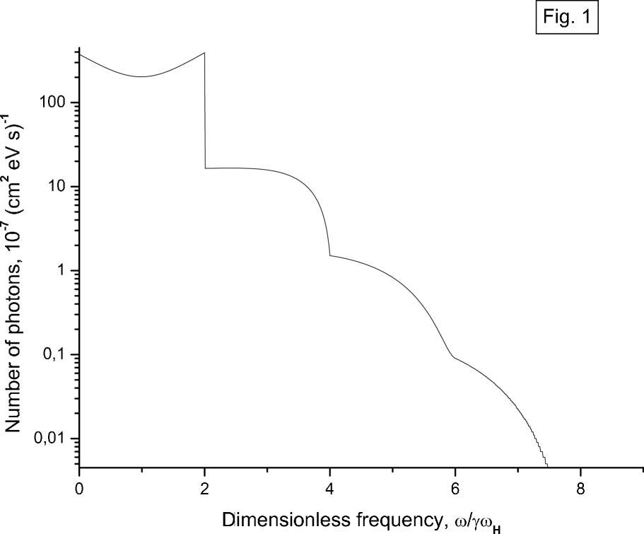
Figure 1: Spectrum of cyclotron radiation emitted by an X-ray pulsar containing four harmonics, calculated using (30). The transverse temperature of the emitting electrons is $T=20$ keV. The dimensionless frequency is plotted on a linear scale along the horizontal axis, and the number of particles on a logarithmic scale along the vertical axis.

The energy distribution of the photons that should be detected by an observer on the Earth for a transverse temperature of the emitting electrons $T=20$ keV is presented in Fig. 1. We can see that these harmonics are very broad, and overlap each other. In addition, they are clearly not equally spaced; in particular, the maximum of the second harmonic nearly coincides with the maximum of the first harmonic. The first harmonic possesses a second maximum at $\omega\simeq 0$, which is somewhat weaker than the main maximum, since higher harmonics are also added to the main maximum.

It is usual to depict the frequency dependence of the total photon energy, rather than of the number of photons. Figure 2 presents this dependence for the same transverse temperature $T=20$ keV. The formula describing this spectrum can be obtained by multiplying (30) by $\hbar\omega$. As a result, the maxima of the harmonics will be shifted; in particular, the maximum of the second harmonic will not coincide with the maximum of the first harmonic, and will appear distinct. In addition, the maximum at $\omega\simeq 0$ disappears. However, as before, the spectral features are not equidistant, and the harmonics are very broad and overlap each other.

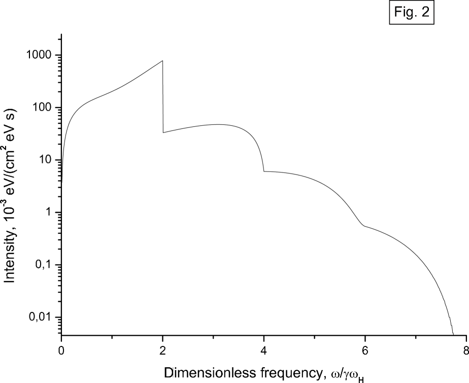
Figure 2: Energy spectrum of cyclotron radiation by an X-ray pulsar containing four harmonics. The transverse temperature of the emitting electrons is $T=20$ keV. The dimensionless frequency is plotted on a linear scale along the horizontal axis, and the number of particles on a logarithmic scale along the vertical axis.

These effects have a simple qualitative explanation. Let us consider the emission of photons in the comoving frame. First, we must answer the question of which photons will reach the distant observer. It is obvious that these will be photons movingaway from the star in the laboratory frame; i.e., those for which $\theta\leq\frac{\pi}{2}$. According to (13), this corresponds to the angles $0\leq\theta^{\prime}\leq\pi-\frac{1}{\gamma}$ ) in the comoving frame. Therefore, the observer will detect nearly all the photons, apart from those emitted precisely toward the star in the comoving frame.

As was noted above, the energy of all photons corresponding to a single harmonic is the same in the comoving frame. Nevertheless, the coefficient of transformation of the photon frequency from the comoving to the laboratory frame is not constant, and depends strongly on the angle $\theta^{\prime}$. Using (13), we can easily show that the frequency of photons emitted precisely toward the observer ($\theta^{\prime}\simeq 0$) increases by the factor $2\gamma$, the frequency of photons emitted perpendicular to the direction toward the observer ($\theta^{\prime}\simeq\pi/2$ in the comoving frame) increases by the factor $\gamma$, and the frequency of photons emitted at the angle $\theta^{\prime}=\pi-\frac{1}{\gamma}$ decreases by the factor $\gamma$. This obviously leads to considerable broadening of the lines. In addition, the equidistant character of the lines will be disrupted. This can be interpreted as follows. According to (9)), most photons associated with the first harmonic are emitted at angles $\theta^{\prime}\simeq 0$.Therefore, their frequency increases by the factor $2\gamma$, and the maximum of the first harmonic occurs at $2\gamma\omega_{H}$. On the other hand, most photons associated with the second and higher harmonics are emitted perpendicular to the direction toward the observer ($\theta^{\prime}\simeq\pi/2$), and particles with $\theta^{\prime}\simeq 0$ are virtually absent (Fig. 3). The frequencies of these photons increase only by the factor $\gamma$, so that the maxima of higher harmonics are located at

$$\omega=\gamma\omega_{n}=\gamma n\omega_{H};n>1$$ (33)

In particular, the maxima of the first and second harmonics coincide. Since the harmonics overlap, their maxima are shifted, and relation (33) is not precisely satisfied. The resulting spectrum differs substantially from a spectrum with equidistant features.

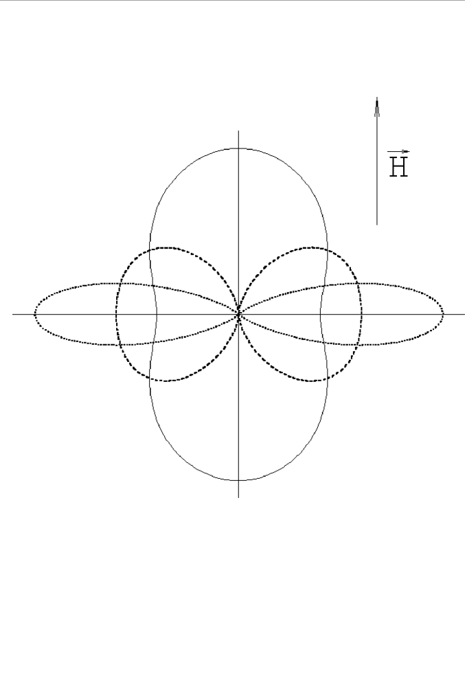
Figure 3: Diagram of the directivity of the first (solid curve), second (dashed curve), and tenth (dotted curve) cyclotron harmonics. The scales are arbitrary. The direction of the magnetic field is marked by the arrow.

We have considered above only radiation by electrons whose velocities along the field are exactly the same. At the same time, a real ensemble of electrons will certainly be characterized by some distribution of the momentum component along the field. Therefore, the total velocity distribution of the emitting electrons can be written

$$dn=f(p_{\parallel})exp\left(-\frac{m_{e}\upsilon^{2}}{2T}\right)\,dp_{\parallel}d\left(-\frac{m_{e}\upsilon^{2}}{2T}\right)$$ (34)

This distribution will considerably affect the observed spectrum of an X-ray pulsar. In particular, the first harmonic may be transformed from a sharp peak (as in Fig. 2) to a broad line. Therefore, it is interesting to answer the following question: can the distribution $f(p_{\parallel})$ in (34) be very broad for a real source, and can it result in the transformation of separate harmonics into a continuous spectrum?

As is noted above, ultrarelativistic particles can be produced by collisionless shocks formed in the accretion flow. They do not leave the shock, and oscillate at the shock front. Let us suppose that such oscillations are roughly harmonic. Then, the particle momentum will vary as $p=p_{0}\cos\alpha t$, where $\alpha$ is the oscillation frequency. Since the oscillations are ultrarelativistic, the momenta of the particles are proportional to their Lorentz factors $\gamma$ ($p\sim\gamma$), so that the $\gamma$ values vary in the same way:

$$\gamma=\gamma_{0}\cos\alpha t$$ (35)

The distribution of the corresponding ensemble of particles along the field can be represented

$$dn=\frac{N}{\pi\gamma_{0}\sqrt{1-\left(1-\frac{\gamma}{\gamma_{0}}\right)^{2}}}d\gamma;\quad\gamma\in[1;\gamma_{0}]$$ (36)

i.e., the distribution is characterized by a sharp peak with its maximum at $\gamma\simeq\gamma_{0}$. Of course, real distributions can differ considerably from (36); nevertheless, they can be sufficiently narrow that the individual cyclotron harmonics are not transformed into a continuous spectrum.

4 DISCUSSION

The parameters of the four pulsars for which higher cyclotron harmonics have been detected are presented in the table. Let us consider in more detail the high-energy spectra of these sources, since they contain the features of the most interest to us. The spectrum in this region possesses a quasi-power-law character with an exponential cut-off (if cyclotron features are not taken into consideration), as is very typical for X-ray pulsars. Spectra of this form are supposed to be produced by comptonization of relatively cool radiation by hot electrons, considered in detail [14]. The resultingspec trum for energies above the cut-off at $E_{c}$ is approximately a Wien spectrum with the characteristic temperature equal to the temperature of the hot electrons $T_{e}$ [15]. It is formed by photons that have undergone a large number of collisions with the electrons, and have therefore been heated to the temperature $T_{e}$. On the other hand, the photons forming the power-law part of the spectrum have experienced only a few collisions with hot electrons, and have not reached thermal equilibrium. As a result, the power-law spectrum at each specific frequency contains fewer photons than a Planck spectrum with temperature $T_{e}$.

To form an absorption line in such a spectrum, the electrons must have a temperature below $T_{e}$. Even if we assume that the electron-velocity distribution differs considerably from maxwellian, the situation is unlikely to change fundamentally. In any case, the characteristic energy of motion of the electrons across the magnetic field should not exceed $T_{e}$. The table shows that, for all four sources, the temperature $T_{e}$ does not exceed $20$ keV. On the other hand, the temperature of the electrons forming complex cyclotron lines must be considerably greater: for either emission or absorption harmonics of higher orders to appear in the spectrum, the velocity of the electrons across the magnetic field must be comparable to the speed of light; i.e., their temperature must be comparable to $mc^{2}\simeq 500$ keV. This requirement can be explained quantitatively. The ratio of the optical depths of the ultrarelativistic electrons to cyclotron emission (or absorption) at two neighboring harmonics is of the order of the ratio of the mean kinetic energy of motion of the particles across the magnetic field to their rest energy. We can easily demonstrate using(9) that, if the motion of the electrons across the field is slow ($\upsilon\ll c$), this ratio is

$$\frac{\tau_{n+1}}{\tau_{n}}=\frac{n(n+2)}{n+\frac{3}{2}}\left(1+\frac{1}{n}\right)^{2n+2}\left(\frac{kT}{2m_{e}c^{2}}\right)$$ (37)

Consequently, if the temperature satisfies the condition

$$T<T_{e}\sim 20\mbox{keV}$$ (38)

then the intensity of harmonics should decrease rapidly with increasing harmonic number. In particular, the optical-depth ratio for the second and first harmonics should not exceed $\frac{2}{5}$. However, observed values of this ratio (presented in the table) are $2.7$ for X0115+63, $9.3$ for 4U1907+09, $>1.8$ for Vela X-1, and $2.8$ for A0535+26 (the cyclotron features were considered in all cases to be absorption features). According to (37), this corresponds to electron temperatures of $141$, $483$, $94$, and $146$ keV, respectively. It is unclear how these hot electrons can absorb radiation with a temperature of $\sim 20$ keV. Consequently, the cyclotron features observed in the spectra of these objects must be emission lines.

Source	X0115+63	Vela X-1	4U1907+09	A0535+26
Reference	[10]	[3]	[5]	[22]
Temperature
of the Planck	17,4	9,4	12	18,7
tail $T_{e}$(keV)
Ratio
of optical depths	2,7	1,8 - 9,8	9,3	2,8
of the first and second
harmonics $\tau_{2}/\tau_{1}$

As was reported in [9] and [3] the cyclotron lines in the spectra of X0115+63 and Vela X-1 are not equally spaced (the lines were considered in both papers to be absorption features). Let us discuss X0115+63 in more detail. The observed lines in its spectrum [10] are not equidistant (if they are considered to be emission features). In addition, the lines are very broad and overlapping. All these characteristic features of the cyclotron spectrum are usually explained by the complex geometry of the emitting region (a hot spot on the surface of the neutron star). The broadening of the line and its transformation to a broad band are thought to be due to variations in the intensity of the magnetic field within the emitting region, while the higher harmonics are formed in parts of the hot spot where the magnetic field is weaker than in the regions of formation of the main harmonic, so that their frequencies are shifted with respect to the fundamental frequency, $\omega_{n}<n\omega_{1}$.

Unfortunately, this explanation runs into serious problems. It is not difficult to estimate the relative broadening of lines due to the above mechanism. First, we have

$$\frac{\Delta\omega}{\omega}=\frac{\Delta H}{H}$$ (39)

Let us assume that a neutron star is characterized by the standard radius ($R=10~{}{}$) and mass ($M=1.4M_{\odot}$), a dipolar magnetic field

$$H_{r}=\frac{\bf m}{r^{3}}\cos\theta;\qquad H_{\theta}=-\frac{\bf m}{2r^{3}}\sin\theta;$$ (40)

and a temperature at the foot of the accretion column $T_{e}\sim 10$ keV. Then, the height of the hot region is approximately determined by the usual barometric formula

$$\Delta r=\frac{kT_{e}}{m_{H}g}$$

where $k$ is the Boltzmann constant, $m_{H}$ the mass of the hydrogen atom (the dominant component of the accretion gas), and $g$ the free-fall acceleration at the neutron-star surface. Substituting the numerical values, we obtain $\Delta r\sim 0.7~{}{}$. The relative variation in the magnetic field of the form (40) within this distance from the neutron-star surface is

$$\frac{\Delta H}{H}=3\frac{\Delta r}{R}\sim 2\cdot 10^{-4}$$

Consequently, $\displaystyle{\frac{\Delta\omega}{\omega}\sim 2\cdot 10^{-4}}$. Further, let us estimate the variations in the magnetic field over the spot. If the angular scale of the spot is $\chi$, then, as obviously follows from (40), the corresponding relative variation in the magnetic field will be

$$\frac{\Delta H}{H}=\frac{3}{8}\chi^{2}$$

According to [17], the angular size of the spot is

$$\chi\simeq\sin\chi=7,455\cdot 10^{-4}H^{-\frac{2}{7}}L^{\frac{1}{7}}$$

where $L$ is the luminosity of the X-ray pulsar. The luminosity of the pulsar X0115+63 is $L\simeq 10^{37}$ erg/s [2], while the magnetic field (derived from the energy of the cyclotron line using the nonrelativistic formula) would be at least $7\cdot 10^{11}$ Gs. Hence, $\chi\simeq 0,06$, i.e. $\displaystyle{\frac{\Delta\omega}{\omega}=\frac{\Delta H}{H}\approx 1,4\cdot 10^{-3}}$.

Therefore, the possible broadening or shift of the cyclotron line frequency due to the source geometry is $\displaystyle{\frac{\Delta\omega}{\omega}\leq 2\cdot 10^{-3}}$. Of course, this is completely inadequate to explain the observed width of the lines ($\displaystyle{\frac{\Delta\omega}{\omega}\sim 0.2}$), Moreover, to reproduce the non-equal spacing of the lines, it is necessary to suppose a complex (and, therefore, quite artificial) temperature distribution over the spot. Thus, we cannot explain the observed width of the cyclotron lines, their deviation from an equidistant distribution, or their overlapping using only geometrical considerations. The most probable and natural explanation of all these properties is that the electrons giving rise to the cyclotron lines are ultrarelativistic, and so have a very anisotropic distribution of the form (34). Radiation produced by such particles possesses precisely these features. Therefore, the presence of several broad cyclotron lines separated by unequal distances in an X-ray pulsar s spectrum represents a strong argument in favor of our mechanism for the formation of the cyclotron features. The spectrum of cyclotron radiation calculated using( (28). is plotted in Fig. 4 on a log log scale for a transverse temperature of 20 keV. There is an obvious similarity between the observed spectrum of X0115+63 in [10] and the calculated spectrum in Fig. 4. Although the first harmonic in Fig. 4 represents a sharp peak, whereas it is quite broad in the observed spectrum, this could be explained as an effect of the velocity distribution (34) of the emitting electrons along the magnetic field. This same distribution should also result in additional broadening of the cyclotron lines.

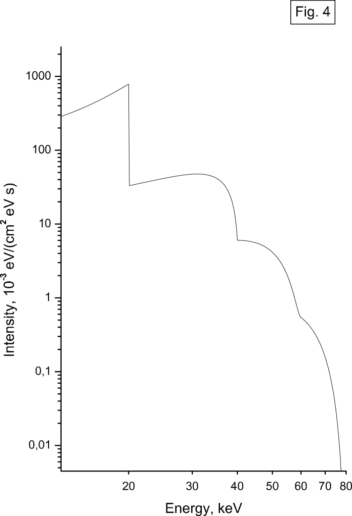
Figure 4: Energy spectrum of cyclotron radiation by an X-ray pulsar containing four harmonics. The transverse temperature of the emitting electrons is $T=20$ keV. The scales are logarithmic along both axes.

The calculated cyclotron spectrum displays another very interesting feature: as we can see in Fig. 2, the dips between neighboring harmonics are located at nearly equal distances from each other. Therefore, if these decreases in intensity in the observed spectrum were interpreted as absorption lines, they would appear be equidistant. This is probably why the cyclotron features in the spectra of X0115+63, Vela X-1, 4U1907+09, and A0535+26 have been interpreted as a set of equidistant absorption lines. However, as is demonstrated above, they are more likely to be emission rather than absorption lines.

We have already noted that ultrarelativistic, anisotropic electrons can be produced by a collisionless shock in the accretion flow. As is shown in [15, 16] such shocks can indeed form, and the corresponding electrons will have a strongly anisotropic velocity distribution. This is due to the fact that the electrons are accelerated primarily along the magnetic field. In addition, the transverse component of their momenta rapidly decreases due to radiative cooling, while the component along the field changes relatively little. The estimation of the electron temperature performed in [15, 16] yielded values $T\sim 10$ MeV, corresponding to $\gamma\sim 20$, i.e. the electrons are ultrarelativistic.

Note also that there is considerable indirect evidence that the particles forming the cyclotron lines in the spectra of X-ray pulsars are ultrarelativistic, primarily associated with discrepancies in estimates of the magnetic fields of these objects [11].

The pulsar Her X-1 was considered in detail in [17]. In general, its rotation speeds up, but it experiences deceleration in some intervals [18]. Consequently, its period is close to the equilibrium period; i.e., the angular velocity of rotation of the neutron star together with its magnetosphere is close to keplerian at the Alfven radius. We can use this fact to estimate the magnetic field of this pulsar, which turns out to be relatively small, about $H=3\cdot 10^{11}$ Gs. In addition, radio pulsars in binary systems possess anomalously weak magnetic fields, $H\simeq 10^{8}-10^{11}$ Gs [19]. Their formation as the result of the evolution of a pair containing an X-ray pulsar could be naturally explained if these pulsars had comparatively small magnetic fields, $H<3\cdot 10^{11}$ Gs. Mihara et al. [20] explained the observed 35-day cycle of Her X-1 as the result of periodic eclipses of the emitting region on the neutron star surface by the accretion disk. For this mechanism to operate, the disk must be located at a sufficiently short distance from the surface; i.e., the field must be $H<10^{11}$ Gs.

At the same time, a cyclotron line at energy $3556$ keV is observed in the spectrum of Her X- 1. If the nonrelativistic formula (2), is applied, this corresponds to a magnetic field of $(3-5)\cdot 10^{12}$ Gs. This contradiction appears to be due to the fact that the electrons emitting the cyclotron line are actually ultrarelativistic. In this case, as is shown above, the energy of the first (fundamental) harmonic increases by the factor $2\gamma$. Therefore, the nonrelativistic formula gives a substantially (by a factor of $2\gamma$) overestimated value for the magnetic field. Thus, adopting the hypothesis that the velocities of the electrons emitting the cyclotron line are ultrarelativistic along the field makes it possible to avoid contradictions between estimates of the pulsar s magnetic field given by various methods; this represents weighty indirect evidence in favor of our mechanism for the formation of the cyclotron radiation.

Another argument supporting this mechanism is the observation of correlated variations in the energies of the cyclotron lines of some pulsars and in their luminosities [21]. This correlation can be explain in a natural way by our model. The luminosity of the hot spot is comparable to the Eddington luminosity; i.e., the radiation pressure appreciably affects the accretion rate. If the luminosity increases, the accretion flow will be substantially slowed. As a result, the intensity of the shock decreases, and the mean energy of the ultrarelativistic particles produced by the shock decreases. Consequently, the energy of the cyclotron lines also decreases [11]. However, we emphasize that it is recent observations of higher harmonics and their deviations from an equidistant spectral distribution that represent the first direct evidence that the electrons emitting the cyclotron lines are ultrarelativistic, and have very anisotropic distributions of the form (34).

In this mechanism for the formation of the cyclotron lines, we must know the electron Lorentz factor $\gamma$ to determine the pulsar s magnetic field. In turn, this factor depends on the physical conditions in the accretion flow, in particular, in the collisionless shocks. It is possible that different types of X-ray pulsars have different shock structures, and, therefore, different characteristic $\gamma$ values.

Accretion in low-mass binary systems occurs via the flow of material through the inner Lagrange point when the donor star fills its Roche lobe, whereas accretion in massive systems occurs via the capture of material from the powerful stellar wind of the O B companion, which does not fill its Roche lobe. It may not be a chance coincidence that all four sources displaying several cyclotron harmonics are associated with massive systems, so that the second type of accretion is realized. In this case, the conditions at the front of the collisionless shock may be more favorable for the ultrarelativistic electrons to acquire greater momentum transverse to the magnetic field, resulting in the appearance of higher cyclotron harmonics in the pulsar spectrum.

5 CONCLUSION

The presence of several cyclotron harmonics in the spectra of X-ray pulsars provides important information about their physical properties.

First, the cyclotron features should apparently not be interpreted as absorption lines. The ratio of the optical depths of harmonics of different orders can be used to estimate the temperature of the electrons participating in the formation of the cyclotron features. For absorption to take place, this temperature must be less than the temperature of the Planck tail that is often observed in the spectra of X-ray pulsars. As a rule, $T_{e}$ is not large: for many pulsars, $T_{e}<20~{}{KeV}$. As a result, the second harmonic is substantially weaker than the first, and is difficult to detect observationally. In any case, the cyclotron features in all four sources for which the second harmonic has been observed are very likely emission features.

Second, if the cyclotron emission lines are not equidistant, this argues strongly that the electrons emitting these lines are ultrarelativistic and have a very anisotropic distribution. Emission by such electrons displays characteristic properties that are not typical of emission by nonrelativistic particles, and which are actually observed in the observed spectra of X-ray pulsars. There is also other (indirect) evidence supporting this mechanism for the cyclotron-line formation. Thus, the cyclotron radiation of X-ray pulsars is most likely produced by anisotropic ultrarelativistic electrons. As a result, the nonrelativistic formula (2) considerably overestimates the pulsar magnetic fields. The magnitude of this overestimation depends on the distribution function (34) of the emitting electrons in the corresponding shocks. We cannot rule out the possibility that this function may be different for different types of X-ray pulsars. Subsequent studies of the physical processes occurring in the accretion flows of these objects may help shed light on this problem.

Thus, investigations of the spectra of X-ray pulsars containing several cyclotron harmonics may enable us to refine estimates of their magnetic fields, and thereby to resolve questions concerning the structure and evolution of these objects.

6 ACKNOWLEDGEMENTS

I am grateful to G.S. Bisnovatyi-Kogan for help in preparation of this article and, in particular, for several fruitful ideas. This work was supported by the Russian Foundation for Basic Research (project codes 01-02-06146 and 99-02-18180).

References

- [1] Trümper, J., Pietsch, W., Reppin, C. et al. // Ap.J.(letters), 1978, V. 219, L. 105.
- [2] White, N. E., Swank, J. H., Holt, S. S. // Ap.J., 1983, V. 270, p. 711.
- [3] Kreykenbohm, I., Kretschmar, P., Wilms, J., et al. // 1998, A&A, V.341, p. 141.
- [4] Orlandini, M., et al. // 1998, A&A, V.332, p. 121.
- [5] Cusumano, G., Di Salvo, T., Orlandini, M., Piraino, S., Robba, N., Santangelo, A. // 1998, A&A, V. 338, L. 79.
- [6] Santangelo, A., et al. // 1999, Proc. Taomina Integral Workshop.
- [7] Kendziorra, E., Kretschmar, P., Pan H.C., Kunz, M., et al. // 1994, A&A, V. 291, L. 31.
- [8] Iwasawa, K., Koyama, K., Halpern, J. // 1992, PASJ, V. 44, p. 9.
- [9] Heindl, W.A., Coburn, W., Gruber, D.E., et al. // 1999, Ap.J.(Letters), V. 521, L. 49.
- [10] Santangelo, A., Segreto, A., Giarrusso, S. et al. // Ap.J.(Letters), 1999, V. 523, L. 85.
- [11] A. N. Baushev and G. S. Bisnovatyi-Kogan // Astron. Zh. 76, 283 (1999) [Astron. Rep. 43, 241 (1999)].
- [12] Landau, L.D., Lifshitz, E.M. // The Classical Theory of Fields, any edition.
- [13] V. L. Ginzburg // Theoretical Physics and Astrophysics (Nauka, Moscow, 1975; Pergamon, Oxford, 1979).
- [14] Sunyaev, R.A., Titarchuk, L.G. // Astron.Ap. , 1980, V. 86, p. 121.
- [15] Ya. B. Zeldovich and N. I. Shakura // Astron. Zh. 46, 225 (1969) [Sov. Astron. 13, 175 (1969)].
- [16] G. S. Bisnovaty..-Kogan and A. M. Fridman // Astron. Zh. 46, 721 (1969) [Sov. Astron. 13, 566 (1969)].
- [17] G. S. Bisnovatyi-Kogan // Byull. Akad. Nauk Gruz. SSR, Abastumanskaya Astrofiz. Obs. 58, 175 (1985).
- [18] V. M. Lipunov // Astron. Zh. 64, 321 (1987) [Sov. Astron. 31, 167 (1987)].
- [19] Boriakoff, V., Buecheri, R., Fauci, F. // Nature, 1983 , V. 304, p. 417.
- [20] E. K. Sheffer, I. F. Kopaeva, et al. // Astron. Zh. 69, 82 (1992) [Sov. Astron. 36, 41 (1992)].
- [21] Mihara, T., Makishima, K., Nagase, F. // Proceedings of an international Workshop ”All-sky X-ray Observations in the Next Decade” 1997, March 3-5, p. 135.
- [22] V. V. Borkus, A. S. Kaniovsky, R. A. Sunyaev, et al. // Pis ma Astron. Zh. (1998), 24, 415 [Astron. Lett. (1998), 24, 350].