Nilpotent noncommutativity and renormalization

Abstract

We analyze renormalizability properties of noncommutative (NC) theories with a bifermionic NC parameter. We introduce a new 4-dimensional scalar field model which is renormalizable at all orders of the loop expansion. We show that this model has an infrared stable fixed point (at the one-loop level). We check that the NC QED (which is one-loop renormalizable with usual NC parameter) remains renormalizable when the NC parameter is bifermionic, at least to the extent of one-loop diagrams with external photon legs. Our general conclusion is that bifermionic noncommutativity improves renormalizablility properties of NC theories.

1 Introduction

It is well known [1] that noncommutative (NC) field theories have renormalizability problems due to the so-called UV/IR mixing [2, 3, 4]. To overcome this difficulty, one modifies the propagator by adding an oscillator term [5, 6, 7] in order to respect the Langmann-Szabo duality [8], or by adding a term with a negative power of the momentum [9]. Supersymmetry also improves the renormalizability properties of NC theories (see, e.g., [10]). Some versions of NC supersymmetry (those which are based on the nonanticommutative superspace [11, 12], see also [13, 14]) have a nilpotent NC parameter, so that the star product terminates at a finite order of its expansion. It was demonstrated [15] that having a nilpotent NC parameter does not necessarily imply supersymmetry. In [15] a nilpotent (bifermionic) NC parameter was introduced in a bosonic theory, giving rise to many attractive properties of that model. The aim of this work is to study to which extent having a nilpotent (or bifermionic) NC parameter influences the renormalization. We shall consider non-supersymmetric theories in order to separate the effects of nilpotency from the effects of supersymmetry.

A suitable framework for such an analysis was suggested in [15], where it was proposed to consider a bifermionic NC parameter

$$\Theta^{\mu\nu}=i\theta^{\mu}\theta^{\nu},$$ (1)

where $\theta^{\mu}$ is a real constant fermion (a Grassmann odd constant), $\theta^{\mu}\theta^{\nu}=-\theta^{\nu}\theta^{\mu}$. Note that bifermionic constants appear naturally in pseudoclassical models of relativistic particles [16, 17]. Due to the anticommutativity of $\theta^{\mu}$, the expansion of the usual Moyal product terminates at the second term,

$$f_{1}\star f_{2}=\exp\left(\frac{i}{2}\Theta^{\mu\nu}\partial_{\mu}^{x}\partial_{\nu}^{y}\right)f_{1}(x)f_{2}(y)|_{y=x}=f_{1}\cdot f_{2}-\frac{1}{2}\theta^{\mu}\theta^{\nu}\partial_{\mu}f_{1}\partial_{\nu}f_{2}.$$ (2)

The star-product, therefore, becomes local.

In [15] a bifermionic NC parameter was used to construct a two-dimensional field theory model which, in contrast to usual time-space NC models, has a locally conserved energy momentum tensor, a well-defined conserved Hamiltonian, and can be canonically quantized without any difficulties. Besides, the model appears to be renormalizable. In the present work we study whether bifermionic noncommutativity helps renormalize theories in four dimensions.

First we explore a model which is a four-dimensional version of the model suggested in [15] (this is nothing else than NC $\varphi^{4}$ with an additional interaction included to make it less trivial). We find that for a bifermionic NC parameter this model becomes renormalizable at all orders of the loop expansion. We also study the one-loop renormalization group equations and find an infrared stable fixed point where all couplings vanish.

From the technical point of view, having a bifermionic NC parameter looks similar to expanding the theory in $\Theta$ and keeping just a few leading terms. The ultraviolet properties of the expanded and full theories are rather different, and, sometimes, expanded theories behave worse (see, e.g., [19]). The reason is that, on one hand, the propagator in expanded theories does not have an oscillatory behavior, and, on the other hand, dangerous momentum-dependent vertices appear. All these problems appear also in theories with bifermionic noncommutativity, but there is also an effect which improves the ultraviolet behavior. Namely, some divergent terms vanish due to $\theta^{2}=0$. Here we take the NC QED (which is one-loop renormalizable if the standard NC parameter is used) and demonstrate that with a bifermionic NC parameter this model remains renormalizable at least for one loop diagrams with external photons.

2 A scalar field model

The action of the model we consider in this section reads

$$S=\int d^{4}x\left(\frac{1}{2}(\partial_{\mu}\varphi_{1})^{2}+\frac{1}{2}(\partial_{\mu}\varphi_{2})^{2}+\frac{1}{2}(\partial_{\mu}\varphi)^{2}-\frac{1}{2}m_{1}^{2}\varphi_{1}^{2}-\frac{1}{2}m_{2}^{2}\varphi_{2}^{2}-\frac{1}{2}m^{2}\varphi^{2}\right.$$

$$\qquad\qquad\left.-\frac{ei}{2}[\varphi_{1},\varphi_{2}]_{\star}\star\varphi\star\varphi-\frac{\lambda}{24}\varphi_{\star}^{4}\right),$$ (3)

which is a four dimensional version of a model suggested in [15]. The motivations for taking this particular form of the model are as follows. Since any symmetrized star product with a bifermionic parameter is equivalent to the usual commutative pointwise product, we need at least two fields, $\varphi_{1}$ and $\varphi_{2}$, to construct a non-trivial polynomial interaction term. As was explained in [15], even two fields are not enough, so we take another scalar field $\varphi$ to construct the interaction term with a coupling constant $e$. We also added a self-interaction term $\varphi_{\star}^{4}=\varphi\star\varphi\star\varphi\star\varphi$ to make the dynamics more interesting. $e$ and $\lambda$ are real coupling constants.

In [15] it was demonstrated that a two dimensional model with the same Lagrange density as in (3) is renormalizable. It is relatively easy to achieve renormalizability in two dimensions. For example, there is a model of NC gravity in two dimensions for which the entire quantum generating functional of Green functions can be calculated non-perturbatively at all orders of the loop expansion [20] by using methods developed earlier in the commutative case [21]. Here, to be closer to physics, we consider a four-dimensional model (3).

Due to our choice (1) of the NC parameter, the interaction part of the action (3) looks rather simple,

$$S_{{\rm int}}=\int d^{4}x\left(\frac{ei}{2}(\theta^{\mu}\partial_{\mu}\varphi_{1})(\theta^{\nu}\partial_{\nu}\varphi_{2})\varphi^{2}-\frac{\lambda}{24}\varphi^{4}\right).$$ (4)

Now we are ready to derive the Feynman rules for our model. The propagators are the standard propagators of massive scalar fields. There are two vertices, the standard $\varphi^{4}$ vertex and a new vertex, which depends on the NC parameter.

            

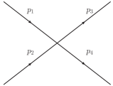
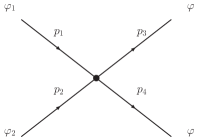
Figure 1: The standard $\varphi^{4}$ vertex and the new vertex $-\frac{ie}{2}\theta p_{1}\theta p_{2}$.

The main observation which proves the renormalizability of (3) is that any diagram with an internal line of either $\varphi_{1}$ or $\varphi_{2}$ field vanishes. Indeed, any internal line of these fields inevitably connects two "new" vertices and, therefore, receives a multiplier $(\theta\cdot k)^{2}=0$, where $k$ is the corresponding momentum. Power-counting renormalizability of our model follows then by standard arguments, precisely as in the commutative case. Consider a diagram with $N$ vertices and $2K$ external legs. This diagram has $\frac{1}{2}(4N-2K)=2N-K$ internal lines, giving the total power of the momenta in the integrand $-2(2N-K)$. The momenta of the internal lines are restricted by $N-1$ delta-functions, where $-1$ corresponds to conservation of the total momenta of all external legs. Putting all this together, we obtain that the degree of divergence is $4-2K$, as in the commutative $\varphi^{4}$ theory. The power-counting divergent diagrams are the ones with $2$ or $4$ external legs. The diagrams containing $\varphi$ legs only are precisely the same as in the commutative case, and they are renormalized in precisely the same way. Let us consider the diagrams with $\varphi_{1}$ and $\varphi_{2}$ legs. There are three types of such diagrams (see Fig. 2)

                  

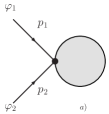
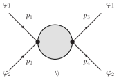
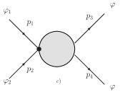
Figure 2: The three divergent diagrams.

The diagram on Fig. 2a is proportional to $(p\theta)^{2}$, and, therefore, vanishes. The diagram on Fig. 2b contains $(p_{1}\theta)(p_{2}\theta)(p_{3}\theta)(p_{4}\theta)=0$, due to momentum conservation, $p_{1}+p_{2}=p_{3}+p_{4}$. The diagram of Fig. 2c is at most logarithmically divergent. Therefore, their divergent parts are proportional to the lowest power of the external momenta, i.e., to $(p_{1}\theta)(p_{2}\theta)$. It is easy to see, that such divergences can be removed by a renormalization of the coupling $e$ in the action (3). We conclude that the model (3) with a bifermionic NC parameter is renormalizable at all orders of the loop expansion.

The renormalization of all parameters related to the field $\varphi$ (the renormalization of $m$, $\lambda$ and of the wave function $\varphi$) is not sensitive to the presence of the other fields $\varphi_{1}$ and $\varphi_{2}$. There is no renormalization of the mass or of the wave function $\varphi_{1}$ or $\varphi_{2}$. By comparing combinatoric factors appearing in front of the relevant Feynman diagrams, and using the standard result [18] for commutative $\varphi^{4}$ theory in the dimensional regularization scheme, one can derive a relation

$$3\frac{\delta e}{e}=\frac{\delta\lambda}{\lambda}=\frac{\lambda}{16\pi^{2}}\frac{3}{\epsilon}$$ (5)

between infinite one-loop renormalizations of the charges $e$ and $\lambda$. The $\beta$-function for $\lambda$ is well known [18]

$$\beta_{\lambda}=-\epsilon\lambda+\frac{3\lambda^{2}}{16\pi^{2}}+O(\lambda^{3}).$$ (6)

From the relation (5) one can obtain the anomalous dimension of the coupling $e$, $\beta_{e}$, using the fact that the bare coupling is renormalization-group invariant,

$$\mu\frac{de_{0}}{d\mu}=0\,,\,\,e_{0}=\mu^{\epsilon}e\left(1+\frac{\lambda}{16\pi^{2}}\frac{1}{\epsilon}\right)\,.$$

Explicitly,

$$\mu\frac{d}{d\mu}e_{0} = \mu^{\epsilon}\left(\epsilon e+\frac{e\lambda}{16\pi^{2}}\right)+\mu^{\epsilon}\left[\beta_{e}\left(1+\frac{\lambda}{16\pi^{2}}\frac{1}{\epsilon}\right)+\frac{e}{16\pi^{2}}\frac{1}{\epsilon}\beta_{\lambda}\right]=0\,,$$

which implies

$$\beta_{e} = -\left[\epsilon e+\frac{e\lambda}{16\pi^{2}}+\frac{e}{16\pi^{2}}\frac{1}{\epsilon}\beta_{\lambda}\right]\left(1-\frac{\lambda}{16\pi^{2}}\frac{1}{\epsilon}\right)$$

$$= -\epsilon e+\frac{\lambda e}{16\pi^{2}}+O\left(e\lambda^{2}\right).$$

Now we can remove the regularization by setting $\epsilon=0$ and solve the renormalization group equations

$$\mu\frac{d}{d\mu}\lambda(\mu)=\beta_{\lambda}(\lambda(\mu)),\qquad\mu\frac{d}{d\mu}e(\mu)=\beta_{e}(e(\mu))$$ (7)

for the running couplings $\lambda(\mu)$ and $e(\mu)$. The initial conditions are $\lambda(\mu_{0})=\lambda$, $e(\mu_{0})=e$ with $\mu_{0}$ being a normalization scale. Since $\beta_{\lambda}$ does not depend on $e$, the equation for $\lambda(\mu)$ may be solved first, giving the well-known result

$$\lambda\left(\mu\right)=\lambda\left(1-\frac{3}{16\pi^{2}}\lambda\ln\frac{\mu}{\mu_{0}}\right)^{-1}.$$ (8)

Solving then the equation for $e(\mu)$ we obtain

$$e\left(\mu\right)=e\left(1-\frac{3\lambda}{16\pi^{2}}\ln\frac{\mu}{\mu_{0}}\right)^{-\frac{1}{3}}.$$ (9)

In the limit $\mu\to 0$ both couplings vanish, and we have an infrared stable fixed point. Note, that $e(\mu)$ vanishes slower than $\lambda(\mu)$ while approaching the fixed point.

3 Noncommutative QED with bifermionic parameter

Let us consider NC QED in Euclidean space with the classical action

$$S_{cl}=\int d^{4}x\left[\frac{1}{4g^{2}}\hat{F}_{\mu\nu}^{2}+\bar{\psi}\left(i\gamma_{\mu}D_{\mu}\right)\psi\right]$$ (10)

where $D_{\mu}\psi=\partial_{\mu}\psi-iA_{\mu}\star\psi$ and

$$\hat{F}_{\mu\nu}=F_{\mu\nu}-i(A_{\mu}\star A_{\nu}-A_{\nu}\star A_{\mu}),\qquad F_{\mu\nu}=\partial_{\mu}A_{\nu}-\partial_{\nu}A_{\mu}\,.$$

The $\gamma$-matrices satisfy $\left\{\gamma_{\mu},\gamma_{\nu}\right\}=2\delta_{\mu\nu}$ and are hermitian, $\delta_{\mu\nu}=\mathrm{diag}\left(1,1,1,1\right)$. For ordinary NC parameter, this theory is known to be one-loop renormalizable [22, 23]. But an expansion in $\Theta$ can violate renormalizability already at one loop, as was demonstrated in [19] in the framework of the Seiberg-Witten map.

Here we check whether NC QED remains renormalizable at one loop if the NC parameter is bifermionic (1). To simplify our analysis we consider the case when only $\psi$ is quantized while $A_{\mu}$ remains a classical background field. One can check that this corresponds to retaining all diagrams with external photons in the Lorentz gauge. Renormalizability in such a simplified model means that the one-loop divergence is proportional to the corresponding term in the classical action (10), namely, to $\hat{F}_{\mu\nu}^{2}$. The effective action can be formally written as

$$W=-\ln\det\not{D}=-\frac{1}{2}\ln\det\not{D}^{2}$$ (11)

where $\not{D}$ is the Dirac operator on noncommutative $\mathbb{R}^{4}$ in the presence of an external electromagnetic field.

$$\not{D}=i\gamma_{\mu}\left(\partial_{\mu}-iA_{\mu}\star\right)=i\gamma_{\mu}\left(\partial_{\mu}-iA_{\mu}+\frac{i}{2}\theta\partial A_{\mu}\theta\partial\right)\,,\,\,\theta\partial\equiv\theta_{\mu}\partial_{\mu}\,.$$ (12)

To avoid writing too many brackets we adopt the convention that the derivative only acts on the function which is next to it on the right (ignoring, of course, any number of $\theta$’s or other derivatives which may appear in between). For example, $\theta\partial A_{\mu}\theta\partial=(\theta\partial A_{\mu})\theta\partial$ is a first-order differential operator.

It is convenient to use the zeta-function regularization of functional determinants [24, 25], so that the regularized effective action (11) reads $W^{{\rm reg}}=\frac{1}{2}\zeta(\not{D}^{2},s)\Gamma(s)$ where $\zeta(\not{D}^{2},s)={\rm Tr}_{L^{2}}((\not{D}^{2})^{-s})$. In the physical limit, $s\to 0$, the regularized effective action diverges, and the divergent part reads

$$W^{{\rm div}}=\frac{1}{2s}\zeta(\not{D}^{2},0).$$ (13)

Usually, $\not{D}^{2}$ is an operator of Laplace type, so that the heat trace

$$K(\not{D}^{2};t)={\rm Tr}_{L^{2}}(e^{-t\not{D}^{2}})$$ (14)

exists and admits an asymptotic expansion

$$K(\not{D}^{2};t)\simeq\sum_{k\geq 0}t^{\left(k-n\right)/2}a_{k}\left(\not{D}^{2}\right)$$ (15)

as $t\to+0$. Here $n$ the is dimension of the underlying manifold. A review of the heat kernel expansion can be found in [26] for commutative manifolds, and in [27] for the NC case. Let us assume that the expansion (15) is valid for the operator (12). (This will be demonstrated in a moment). Then, by using the Mellin transform, one can show

$$\zeta(\not{D}^{2},0)=a_{4}(\not{D}^{2})$$ (16)

in $n=4$ dimensions. There is no good spectral theory for differential operators with symbols depending on fermionic parameters. To be on the safe side, we shall evaluate (16) by two independent methods.

First, we use existing results on the heat kernel expansion on NC manifolds. The operator

$$\not{D}^{2}=-\left((\partial_{\mu}-iA_{\mu}\star)^{2}-\frac{i}{4}[\gamma^{\mu},\gamma^{\nu}]\hat{F}_{\mu\nu}\star\right),$$ (17)

(where partial derivatives act all the way to the right), has left star-multiplications only (meaning that in the eigenvalue equation $\not{D}^{2}\psi=\lambda\psi$ all background fields multiply $\psi$ from the left), and, therefore, falls into the category considered in [28, 29]. The calculations made in [28] are regular at $\Theta=0$ and survive an expansion to a finite order in $\Theta$ (see eqs.(15) - (26) there). Note that such a statement is not true for operators having both right and left star multiplications [30, 31]. Anyway, we are allowed to use the results of [28, 29] for the operator (17). First, we bring $\not{D}^{2}$ to the standard form

$$\not{D}^{2}=-\left(\hat{\nabla}_{\mu}\hat{\nabla}_{\mu}+\hat{E}\star\right),\qquad\hat{\nabla}_{\mu}\equiv\partial_{\mu}+\hat{\omega}_{\mu}\star\,,$$ (18)

where

$$\hat{\omega}_{\mu}=-iA_{\mu},\qquad\hat{E}=-\frac{i}{4}[\gamma^{\mu},\gamma^{\nu}]\hat{F}_{\mu\nu}.$$ (19)

Then, according to [28, 29], the asymptotic expansion (15) exists and the coefficient $a_{4}$ reads

$$a_{4}=\frac{1}{(4\pi)^{2}}\,\frac{1}{12}\int d^{4}x\,{\rm tr}\,(6\hat{E}\star\hat{E}+\hat{\Omega}_{\mu\nu}\star\hat{\Omega}_{\mu\nu})$$ (20)

with $\hat{\Omega}_{\mu\nu}=[\hat{\nabla}_{\mu},\hat{\nabla}_{\nu}]$. By substituting (19) in (20) and taking the trace, we obtain

$$a_{4}(\not{D}^{2})=\frac{1}{\left(4\pi\right)^{2}}\frac{2}{3}\int d^{4}x\hat{F}_{\mu\nu}\star\hat{F}_{\mu\nu}\,.$$ (21)

The other method we use does not rely on the star-product structure, but rather uses an expanded form of the operator

$$\not{D}^{2}=-(\partial^{2}-2iA_{\mu}\partial_{\mu}-i(\partial_{\mu}A_{\mu})-A^{2})-i\left(\theta\partial\right)A^{\mu}\left(\theta\partial\right)\partial_{\mu}$$

$$\qquad-\frac{i}{8}\left[\gamma^{\mu},\gamma^{\nu}\right]\left(\theta\partial\right)F_{\mu\nu}\left(\theta\partial\right)-\frac{i}{2}\left(\theta\partial\right)\partial^{\mu}A_{\mu}\left(\theta\partial\right)-A^{\mu}\left(\theta\partial\right)A_{\mu}\left(\theta\partial\right)$$

$$\qquad-\frac{1}{4}\left[\gamma^{\mu},\gamma^{\nu}\right]\left(\theta\partial\right)A_{\mu}\left(\theta\partial\right)A_{\nu}+\frac{i}{4}\left[\gamma^{\mu},\gamma^{\nu}\right]F_{\mu\nu}\,.$$ (22)

The coefficient $a_{4}$ can be read off from the seminal paper by Gilkey [32] by identifying corresponding invariants. For any Laplace type operator of the form

$$P=-\left(g^{\mu\nu}\partial_{\mu}\partial_{\nu}+a^{\sigma}\partial_{\sigma}+b\right)$$ (23)

one identifies $g^{\mu\nu}$ with a Riemannian metric (to enable such an identification the leading symbol must be a unit matrix in spinorial indices - a property which is fortunately true for the operator (22)). There is a unique connection $\omega$ such that $P$ may be presented as

$$P=-\left(g^{\mu\nu}\nabla_{\mu}\nabla_{\nu}+E\right),$$ (24)

where the covariant derivative $\nabla=\nabla^{[R]}+\omega$ contains the Riemann connection and a gauge part. The zeroth-order part reads $E=b-g^{\mu\nu}\left(\partial_{\mu}\omega_{\nu}+\omega_{\nu}\omega_{\mu}-\omega_{\sigma}\Gamma_{\nu\mu}^{\sigma}\right)$, where $\Gamma_{\nu\mu}^{\sigma}$ is the Christoffel symbol of the metric $g^{\mu\nu}$. One also introduces the field strength tensor $\Omega_{\mu\nu}=\partial_{\mu}\omega_{\nu}-\partial_{\nu}\omega_{\mu}+\left[\omega_{\mu},\omega_{\nu}\right]$.

In $n=4$ the relevant heat kernel coefficient reads

$$a_{4}\left(P\right)=\frac{1}{(4\pi)^{2}}\,\frac{1}{12}\int d^{4}x\sqrt{g\left(x\right)}\mathrm{tr}\left(6E^{2}+\Omega_{\mu\nu}\Omega_{\rho\sigma}g^{\mu\rho}g^{\nu\sigma}+[R^{2}-\mathrm{terms}]\right)\,.$$ (25)

The terms quadratic in the Riemann curvature tensor are not written explicitly. The model was initially formulated in flat Euclidean space, so that there are no distinctions between upper and lower indices. Whenever we need to contract a pair of indices with the effective metric $g^{\mu\nu}$, the metric is written explicitly.

Let us restrict ourselves to the terms which are of zeroth and second order in $\theta$. From eq.(22) one can read off the metric $g^{\mu\nu}$

$$g^{\mu\nu}=\delta^{\mu\nu}+\frac{i}{2}\theta\partial\left(A^{\mu}\theta^{\nu}+A^{\nu}\theta^{\mu}\right)\,,\,\,g_{\mu\nu}=\delta_{\mu\nu}-\frac{i}{2}\theta\partial\left(A_{\mu}\theta_{\nu}+A_{\nu}\theta_{\mu}\right),$$ (26)

the Christoffel symbol

$$\Gamma_{\nu\sigma}^{\mu}=\frac{i}{4}\delta^{\mu\kappa}\theta\partial\left[\theta_{\sigma}F_{\kappa\nu}+\theta_{\nu}F_{\kappa\sigma}-\theta_{\kappa}(\partial_{\sigma}A_{\nu}+\partial_{\nu}A_{\sigma})\right]\,,$$

and $a^{\mu}$ and $b$,

$$a^{\mu}=\frac{i}{8}\left[\gamma_{\kappa},\gamma_{\nu}\right]\theta\partial F_{\kappa\nu}\theta^{\mu}+\frac{i}{2}\theta\partial\partial_{\nu}A_{\nu}\theta^{\mu}+A_{\nu}\theta\partial A_{\nu}\theta^{\mu}-2iA^{\mu}$$

$$b=\frac{1}{4}\left[\gamma_{\mu},\gamma_{\nu}\right]\theta\partial A_{\mu}\theta\partial A_{\nu}-\frac{i}{4}\left[\gamma_{\mu},\gamma_{\nu}\right]F_{\mu\nu}-i\partial A-A^{2}\,.$$

From these expressions we calculate the gauge connection

$$\omega_{\mu} =\frac{1}{2}g_{\mu\nu}\left(a^{\nu}+g^{\kappa\sigma}\Gamma_{\kappa\sigma}^{\nu}\right)$$

$$=-iA_{\mu}-\frac{1}{2}\left(\theta\partial\right)A_{\mu}\left(\theta A\right)+\frac{i}{4}\left(\theta\partial\right)\theta^{\kappa}F_{\mu\kappa}+\frac{i}{16}\left[\gamma^{\kappa},\gamma^{\sigma}\right]\theta\partial F_{\kappa\sigma}\theta_{\mu}\,,$$

and the trace of $E^{2}$ and $\Omega^{2}$ follow

$$\mathrm{tr}E^{2}=2\hat{F}_{\mu\nu}\hat{F}_{\mu\nu}+2iF_{\mu\nu}\left(\theta A\right)\left(\theta\partial\right)F_{\mu\nu}\,,\,\,\hat{F}_{\mu\nu}=F_{\mu\nu}+i\left(\theta\partial\right)A_{\mu}\left(\theta\partial\right)A_{\nu}\,,$$

$$\mathrm{tr}g^{\mu\kappa}g^{\nu\sigma}\Omega_{\mu\nu}\Omega_{\kappa\sigma}=-4\hat{F}_{\mu\nu}\hat{F}_{\mu\nu}+4iF_{\mu\nu}\left(\theta\partial\right)F_{\mu\nu}\left(\theta A\right)\,.$$

The Riemann tensor for the metric (26) is at least of the second order in $\theta$. Therefore, the curvature square terms are at least of the fourth order in $\theta$ and must be neglected.

Finally, we are able to compute $a_{4}$,

$$a_{4}\left(\not{D}^{2}\right)=\frac{1}{\left(4\pi\right)^{2}}\frac{2}{3}\int d^{4}x\hat{F}_{\mu\nu}\hat{F}_{\mu\nu}\,,$$

which is in agreement with (21).

The two methods we used above to calculate the heat kernel coefficient $a_{4}$ differ in the way we treated derivatives contained in the star product. In the second method these derivatives modify the first and the second order parts of the corresponding differential operator, and, therefore, the effective metric and the effective connections are changed. According to the first method, the star-product as a whole is considered as a multiplication, i.e., as a zeroth order operator. This ensures regularity of the heat kernel expansion [28, 29] for small $\Theta$. For more general NC Laplacians (containing both right and left star multiplications) this regularity is lost [30, 31]. However, let us consider the heat operator $h(t)=e^{-t(P_{0}+P_{2})}$ where $P_{0}$ does not depend on $\theta$, while $P_{2}$ is at least bilinear in the (fermionic) parameter. Obviously, $h(t)$ can be expanded in series in $P_{2}$, and convergence is not an issue, since the expansion terminates. These simple arguments show that in a more general case the second method will probably work, while the first one will probably not.

By collecting together (13), (16) and (21), we see that the divergent part of the effective action is proportional to $\hat{F}_{\mu\nu}^{2}$ and may be cancelled by a renormalization of the coupling $g$ in the classical action (10). Therefore, the model (10) with quantized spinor and background vector fields is renormalizable.

4 Conclusions

In this paper we have studied the renormalization properties of NC theories in four dimensions with a bifermionic NC parameter. We have found a scalar model which is renormalizable at all orders of the loop expansion, thus adding a new example to a (not very rich) family of renormalizable non-supersymmetric NC theories in four dimensions. We have also found that this model has an infrared stable fixed point at the one-loop level.

We also took another model, the NC QED, which is one-loop renormalizable with the usual NC parameter, and checked that the introduction of a bifermionic NC parameter does not destroy the one-loop renormalizability at least in the sector with external photon legs. We conclude that bifermionic noncommutativity is renormalization-friendly. Thus it seems to be a rather promising version of noncommutativity, worth being taken seriously, and prompting further studies.

References

- [1] V. Rivasseau, “Non-commutative renormalization,” arXiv:0705.0705 [hep-th].
- [2] S. Minwalla, M. Van Raamsdonk and N. Seiberg, “Noncommutative perturbative dynamics,” JHEP 0002 (2000) 020 [arXiv:hep-th/9912072].
- [3] I. Y. Aref’eva, D. M. Belov and A. S. Koshelev, “Two-loop diagrams in noncommutative theory,” Phys. Lett. B 476 (2000) 431 [arXiv:hep-th/9912075].
- [4] I. Chepelev and R. Roiban, “Convergence theorem for non-commutative Feynman graphs and renormalization,” JHEP 0103 (2001) 001 [arXiv:hep-th/0008090].
- [5] H. Grosse and R. Wulkenhaar, “Power-counting theorem for non-local matrix models and renormalisation,” Commun. Math. Phys. 254, 91 (2005) [arXiv:hep-th/0305066].
- [6] H. Grosse and R. Wulkenhaar, “Renormalisation of theory on noncommutative in the matrix base,” JHEP 0312, 019 (2003) [arXiv:hep-th/0307017].
- [7] H. Grosse and R. Wulkenhaar, “Renormalisation of theory on noncommutative in the matrix base,” Commun. Math. Phys. 256, 305 (2005) [arXiv:hep-th/0401128].
- [8] E. Langmann and R. J. Szabo, “Duality in scalar field theory on noncommutative phase spaces,” Phys. Lett. B 533, 168 (2002) [arXiv:hep-th/0202039].
- [9] R. Gurau, J. Magnen, V. Rivasseau and A. Tanasa, “A translation-invariant renormalizable non-commutative scalar model,” arXiv:0802.0791 [math-ph].
- [10] H. O. Girotti, M. Gomes, V. O. Rivelles and A. J. da Silva, “A consistent noncommutative field theory: The Wess-Zumino model,” Nucl. Phys. B 587 (2000) 299 [arXiv:hep-th/0005272].
- [11] N. Seiberg, “Noncommutative superspace, N = 1/2 supersymmetry, field theory and string theory,” JHEP 0306, 010 (2003) [arXiv:hep-th/0305248].
- [12] M. Dimitrijevic, V. Radovanovic and J. Wess, “Field Theory on Nonanticommutative Superspace,” JHEP 0712, 059 (2007) [arXiv:0710.1746 [hep-th]].
- [13] A. A. Zheltukhin, “Lorentz invariant supersymmetric mechanism for non(anti)commutative deformations of space-time geometry,” Modern Phys. Let. A 21 (2006) 17 [arXiv:hep-th/0506127].
- [14] Y. Kobayashi and S. Sasaki, “Non-local Wess-Zumino model on nilpotent noncommutative superspace”, Phys. Rev. D 72 065015 (2005) [arXiv:hep-th/0505011].
- [15] D. M. Gitman and D. V. Vassilevich, “Space-time noncommutativity with a bifermionic parameter,” arXiv:hep-th/0701110, to appear in Mod. Phys. Lett. A.
- [16] D. M. Gitman, A. E. Gonçalves and I. V. Tyutin, “New pseudoclassical model for Weyl particles,” Phys. Rev. D 50 (1994) 5439 [arXiv:hep-th/9409187].
- [17] R. Fresneda, S.P. Gavrilov, D.M. Gitman, and P.Yu. Moshin, “Quantization of (2+1)-spinning particles and bifermionic constraint problem”, Class. Quant. Grav. 21, 1419-1442, 2004.
- [18] M.E. Peskin and D.V. Schroeder, “An Introduction to quantum field theory”, Addison-Wesley (1995).
- [19] R. Wulkenhaar, “Non-renormalizability of Theta-expanded noncommutative QED”, JHEP 0203, 024 (2002) [arXiv:hep-th/0112248].
- [20] D. V. Vassilevich, “Quantum noncommutative gravity in two dimensions,” Nucl. Phys. B 715, 695 (2005) [arXiv:hep-th/0406163].
- [21] W. Kummer, H. Liebl and D. V. Vassilevich, “Exact path integral quantization of generic 2-D dilaton gravity,” Nucl. Phys. B 493, 491 (1997) [arXiv:gr-qc/9612012].
- [22] M. Hayakawa, “Perturbative analysis on infrared aspects of noncommutative QED on ,” Phys. Lett. B 478, 394 (2000) [arXiv:hep-th/9912094].
- [23] M. Hayakawa, “Perturbative analysis on infrared and ultraviolet aspects of noncommutative QED on ,” arXiv:hep-th/9912167.
- [24] J. S. Dowker and R. Critchley, “Effective Lagrangian And Energy Momentum Tensor in De Sitter Space,” Phys. Rev. D 13, 3224 (1976).
- [25] S. W. Hawking, “Zeta Function Regularization of Path Integrals in Curved Space-Time,” Commun. Math. Phys. 55, 133 (1977).
- [26] D. V. Vassilevich, “Heat kernel expansion: User’s manual,” Phys. Rept. 388, 279 (2003) [arXiv:hep-th/0306138].
- [27] D. V. Vassilevich, “Heat Trace Asymptotics on Noncommutative Spaces,” SIGMA 3, 093 (2007) [arXiv:0708.4209 [hep-th]].
- [28] D. V. Vassilevich, “Non-commutative heat kernel,” Lett. Math. Phys. 67, 185 (2004) [arXiv:hep-th/0310144].
- [29] V. Gayral and B. Iochum, “The spectral action for Moyal planes,” J. Math. Phys. 46, 043503 (2005) [arXiv:hep-th/0402147].
- [30] D. V. Vassilevich, “Heat kernel, effective action and anomalies in noncommutative theories,” JHEP 0508, 085 (2005) [arXiv:hep-th/0507123].
- [31] V. Gayral, B. Iochum and D. V. Vassilevich, “Heat kernel and number theory on NC-torus,” Commun. Math. Phys. 273, 415 (2007) [arXiv:hep-th/0607078].
- [32] P. B. Gilkey, “The Spectral geometry of a Riemannian manifold,” J. Diff. Geom. 10, 601 (1975).