The Large Scale Structure in the Universe: From Power-Laws to Acoustic Peaks

The most popular tools for analysing the large scale distribution of galaxies are second-order spatial statistics such as the two-point correlation function or its Fourier transform, the power spectrum. In this review, we explain how our knowledge of cosmic structures, encapsulated by these statistical descriptors, has evolved since their first use when applied on the early galaxy catalogues to the present generation of wide and deep redshift surveys.

1 Introduction

As the reader can learn from this volume, there are mainly two astronomical observations that provide the most relevant cosmological data needed to probe any cosmological model: the Cosmic Microwave Background radiation and the Large Scale Structure of the Universe. This review deals with the second of these cosmological fossils. The statistical analysis of galaxy clustering has been progressing in parallel with the development of the observations of the galaxy distribution (for a review see e.g. Jones et al. VMjonesRMP04 ). Since the pioneering works by Hubble, measuring the distribution of the number counts of galaxies in telescope fields and finding a log-Gaussian distribution VMhubble34 , many authors have described the best available data at each moment making use of the then well established statistical tools. For example, F. Zwicky VMzwicky53 used the ratio of clumpiness, the quotient between the variance of the number counts and the expected quantity for a Poisson distribution.

The first map of the sky revealing convincing clustering of galaxies was the Lick survey undertaken by Shane and Wirtanen VMLick67 . While the catalogue was in progress, two different approaches to its statistical description were developed: The Neyman-Scott approach and the Correlation Function school named in this way by Bernard Jones VMjones01 .

Jerzy Neyman and Elisabeth Scott were the first to consider the galaxy distribution as a realisation of a homogeneous random point process VMneyman52 . They formulated a priori statistical models to describe the clustering of galaxies and later they tried to fit the parameters of the model by comparing it with observations. In this way, they modeled the distribution of galaxy clusters as a random superposition of groups following what now is known in spatial statistics as a Neyman-Scott process, i.e., a Poisson cluster process constructed in two steps: first, a homogeneous Poisson process is generated by randomly distributing a set of centres (or parent points); second, a cluster of daughter points is scattered around each of the parent points, according to a given density function. This idea VMNSS53 ; VMpeebles74 is the basis of the recent halo model VMhalo that successfully describes the statistics of the matter distribution in structures of different sizes at different scales: at small scales the halo model assumes that the distribution is dominated by the density profiles of the dark matter halos, and therefore correlations come mainly from intra-halo pairs. The most popular density profile is that of Navarro, Frenk and White VMNFW97 .

The second approach based on the correlation function was envisaged first by Vera Rubin VMrubin54 and by D. Nelson Limber VMlimber54 . They thought that the galaxy distribution was in fact a set of points sampled from an underlying continuous density distribution that later was called the Poisson model by Peebles VMpeebles80 . In spatial statistics this is known as a Cox process VMmartsaar . They derived the auto-correlation function from the variance of the number counts of the on-going Lick survey. Moreover, Limber provided an integral equation relating the angular and the spatial correlation function valid for small angle separation (a special version of this equation appears also in the paper by Rubin). The correlation function measures the clustering in excess $[\xi(r)>0]$ or in defect $[\xi(r)<0]$ compared with a Poisson distribution. It can be defined in terms of the probability $dP$ of finding a galaxy in a small volume $dV$ lying at a distance $r$ of a given galaxy

$$dP=n[1+\xi(r)]dV.$$ (1)

where $n$ is the mean number density over the whole sample volume (see Section 3 for a more formal definition.) Totsuji and Kihara VMtotsuji69 were the first to obtain a power-law behaviour for the spatial correlation function $\xi(r)=(r/r_{0})^{-1.8}$ on the basis of angular data taken from the Lick survey and making use of the Limber equation. Moreover, as we can see in Fig.  1 reproduced from their paper, the observed correlation function of the Lick survey is fitted to an early halo model – the Neyman-Scott process.

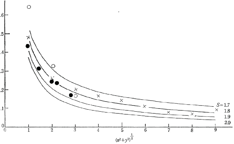
Figure 1: The first power-law fitting the spatial correlation function of the distribution of galaxies after deprojecting from an angular catalogue, reproduced from  VMtotsuji69 . The filled circles were obtained by Totsuji and Kihara, while the open circles and crosses were derived by Neyman, Scott and Shane under the assumption of their clustering model. The solid lines correspond to power-law correlation functions $xi(r)=(r_{0}/r)^{s}$ with the value of the exponent $s$ indicated in the legend.

This remarkable power-law for the two-point correlation function has dominated many of the analyses of the large scale structure for the past three decades and more.

Complementary to the Lick catalog, other surveys mapped the large scale distribution of clusters of galaxies, for example, the Palomar Observatory Sky Survey was used by George Abell to publish a catalogue of 2,712 clusters of galaxies VMabell58 . Some of them turned out not to be real clusters, but the majority were genuine. Analyses of this and other samples of galaxy clusters have yielded also power-law fits to the cluster-cluster correlation function $\xi_{cc}(r)$ but with exponents and amplitudes varying in a wider range, depending on selection effects, richness class, etc. VMpostman92 ; VMnichol92 ; VMdalton94 ; VMpostman99 ; VMborgani01 .

2 Redshift Surveys

Listing extragalactic objects and magnitudes as they appear projected onto the celestial sphere was just the first step towards obtaining a cartography of the universe. The second step was to obtain distances by measuring redshifts using spectroscopy for a large number of galaxies mapping large areas of the sky. This task provided information about how the universe is structured now and in the recent past. In the eighties, the Center for Astrophysics surveys played a leading role in the discovery of very large cosmic structures in the distribution of the galaxies. The first “slice of the universe” compiled by de Lapparent et al. VMlapparent86 extended up to 150 $h^{-1}$ Mpc, a deep distance at that time. The calculation of the correlation function – now in redshift space – of the CfA catalogue confirmed the power-law behaviour discovered by Totsuji and Kihara fourteen years before VMDP83 . It is worth to mention however that redshift distortions affect severely the correlation function at small separations and a distinction between redshift and real space became necessary.

The present wide field surveys are much deeper as it can be appreciated in Fig. 2 and in Fig. 3. Fig. 2 illustrates our local neighbourhood (up to $400\,h^{-1}\,\mathrm{Mpc}$) from the Two-Degree Field Galaxy Redshift Survey (2dFGRS) in a three dimensional view, where large superclusters surround more empty regions, delineated by long filaments. Fig. 3 shows the first CfA slice with cone diagrams from the 2dFGRS and the Sloan Didital Sky Survey (SDSS). The first one contains redshifts of about 250,000 galaxies in wide regions around the north and south Galactic poles with a median redshift $z=0.11$. It extends up to $z\simeq 3$. Galaxies in this survey go down to apparent blue magnitude $b_{\lim}=19.45$, therefore this is a magnitude-limited survey that misses faint galaxies at large distances, as it can be seen in Fig.  3. The SDSS survey is also magnitude-limited, but the limit has been selected to be red, $r_{\lim}=17.77$. The present release of the SDSS (DR6) covers an area almost five times as big as the area covered by the 2dFGRS.

More information about these surveys can be found in their web pages: http://www.mso.anu.edu.au/2dFGRS/ for the 2dF survey and http://www.sdss.org/ for the SDSS survey.

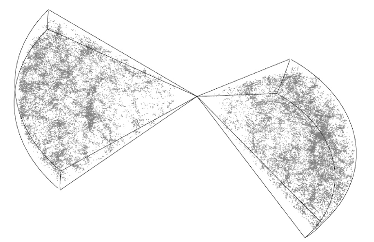
Figure 2: The two slices that conform the 2dfGRS showing the galaxy distribution up to a distance of $400\,h^{-1}\,\mathrm{Mpc}$. The left slice lies in the direction close to the North Galactic Pole, while the right one points towards the South Galactic Pole.

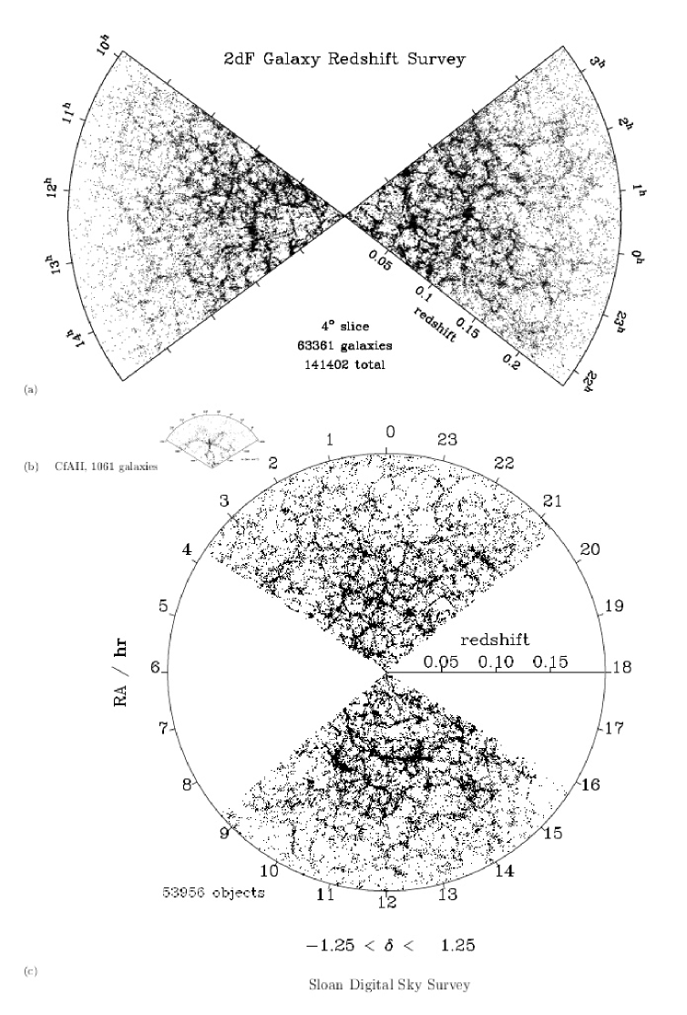
Figure 3: The top diagram shows two slices of $4^{\circ}$ width and depth $z=0.25$ from the 2dF galaxy redshift survey, from VMpeacock01 . The circular diagram at the bottom has a radius corresponding to redshift $z=0.2$ and shows 55,958 galaxies from the SDSS survey, from VMloveday ). As an inset, the first CfA slice from VMlapparent86 is shown to scale.

3 The Two-point Correlation Function

After measuring the two-point correlation function over projected galaxy samples, the great challenge was to do it directly for redshift surveys where the distance inferred from the recession velocities was used, providing a three-dimensional space. As it has been already mentioned, we have to bear in mind that measured redshifts are contaminated by the peculiar velocities. This 3D space, the so-called redshift space, is a distorted view of the real space. Fig.  4 shows a simulation with the effect of the peculiar velocities distorting the real space (left panel), squeezing the structures to produce the radial stretched structures pointing to the observer, known as fingers of God (right panel). For the details see the web page http://kusmos.phsx.ku.edu/~melott/redshift-distortions.html. These fingers of God appear strongest where the galaxy density is largest, and are attributable to the extra “peculiar” (ie:, non-Hubble) component of the velocity of individual galaxies in the galaxy clusters VMjackson72 ; VMsargent77 ; VMkaiser87 ; VMhamilton98 .

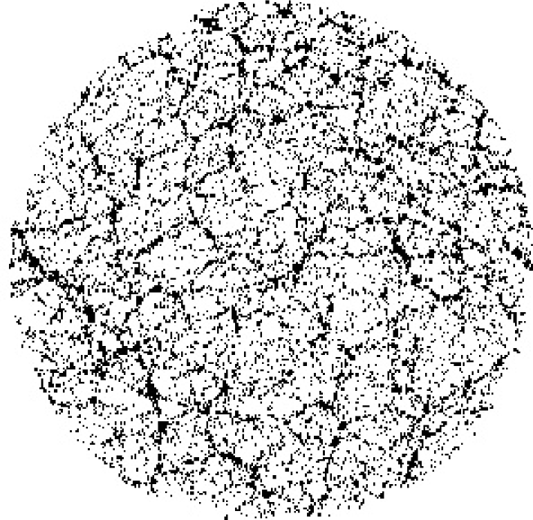
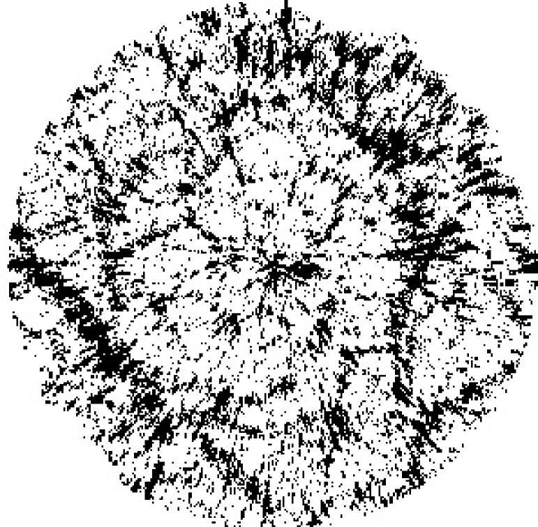
Figure 4: Illustration by a two-dimensional simulation of the effect of the peculiar velocities distorting the real space (left panel) to produce the redshift space (right panel). Figures courtesy of Adrian Melott.

Considering two infinitesimal volume elements $dV_{1}$ and $dV_{2}$ separated by a vector distance $\mathbf{r}_{12}$, the joint probability of there being a galaxy lying in each of these volumes is:

$$dP_{12}=n^{2}[1+\xi(\mathbf{r}_{12})]dV_{1}dV_{2},$$ (2)

Assuming homogeneity (the point process is invariant under translation) and isotropy (the point process is invariant under rotation) for the galaxy distribution, the quantity depends only on the distance $r_{12}=|\mathbf{r}_{12}|$ and Eq. (2) becomes Eq. (1).

Apart of the formal definitions given in the previous equations, to estimate the correlation function for a particular complete galaxy sample with $N$ objects, several formulae providing appropriate estimators have been introduced. The most widely used are the Hamilton estimator VMhamilton93 , and the Landy and Szalay estimator VMlandy93 . For both, a Poisson catalog, a binomial process with $N_{\rm{rd}}$ points, has to be generated within the same boundaries of the real data set. The estimators can be written as:

$$\widehat{\xi}_{\rm{HAM}}(r)={\frac{DD(r)\cdot RR(r)}{[DR(r)]^{2}}}-1,$$ (3)

$$\widehat{\xi}_{\rm{LS}}(r)=1+\left(\frac{N_{\rm{rd}}}{N}\right)^{2}\frac{DD(r)}{RR(r)}-2\frac{N_{\rm{rd}}}{N}\frac{DR(r)}{RR(r)}.$$ (4)

where $DD(r)$ is the number of pairs of galaxies of the data sample with separation within the interval $[r-dr/2,r+dr/2]$, $DR(r)$ is the number of pairs between a galaxy and a point of the Poisson catalog, and $RR(r)$ is the number of pairs between points from the Poisson catalog VMpons99 ; VMkerscher00 .

As it has been explained in the contributions by Hamilton and Szapudi in this volume, the above formulae have to be corrected due to the selection effects. These effects could be radial due to the fact that redshift surveys are built as apparent magnitude catalogs, and therefore fainter galaxies are lost at larger distances, and could be angular due to the Galactic absorption that makes the sky not equally transparent in all directions or to the fact that different areas of the sky within the sample boundaries are not equally covered by the observations, therefore providing varying apparent magnitude limit depending on the direction. Moreover some areas could not be covered at all because of the presence of nearby stars, or because of fiber collisions in the spectrograph. In order to account for this complexity the best solution is to use the freely available MANGLE software (http://space.mit.edu/home/tegmark/mangle/), a generic tool for managing angular masks on a sphere VMmangle .

3.1 The projected correlation function

Since at small scales, peculiar velocities strongly distort the correlation function, it has become customary to calculate and display the so-called projected correlation function

$$w_{p}(r_{p})=2\int_{0}^{\infty}\xi(\pi,r_{p})\mathrm{d}\pi,$$ (5)

where the two-dimensional correlation function $\xi(\pi,r_{p})$ is computed on a grid of pair separations parallel ($\pi$) and perpendicular ($r_{p}$) to the line of sight. Fig. 5 shows this function calculated by Peacock et al. VMpeacock01 for the 2dFGRS.

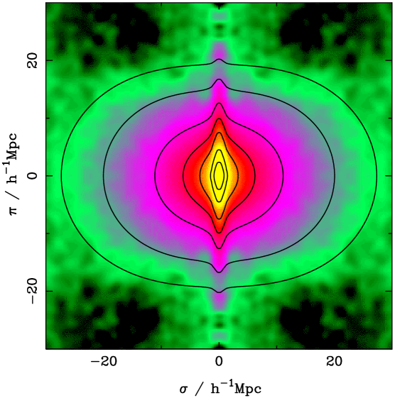
Figure 5: The galaxy correlation function $\xi(\pi,r_{p})$ for the 2dFGRS (transverse distance $r_{p}$ is represented here by $\sigma$). This diagram show the two sources of anisotropy in the correlation function: the radial smearing due to random velocities within groups and clusters at small distances and the large scale flattening produced by coherent infall velocities. In this diagram the calculation has been performed by counting pairs in boxes and then smoothing with a Gaussian. The results obtained for the first quadrant are repeated with reflection in both axes to show deviations from circular symmetry. Overplotted lines correspond to the function calculated for a given theoretical model. Figure from VMpeacock01 .

If the separation vector between two positions in redshift space is $\vec{s}=\vec{s_{2}}-\vec{s_{1}}$, and the line-of-sight vector is $\vec{l}=\vec{s_{1}}+\vec{s_{2}}$, the parallel and perpendicular distances of the pair are (see Fig. 6):

$$\pi=\frac{|\vec{s}\cdot\vec{l}|}{|\vec{l}|},\quad r_{p}=\sqrt{\vec{s}\cdot\vec{s}-\pi^{2}}.$$

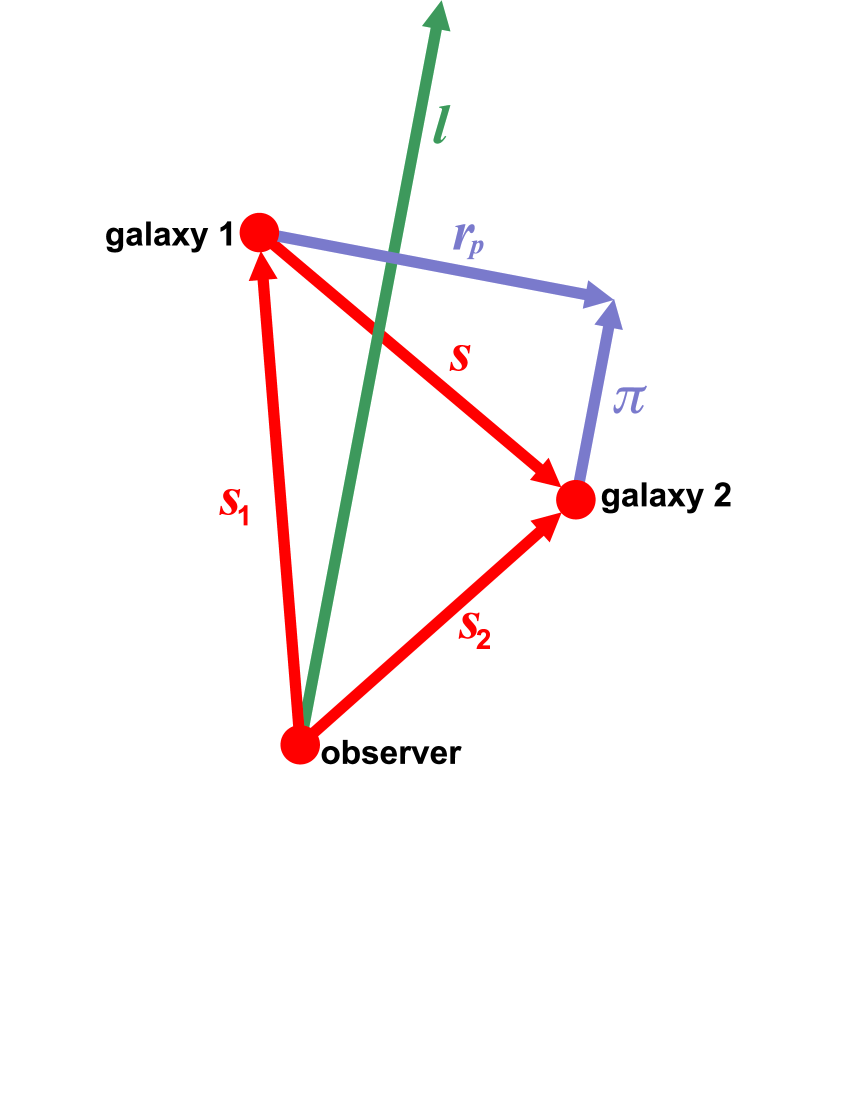
Figure 6: Illustration of the parallel and perpendicular separations between two objects.

Fig. 7 shows the projected correlation function calculated for the Sloan Digital Sky Survey by Zehavi et al. VMzehavi04 . The relation between the projected correlation function and the three-dimensional real correlation function (not affected by redshift distortions) is, for an isotropic distribution VMDP83 :

$$w_{p}(r_{p})=2\int_{r_{p}}^{\infty}\xi(r)\frac{r\mathrm{d}r}{\left(r^{2}-r_{p}^{2}\right)^{1/2}}.$$ (6)

From the previous equation it is straightforward to see that if $\xi(r)$ fits well a power law, i.e. $\xi(r)=(r/r_{0})^{-\gamma}$, $w_{p}(r_{p})$ also does, $w_{p}(r_{p})=Ar_{p}^{-\alpha}$, with

$$\alpha=\gamma-1,\quad\mbox{and}\quad A=\frac{r_{0}^{\gamma}\Gamma(0.5)\Gamma[0.5(\gamma-1)]}{\Gamma(0.5\gamma)}.$$

In practice, the integration in Eq. 5 is performed up to a fixed value $\pi_{\max}$ which depends on the survey. For the SDSS, Zehavi et al. VMzehavi04 used $\pi_{\max}=40\,h^{-1}\,\mathrm{Mpc}$, a value considered large enough by the authors to include the relevant information to measure $w_{p}(r_{p})$ in the range $0.1\,h^{-1}\,\mathrm{Mpc}<r_{p}<20\,h^{-1}\,\mathrm{Mpc}$. The assumed cosmological model for the calculation of distances is the concordance model for which $\Omega_{m}=0.3$ and $\Omega_{\Lambda}=0.7$.

The function shown in the left panel of Fig. 7 has been calculated making use of a subset containing 118,149 galaxies drawn from the flux-limited sample selected by Blanton et al. VMblanton03 . The estimator of the correlation function makes use of the radial selection function that incorporates the luminosity evolution model of Blanton et al. VMblanton03 . On the right panel the calculation has been performed over a volume-limited sample containing only galaxies bright enough to be seen within the whole volume (up to $462\,h^{-1}\,\mathrm{Mpc}$, the limit of the sample). This subsample contains 21,659 galaxies with absolute red magnitude $M_{r}<-21$ (for $h=1$). The solid line on the left panel of Fig. 7 shows the fit to $w_{p}(r_{p})$ which corresponds to a real-space correlation function $\xi(r)=(r/5.77\,h^{-1}\,\mathrm{Mpc})^{-1.80}$. For the volume-limited sample the fit shows a slightly steeper power-law $\xi(r)=(r/5.91\,h^{-1}\,\mathrm{Mpc})^{-1.93}$. This is a expected consequence of the segregation of luminosity as we will show later, since galaxies in this subsample are 0.56 magnitudes brighter than the characteristic value of the Schechter VMschechter76 luminosity function VMblanton03 .

Although it is remarkable from the power-law fits shown in Fig. 7 how the scaling holds for about three orders of magnitude in scale, the main point stressed in this analysis was precisely the unambiguous detection of a systematic departure from the simple power-law behaviour. A similar result was also obtained by Hawkins et al. VMhawkins03 for the 2dfGRS, although the best fit power-law for the correlation function of 2dF galaxies is $\xi(r)=(r/5.05\,h^{-1}\,\mathrm{Mpc})^{-1.67}$ with a less steep slope than the one found for SDSS galaxies and with a value of the correlation length $r_{0}=5.05\pm 0.26\,h^{-1}\,\mathrm{Mpc}$, substantially smaller than the SDSS result. Again, this can be explained as a consequence of the different galaxy content of both surveys, SDSS are red-magnitude selected while 2dF are blue-magnitude selected.

Error bars for the correlation function in Fig. 7 have been calculated in two different ways which illustrate the two main methods currently used. For the flux-limited sample, jackknife resampling of the data has been used. The sample is divided into $N$ disjoint subsamples covering each approximately the same area of the sky, then the calculation of $\xi(r)$ is performed on each of the jackknife samples created by summing up the $N$ subsamples except one, which is omitted in turn. The $ij$ element of the covariance matrix is computed by VMzehavi02

$$C_{ij}=\frac{N-1}{N}\sum_{k=1}^{N}({\xi_{i}}^{k}-{\bar{\xi}_{i}})({\xi_{j}}^{k}-{\bar{\xi}_{j}}),$$ (7)

where $\bar{\xi}_{i}$ is the average value of $\xi_{i}$ measured on the jackknife samples. Statistical errors can be calculated using the whole covariance matrix, or just making use of the elements in the diagonal, and thus ignoring the correlation amongst the errors. The other possibility consists in using mock catalogues from N-body simulations or semi-analytical models of structure formation with a recipe for allocating galaxies. These mock catalogues can be used as the subsamples in which Eq. 7 can be applied to obtain the covariance matrix.

The variation of the slope in the two-point correlation function of galaxies with the scale might be ascribed to the existence of two different clustering regimes: the small scale regime dominated by pairs of galaxies within the same dark matter halo and a second regime where pairs of galaxies belonging to different halos contribute to the downturn of the power-law in $w_{p}(r_{p})$.

Figure 7: The projected correlation function $w_{p}(r_{p})$ for the SDSS data. Left panel shows the result for the flux limited sample and right panel for the volume-limited sample. Two different power-law fits to the data have been performed. Solid lines make use of the full covariance matrix while dashed lines only use the diagonal elements. Figure from Zehavi et al. VMzehavi04 .

3.2 Galaxy properties and clustering

The photometric and spectral information provided by surveys like SDSS and 2dFGRS allows to study how the clustering of galaxies depends on different factors such as luminosity, morphology, colour and spectral type, although these factors are certainly not independent. For example, it is well known VMdavis76 ; VMdressler80 that early-type galaxies show more pronounced clustering at small separations than late-type galaxies, the first kind displaying steeper power-law fits to their correlation than the latter. This segregation plays an interesting role in the understanding of the galaxy formation process, since galaxies are biased tracers of the total matter distribution in the universe (mainly dark) and the bias also depends on the scale VMlahav02 . Madgwick et al. VMMadgwick03 have recently divided the 2dFGRS in two subsets: passive galaxies with a relatively low star formation rate, and active galaxies with higher current star formation rate. This division correlates well with colour and morphology, being passive galaxies mainly red old ellipticals.

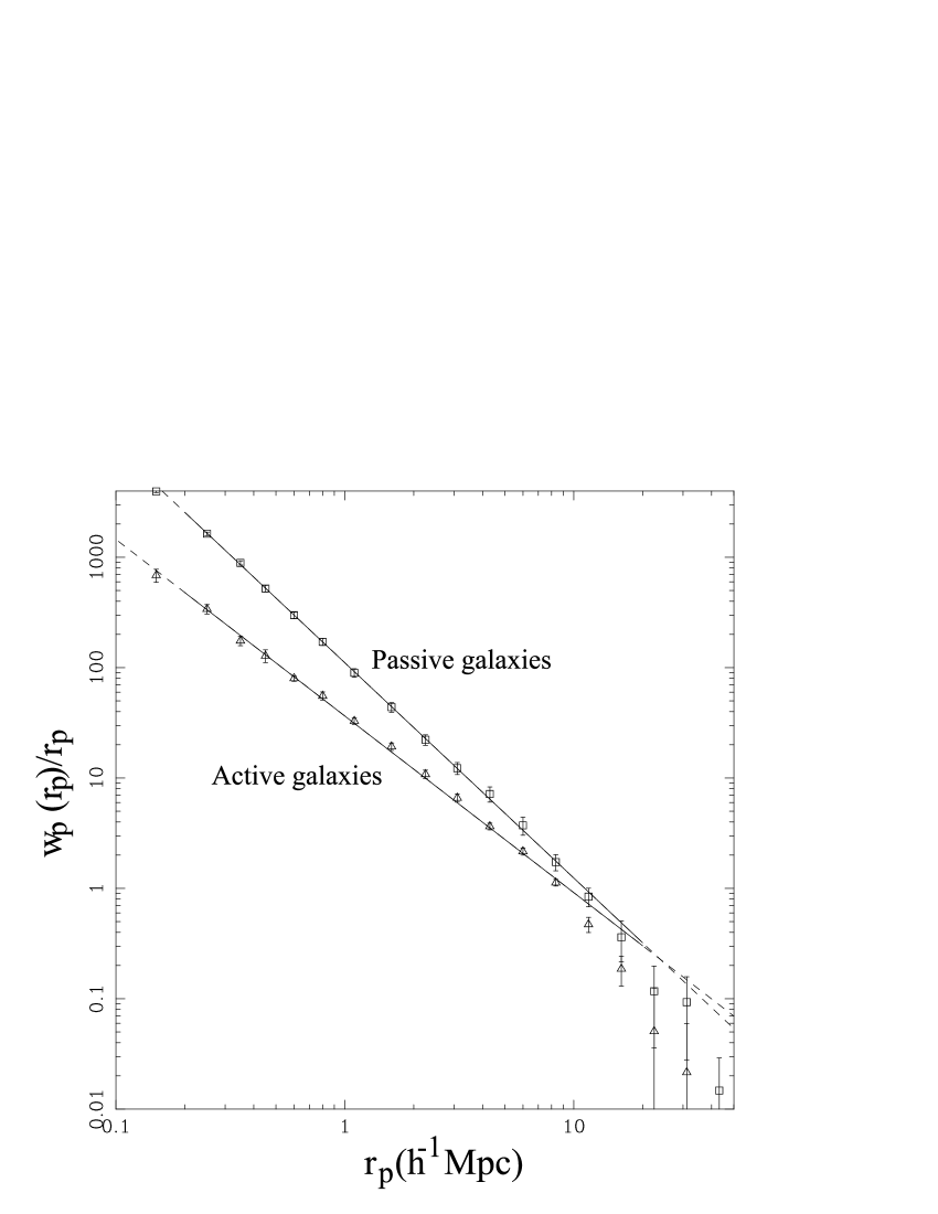
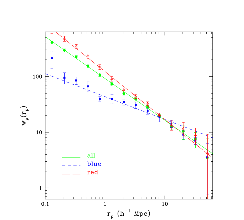
Figure 8: In the left panel, we show the projected correlation function $w_{p}(r_{p})$ for two subsamples of the 2dfGRS data where the division has been performed in terms of current star formation rate. Passive galaxies cluster stronger than their active counterparts. Figure adapted from Madgwick et al. VMMadgwick03 . In the right panel, it is shown the projected correlation function of subsamples divided by colour drawn from the SDSS. Different lines show the best-fit power-laws for $w_{p}(r_{p})$. The short-dashed, long-dashed and solid lines correspond to the blue, red, and full samples, respectively. Figure from Zehavi et al. VMzehavi02 .

Fig. 8 (left panel) shows the projected correlation function for these two subsets. As it can be appreciated, passive galaxies present a two-point correlation function with steeper slope and larger amplitude than active galaxies, being the best fit for each subsample $\xi(r)=(r/6.10\pm 0.34\,h^{-1}\,\mathrm{Mpc})^{-1.95\pm 0.03}$ for passive galaxies and $\xi(r)=(r/3.67\pm 0.30\,h^{-1}\,\mathrm{Mpc})^{-1.60\pm 0.04}$ for active galaxies. A similar analysis was also performed by Zehavi et al. VMzehavi02 dividing an early release of the SDSS galaxies into two subgroups by colour, red and blue, using the value of the colour $u^{*}-r^{*}=1.8$ for the division. The blue subset contains mainly late morphological types while the red group is formed mainly by bulge galaxies, as it should be expected. Again, as it can be appreciated in Fig. 8 (right panel), red galaxies cluster stronger than blue galaxies, being their best fit to a power-law in the range $[0.1\,h^{-1}\,\mathrm{Mpc}<r_{p}<16\,h^{-1}\,\mathrm{Mpc}]$, $\xi(r)=(r/6.78\pm 0.23\,h^{-1}\,\mathrm{Mpc})^{-1.86\pm 0.03}$, while for blue galaxies the best fit is $\xi(r)=(r/4.02\pm 0.25\,h^{-1}\,\mathrm{Mpc})^{-1.41\pm 0.04}$. Blanton et al. VMblanton05 have shown that large amplitudes in the correlation function corresponding to subsets selected by luminosity or colour are typically accompanied with steeper slopes.

4 The Power Spectrum

The power spectrum $P(k)$ is a clustering descriptor depending on the wavenumber $k$ that measures the amount of clustering at different scales. It is the Fourier transform of the correlation function, and therefore both functions contain equivalent information, although it can be said that they describe different sides of the same process. For a Gaussian random field, the Fourier modes are independent, and the field gets completely characterised by its power spectrum. As the initial fluctuations from the inflationary epoch in the universe are described as a Gaussian field, the model predictions in Cosmology are typically made in terms of power spectra.

The Power spectrum and the correlation function are related through a Fourier transform:

$$P({\mathbf{k}})=\int\xi({\mathbf{r}})e^{i{\mathbf{k}}\cdot{\mathbf{r}}}\,d^{3}r,$$

$$\xi({\mathbf{r}})=\int P({\mathbf{k}})e^{-i{\mathbf{k}}\cdot{\mathbf{r}}}\,\frac{d^{3}k}{(2\pi)^{3}},$$

Assuming isotropy, the last equation can be rewritten as:

$$\xi(r)=4\pi\int_{0}^{\infty}P(k)\frac{\sin(kr)}{kr}\frac{k^{2}\,dk}{(2\pi)^{3}}.$$

Some authors VMpeacock99 prefer to use the following normalization for the power spectrum:

$$\Delta^{2}(k)=\frac{1}{2\pi^{2}}P(k)k^{3},$$

in such a way that the total variance of the density field is just:

$$\sigma_{\delta}^{2}=\int_{0}^{\infty}\Delta^{2}(k)\,d(\ln k).$$

One of the advantages of the power spectrum over the correlation function is that amplitudes for different wavenumbers are statistically orthogonal (for a more detailed discussion see the contributions by Andrew Hamilton in this volume):

$$E\left\{\widetilde{\delta}({\mathbf{k}})\widetilde{\delta}^{\star}({\mathbf{k}}^{\prime})\right\}=(2\pi)^{3}\delta_{D}({\mathbf{k}}-{\mathbf{k}}^{\prime})P({\mathbf{k}}).$$ (8)

Here $\widetilde{\delta}({\mathbf{k}})$ is the Fourier amplitude of the overdensity field $\delta=(\rho-\bar{\rho})/\bar{\rho}$ at a wavenumber ${\mathbf{k}}$, $\rho$ is the matter density, a star denotes complex conjugation, $E\{\}$ denotes expectation values over realizations of the random field, and $\delta_{D}({\mathbf{x}})$ is the three-dimensional Dirac delta function.

If we have a sample (catalog) of galaxies with the coordinates ${\mathbf{x}}_{j}$, we can write the estimator for a Fourier amplitude of the overdensity distribution VMfkp (for a finite set of frequencies ${\mathbf{k}}_{i}$) as

$$F({\mathbf{k}}_{i})=\sum_{j}\frac{\psi({\mathbf{x}}_{j})}{\bar{n}({{\mathbf{x}}}_{j})}e^{i{\mathbf{k}}_{i}\cdot{\mathbf{x}}}-\widetilde{\psi}({\mathbf{k}}_{i}),$$

where $\bar{n}({\mathbf{x}})$ is the position-dependent selection function (the observed mean number density) of the sample and $\psi({\mathbf{x}})$ is a weight function that can be selected at will.

The raw estimator for the spectrum is

$$P_{R}({\mathbf{k}}_{i})=F({\mathbf{k}}_{i})F^{\star}({\mathbf{k}}_{i}),$$

and its expectation value

$$E\left\{\langle|F({\mathbf{k}}_{i})|^{2}\rangle\right\}=\int G({\mathbf{k}}_{i}-{\mathbf{k}}^{\prime})P({\mathbf{k}}^{\prime})\,\frac{d^{3}k^{\prime}}{(2\pi)^{3}}+\int_{V}\frac{\psi^{2}({\mathbf{x}})}{\bar{n}({\mathbf{x}})}\,d^{3}x,$$

where $G({\mathbf{k}})=|\tilde{\psi}({\mathbf{k}})|^{2}$ is the window function that also depends on the geometry of the sample volume. The reader can learn more about the estimation of the power spectrum in the contributions by Andrew Hamilton in this volume.

4.1 Acoustic peak in $\xi$ and acoustic oscillations in $P(k)$

Prior to the epoch of the recombination, the universe is filled by a plasma where photons and baryons are coupled. Due to the pressure of photons, sound speed is relativistic at this time and the sound horizon has a comoving radius of 150 Mpc. Cosmological fluctuations produce sound waves in this plasma.

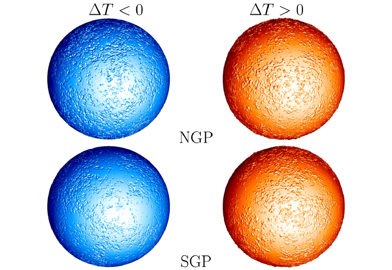
Figure 9: Temperature fluctuations of the WMAP data. The two upper spheres are centred in the north Galactic pole (NGP), while the bottom two are in the south Galactic pole (SGP). On the left hand side, in blue, pixels where $\Delta T<0$ are depicted as depths, while on the right hand side, red pixels with $\Delta T>0$ are displayed as elevations. The “sea level” in blue spheres corresponds to the pixels where $\Delta T\geq 0$ and in the red sphere, where $\Delta T\leq 0$.

At about 380,000 years after the Big Bang, when the temperature has fallen down to 3000 K, and recombination takes place, the universe loses its ionized state and neutral gas dominates. At this state, sound speed drops off abruptly and acoustic oscillations in the fluid become frozen. Their signature can be detected in both the Cosmic Microwave Background (CMB) radiation and the large-scale distribution of galaxies. Fig. 9 shows a representation of the temperature at the last scattering surface from WMAP. These fluctuations have been analyzed in detail to obtain a precise estimation of the anisotropy power spectrum of the CMB. The acoustic peaks in this observed angular power spectrum (see contribution by Enrique Martínez-Gónzalez in this volume) have become a powerful cosmological probe. In particular, the CMB provides an accurate way to measure the characteristic length scale of the acoustic oscillations, that depends on the speed of sound, $c_{s}$, in the photon-baryon fluid and the cosmic time when this takes place. The distance that a sound wave has traveled at the age of the universe at that time is

$$\int_{0}^{t_{rec}}c_{s}(t)(1+z)dt\simeq 147\pm 2\,\,\mbox{Mpc}.$$ (9)

for the standard flat $\Lambda$-CDM model. This fixed scale imprinted in the matter distribution at recombination can be used as a “standard ruler” for cosmological purposes.

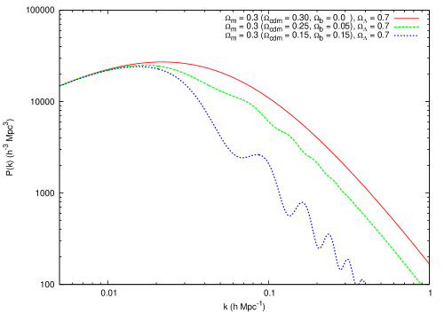
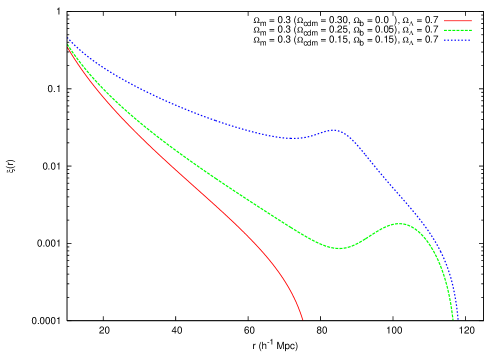
Figure 10: Top panel. The linear-regime power spectrum of the matter in the universe for different flat models with $\Omega_{\rm total}=1,\,h=0.7$,   $\Omega_{m}=0.3$ and $\Omega_{\Lambda}=0.7$. The three curves correspond to different proportions of baryonic and cold dark matter: from top to bottom $\Omega_{b}=0,0.05,0.15$. As we see, increasing the baryon content (at fixed $\Omega_{m}$) increases the amplitude of the acoustic oscillations, while suppresses power on small scales (large wavenumber). In the bottom panel, it is shown the corresponding correlation function to each model displayed with the same line style. For no baryons (pure cold dark matter), the acoustic peak is missing, while the peak amplitude is larger with a larger proportion of baryons. Data for the figure courtesy of Gert Hütsi. A similar diagram can be found in VMnichol07 and VMeis98 .

The imprint in the matter distribution of this acoustic feature should be detected in both the correlation function and the matter power spectrum. However, the amplitude of the acoustic peaks in the CMB angular power spectrum is much larger than the expected amplitude of the oscillations in the matter power spectrum, which are called for obvious reasons baryonic acoustic oscillations (BAOs) Moreover, the feature should be manifested as a single peak in the correlation function at about 100 $h^{-1}$ Mpc, while in the power spectrum it should be detected as a series of small-amplitude oscillations as it is shown in Fig. 10. Baryons represent only a small fraction of the matter in the universe, and therefore, as it can be appreciated in the figure, the amplitude of the oscillations in the power spectrum are rather tiny for the concordance model (green dashed line in the top panel of Fig. 10). We can see how increasing the baryon fraction increases the amplitude of the oscillations, while wiggles disappear for a pure $\Lambda$-CDM model (with no baryonic content). At small scales the oscillations are erased by Silk damping, therefore one needs to accurately measure the power-spectrum or the correlation function on scales between $50-150\,h^{-1}$ Mpc to detect theses features.

Eisenstein et al. (2005) VMeisenstein05 announced the detection of the acoustic peak in the two-point redshift-space correlation function of the SDSS LRG survey (see Fig. 11). More or less simultaneously, Cole et al. (2005) VMcole05 discovered the corresponding feature in form of wiggles of about 10% amplitude in the power spectrum of 2dF galaxy redshift survey. We have also calculated the redshift correlation function for a nearly volume-limited sample of the 2dFGRS extracted by Croton et al. VMcroton04 . There are about 25,000 galaxies in this sample with absolute magnitude within the range $-20>M_{B_{J}}-5\log_{10}h>-21$. The correlation function displayed in the right panel of Fig.11 shows a prominent peak around $100\,h^{-1}$ Mpc which expands for a wider scale range that the bump observed in the SDSS-LRG sample (left panel). This could be due to scale-dependent differences between the clustering of the two samples. A similar effect has been recently observed in the power spectrum VMsanchez08 of the two surveys (see also the figure caption of Fig. 12). Of course, the statistical significance of this feature is still to be tested. Interestingly enough is the fact that the mock catalogues generated by Norberg et al. VMnorberg02 to mimic the properties of the 2dFGRS at small scales do not show the acoustic peak. Moreover, we can see a large scatter in the correlation function of the mocks, with average values that do not follow the data (mocks show larger correlations at intermediate scales and smaller at large scales).

Fig. 12 shows the power spectrum calculated recently by Sánchez and Cole VMsanchez08 for the 2dFGRS and the SDSS-DR5 survey. The expected acoustic oscillations are clearly detected within the error bands. These errors have been calculated using mock catalogues generated from lognormal density fields with a given theoretical power spectrum.

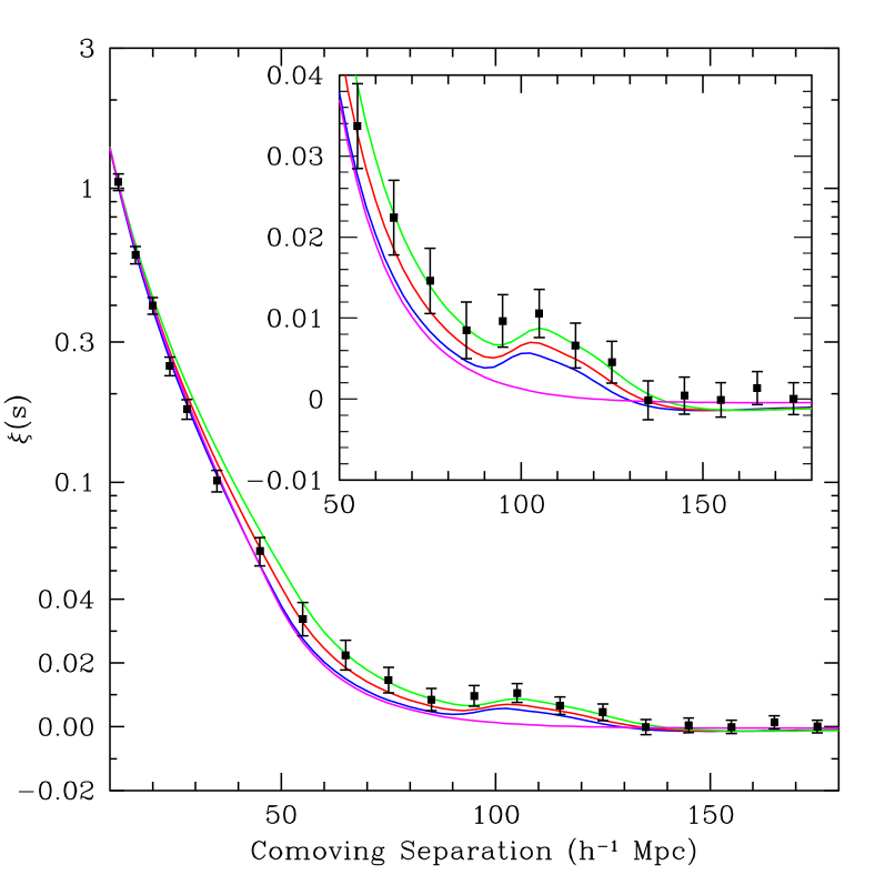
Figure 11: Left. The redshift-space galaxy correlation function measured for the LRG SDSS sample containing 46,748 luminous read galaxies in redshift space. The vertical axis mixes logarithmic and linear scales.The inset shows an expanded view around the peak ($\sim 100\,h^{-1}$ Mpc) with the vertical axis in linear scale. The different solid curves correspond to a $\Lambda$-CDM model with $\Omega_{m}h^{2}=0.12$ (green), 0.13 (red), 0.14 (blue); in all cases the baryon content is fixed to $\Omega_{b}h^{2}=0.024$). The magenta line corresponds to a pure $\Lambda$-CDM model with no baryons. Figure from Eisenstein et al. VMeisenstein05 . Right. The redshift-space galaxy correlation function measured for a volume-limited sample extracted from the 2dFGRS (solid discs joined by a solid line). The same function has been calculated on the 22 mocks models explained in the text. The average correlation function together with 1-$\sigma$ deviations are shown in the diagram. Mocks do not show the peak detected in the real galaxy survey.

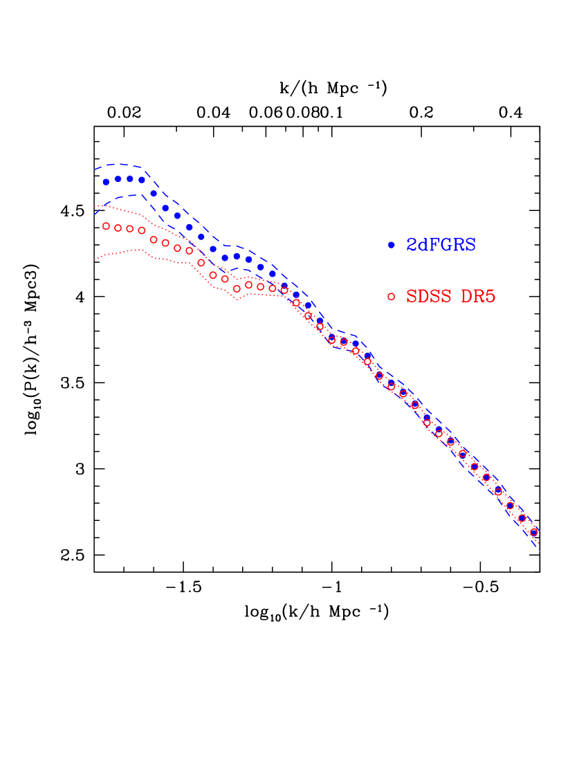
Figure 12: The matter power spectrum $P(k)$ for the 2dFGRS and the SDSS-DR5. The agreement is good at small scales, while at larger scales there is a clear evidence of SDSS having more small-scale power than 2dfGRS. Sánchez and Cole VMsanchez08 interpret this result as a consequence of the stronger scale-dependent bias shown by the red galaxies that dominate the SDSS catalogue. Figure adapted from Sánchez and Cole VMsanchez08 .

4.2 Concluding remarks and challenges

The expected value of the sound horizon at recombination (Eq. 9) determined from the CMB observations can be compared with the observed BAO scale in the radial direction at a given redshift to estimate the variation of the Hubble parameter with redshift $H(z)$. High accurate redshifts are needed to carry on this test. Likewise, the BAO scale observed in redshift surveys compared with its expected value provides us with a way to measure the angular diameter distance, as a function of redshift $D_{A}(z)$. As Nichols VMnichol07 points out this is similar, in a sense, to the measurement of the correlation function in the parallel and perpendicular directions to the line of sight, $\xi(\pi,r_{p})$, explained in Sec. 3.1.

There are several ongoing observational projects that will map a volume large enough to accurately measure BAOs in the galaxy distribution, some of them making use of spectroscopic redshifts (i.e., AAT WiggleZ, SDSS BOSS, HETDEX, and WFMOS) and others making use of photometric redshifts (i.e., DES, LSST, Pan-STARRS, and PAU), all of them surveying large areas of the sky and encompassing volumes of several Gpc³. For an updated review see VMfrieman08 . To deal with the uncertainties of the BAO measurement due to different effects (non-linear gravitational evolution, biasing of galaxies with respect to dark matter, redshift distortions, etc.) is not easy, and accurate cosmological simulations are required for this purpose.

The correlation function can be generalized to higher order (see the contribution by Istvan Szapudi in this volume): the $N$-point correlation functions. This allows to statistically characterize the galaxy distribution with a hierarchy of quantities which progressively provide us with more and more information about the clustering of the point process. These measures, however, had been difficult to derive with reliability from the scarcely populated galaxy catalogs. The new generation of surveys will surely overcome this problem.

There are, nevertheless, other clustering measures which provide complementary information to the second-order quantities described above. For example, the topology of the galaxy distribution measured by the genus statistic provides information about the connectivity of the large-scale structure. The topological genus of a surface is the number of holes minus the number of isolated regions plus 1. This quantity is calculated for the isodensity surfaces of the smoothed data corresponding to a given density threshold (excursion sets). The genus can be considered as one of the four Minkowski functionals used commonly in stochastic geometry to study the shape and connectivity of union of convex three-dimensional bodies. In 3-D there are four functionals: the volume, the surface area, the integral mean curvature, and the Euler-Poincaré characteristic, related with the genus of the boundary (see the contribution by Enn Saar in this volume).

The use of wavelets and related integral transforms is an extremely promising tool in the clustering analysis of 3-D catalogs. Some of these techniques are introduced in the contributions by Bernard Jones, Enn Saar and Belen Barreiro in this volume.

Acknowledgements
I thank Enn Saar, Carlos Peña and Pablo Arnalte for useful comments and suggestions on the manuscript, Gert Hütsi for the data for Fig. 10, Fernando Ballesteros and Silvestre Paredes for help with the figures, and Pablo de la Cruz, and María Jesús Pons-Bordería for allowing me to use unpublished common work on the analysis of the large-scale correlation function of the 2dFGRS in this review. I acknowledge financial support from the Spanish Ministerio de Educación y Ciencia project AYA2006-14056 (including FEDER) and the Acción Complementaria AYA2004-20067-E.

References

- (1) Abell, G. O. 1958, ApJS , 3, 211
- (2) Blanton, M. R., et al. 2003, ApJ , 592, 819
- (3) Blanton, M. R., et al. 2005, ApJ , 629, 143
- (4) Borgani, S., & Guzzo, L. 2001, Nature, 409, 39
- (5) Cole, S., et al. 2005, MNRAS , 362, 505
- (6) Croton, D. J., et al. 2004, MNRAS , 352, 828
- (7) Dalton, G. B., Croft, R. A. C., Efstathiou, G., Sutherland, W. J., Maddox, S. J., & Davis, M. 1994, MNRAS , 271, L47
- (8) Davis, M., & Geller, M. J. 1976, ApJ , 208, 13
- (9) Davis, M., & Peebles, P. J. E. 1983, ApJ , 267, 465
- (10) de Lapparent, V., Geller, M. J., & Huchra, J. P. 1986, ApJ , 302, L1
- (11) Dressler, A. 1980, ApJ , 236, 351
- (12) Eisenstein, D. J. et al., 2005, ApJ , 633, 560
- (13) Eisenstein, D. J., & Hu, W. 1998, ApJ , 496, 605
- (14) Feldman, H. A., Kaiser, N., & Peacock, J. A. 1994, ApJ , 426, 23
- (15) Frieman, J. A., Turner, M. S., & Huterer, D. 2008, ArXiv e-prints:0803.0982
- (16) Hamilton, A. J. S. 1993, ApJ , 417, 19
- (17) Hamilton, A. J. S. 1998, in The Evolving Universe, Astrophysics and Space Science Library vol. 231, ed. by D.Hamilton, Kluwer, Dordrecht, p. 185
- (18) Hawkins, E., et al. 2003, MNRAS , 346, 78
- (19) Hubble, E. 1934, ApJ , 79, 8
- (20) Jackson, J. C. 1972, MNRAS , 156, 1P
- (21) Jones, B. J. T., 2001, in Historical Development of Modern Cosmology, ed. by Martínez, V. J. et al., ASP conference series, vol. 252, p. 245
- (22) Jones, B. J. T., Martínez, V. J., Saar, E., & Trimble, V., 2004, Rev. Mod. Phys., 76, 1211
- (23) Kaiser, N. 1987, MNRAS , 227, 1
- (24) Kerscher, M., Szapudi, I., & Szalay, A. S. 2000, ApJ , 535, L13
- (25) Lahav, 0., et al. 2002, MNRAS , 333, 961
- (26) Landy, S. D., & Szalay, A. S. 1993, ApJ , 412, 64
- (27) Limber, D. N. 1954, ApJ , 119, 655
- (28) Loveday, J. 2002, Contemporary Physics, 43, 437
- (29) Madgwick, D. S., et al. 2003, MNRAS , 344, 847
- (30) Martínez, V. J. & Saar, E., 2002, Statistics of the Galaxy Distribution, Chapman & Hall /CRC Press, Boca Raton
- (31) Navarro, J. F., Frenk, C. S., & White, S. D. M., 1997, ApJ , 490, 493
- (32) Neyman, J., & Scott, E. L. 1952, ApJ , 116, 144
- (33) Neyman, J., Scott, E. L., & Shane, C. D. 1953, ApJ , 117, 92
- (34) Nichol, R. C., Collins, C. A., Guzzo, L., & Lumsden, S. L. 1992, MNRAS , 255, 21P
- (35) Nichol, R. C. 2007, ArXiv e-prints:0708.2824
- (36) Norberg, P., et al. 2002, MNRAS , 336, 907
- (37) Peacock, J. A., 1999, Cosmological Phyiscs, Cambridge University Press, Cambridge
- (38) Peacock, J. A., et al. 2001, Nature, 410, 169
- (39) Peebles, P. J. E., 1974, A&A , 32, 197
- (40) Peebles, P. J. E., 1980, The Large-Scale Structure of the Universe, Princeton University Press, Princeton
- (41) Pons-Bordería, M.-J., Martínez, V. J., Stoyan, D., Stoyan, H., & Saar, E. 1999, ApJ , 523, 480
- (42) Postman, M., Huchra, J. P., & Geller, M. J. 1992, ApJ , 384, 404
- (43) Postman, M. 1999, in Evolution of Large Scale Structure: From Recombination to Garching, ed. by A. J. Banday, R. K. Sheth, and L. N. da Costa, p. 270
- (44) Rubin, V. C., 1954, Proceedings of the National Academy of Science, 40, 541
- (45) Sánchez, A. G., & Cole, S. 2008, MNRAS , 385, 830
- (46) Sargent, W. L. W., & Turner, E. L. 1977, ApJ , 212, L3
- (47) Schechter, P. 1976, ApJ , 203, 297
- (48) Shane, C. D. & Wirtanen, C. A., 1967, Publ. Lick Obs. 22, 1
- (49) Seljak, U. 2000, MNRAS, 318, 203
- (50) Swanson, M. E. C., Tegmark, M., Hamilton, A. J. S., & Hill, J. C. 2007, ArXiv e-prints:0711.4352
- (51) Totsuji, H. & Kihara, T. 1969, Pub. Astron. Soc. Japan, 21, 221
- (52) Zehavi, I., et al. 2002, ApJ , 571, 172
- (53) Zehavi, I., et al. 2004, ApJ , 608, 16
- (54) Zwicky, F., 1953, Helv. Phys. Acta, 26, 241