Estimating a cosmic ray detector exposure sky map under the hypothesis of seasonal and diurnal effects factorization

Abstract

The measurement of large scale patterns or anisotropies in the arrival direction of high energy cosmic rays is an important step towards the understanding of their origin. Such measurements rely on an accurate estimation of the detector relative exposure in each direction on the sky: the coverage map. To reach an accuracy on the determination of this map below the 1% level one must properly identify and correct for all the environmental effects that may induce variations in the detector exposure as a function of time. In an approach, similar to the one used in anti-sidereal time analysis, we propose a method to empirically estimate and correct for those effects under the hypothesis that seasonal and diurnal variations can be factorized. We tested this method using a model ground detector of cosmic ray air showers, whose aperture varies due to the dependence of the air shower development on the atmospheric conditions.

^1,2, ^1,2 and ¹

1 Introduction

Large scale anisotropy studies play an important role in the search for the origin of the highest energy cosmic rays. While some results [1] have favored a scenario with a $\sim$4% dipole pointing towards the Galactic Center and the Cygnus region at EeV (1 EeV = $10^{18}$ eV) energies, analyses with Auger data [2] have shown consistency with isotropy in this region of the sky. A series of large scale complementary analyses with the first two years of Auger data was performed in [3], focusing on right ascension modulations and carefully accounting for systematic effects, showing as well no indication of significant anisotropy at EeV energies. At the PeV (1 PeV = $10^{15}$ eV) range, the Rayleigh formalism applied to right ascention modulations of the KASCADE experiment also shows no hints of anisotropies, both for light and heavy primaries [4].

In the $10^{11}-10^{14}$ eV range, underground muon and Extensive Air Shower (EAS) detectors were able to shed some light into the nature of large scale anisotropies at these energies [5, 6, 7, 8]. For energies $\sim 10^{11}$ eV, explored mainly by shallow underground muon detectors, cosmic rays are believed to be modulated by solar magnetic fields, whereas for energies $\sim 10^{14}$ eV, dominated by EAS arrays, the primaries will feel essentially the local structure of the galactic magnetic field. Amplitudes of right ascention modulations measured in these two energy ranges are $\sim 10^{-4}$ and $\sim 10^{-3}$, respectively. An Earth based detector moving through an isotropic cosmic ray plasma at rest will register an intensity modulation due to the Earth’s rotation around its axis, the Compton-Getting (CG) effect [9]. For the movement of the Earth around the Sun, the CG effect should give rise to a solar diurnal modulation. In fact, solar diurnal variations measured at $\sim 10$ TeV [7] (1 TeV = $10^{12}$ eV) are consistent with such an expectation. In a similar way, in the cosmic ray plasma rest frame, the movement of the whole solar system around the galactic center could give rise to a similar CG effect, however, now the modulations should be seen in sidereal time. Analysis in the $\sim 300$ TeV range [10] showed no such modulations, indicating that at theses energies, cosmic rays corotate with the solar system trapped by the local galactic field inside the arm.

In the energy interval $10^{14}$ - $10^{15}$ eV, linking the two ranges discussed in the first and second paragraphs of this section, the EAS-TOP collaboration has reported a solar time modulation of amplitude $\sim 3\times 10^{-4}$, in very good agreement with the expected value from the CG effect [11]. Up to $10^{14}$ eV, a clear signal of sidereal modulation at the $\sim 3\times 10^{-4}$ level were also seen by this experiment, and above 300 TeV the amplitudes are not significant, showing consistency with the Tibet results.

Although one-dimensional methods, such as the first harmonic analysis (in the case of a uniform right ascention exposure detector) of the Rayleigh formalism, the differential East-West method [8] and the Fourier transform method of modified times [12], are quite powerful in identifying distortions in the right ascention or sidereal time distributions, a complete caracterization of large scale anisotropies rely on the accurate knowledge of the detector relative exposure in all visible directions of the sky, the two-dimensional coverage map. The proper estimation of this map is a very challenging experimental task. All changes in the local (Earth based) running conditions of the detector that may impact on the exposure must be identified and taken into account. A perfect coverage map should contain all variations induced by local effects and none of those coming from the sky. In such an ideal case, the excess maps, i.e. the ratio of the observed signal over the estimated coverage in each direction of the sky, will only show the true sky anisotropies.

The exposure in a given direction of the sky will be a function with a geometrical part depending on the local detection angles: the zenith angle $\theta$ and the azimuth $\phi$, and a part depending on time. Even though our knowledge on extensive air shower development through the atmosphere has clearly increased in the last decades, it is still incomplete and Monte Carlo approaches, in addition to being computationally demanding, have a range of applicability limited to the cases where the accuracy required is not so much lower than just a few percent. Therefore, in the calculation of the geometrical and time acceptances, methods which can use directly the data are very appreciated [13, 14]. Obviously, such data based methods will face us with subtle effects, since the sample from which we are trying to extract the exposure, contains, in principle, the sky anisotropy which we wish to later estimate. The usual procedure applied to build the exposure map from the data itself is to perform some kind of scrambling into the local angles and arrival times in order to wash out the possible sky anisotropies and retain only the local features [15]. The role played by the time behaviour of the detector is therefore central in calculating the sky exposure map since, on the one hand, detector long term variability induces fake anisotropic patterns on the sky, while on the other hand, large scale anisotropy can distort the time distribution of events registered by a stably running detector. As an example of the former effect, we know that a solar modulation superimposed on the top of a seasonal envelope, both genuine local weather effects, will give rise to an apparent sidereal modulation. And for the latter, it is widely known that any modulation in right ascension will appear as a sidereal variation in the time distribution of events.

In this article we will deal only with the time variation of the exposure as this is usually the most delicate issue. Our method can be applied to any kind of detector with nearly time independent aperture, a typical property of ground arrays where the detector has, in principle, 100% duty cycle. Through the text, just for illustration purposes, we are going to work with a cosmic ray detector located at the same position of the Auger Observatory [16], but the results should be valid for a large variety of detectors.

The paper is organised as follows: we present the basic underlying assumption of Julian day $\times$ solar factorization of the detector rate in section 2, and in section 3 we show how to recover the time detector distribution from the dataset itself if the possible sky anisotropies, through their sidereal amplitudes, are no larger than just a few percent, therefore avoiding the use of Monte Carlo simulation. The residual systematic effects in the coverage due to possible non-factorizable components of the detector rate is estimated in section 4 by using a model for the detector rate based on weather monitoring data taken at the Auger site. The robustness of coverage maps built under the factorization hypothesis is treated in section 5 by reconstructing some anisotropic patterns on the sky. We finally conclude in section 6.

2 The Factorizable Acceptance Model (FAM)

Let ${\cal A}$ be the detection efficiency of a surface array. This function depends on the time $t$, on the shower horizontal coordinates $\theta$ and $\phi$ and on a set of parameters, like the energy, which we will refer to as X. By writing the time as a function of two distinct variables: $t=t(j,s)$, where $j$ is the Julian day and $s$ is the solar time, we can therefore represent the array efficiency as ${\cal A}(j,s,\theta,\phi,\mathbf{X})$.

In the most general case, the efficiency will have an intricate form with non-trivial correlations among all the parameters. For example, at a fixed energy, the weather induced time modulations might have a relative amplitude which depends on the zenith angle. In the following, one assumes that the domain spanned by the variables $\{\theta,\phi,\mathbf{X}\}$ can be broken up into complementary regions over which ${\cal A}$ can be factorized as

$${\cal A}(j,s,\theta,\phi,\mathbf{X})={\cal A}_{t}(j,s)\times{\cal A}_{\Omega}(\theta,\phi,\mathbf{X}),$$ (1)

where ${\cal A}_{t}(j,s)$ and ${\cal A}_{\Omega}(\theta,\phi,\mathbf{X})$ are both dimensionless, and the results are given for only one of such regions. In practice, to get the full picture, one does the same analysis over all regions required to be defined.

In the factorizable acceptance model (FAM), we assume that the time variation of the efficiency is the product of a daily variation in solar time $\eta_{D}(s)$ and a seasonal variation in Julian days $\eta_{Y}(j)$, so that one can write

$${\cal A}_{t}(j,s)=\eta_{Y}(j)\times\eta_{D}(s).$$ (2)

The hypothesis behind this factorization is that what happens during a day is not exclusive to that particular day, but mainly correlated to the sun altitude in the sky (given by the solar time) in that day. The validity of such a hypothesis can be checked directly from the data set as will be shown in section 4.

3 Extracting the acceptance under the FAM hypothesis from the data set itself

The goal of this section is to show how one can retrieve the time modulations of the detector acceptance from the data set itself, if one uses an integer number of data taking years and if a possible anisotropic pattern on the sky has a small amplitude, that is, a sidereal time modulation no larger than a few percent. For ultra high energy cosmic rays, this is in fact a pretty good assumption.

Let ${\cal F}(\alpha,\delta,\mathbf{X})$ be the cosmic ray flux from the direction $(\alpha,\delta)$ in equatorial coordinates, where $\alpha$ is the right ascension and $\delta$ is the declination, reaching the Earth per unit time, area, solid angle and per units of $\mathbf{X}$. The variables $\alpha$ and $\delta$ can be written in terms of the local horizontal coordinates $\theta$, $\phi$ and the time of detection $t(j,s)$. Therefore, the following integral over one of the regions where the factorization (1) is valid

$$\Phi(t)=\int\limits_{\mathbf{X}}\int\limits_{\Omega}{\cal A}_{\Omega}(\theta,\phi,\mathbf{X}){\cal F}(\alpha(t,\theta,\phi),\delta(t,\theta,\phi),\mathbf{X})d\mathbf{X}d\Omega,$$ (3)

has dimension of number of particles per unit time and area. The rate of cosmic rays detected (over the region where $\Phi(t)$ is defined) as a function of time is then given by

$${\cal R}(t)={\cal R}(j,s)={\cal A}_{t}(j,s)\times\Phi(t)\times S_{eff}(t),$$ (4)

where $S_{eff}(t)$ represents here the instantaneous effective area of the detector, since this might not be constant in time, as is the case of detectors which take data as their sizes are still growing by the installation of new detection units, or experimental problems which might black part of the detector, reducing its effective area. These effects can usually be corrected for and we will not be concerned with them in this paper.

The function $\Phi(t)$ gives us the time dependence of the sky anisotropy and can be written in terms of the sidereal time $t_{sid}$ as

$$\Phi(t_{sid})=\Phi_{0}\left[1+\epsilon(t_{sid})\right],$$ (5)

where $\epsilon(t_{sid})$ is a function of period $D_{sid}$ (a sidereal day) with null integral over this time interval and $|\epsilon|<<1$ and

$$\Phi_{0}=\frac{1}{D_{sid}}\int\limits_{D_{sid}}\Phi(t_{sid})dt_{sid},$$ (6)

Since a Julian day is about only 4 minutes longer than a sidereal day (a correction factor of about 1 + 1/365.25) and a calendar year being a little longer than the time it takes for $t_{sid}$ to span the whole sky in right ascension (same correction), we have two useful approximations

$$\int\limits_{Y_{sol}}\epsilon(t_{sid})dt_{sid}\simeq 0,\quad\textrm{and}\quad\int\limits_{D_{sol}}\epsilon(t_{sid})dt_{sid}\simeq 0,$$ (7)

where $Y_{sol}$ and $D_{sol}$ are the durations of a solar year and a solar day, respectively.

By explicitly writing the average values of $\eta_{Y}(j)$ and $\eta_{D}(s)$, we have

$$\eta_{Y}(j)=\overline{\eta}_{Y}\left(1+f_{Y}(j)\right)\quad\textrm{and}\quad\eta_{D}(s)=\overline{\eta}_{D}\left(1+f_{D}(s)\right),$$ (8)

and by definition the fractional amplitudes satisfy

$$\int\limits_{Y_{sol}}f_{Y}(j)dj=0,\quad\textrm{and}\quad\int\limits_{D_{sol}}f_{D}(s)ds=0,$$ (9)

With all that in mind, we can write the rate of cosmic rays, corrected by the effective array surface as

$${\cal R}^{{}^{\prime}}(j,s) = \frac{{\cal R}(j,s)}{S_{eff}(j,s)}$$ (10)

$$= \overline{\eta}_{Y}\overline{\eta}_{D}\Phi_{0}\left[1+\epsilon(t_{sid})\right]\left[1+f_{Y}+f_{D}+f_{Y}f_{D}\right],$$

where we have omitted the dependence of $f_{Y}$ and $f_{D}$ on $j$ and $s$, respectively. Integrating over a solar day or a solar year and using eqs. (7) and (9), we obtain the functions ${\cal R}_{Y}^{{}^{\prime}}(j)=\int\limits_{D_{sol}}{\cal R^{\prime}}(j,s)ds$ and ${\cal R}_{D}^{{}^{\prime}}(s)=\int\limits_{Y_{sol}}{\cal R^{\prime}}(j,s)dj$

$${\cal R}_{Y}^{{}^{\prime}}(j)=\Phi_{0}\overline{\eta}_{D}D_{sol}\left[1+\frac{1}{D_{sol}}\int\limits_{D_{sol}}\epsilon(t_{sid})f_{D}(s)ds\right]\eta_{Y}(j)$$ (11)

$${\cal R}_{D}^{{}^{\prime}}(s)=\Phi_{0}\overline{\eta}_{Y}Y_{sol}\left[1+\frac{1}{Y_{sol}}\int\limits_{Y_{sol}}\epsilon(t_{sid})f_{Y}(j)dj\right]\eta_{D}(s).$$ (12)

We are specifically interested in the estimation of the coverage map for cosmic rays at energies above around $10^{17}$ eV, detected by cosmic rays detectors such as large surface arrays. As already mentioned, such arrays are quite stable in time, with typical fractional amplitudes for the time variations in the detection efficiency which are no larger than 10% (a total 20% variation) along a day or a year (see section 4). Moreover, the sidereal time modulation at these energies will not exceed the 5% level, a somewhat exaggerated scenario (see footnote on page 1). Under these hypotheses the integral inside square brackets can be neglected, since it will be certainly below the 0.5% level.

Therefore, one can write

$${\cal R}_{Y}^{{}^{\prime}}(j)\simeq\Phi_{0}\overline{\eta}_{D}D_{sol}\eta_{Y}(j),\quad{\cal R}_{D}^{{}^{\prime}}(s)\simeq\Phi_{0}\overline{\eta}_{Y}Y_{sol}\eta_{D}(s),$$ (13)

which contain only the detector efficiency functions, regardless of any anisotropy on the sky. The left hand side of these two equations are distributions which can be easily obtained from the data set itself as the histograms of physical events as a function of the Julian day or the solar time. It is therefore possible to extract the detector information from the data, even in the presence of anisotropy. The approximations in eq. (13) are good up to order $|\epsilon||f_{Y(D)}|$ (the product of the absolute values of $\epsilon$ and $f_{Y(D)}$). For all those purposes where the required precision over the coverage estimation lies below this level, the procedure outlined here does not apply.

A coverage map can then be built from the data by using the local reconstructed angles $\theta$ and $\phi$ and sorting the arrival times according to the quantity

$${\cal R}(t)/\Phi(t)\propto{\cal R}_{Y}^{{}^{\prime}}(j)\times{\cal R}_{D}^{{}^{\prime}}(s)\times S_{eff}(j,s),$$ (14)

where the proportionality factor depends on $\Phi_{0}$, $\overline{\eta}_{Y}$ and $\overline{\eta}_{D}$, being therefore unknown, but completely unimportant, since it is a global constant factor not depending on time.

4 The residual systematic due to non-factorizable components in the acceptance

The trigger rate of a surface array depends on the weather conditions, since the changes in the pressure $P$ and air density $\rho$ affect the shower development through the atmosphere. An increase in air density will reduce the Molière radius, whereas the average shower age at ground increases with the atmospheric pressure. As shown in [17], the Auger surface detector trigger rate can be fairly well modelled through a linear dependence with $P$ and $\rho$. A fit to the data collected by the observatory spanning a 2-year period have produced:

$${\cal R}(t)=R_{0}\left[1+a_{P}(P-P_{0})+a_{\rho}(\rho_{d}-\rho_{0})+b_{\rho}(\rho-\rho_{d})\right],$$ (15)

where $\rho_{0}=1.055$ kg m^-3 is the average reference density, $\rho_{d}$ is the average daily density, $a_{P}=(9\pm 5)\times 10^{-4}$ hPa^-1, $a_{\rho}=(-2.68\pm 0.07)$ kg^-1m³ and $b_{\rho}=(-0.85\pm 0.07)$ kg^-1m³.

Figure 1: Seasonal (top) and daily (bottom) rate variations according to the model represented by equation (15) shown in ref. [17] to describe fairly well the rates observed in the Auger data set. The rate is assumed to depend linearly on the ground pressure and air density (see coefficients in the text and [17]). The latter is obtained from the temperature. Pressure and temperature measurements were taken from a weather station on site and two years of data are shown: 2005-2006.

From now on, we will assume that the trigger rate of a surface array is well modelled by eq. (15), representing appropriately both its long term seasonal and daily modulations, as well as its short time fluctuations due to the underlying variations in pressure and density. Everywhere in the paper, we assume that the array is located at the same geographical position as the Auger detector (35.25^∘ S, 69.25^∘ W). Figure 1 shows the rate predicted by eq. (15), using the same weather monitoring data of reference [17], as a function of the Julian day and the solar time. Two years are shown (2005-2006) and one can see the $\sim$6% seasonal modulation (top) and daily (bottom) variation of $\sim$2%.

In order to estimate the possible residual systematic due to the presence of components in the trigger efficiency whose time behaviour cannot be factorized into a seasonal and a diurnal effect, we simulated an isotropic cosmic ray distribution, convolving it with a detector time efficiency given by eq. (15) and a simple geometrical efficiency given by $\sin\theta\cos\theta$, which takes into account both the solid angle and the effective detector transversal area seen by a shower at zenith angle $\theta$. All the simulations in this paper include only showers with $\theta<60$ degrees, consistent with the data sample used in [17]. In the absence of anisotropic patterns from the sky, we know that all distortions observed in the arrival time distribution of the showers are due only to local effects. Therefore, the true coverage map can be built directly from the data set by performing a scrambling of the arrival times. The exposure sky map built in this way will be denominated here UTC, since the arrival times are usually given as UTC time.

Figure 2: Ratio between the FAM and the UTC sky coverage map as a function of right ascension (top) and declination (bottom). The exposure maps were estimated by using simulated data with events following the pressure and temperature modulated rate modelled by eq. (15). The error bars represent the statistical error only. Here, since there is no anisotropic pattern from the sky, the true coverage is represented by the UTC sky map.

The validity of the factorization hypothesis can then be tested by comparing the UTC coverage with the one obtained by replacing the original arrival times by a value drawn according to eq. (14). The latter map will be called the FAM coverage. The coverage ratio FAM/UTC is shown in figure 2 binned in right ascension and declination. To beat the statistical fluctuations down and have access to small systematic effects, these plots are based on large Monte Carlo samples ($8\times 10^{6}$ events). One can see that the residual modulations are below the 0.2% level and are still consistent with the statistical fluctuations. Therefore, the coverage map of a surface array whose time trigger efficiency can be fairly well described by a linear dependence on air pressure and density as given by eq. (15), can be accurately (that is, up to 0.2% level) built under the hypothesis of seasonal $\times$ diurnal effects factorization.

5 The method performance under large scale anisotropy patterns

Having validated the hypothesis of factorization in the last section, one can study the performance of the FAM and UTC coverages when in addition to local effects, the arrival time distribution is further distorted by large scale anisotropy patterns from the sky.

A coverage map constructed from the data set itself which keeps the original arrival time distribution, like the UTC coverage, which essentially makes a scrambling of the arrival times, will always underestimate the amplitude of a right ascension modulation, since all of the variation induced into the time distribution is absorbed into the coverage. The usual excess maps made by taking the signal/coverage ratio will therefore underestimate the modulation in right ascension.

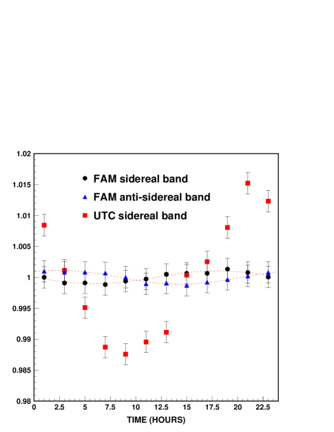
Figure 3: Sidereal modulation for the UTC coverage (red squares) and the sidereal (black circles) and anti-sidereal (blue triangles) sidebands for the FAM coverage. The equal amplitudes sidereal and anti-sidereal sidebands for the FAM coverage are the results of the seasonal modulated solar variation. The dotted lines are fits to the respective sidebands with amplitudes: $(0.10\pm 0.07)$% (sidereal) and $(0.11\pm 0.07)$% (anti-sidereal). We have artificially introduced a shift in the phase of the anti-sidereal band for better visualisation, since this one is practically in phase with the sidereal band.

Figure 3 shows the time distribution used to build the coverage under the FAM hypothesis and the usual scrambling of UTC shower arrival time, when an equatorial dipole of amplitude 2% is present. The dipolar pattern induces a large sidereal contamination into the UTC coverage as can be seen in figure 3. In fact, this is one of the most unfavorable cases for a UTC like coverage map, since it is a pure right ascension distortion, creating a large modulation in the events arrival time distribution. The concept of anti-sidereal time was introduced some time ago by Farley and Storey [18] in order to study long term behaviour of cosmic ray detectors. The authors made use of the fact that a seasonal modulated diurnal variation (both assumed to be harmonic) could be obtained by the interference of sidebands of equal amplitudes and slightly different periods, in which the slightly higher frequency (with respect to a solar frequency) sideband is the well known sidereal band, whereas the slightly lower frequency sideband was called the anti-sidereal component. Therefore, even pure local seasonal and diurnal modulations will give rise to an apparent sidereal anisotropy, but these can then be identified by looking for the associated equal amplitude anti-sidereal sideband. The time distribution of events used in the FAM coverage shows in fact such twin sidebands with fitted amplitudes of about 0.1%. The amplitude of the sidebands is given approximately by the product of the amplitudes of the seasonal and the diurnal components. The fitted amplitudes to the rates of figure 1 imply an expected 6% $\times$ 2% = 0.12% sidereal (anti-sidereal) modulation, which is in pretty good agreement with figure 3. Therefore, by assuming a Julian day $\times$ solar time factorization of the rate, essentially none of the right ascension modulation leaks into the final exposure sky map. It is worth stressing, though, that such a cancellation of sidereal contribution from sky anisotropy can only be achieved by using an integer number of years as already discussed in section 3. We stress as well that unlike Farley and Storey which assume a harmonic form for the seasonal and diurnal modulations, in the FAM method, their analytical forms are extracted directly from the data.

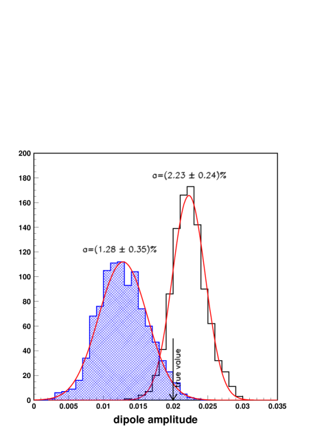
Figure 4: Distribution of reconstructed amplitudes of an equatorial 2% amplitude dipole via the method of reconstruction of pseudo-multipolar coefficients for non-uniform and incomplete sky coverage [22]. Two different coverages: UTC (shaded blue) and FAM, and used as input to the reconstruction are compared. The central values and the standard deviations for the fitted Gaussians are shown on the top of each histogram. Each one of the 1000 samples shown have $5\times 10^{5}$ events.

A more quantitative idea of the bias introduced into the coverage by a simple scrambling of the original arrival times is given in figure 4. The plot shows the distribution of reconstructed amplitudes for 1000 realisations of the 2% equatorial dipole. The reconstruction of dipolar patterns with a full sky observatory was first analysed in [19] with later generalisations to the case of partial sky coverage presented in [20] and [21]. In figure 4, the reconstruction is performed by retrieving the set of multipolar coefficients of the events directions map for a non-uniform and, in this case, even incomplete sky exposure. The central idea of the method is that the pseudo multipolar coefficients obtained with non-uniform partial sky coverage are related to the true ones by a convolution operation whose kernel is a function of the detector window function (the coverage map) [22].

From figure 4 we see a clear underestimation of the dipole amplitude when the reconstruction is done by using the UTC sky map, with the average value ($1.28\pm 0.35$)% being 2$\sigma$ away from the true value. With the FAM coverage, in turn, one is able to retrieve the amplitude within 1$\sigma$. The relative statistical uncertainty of 11% in the amplitude for the FAM case is also smaller than the 27% corresponding to the UTC coverage.

It is interesting to compare these coverage based reconstructions with a coverage independent one. For a pure right ascension (that is sidereal) modulation, it is straightforward to estimate the sidereal amplitude through the power distribution at the sidereal frequency of the arrival time Fourier transform as described in [12]. The reconstruction is done in a two step way. Firstly, the normalised Fourier coefficients of a set of $N$ modified times $\{t_{i}\}$ are calculated at frequency $f$ ($\omega=2\pi f$) as $a(f)=c(f)+is(f)$

$$c(f)=\frac{2}{W}\sum_{i}w_{i}\cos(\omega t_{i}),\quad s(f)=\frac{2}{W}\sum_{i}w_{i}\sin(\omega t_{i})$$ (16)

with $W=\sum_{i}w_{i}$ ($w_{i}=1$), where the sums run all over the $N$ events. An estimation for the annual (diurnal) amplitude $p_{y(d)}=\sqrt{s^{2}(f_{y(d)})+c^{2}(f_{y(d)})}$ and phase $\phi_{y(d)}=\textrm{atan}(s(f_{y(d)}),c(f_{y(d)}))$ is then obtained. Finally, the Fourier amplitudes in (16) are recalculated, now with weights

$$w_{i}=\left[(1+p_{y}\cos(\omega t_{i}-\phi_{y}))\times(1+p_{d}\cos(\omega t_{i}-\phi_{d}))\right]^{-1}$$ (17)

to get the final sidereal amplitude and phase. Such a Fourier analysis, totally independent of the coverage map, gives an amplitude of $(1.6\pm 0.2)$% for the same 2% equatorial dipole, a result somewhere in between the reconstructions through the multipolar coefficients.

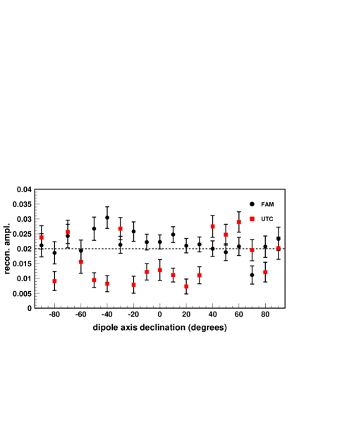
Figure 5: Dipole amplitudes reconstructed through the deconvolution of the multipolar coefficients for non-uniform and incomplete sky coverage [22] as a function of the declination of the dipole axis. FAM (black circles) and UTC (red squares) based coverage maps are compared. The true 2% amplitude is represented by the horizontal dashed line.

A more systematic test of the performance of the FAM and UTC based coverage maps is shown in figure 5, where the reconstructed amplitudes and their associated errors are shown for dipoles with axis at different declinations (and fixed amplitude of 2%). By varying the angle between its axis and the equatorial plane, one changes the amplitude of the induced sidereal variations. One can see that, in average, the amplitude is more accurately retrieved when the FAM coverage map is used as input to the multipolar reconstruction. In the whole range between -90^∘ and 90^∘, the UTC coverage leads to a mean amplitude 2.9$\sigma$ away from the true value, whereas a 1.3$\sigma$ estimation is achieved with the FAM sky map.

6 Conclusions

We have introduced a new method for estimating the exposure sky map of a cosmic ray detector, based on the assumption of factorization of the time behaviour of such a detector into seasonal (represented by the Julian day) and diurnal (represented by the solar time) variations. Such a hypothesis is motivated by the current knowledge on the modulations of the detection rate of large surface arrays caused by weather effects, such as pressure and air temperature, which affects both the longitudinal and lateral developments of particle cascades through the atmosphere. By using an integer number of data taking years, one is able to cancel the sidereal contribution of sky anisotropy to the Julian day and solar time histrograms, allowing to extract the detector time behaviour from the data set itself.

In [17], a model was shown to describe fairly well the yearly and diurnal rate modulations observed in the Auger data set, where the rate is assumed to vary linearly with pressure and air density, with the proportionality coefficients being fitted directly to the number of showers detected by the surface array and to the atmospheric monitoring data taken regularly on site. Using this model, we have shown that possible residual systematic effects caused by the presence of non-factorizable terms into the long term detector behaviour will induce fake large scale anisotropy modulations on the sky no larger than 0.2%, being therefore negligible for a typical 1% desired accuracy into the coverage estimation.

Coverage maps built under the factorization hypothesis were shown to be more suitable when reconstructing dipolar anisotropic patterns through the recovery of its multipolar coefficients, providing amplitudes with a mean systematic shift of 1.3$\sigma$ with respect to the true value as one changes the declination of the dipole axis. The amplitudes reconstructed from a coverage where one simply scrambles the showers arrival times are strongly biased, with values tipically around 3$\sigma$ away from the true values. A coverage independent estimation of the equatorial dipole, such as the one provided by the Fourier analysis of the arrival times and detector running for a 5-year period gives an amplitude somewhere in between the multipolar method with UTC and FAM input coverages, with a systematic underestimation of the amplitude at the $2\sigma$ level.

There are some similarities behind the factorization hypothesis with the analysis performed in [18], but whereas Farley and Storey assume a particular harmonic dependence for both the seasonal and diurnal modulations in order to fit their respective amplitudes, the time distribution used to build the FAM coverage is taken from the data set itself.

References

- [1] N. Hayashida et al. [AGASA Collaboration], Astropart. Phys. 10 (1999) 303 [arXiv:astro-ph/9807045].
- [2] J. Abraham et al. [Pierre Auger Collaboration], Astropart. Phys. 27, 244 (2007) [arXiv:astro-ph/0607382]. E. M. Santos [Pierre Auger Collaboration], to appear in the Proc. 30th ICRC, July 3 - 11, 2007, Merida, Yukatan, Mexico. arXiv:0706.2669 [astro-ph].
- [3] E. Armengaud [Pierre Auger Collaboration], to appear in the Proc. 30th ICRC, July 3 - 11, 2007, Merida, Yukatan, Mexico. arXiv:0706.2640 [astro-ph].
- [4] T. Antoni et al. [The KASCADE Collaboration], Astrophys. J. 604 (2004) 687 [arXiv:astro-ph/0312375].
- [5] M. Ambrosio et al. [MACRO Collaboration], Phys. Rev. D 67 (2003) 042002 [arXiv:astro-ph/0211119].
- [6] K. Munakata et al. [Kamiokande Collaboration], Phys. Rev. D 56 (1997) 23.
- [7] M. Amenomori et al. [The Tibet AS-gamma Collaboration], Phys. Rev. Lett. 93 (2004) 061101 [arXiv:astro-ph/0408187].
- [8] K. Nagashima et al., Il Nuovo Cimento C 12 (1989) 693.
- [9] A. Compton and I.A. Getting, Phys. Rev. 47 (1935) 817.
- [10] M. Amenomori [Tibet AS-gamma Collaboration], Science 314, 439 (2006) [arXiv:astro-ph/0610671].
- [11] The EAS-TOP Collaboration, to appear in the Proc. 30th ICRC, July 3-11, 2007, Merida, Yukatan, Mexico. ibid., Proc. 28th ICRC, Tsukuba, Japan, July 31 - Aug 7, 2003, 183-186.
- [12] P. Billoir and A. Letessier-Selvon, Astropart. Phys. 29, 14 (2008) [arXiv:0706.3705 [astro-ph]].
- [13] J. C. Hamilton [Pierre Auger Collaboration], Proc. 29th ICRC, August 3 -10, 2005, Pune, India, Tata Institute for Fundamental Research, Mumbai, 7 (2005) 63-66. [arXiv:astro-ph/0507517].
- [14] B. Rouillé-d’Orfeuil, “Recherche de sources et d’anisotropies dans le rayonnement cosmique d’ultrahaute énergie au sein de la collaboration AUGER.”, PhD thesis, Université Paris VII, 2007.
- [15] R. W. Clay [Pierre Auger Collaboration], Proc. 28th ICRC, July 31 - August 7, 2003, Tsukuba, Japan. Editors: T. Kajita, Y. Asaoka, A. Kawachi, Y. Matsubara and M. Sasaki, Universal Academy Press, Inc. Tokyo, Japan, HE (2003) 421-424. [arXiv:astro-ph/0308494].
- [16] J. Abraham et al. [Pierre Auger Collaboration], Nucl. Instrum. Meth. A 523, 50 (2004).
- [17] C. Bleve [Pierre Auger Collaboration], to appear in the Proc. 30th ICRC, July 3 - 11, 2007, Merida, Yukatan, Mexico. arXiv:0706.1491 [astro-ph].
- [18] F.J.M. Farley and J.R. Storey, Proc. Phys. Soc., Section A, 67, Issue 11, 996-1004 (1954).
- [19] P. Sommers, Astropart. Phys. 14, 271 (2001) [arXiv:astro-ph/0004016].
- [20] J. Aublin and E. Parizot, Astron. Astrophys. 441 (1) (2005) 407 [arXiv:astro-ph/0504575].
- [21] S. Mollerach and E. Roulet, JCAP 0508, 004 (2005) [arXiv:astro-ph/0504630].
- [22] P. Billoir and O. Deligny, JCAP 0802, 009 (2008) [arXiv:0710.2290 [astro-ph]].