Phase separation of an asymmetric binary fluid mixture confined in a nanoscopic slit pore: Molecular-dynamics simulations

Abstract

As a generic model system of an asymmetric binary fluid mixture, hexadecane dissolved in carbon dioxide is considered, using a coarse-grained bead-spring model for the short polymer, and a simple spherical particle with Lennard-Jones interactions for the carbon dioxide molecules. In previous work, it has been shown that this model reproduces the real phase diagram reasonable well, and also the initial stages of spinodal decomposition in the bulk following a sudden expansion of the system could be studied. Using the parallelized simulation package ESPResSo on a multiprocessor supercomputer, phase separation of thin fluid films confined between parallel walls that are repulsive for both types of molecules are simulated in a rather large system (1356 $\times$ 1356 $\times$ 67.8 Å³, corresponding to about 3.2 million atoms). Following the sudden system expansion, a complicated interplay between phase separation in the directions perpendicular and parallel to the walls is found: in the early stages the hexadecane molecules accumulate mostly in the center of the slit pore, but as the coarsening of the structure in the parallel direction proceeds, the inhomogeneity in the perpendicular direction gets much reduced. Studying then the structure factors and correlation functions at fixed distances from the wall, the densities are essentially not conserved at these distances, and hence the behavior differs strongly from spinodal decomposition in the bulk. Some of the characteristic lengths show a nonmonotonic variation with time, and simple coarsening described by power-law growth is only observed if the domain sizes are much larger than the film thickness.

I INTRODUCTION

Fluids confined in pores with linear dimensions on the $\mu m$ to nm scale find increasing applications and are the subject of many studies, both with respect to their static 1 ; 2 ; 3 ; 4 ; 5 and dynamic 6 ; 7 ; 8 ; 9 ; 10 ; 11 properties. Considering binary fluid mixtures, it is natural to expect that the (enthalpic and entropic) interactions between the pore walls and the fluid particles may differ for both constituents, and then both density and composition develop an interesting inhomogeneity in the direction perpendicular to the pore walls. Of course, already in the bulk the binary fluid may undergo both vapor-liquid unmixing and fluid-fluid phase separation, resulting in complex phase behavior 12 ; 13 . In thin slit pores, phase separation as a thermodynamic phase transition is still possible in the lateral directions parallel to the walls 4 , and due to the possible interplay with wetting phenomena 14 ; 15 ; 16 ; 17 complicated phase diagrams are expected even for strictly symmetric mixtures 4 ; 18 . Particularly interesting, however, is the kinetics of these phase transitions as a function of time $t$ after a quench. For a strictly symmetric binary Lennard-Jones mixture, where one species is strongly attracted by the walls, it has recently been shown by Molecular Dynamics simulations that the lateral phase separation kinetics is characterized by a power-law for the size of the growing domains 19 ; 20 ; 21 ; 22 ; 23 ; 24 ; 25 ; 26 ; 27 ; 28 , $\ell(t)\propto t^{a}$, with 29 ; 30 $a\approx 2/3$ if $\ell(t)$ is in the range of a few Lennard-Jones diameters. While for simple diffusive systems $a=1/3$ both in the bulk 19 and in thin films, at late enough times 31 , the much faster domain growth seen by Das et al. 29 ; 30 for a confined fluid binary mixture may be due to some hydrodynamic mechanisms, but is not in accord with the theoretical expectations 22 ; 23 ; 24 ; 25 ; 26 ; 27 ; 28 . Thus, it is interesting to study the kinetics of phase separation for other models of confined binary mixtures, in order to clarify which features are universal and which features are model specific.

In the present work, we contribute to this problem by studying phase separation for a model of a mixture of hexadecane (C₁₆H${}_{34})$ and carbon dioxide (CO₂). There are several reasons for this particular choice: first of all, supercritical CO₂ is a very important fluid in the chemical industry, useful as a solvent in which various reactions can be carried out 32 ; 33 , particularly applications involving polymers. Thus, the system C₁₆H₃₄ + CO₂ is a prototypical polymer + solvent system 34 . Secondly, a rather simple coarse-grained model for this system has been developed 35 which describes the experimental phase diagram rather accurately. Thirdly, spinodal decomposition in the bulk has already been investigated for this model by extensive simulations 36 . It was found that the system is compatible with a growth according to $\ell(t)\propto t^{1/3}$, when $\ell(t)$ starts to exceed the Lennard-Jones diameters, while at late times a crossover to somewhat faster growth occurs. Limitations due to the finite linear dimensions of the simulation box preclude strong statements on the growth law during the late stages, however.

In Sec. 2, we shall introduce our model and briefly discuss the simulation technique. In Sec. 3, simulation results will be presented and discussed in the light of various theoretical considerations. Sec. 4 contains a summary and outlook to future work.

II MODEL AND SIMULATION DETAILS

II.1 A coarse-grained model for hexadecane + carbon dioxide mixtures

Although hexadecane is a very short polymer only, an all-atom simulation of hexadecane melts would be difficult, since for a simulation study of phase separation kinetics, length scales far beyond the size of a molecule need to be explored, and also large time scales are mandatory 22 ; 25 ; 26 ; 27 ; 28 . Therefore, it is advantageous to use a coarse-grained model. Coarse-graining of polymers is usually done by taking a few chemical monomers (CH₂ or CH₃ at chain ends, in this case) together into effective monomers, ignoring completely torsional potentials 37 ; 38 ; 39 ; 40 . A successful model of this type for C₁₆H₃₄ was proposed by Virnau et al. 35 , incorporating three successive C-C bonds along a chain (plus the corresponding hydrogen atoms) into one effective bead, so that a chain of 5 effective monomers is created. Effective monomers along a chain are bound together via FENE (finitely extensible nonlinear elastic) potentials 41

$$U_{\rm FENE}(r)=-33.75\varepsilon_{\rm pp}\ln[1-(r/R_{\rm pp})^{2}]\quad,\quad R_{\rm pp}=1.5\sigma_{\rm pp}$$ (1)

where $\varepsilon_{\rm pp}$, $\sigma_{\rm pp}$ are parameters of the Lennard-Jones (LJ) potential, that acts between all beads of the polymer chains (bonded as well as non-bonded ones)

$$U(r)=U_{LJ}(r)-U_{LJ}(r_{\rm cut})\quad,\quad U_{LJ}=4\varepsilon_{\alpha\beta}\Big{[}\Big{(}\frac{\sigma_{\alpha\beta}}{r}\Big{)}^{12}-\Big{(}\frac{\sigma_{\alpha\beta}}{r}\Big{)}^{6}\Big{]}\quad,$$ (2)

where a cutoff $r_{\rm cut}=2r_{\rm min}$, $r_{\rm min}=2^{1/6}\sigma_{\alpha\beta}$ is used and the potential is shifted to zero at $r=r_{\rm cut}$ so that $U(r)$ is everywhere continuous, with $U(r\geq r_{\rm cut})=0$. Here $\alpha,\beta=p$ (if the particle is an effective monomer of the chains) or $\alpha,\beta=s$ (if the particle is a solvent molecule). The parameters $\varepsilon_{\rm pp}$, $\sigma_{\rm pp}$ and $\varepsilon_{\rm ss}$, $\sigma_{\rm ss}$ are chosen such that the model reproduces the experimentally known 42 critical temperatures $T_{c}$ and critical densities $\rho_{c}$ for pure C₁₆H₃₄ and pure CO₂, respectively 34 ; 35 . Thus, using 42 $T_{c}=723$K and $\rho_{c}=0.219$g/cm³ has yielded 34 ; 35 (henceforth we omit the index $p$)

$$\varepsilon=5.79\cdot 10^{-21}J,\,\,\sigma=4.52\cdot 10^{-10}m\,,$$ (3)

while the experimental results for CO₂, $T_{c}=304$K and $\rho_{0}=0.464$g/cm³ have yielded 34 ; 35

$$\varepsilon_{\rm ss}=0.726\varepsilon,\quad\sigma_{\rm ss}=0.816\sigma\quad.$$ (4)

With these parameters (Eq. (3) and (4)) the coexistence curves in the temperature-density plane and the vapor pressures at coexistence as well as the interfacial tension between the coexisting phases are reproduced in reasonable agreement with experiment 34 ; 35 . An even better description of CO₂ could be obtained by including the quadrupole-quadrupole interaction 43 , but this is out of consideration in the present context.

The parameters $\varepsilon_{\rm ps}$, $\sigma_{\rm ps}$ for the interactions between CO₂ molecules and effective monomers are described 34 ; 35 using a modified Lorentz-Berthelot mixing rule 44

$$\sigma_{\rm sp}=(\sigma_{\rm ss}+\sigma_{\rm pp})/2\quad,\quad\varepsilon_{\rm sp}=\xi\sqrt{\varepsilon_{\rm ss}\varepsilon_{\rm pp}}\quad,$$ (5)

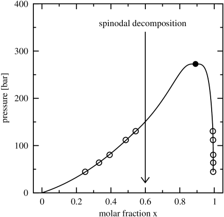
Figure 1: K. Bucior

with 34 ; 35 $\xi=0.886$. While the standard Lorentz-Berthelot mixing rule ($\xi=1$) would yield a phase diagram topology in disagreement with the available experiments 45 , Eq. (5) gives a phase diagram in rough agreement with these experiments 34 ; 35 . In the following, we shall choose $\varepsilon=1$ as unit of temperature (taking Boltzmann’s constant $k_{B}=1$) and $\sigma=1$ as unit of length. Fig. 1 shows an isothermal slice through the phase diagram at reduced temperature $T^{*}\equiv k_{B}T/\varepsilon=1.16$ in the plane of pressure $p$ and molar fraction $x\equiv N^{s}/(N^{s}+N^{p}/5)$ of carbon dioxide, where $N^{s}$ is the number of carbon dioxide molecules and $N^{p}$ the number of effective monomers of hexadecane. As will be described below, we shall simulate pressure-jump experiments where the system suddenly is brought from a state in the one-phase region (the initial state is equilibrated at a density $\rho^{*}_{\rm tot}\equiv\rho\sigma^{3}=0.8$ in the middle of the slit pore, which would correspond to a reduced pressure $p^{*}\equiv p\sigma^{3}/\varepsilon=0.34$ in the bulk system) into the two-phase region by an isotropic increase of the volume available to the particles.

For a system in a thin film geometry, it is also necessary to specify the boundary conditions created by the planar walls confining the thin film. We choose an atomistic description of these walls, putting particles on a regular (and rigid) triangular lattice of lattice spacing $\sigma=1$, in the $(x,y)$ plane at $z=0.01$ and $z=0.99L_{z}$, $z$ being the coordinate in the direction perpendicular to the walls. The interactions between the wall particles $(w)$ and solvent particles or effective monomers are described by the purely repulsive part of the LJ-potential, Eq. (2), using $r_{\rm cut}=r_{\rm min}$ and

$$\varepsilon_{\rm ws}=\varepsilon_{\rm wp}=\varepsilon=1,\quad\sigma_{\rm ws}=\sigma_{\rm wp}=1\quad.$$ (6)

This choice was made to avoid the formation of precursors of wetting layers of one of the species, unlike 29 ; 30 , where an attractive interaction between the walls and one of the species in the binary (A,B) mixture was chosen. We deliberately choose the wall-particle interactions symmetric in the present case, to avoid any strong preference of the wall for one of the components in our case. However, since (unlike to 29 ; 30 ) the present model is not a symmetric mixture in the bulk, we do expect some wall-induced concentration inhomogeneities for the present model as well. As demonstrated recently for the case of colloid-polymer mixtures 46 , an effective attractive interaction due to repulsive walls may arise due to purely entropic origin.

II.2 Simulation method and preparation of the initial state

We study the kinetics of phase separation in thin films of CO₂ + C₁₆H₃₄ mixtures by Molecular Dynamics (MD) methods 47 ; 48 ; 49 . As is well-known, in simple fluids and binary fluid mixtures hydrodynamic interactions are important both for the dynamics of fluctuations near equilibrium 28 ; 50 and for the kinetics of coarsening in the late stages of spinodal decomposition 21 ; 22 ; 23 ; 24 ; 25 ; 26 ; 27 ; 28 . MD simulations (in the microcanonical NVE ensemble where energy $E$ is conserved for fixed number of particles $N$ and fixed volume $V$) include these effects of hydrodynamics implicitly and fully 47 ; 48 ; 49 . In fact, previous studies of phase separation in the bulk have used this method successfully for both simple liquid-vapor phase separation and for studies of unmixing of binary fluid mixtures (see e.g. 51 ; 52 ; 53 ; 54 ; 55 ). We apply for our system the software package ESPResSo, version 1.9.7h, 2005 56 which is particularly suitable for simulation of coarse-grained soft matter systems on parallel computers.

For the integration of Newton’s equation of motion the Velocity Verlet Algorithm 47 ; 48 ; 49 is applied, choosing an integration time step $\delta t=0.002\,\tau$, where the MD time unit here defined as $\tau=\sigma(m/\varepsilon)^{1/2}=1$ corresponds to 500 integration steps. The masses $m$ of CO₂ molecules, effective monomers and wall particles are set for simplicity equal to each other, and time units are chosen such that $m=1$.

The initial state is created by first using a small simulation box $L_{x}\times L_{y}\times L_{z}$ with $L_{x}=L_{y}=20$, $L_{z}=12$ (measured in units of $\sigma$ through this paper) with two repulsive walls at $z=0.01$ and $z=0.99L_{z}$, as described in Sec. 2.1, and periodic boundary conditions in $x$ and $y$-directions. Into this box, hexadecane molecules were inserted, having selfavoiding walk configurations, and the CO₂ particles were inserted at random position, at molar fraction of CO₂ $x=0.6$, such that the initial state reaches a reduced total monomer density of $\rho^{*}_{\rm tot}=0.8$ in the center of the thin film. The CO₂ particles were only allowed to be put at positions outside of a sphere of radius $\sigma=1$ of each bead, to avoid that in the initial state very large repulsive forces occur. Choosing a Langevin thermostat 47 ; 48 ; 49 , the system then is equilibrated at $T^{*}=1.16$ and is replicated three times in $x$ and $y$-directions, to obtain a system with linear dimensions $L_{x}=L_{y}=60$. This 9 times larger system then is equilibrated again, for a time of 300 MD time units ($1.5\times 10^{5}$ MD steps), to remove the effects due to original periodicity at $L_{x}=L_{y}=20$. It was carefully tested that for the chosen conditions (i.e., for a supercritical solution of relatively short chains) such a short re-equilibration time actually was enough. Then the thermostat was switched off, and a Galilei transformation of particle velocities was applied to remove the motion of the center of mass of our model system. This still rather small system, as described above, was only used for testing our simulation and analysis procedures as well as for choosing optimal parameters for the pressure-jump simulations. To obtain the initial state of the full system at the desired dimensions $L_{x}=L_{y}=240$, $L_{z}=12$, the system was replicated again 4 times in $x$- and $y$-direction, and the procedure of equilibration and Galilei transformation, as described above, was repeated again. The structure factor of the system was carefully analyzed to check that any signs of the Bragg peaks (due to the periodic arrangement of the replicas) have disappeared. Then the system was equilibrated further for 400 MD time units ($2\times 10^{5}$ MD steps), before the quench was started. Note that at this stage we have already a total number of $N=589999$ particles, namely 294000 chain segments (i.e., 58800 chains), 88400 solvent particles and 207599 wall particles. Since each CO₂ solvent particle contains 3 atoms, and each C₁₆H₃₄ chain contains 50 atoms, the total number of atoms (if we had an atomistic model) in our system would be 3205200 (not counting the wall atoms).

The pressure-jump quenching experiment has the effect that the system after the sudden quench can take a larger volume, and since the particle numbers always are fixed, this corresponds to a decrease of density. We do not attempt to precisely mimic how the pressure jump is carried out in an actual experiment, but we simply rescale the positions of the centers of mass of hexadecane and carbon dioxide molecules in three directions such that the final dimensions of the simulation box were $L_{x}$=$L_{y}$=300 and $L_{z}=15$. Of course, one must not simply rescale all the coordinates of the effective monomers, since the conformation of an individual C₁₆H₃₄ molecule (bond lengths and positions of the monomers along a chain relative to each other) should not be rescaled but rather stays the same, just the molecules are moved farther apart form each other at lower density. Note that due to Eq. (3) this final size of the box corresponds to $L_{x}=L_{y}=1356$ Å while $L_{z}=67.8$ Å, so the system still is a ultrathin nanoscopic film. Wall particles were removed from the system before the rescaling of CO₂ and C₁₆H₃₄ positions and inserted just after the rescaling procedure, so that the arrangement of the wall particles (and the distances between them) stay exactly the same as before the quench. In addition, we reduce the energy of the system by rescaling the kinetic energy of the particles to ensure that the temperature of the system after the quench becomes very similar to the initial temperature of the equilibrated homogeneous system. Physically the walls confining a thin fluid film would be massive solid walls of a suitable device, of course, and thermostating the walls would have the effect of maintaining constant temperature conditions. Our procedure is meant as a short-cut for such a situation.

The simulation of the system after the quench is performed in the NVE ensemble for 4000 MD time units corresponding to two million MD time steps. For the first 200 MD time units ($10^{5}$ MD steps), 30 runs were performed in parallel, storing configurations after every 10 MD time units. For later times, due to the large computational effort for our system, five systems were propagated and configurations were analyzed for every 100 MD time units only. These simulations were carried out on the multiprocessor system JUMP of the John von Neumann Institute for Computing (NIC) at Jülich, utilizing 16 processors in parallel, and the cluster of the SOFTCOMP EU Network of Excellence, utilizing 4 processors in parallel.

III SIMULATION RESULTS

III.1 Transient segregation between solvent and polymer forming a layered state

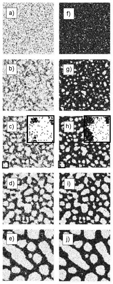
Figure 2: K. Bucior

Fig. 2 shows typical snapshot pictures that illustrate the time evolution of the phase separation process in the thin film. These snapshots show quasi-two-dimensional slices parallel to the wall, the left column being about 3 layers (of total 10) away from the wall, the right column being close to the center of the film (layer 5). Already these pictures show an interesting interplay of phase separation in the directions perpendicular and parallel to the confining walls: in the initial stage, $t=10$ (Figs. 2a, f), the system is still laterally homogeneous, apart from very strongly localized density fluctuations, but there is a strong variation of density across the film: most of the effective monomers are concentrated in the center of the film (Fig. 2f). This observation is still true at $t=50$ (Figs. 2b,g), but now lateral phase separation has clearly started: in the center of the pore (Fig. 2g), the white “holes” mean that CO₂ bubbles with a few hexadecane molecules (i.e., a dilute solution of chains in supercritical CO₂) have formed within the concentrated C₁₆H${}_{34}/$CO₂ solution, while near the walls (Fig. 2b) we rather have ramified clusters of C₁₆H₃₄ molecules in a CO₂-rich fluid. At later times, these structures coarsen ($t$=100, 200) and, at the same time, the difference in density between the center of the thin film and the regions near the walls diminishes. For $t=1000$ (as well as for later times, that are not shown here) the density difference has almost vanished (Figs. 2e, j). What is more important, the regions in the $(x,y)$-plane where the CO₂-C₁₆H₃₄ interfaces occur, are identical in the left and the right snapshot: We can picture the phase separation in the late stages, where the characteristic linear dimensions of the growing CO₂ bubbles in the concentrated C₁₆H₃₄/CO₂ solution in $x,y$- direction are much larger than the film thickness $L_{z}$, simply as a quasi-two-dimensional arrangement of flat cylinders of height $L_{z}$, forming bridges between the two walls. While some of the CO₂-droplets at $t=1000$ still deviate strongly from a circular cross-section in $x,y$-directions, actually an inspection of snapshots at still later times, such as $t=4000$ (not shown here) shows that the droplets in fact do develop towards becoming a circular cross section, thus, minimizing the interfacial area (and energy). Ultimately (at time $t\rightarrow\infty$ in a macroscopically large system in $x,y$-directions) we expect a population of strictly regular cylinders of typical radius $R(t)$ connecting the two walls and with $R(t)$ growing to infinity as well. Unfortunately, for $t=4000$ in our system the number $n(t)$ of cylinders was only $n(t=4000)=8$, implying that the data suffer from very strong finite size effects! In fact, studies of coarsening in simple diffusive models have suggested that finite size effects become important already when the number $n(t)$ of growing domains becomes distinctly smaller than $n(t)=20$ 57 , and hence our data for $t\geq 1000$ clearly suffer from finite size effects, despite the rather large linear dimensions and number of particles in our system. Therefore, there is no point in carrying out our MD simulations for the system dimensions chosen here after longer times.

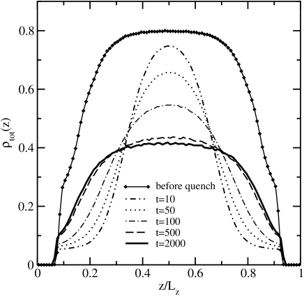
Figure 3: K. Bucior

Fig. 3 shows now the laterally averaged total density of particles which we define as follows

$$\rho_{\rm tot}(z)=(N^{s}_{i}+N^{p}_{i})/V_{i}\quad,$$ (7)

where $N^{s}_{i}$ is the number of solvent (carbon dioxide) molecules in layer $z\equiv z_{i}$ with $z_{i}$ located in the middle of the interval $\Delta z=0.15$; $N^{p}_{i}$ is the number of effective monomers of hexadecane in this layer, and $V_{i}=L_{x}L_{y}\Delta z$ the associated volume of layer $i$. We have tested that the dependence of the profile $\rho_{\rm tot}(z)$ on the width $\Delta z$ of this volume slice $V_{i}$ is not important. Our choice was taken to ensure that fluctuations in $\rho_{\rm tot}(z)$ are small enough but no significant information on the inhomogeneity of the system in $z$-direction is lost. One can see that near both walls there is always a region (of thickness $\approx 0.82\sigma$) essentially free of particles, and then the density both in the initial state and in the final state gradually increases to an almost constant density in the inner part of the film, $\rho_{\rm tot}(z/L_{z}\approx 0.5)\approx 0.8$ before the quench and $\rho_{\rm tot}(z/L_{z}\approx 0.5)\approx 0.4$ during the late stages. However, at early times after the quench, most of the particles accumulate in the center of the film, so the system initially takes a state which shows a phase separation of the liquid-vapor type in the $z$-direction perpendicular to the walls: vapor layers occur close to the walls, and a fluid (where CO₂ and C₁₆H₃₄ are still almost homogeneously mixed) occurs in the center of the film. However, this vertically separated state is unstable against lateral phase separation, in the directions parallel to the walls, as we have already seen from the snapshot pictures in Fig. 2. Thus, in a particular distance $z$ from the walls the density $\rho_{\rm tot}(z)$ approaches its final equilibrium in a non-monotonic fashion as a function of time, e.g., for $z/L_{z}=0.2$ the density decays fast from a rather large value ($\rho_{\rm tot}\approx 0.6$) to a very small value ($\rho_{\rm tot}\approx 0.07$) immediately after the quench, and only when the lateral phase separation starts the density increases again. Note that the two-stage character of the phase separation process, where first a stratified structure forms, with low density in the film center, which then laterally decomposes, is not a consequence of studying a binary mixture, but rather a consequence of purely repulsive wall-particle interactions. In fact, we have checked for pure CO₂ that a similar behavior occurs.

It is also interesting to study the density profiles $\rho_{s}(z)=N_{i}^{s}/V_{i}$ and $\rho_{p}(z)=N^{p}_{i}/V_{i}$ of the solvent particles and the monomers separately, and to define also a profile $c(z)$ of the relative concentration of CO₂,

$$c(z)=\rho_{s}(z)/[\rho_{s}(z)+\rho_{p}(z)]\quad.$$ (8)

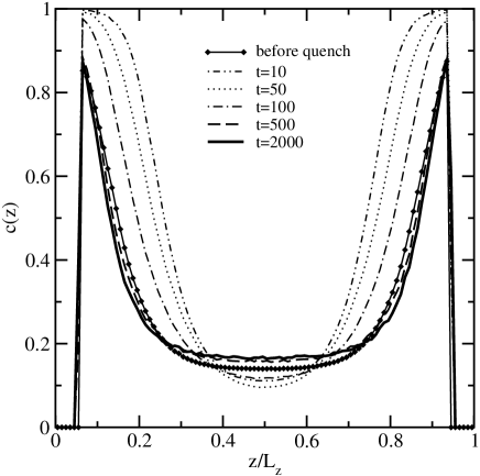
Figure 4: K. Bucior

Fig. 4 displays the latter profile: one can see that despite the fact that we have chosen the same repulsive potential between wall atoms and the monomers or solvent particles, respectively, nevertheless the relative concentration of CO₂ near the walls is strongly enhanced, both in the initial state and during the late stages of phase separation. Actually, the curves for $c(z)$ in the initial state and in the late stages $(t\geq 500)$ almost fall on top of each other! Only in the early times after the quench ($10\leq t\leq 100)$ we do see a much stronger variation of $c(z)$: near the walls almost pure CO₂ phase is reached. So the phase separation clearly proceeds in two stages: induced by the walls, first in the direction perpendicular to the walls a layered structure forms, CO₂ and C₁₆H₃₄ get almost completely segregated, with the polymer film in the center and two CO₂-C₁₆H₃₄ interfaces near $z/L_{z}\approx 0.25$ or 0.75, respectively. However, this state costs far too much (interfacial) energy, and is hence unstable towards lateral phase separation. Both in the initially homogeneous state and in the final state with the “cylindrical” CO₂-domains across the thin film (Fig. 2) we have a strong concentration enhancement of CO₂ near the walls. This enhancement clearly is an entropic effect, from the point of view of configurational entropy polymers tend to avoid the regions close to the walls.

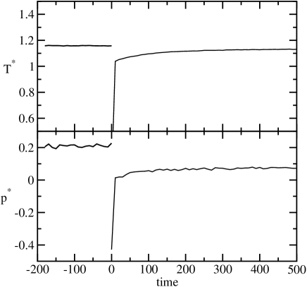
Figure 5: K. Bucior

Of course, for times $t<100$ the system clearly is rather far from equilibrium, and its state is changing rather rapidly. Monitoring the temperature (from the kinetic energy) 47 ; 48 ; 49 and the pressure (using the virial theorem 47 ; 48 ; 49 ) as a function of time after the quench, a distinct but relatively small increase with time in the region $10\leq t\leq 100$ is indeed found (Fig. 5). However, for later times both quantities settle down at constant values, as desired.

III.2 Equal-time structure factors

In experimental studies of phase separation kinetics, most often the equal-time structure factor $S(\vec{q},t)$ is monitored, $\vec{q}$ being the wavevector of a scattering experiment 22 ; 23 ; 24 ; 25 ; 26 ; 27 ; 28 . For a thin film geometry, $\vec{q}$ needs to be oriented in the $(x,y)$-plane, of course, $\vec{q}=\vec{q}_{||}$. Also, due to the inhomogeneity of the system in the $z$-direction (Figs. 3, 4), it is of interest to distinguish in the structure factor from which slice ($z$) the scattering particles contribute to the scattering intensity. Moreover, having two components (which here we symbolically denote as A and B, in order to make contact between our notation and the relevant literature 58 ; 59 ) one must distinguish partial structure factors and those which monitor density and concentration fluctuations. Thus, we define the partial structure factors, resolved with respect to the $z$-coordinate, as follows

$$S_{\alpha\beta}(\vec{q}_{||},z,t)=\frac{1}{N}\sum\limits_{k=1}^{N_{\alpha}}\sum\limits_{\ell=1}^{N_{\beta}}\langle\exp[i\vec{q}\cdot(\vec{r}_{k\ell}(t))]\rangle,$$ (9)

where $\alpha,\beta=A$ or $B$, $\vec{r}_{k\ell}(t)=\vec{r}_{k}(t)-\vec{r}_{\ell}(t)$, and $N_{\alpha}$, $N_{\beta}$ being the numbers of particles of type A or B in the slice at $z$ (i.e., the coordinates $z_{k}(t)$, $z_{\ell}(t)$ of the particles must be in the range $z-\Delta z\leq z_{k}(t)$, $z_{\ell}(t)\leq z+\Delta z$). While ideally one would like to consider the limit $\Delta z\rightarrow 0$, in practice we had to choose a rather larger value of $\Delta z$ (namely $\Delta z=0.75$) in order to get enough statistics.

For fluids $S_{\alpha\beta}(\vec{q}_{||},z,t)$ depends only on the magnitude $q_{||}$ of $\vec{q}_{||}$ and not its direction. Thus, the structure factors monitoring fluctuations of number density $(S_{\rm nn})$ and of concentration $(S_{\rm cc})$ are defined as follow,

$$S_{\rm nn}(q_{||},z,t)=S_{AA}(q_{||},z,t)+2S_{AB}(q_{||},z,t)+S_{BB}(q_{||},z,t)\quad,$$ (10)

$$S_{\rm cc}(q_{||},z,t)=x_{B}^{2}S_{AA}(q_{||},z,t)+x_{A}^{2}S_{BB}(q_{||},z,t)-2x_{A}x_{B}S_{AB}(q_{||},z,t)\,$$ (11)

where $x_{A}=N_{A}/(N_{A}+N_{B})$ and $x_{B}=N_{B}/(N_{A}+N_{B})$ are the relative concentrations of A(B) particles in the slice centered at $z$. To simplify the notation in the following, the index $||$ from $q_{||}$ will be omitted.

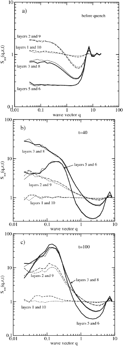
Figure 6: K. Bucior

Note that due to the motion of particles in the $z$-direction, $N_{A}$ and $N_{B}$ are not conserved for a selected layer; in particular, during the early stages of phase separation, $x_{A}$ and $x_{B}$ change strongly with time. As an example, Fig. 6 presents $S_{\rm nn}(q,z,t)$ as a function of wavenumber $q$ for different choices of $z$ and three times: before the quench (a), at $t=40$ (b) and $t=100$ (c) after the quench. The values of $z$ shown in the figure are symmetric around the center of the film, which occurs at $(L_{z}/2)$, and therefore pairs of curves should superpose, apart from statistical errors. We see that this symmetry indeed is rather well satisfied (e.g., the curves for the layers 5 and 6 are indistinguishable from each other in the scale shown in Fig. 6c), and hence the statistical errors of our data indeed are rather well under control. One can see a peak near $q=2\pi$ which changes relatively little with time: this peak and the structure at still larger $q$ reflect the local packing of particles in a dense fluid. Apart from the values of $z$ very close to the walls (e.g., for layers 1 and 10, where almost no particles occur, as the density profiles $\rho(z,t)$ in Fig. 3 show), all curves exhibit a minimum somewhere in the region $2\leq q\leq 4$, while for smaller $q$, the structure factor $S_{\rm nn}(q,z,t)$ increases again. In equilibrium, the maximum of the structure factor occurs for $q\rightarrow 0$ (Fig. 6a), as expected, while after the quench for large enough times, $S_{\rm nn}(q,z,t)$ exhibits a well-defined maximum for small $q$ (Fig. 6c): this small-angle scattering is the “hall mark” of spinodal decomposition. However, close to the walls (i.e., for layers 2, 3, 8 and 9 centered at $z=2.25$, $3.75$, $11.25$ and $z=12.75$, respectively, in Fig. 6b) the scattering intensity for small $q$ does not seem to decrease again, and so the maximum is much less pronounced. Indeed, this range of $z$ clearly exhibits a lack of conservation of the density, due to the rapid change of the total density $\rho(z,t)$ in this regime of times (cf. Fig. 3).

The analysis of $S_{\rm cc}(q,z,t)$ gives a similar picture, and hence is not shown here. We rather try to use both $S_{\rm nn}(q,z,t)$ and $S_{\rm cc}(q,z,t)$ to extract characteristic lengths $R(t)$ by taking suitable ratios of moments 22 . We define $R_{1}(z,t)$ from $S_{\rm nn}(q,z,t)$

$$R_{1}(z,t)=2\pi\sum\limits_{q=0}^{q=q_{\rm cut}}S_{\rm nn}(q,z,t)/\sum\limits_{q=0}^{q=q_{\rm cut}}qS_{\rm nn}(q,z,t)\quad,$$ (12)

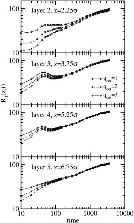
Figure 7: K. Bucior

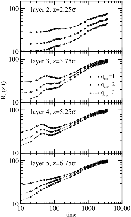
Figure 8: K. Bucior

and similarly for $R_{2}(z,t)$ from $S_{\rm cc}(q,z,t)$. The resulting data are shown in Figs. 7 and 8 for different choices of $z$ and different values for the cutoff $q_{\rm cut}$.

Data for $1\leq t\leq 10$ were not included, since at such extremely short times after the quench both pressure and temperature still are rather strongly time-dependent, the system is very far from equilibrium in all respects, and a discussion of the evolution of the system in terms of the concepts on coarsening 22 ; 23 ; 24 ; 25 ; 26 ; 27 ; 28 would be rather misleading. Also the behavior in the next decade, $10\leq t\leq 100$, is difficult to interpret: we see an unusually strong dependence of both $R_{1}(z,t)$ and $R_{2}(z,t)$ on the cutoff $q_{\rm cut}$, and for some values of $z$ there occurs a slight maximum at about $30\leq t\leq 60$. This behavior can be attributed to the special interplay between phase separation in the directions parallel and perpendicular to the walls (Figs. 2-4). Since the redistribution of both density (Fig. 3) and relative concentration (Fig. 4) between different $z$ is so pronounced during this range of times, the time evolution for a given value of $z$ is similar to the time evolution of a system whose order parameter is not conserved. In the thin film as a whole, however, both particle numbers are conserved; hence, the density and concentration are conserved variables, when we consider the total film. Only for times $t=500$ or larger the profiles of density $\rho(z)$ and concentration $c(z)$ are practically independent of time, and then in a particular layer (i.e., particular value of $z$) the order parameters behave as if they were strictly conserved. Gratifyingly, in the time region from 200$\leq t\leq 2000$ the data for $R_{1}(z,t)$ and $R_{2}(z,t)$ show indeed a much more standard behavior, being essentially independent from the cutoff $q_{\rm cut}$, and almost independent of $z$, showing that now a well-defined unique length scale exists in the system. Figs. 7, 8 reveal that in this range of times we almost find straight lines at the log-log plots, with a slope slightly below 1/3. For $t\geq 2000$ the curves even get slightly flatter, so the growth gets slower; we attribute this effect to the onset of finite size effects. An important finding of our study, however, is that we do not see any evidence for the anomalous law $\ell(t)\propto t^{2/3}$ found by Das et al. 29 ; 30 in a symmetric mixture confined in thin film geometry. It remains to be understood whether this different coarsening behavior is primarily due to the lack of symmetry between phase separating species in our system or due to different boundary conditions at the walls.

III.3 Equal-time correlation functions in real space

In the context of simulations, it has some practical advantages to extract characteristic lengths from the equal-time correlation functions in real space 60 rather than using the structure factors. In fact, also the result for a length $\ell(t)$ growing as $\ell(t)\propto t^{2/3}$ was extracted from such a real-space analysis 29 ; 30 . Thus, it is of interest to study real-space correlations in the present context, too, to check whether the findings of Figs. 7 and  8 are corroborated.

We define a normalized pair correlation function $G(r,z,t)$ as

$$G(r,z,t)=\frac{g(r,z,t)-1}{\tilde{g}(r=0,z,t)-1}\quad,$$ (13)

where $g(r,z,t)$ in the equal-time radial distribution function for effective monomers of hexadecane in a slice $z$ of width $2\Delta z=1.5\sigma$ at the time $t$. Here, the distance $r=|\vec{r}_{k}(t)-\vec{r}_{\ell}(t)|$ and the coordinates $z_{k}(t)$, $z_{\ell}(t)$ of the particles labeled as $k$ and $\ell$ are restricted to this slice, as in Eq. (9). The value of $\tilde{g}(r=0,z,t)$, which is used to normalize $G(r,z,t)$, we obtain by extrapolating $g(r,z,t)$ from the region $r>4\sigma$ to $r=0$ as described below, thus ignoring the local packing effects, which are present in the radial distribution function at short distances.

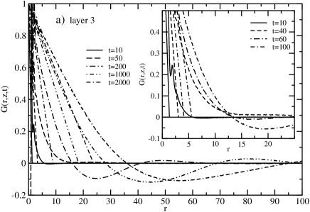
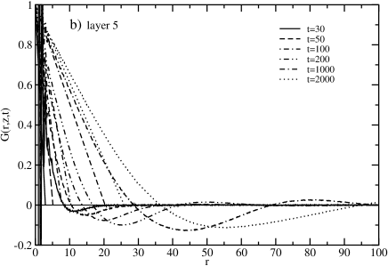
Figure 9: K. Bucior

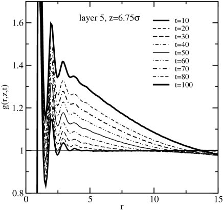
Figure 10: K. Bucior

Fig. 9 shows such data for the layer 3 ($z=3.75\sigma$) (a) and the layer 5 ($z=6.75\sigma$) (b). While in the center of the film (layer 5) the curves intersect the abscissa, and hence one could follow the traditional method 27 ; 30 to define a characteristic domain linear dimension $\ell(t)$ from the first zero crossing of $G(r,z,t)$, this method clearly does not work in slices close to the walls: e.g., for $z=3.75\sigma$ and time $t=40$ (shown in the inset of Fig. 9a) we rather see a continuous decay towards the abscissa with a very flat minimum at $r\approx 18\sigma$ instead of a clearly identifiable crossing of the abscissa. Thus, we tried heuristically an alternative way to extract a length $\ell(t)$, by fitting a straight line to $G(r,z,t)$ in the regime $0.6\leq G(r,z,t)\leq 1$. The zero-crossing of these straight lines would allow to identify a length $\ell(t)$ for all values of $z$. However, this method also is doubtful, particularly for times $t\leq 100$, since there the curves for $G(r,z,t)$ show strong oscillations for small $r$. These oscillations are not due to bad statistics, but simply reflect the liquid short range order: oscillatory variation of $g(r,z,t)$ due to the packing of particles in the nearest neighbor shell, next nearest neighbor shell, third nearest neighbor shell, etc., around a particle 58 . This short range order needs to be disentangled from the growth of a length scale due to phase separation (Fig. 10). Only when $g(r)$ is distinctly nonzero for $r\geq 4\sigma$, the growing length scale can be identified; therefore, very short times (such as $t=20$) obviously must be discarded. However, in the regime $r\geq 4\sigma$ and $t\leq 100$, $g(r,z,t)$ exhibits also clear curvature, and hence any straight line fit prone to large systematic errors. Therefore, we choose the ad hoc form

$$y(r,z,t)=1+a(z,t)\exp[-r/\tilde{l}(z,t)]+b(z,t)$$ (14)

to smooth our data for $g(r,z,t)$ using $a(z,t)$, $\tilde{l}(z,t)$, and $b(z,t)$ as fit parameters; $b(z,t)$ is negative when a zero crossing (i.e., $g(r,z,t)-1=0$ at $r>4\sigma$) occurs and is positive otherwise. This fit-function is used in the range $r>4\sigma$ and $g(r,z,t)>1.01$ but actually provides a good representation of the actual data down to and below the first-zero crossing for those values of $z$ and $t$ where such a zero crossing occurs. Also, this function is used to extrapolated from the region $r>4\sigma$ to $r=0$ to obtain the normalization constant $\tilde{g}(r=0,z,t)=1+a(z,t)+b(z,t)$ for Eq. (13). From the first-order Taylor expansion of Eq. (14) we obtain an approximation to $G(r,z,t)$

$$G(r,z,t)\approx\frac{a(z,t)[1-r/\tilde{l}(z,t)]+b(z,t)}{a(z,t)+b(z,t)}=1-r/l(z,t)$$ (15)

from which we can also define a characteristic length $l(z,t)=\tilde{l}(z,t)(a(z,t)+b(z,t))/a(z,t)$ as a value of $r$ at the intersection of a line given by Eq. (15) with the axis $G=0$.

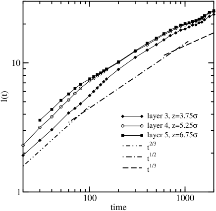
Figure 11: K. Bucior

Fig. 11 shows the time evolution of the characteristic length $\ell(z,t)$ extracted in this way for three choices of $z$. While for $t<100$, where $\ell(z,t)$ is only of the order of a few $\sigma$, indeed the data seem to be compatible with a behavior $\ell(z,t)\propto t^{2/3}$ as observed by Das et al. 29 , for the decade $100\leq t\leq 1000$ the data seem to be compatible with $\ell(z,t)\propto t^{1/2}$ showing a crossover to $\ell(z,t)\propto t^{1/3}$ at later time. For $t\geq 1000$, a crossover to a still slower growth is evident in our simulations, which is however strongly affected by finite size effects, since the number of growing (cylinder-shaped) domains is already rather small. Note that this implies that finite size effects already set in for $\ell(z,t)\approx 20\sigma$, so despite our large system ($300\sigma\times 300\sigma$) we cannot follow the kinetics of spinodal decomposition for a large enough range of times in order to make significant statements on the asymptotic power law growth! Much larger systems need to be simulated for this purpose.

IV CONCLUSIONS

In this work, we have presented computer simulations of spinodal decomposition of a coarse-grained model for a compressible binary fluid mixture, which roughly describes hexadecane dissolved in supercritical carbon dioxide. This system has a very asymmetric phase diagram in the plane of variables pressure and molar fraction (Fig. 1), and the pressure-jump considered in the present work is strongly off-critical: the number of CO₂ molecules is 88400 while the number of C₁₆H₃₄ chains is 58800 (leading to 294000 effective segments). We find that the phase separation is a two-step process: in the first step, there is a strong segregation between solvent and polymer leading to a layered structure, with solvent rich layers adjacent to the walls, and a polymer-rich ultrathin polymer film “sandwiched” in between. This stratified structure, however, is unstable: the free-standing polymer film in the center of the slit pore breaks up, CO₂-rich bubbles form, and finally a pattern develops with cylinder-shaped CO₂-rich domains, the radius of which grows with a $\ell(t)\propto t^{1/3}$ law (at the latest stages accessible to our simulation, as long as finite size effects are still negligible). For the earlier stages of phase separation, where a strong coupling between the phase separation in perpendicular and parallel directions (with respect to the walls) occurs, we conclude that a description of the structure in terms of power laws of characteristic linear dimensions is somewhat misleading, since characteristic lengths extracted from the structure factor and from the pair correlation function are quite incompatible with each other. We suggest that there is no simple scaling behavior in this regime. Note that although we have chosen the potential between wall particles and solvent particles identical to the potential between wall particles and effective monomers, both in the initial and final stages of phase separation there is significant enrichment of CO₂ near the walls, although our snapshot pictures (resolved as function of $z$ and $t$ in Fig. 2) indicated that the data still belong to an incomplete wetting regime.

Thus, it would be interesting to have a more detailed theoretical understanding from analytical theory for phase separation with two coupled order parameters (density and concentration, in our case). Additional simulations would be valuable where wall-particle interactions are chosen such that a strictly “neutral wall” situation is achieved, where no surface enrichment occurs, and hence the pure confinement effect on phase separation (not disturbed by the formation of precursors of wetting layers) could be studied. Also, it would be clearly worthwhile to study more systematically how the phase separation kinetics depends on slit thickness, composition of the mixture, and quench depth. We did some preliminary runs at one different quench depth in which the system volume was increased by factor 1.73 instead of 1.95 discussed in our paper and found a rather similar behavior. However, significantly different behavior is expected for shallow quenches through the critical point, since the correlation length of density and concentration fluctuations can exceed the slit thickness, and formation of a stratified structure is not expected. Finally, in order to get rid of finite size effects, simulations with billions of particles on massively parallel supercomputers would be required. However, such detailed and computationaly extensive studies would be a very challenging task for presently available computer resources and itself could be a topic for forecoming papers. We also hope the present work will stimulate more work on the kinetics of phase separation in nanoscopic confinement such as very thin channels.

Acknowledgements: One of us (K. Bucior) acknowledges support via an Alexander von Humboldt-Fellowship. We are grateful to the J. von Neumann Institute for Computing (NIC) for access to the JUMP multiprocessor and to the EU Network of Excellence for access to the SOFTCOMP Cluster at Jülich Supercomputing Centre (JSC). Helpful discussions with S.K. Das, J. Horbach, M. Müller, W. Paul and P. Virnau are acknowledged. We also thank T. Stühn for his advice with the ESPResSo software.

FIGURE CAPTION

FIG.1. Isothermal slice through the binary phase diagram of the present model for CO₂ + C₁₆H₃₄ mixtures at $T=486.2$K (reduced temperature $T^{*}=1.16$) in the bulk, using the pressure $p$ and the molar fraction $x$ of CO₂ as variables. The coexistence curve encloses a two-phase coexistence region containing a polymer-rich phase (left) and a supercritical CO₂ vapor (near $x=1$, right). The simulations of quenching experiments discussed in the present paper are done for $x=0.6$. This phase diagram is taken from the results of Ref. 35 .

FIG.2. Snapshot picture showing the structure formation after the quench for $L_{x}\times L_{y}=300\sigma$ slices of width $1.5\sigma$ centered at $z=3.75\sigma$ (a-e) and at $z=6.75\sigma$ (f-j). Snapshots are presented at times $t=10$ (a, f), $50$ (b, g), $100$ (c, h), $200$ (d, i) and $1000$ (e, j). The insets in snapshots (c) and (h) illustrate the enlarged regions in the left-bottom corner of size $30\sigma\times 30\sigma$ (marked by rectangles): the gray spheres correspond to the supercritical solvent molecules, and the black ones represent the chain molecules.

FIG.3. Total density profile $\rho_{\rm tot}(z)$ (laterally averaged in the thin film) plotted vs. position across the slit pore $z/L_{z}$ for the initial state before the quench ($L_{z}=12\sigma$, $L_{x}=L_{y}=240\sigma$), and for different stages of phase separation ($L_{z}=15\sigma$, $L_{x}=L_{y}=300\sigma$). The curves are shown at different times after the quench, as indicated.

FIG.4. Relative concentration profile $c(z)$ of the solvent laterally averaged in the thin film plotted vs. position across the slit pore $z/L_{z}$ for the same times and the system dimensions as shown in Fig. 3.

FIG.5. Time evolution of the reduced temperature $T^{*}$ (top) and the reduced pressure $p^{*}$ (bottom) before and after the quench. The time of the quench is at $t=0$.

FIG.6. Density-density structure factor $S_{\rm nn}(q,z,t)$ in the initial state after equilibration (just before the quench) for the system of the linear dimensions $L_{x}=L_{y}=240\sigma$, $L_{z}=12\sigma$ (a), and after the quench at times $t=40$ (b) and $t=100$ (c) for the system dimensions $L_{x}=L_{y}=300\sigma$, $L_{z}=15\sigma$. Various choices of $z$ are included, as indicated in the figure. In case (a), an average over 130 configurations was performed, while in cases (b) and (c), 30 configurations were averaged over. Note: the two curves for layers 5 and 6 (in the middle of the slit pore) cannot be distinguished on the scale shown in figure (c). In all cases, the film was divided into 10 slices of width $2\Delta z=L_{z}/10$.

FIG.7. Log-log plot of the characteristic domain size $R_{1}(z,t)$ (calculated from the density-density structure factor $S_{\rm nn}$ shown in Fig. 6) vs. time for four choices of $z$, as indicated in the figure, and three plausible choices of the cutoff for the wave vector: $q_{\rm cut}=1,2$, or $3$, respectively.

FIG.8. Log-log plot of the characteristic domain size $R_{2}(z,t)$ (calculated from the concentration-concentration structure factor $S_{\rm cc}$) vs. time for four choices of $z$, as indicated in the figure, and three plausible choices of the cutoff for the wave vector: $q_{\rm cut}=1,2$, or $3$, respectively.

FIG.9. The real-space normalized pair correlation function $G(r,z,t)$ [Eq. (13)] vs. distance $r$ for $z=3.75\sigma$ (a) and $z=6.75\sigma$ (b) at various times, as indicated in the figure. The inset in part (a) shows a magnification of the region near the origin for early stage of spinodal decomposition. Note, that the curve for $t=40$ exhibits a very flat local minimum near $r\approx 18\sigma$, which prohibits using the first-zero crossing of $G(r,z,t)$ to measure the characteristic domain size in this range of the time. Straight lines illustrate fits to estimate the characteristic domain length scale $l(z,t)$ from an effective initial slope of these curves at $r=0$ using Eq. (15).

FIG.10. Plot of the radial distribution function $g(r,z,t)$ for the middle layer ($z=6.75\sigma$) vs. distance $r$ for various times, as indicated.

FIG.11. Log-log plot of characteristic domain linear dimension vs. time calculated in three layers of thickness $\Delta z=1.5\sigma$ parallel to the walls, centered at $z=3.75\sigma$, $5.25\sigma$ and $z=6.75\sigma$, respectively. The domain size shown here is defined in the text by Eq. (15). Straight lines are the guide for eyes illustrating the power laws $\ell(t)\propto t^{1/3}$ (dashed line), $\ell(t)\propto t^{1/2}$ (dashed-dotted line) and $\ell(t)\propto t^{2/3}$ (dashed-double dotted line), respectively.

References

- (1) C.A. Croxton (ed.) Fluid Interfacial Phenomena (Wiley, New York 1995)
- (2) D. Henderson (ed.) Fundamentals of Inhomogeneous Fluids (M. Dekker, New York, 1992)
- (3) L.D. Gelb, K.E. Gubbins, R. Radhakrishnan, and M. Sliwinska-Bartkowiak, Rep. Progr. Phys. 62, 1573 (1999)
- (4) K. Binder, D.P. Landau, and M. Müller, J. Stat. Phys. 110, 1411 (2003)
- (5) M. Schoen and S.H.L. Klapp, Nanoconfined Fluids: Soft Matter Between Two and Three Dimensions, Revs. Comput. Chem. 24 (Wiley-VCH, Hoboken, 2007)
- (6) K. Binder, J. Non-Equilib. Thermodyn. 23, 1(1998)
- (7) B. Frick, R. Zorn, and H. Büttner (eds.) International Workshop on Dynamics in Confinement, J. Phys. IV, 10 (2000).
- (8) B. Frick, M. Koza, and R. Zorn (eds.) 2nd International Workshop on Dynamics in Confinement, Eur. Phys. JE 12, Nr. 1 (2003)
- (9) A. Meller, J. Phys.: Condens. Matter 15, R581 (2003)
- (10) T.M. Squires and S.R. Quake, Rev. Mod. Phys. 77, 977 (2005)
- (11) M. Koza, B. Frick, and R. Zorn (eds.) 3rd Intermat-Workshop on Dynamics in Confinement, Eur. Phys. J.ST 141 (2007).
- (12) P. van Konyenburg and R.L. Scott, Philos. Trans. Soc. London Series A298, 495 (1980)
- (13) J.S. Rowlinson and F.L. Swinton, Liquids and Liquid Mixtures (Butterworths, London, 1982)
- (14) P.G. de Gennes, Rev. Mod. Phys. 57, 827 (1985)
- (15) D.E. Sullivan and M.M. Telo da Gama, in Ref. 1, Chap. 2
- (16) S. Dietrich, in Phase Transitions and Critical Phenomena, Vol. 12, edited by C. Domb and J.L. Lebowitz (Academic Press, London, 1988), Chap. 1
- (17) D. Bonn and D. Ross, Rep. Progr. Phys. 64, 1085 (2001)
- (18) M. Müller and K. Binder, J. Phys.: Condens. Matter 17, S333 (2005)
- (19) I.M. Lifshitz and V.V. Slyozov, J. Phys. Chem. Solids 19, 35 (1961)
- (20) K. Binder and D. Stauffer, Phys. Rev. Lett. 33, 1006 (1974); K. Binder, Phys. Rev. B15, 4425 (1977)
- (21) E.D. Siggia, Phys. Rev. A20, 595 (1979)
- (22) J.D. Gunton, M. San Miguel, and P.S. Sahni, in Phase Transitions and Critical Phenomena, Vol. 8, edited by C. Domb and J.L. Lebowitz (Academic Press, London, 1983), Chap. 3
- (23) M. San Miguel, M. Grant and J.D. Gunton, Phys. Rev. A31, 1001 (1985)
- (24) H. Furukawa, Phys. Rev. A31, 1103 (1985); ibid, 36, 2288 (1987)
- (25) Dynamics of Ordering Processes in Condensed Matter, edited by S. Komura and H. Furukawa (Plenum Press, New York, 1988)
- (26) A.J. Bray, Adv. Phys. 43, 357 (1994)
- (27) K. Binder and P. Fratzl, in Phase Transformation in Materials, edited by G. Kostorz (Wiley-VCH, Weinheim, 2001) p. 409
- (28) A. Onuki, Phase Transition Dynamics (Cambridge Univ. Press, England, 2002)
- (29) S.K. Das, S. Puri, J. Horbach, and K. Binder, Phys. Rev. Lett. 96, 016107 (2006)
- (30) S.K. Das, S. Puri, J. Horbach, and K. Binder, Phys. Rev. E73, 031604 (2006)
- (31) S.K. Das, S. Puri, J. Horbach, and K. Binder, Phys. Rev. E72, 061603 (2005)
- (32) E. Kiran and J.M.H. Levelt-Sengers (eds.) Supercritical Fluids (Kluwer, Dordrecht, 1994)
- (33) M.F. Kemmere and Th. Meyer (eds.) Supercritical Carbon Dioxide in Polymer Reaction Engineering (Wiley-VCH, Weinheim, 2005)
- (34) K. Binder, M. Müller, P. Virnau, L.G. MacDowell, Adv. Polym. Sci. 173, 1 (2005)
- (35) P. Virnau, M. Müller, L.G. MacDowell, and K. Binder, Comp. Phys. Commun. 147, 378 (2002); J. Chem. Phys. 121, 2169 (2004)
- (36) L. Yelash, P. Virnau, W. Paul, K. Binder and M. Müller, preprint
- (37) K. Binder (ed.) Monte Carlo and Molecular Dynamics Simulations in Polymer Science (Oxford Univ. Press, Oxford, 1995)
- (38) J. Baschnagel, K. Binder, P. Doruker, A.A. Gusev, O. Hahn, K. Kremer, W.L. Mattice, F. Müller-Plathe, M. Murat, W. Paul, S. Santos, U.W. Suter, and V. Tries, Adv. Polym. Sci. 152, 41 (2000)
- (39) M. Kotelyanskii and D.N. Theodorou (Eds.) Computer Simulation Methods of Polymers (M. Dekker, New York, 2004)
- (40) G. Voth (ed.) Coarse-Graining of Condensed Phase and Biomolecular Systems (Taylor & Francis, in press)
- (41) K. Kremer and G.S. Grest, J. Chem. Phys. 92, 5057 (1990)
- (42) NIST website: http://webbook.nist.gov/chemistry/
- (43) B.M. Mognetti, L. Yelash, P. Virnau, W. Paul, K. Binder, M. Müller, and L.G. MacDowell, J. Chem. Phys. (in press)
- (44) G.C. Maitland, M. Rigby, E.B. Smith, and W.A. Wakeham, Intermolecular Forces (Clarendon Press, Oxford, 1981)
- (45) G. Schneider, Z. Alwani, W. Heim, E. Horvath, and E.U. Franck, Chem. Ing. Techn. 39, 649 (1967); C.T. Amon, R.J. Martin, and R. Kobayashi, Fluid Phase Equilibria 31, 89 (1986)
- (46) R.L.C. Vink, K. Binder, and J. Horbach, Phys. Rev. E73, 056118 (2006); R.L.C. Vink, A. De Virgiliis, J. Horbach, and K. Binder, Phys. Rev. E74, 031601 (2006)
- (47) M.P. Allen and D.J. Tildesley, Computer Simulation of Liquids (Clarendon Press, Oxford, 1987)
- (48) D.C. Rapaport, The Art of Molecular Dynamics Simulation (Cambridge Univ. Press, Cambridge, 1995)
- (49) K. Binder and C. Ciccotti (eds.) Monte Carlo and Molecular Dynamics of Condensed Matter (Italian Physical Society, Bologna, 1996)
- (50) P.C. Hohenberg and B.I. Halperin, Rev. Mod. Phys. 49, 435 (1977)
- (51) S.W. Koch, R.C. Desai, and F.F. Abraham, Phys. Rev. A27, 2152 (1983)
- (52) W.J. Ma, A. Maritan, J.R. Banavar, and J. Koplik, Phys. Rev. A45, R5347 (1992)
- (53) R. Yamamoto and K. Nakanishi, Phys. Rev. B49, 14958 (1994); ibid, B51, 2715 (1995)
- (54) M. Laradji, S. Toxvaerd, and O.G. Mouritsen, Phys. Rev. Lett. 77, 2253, (1996); Physica A239, 404 (1997)
- (55) H. Kabrede and R. Hentschke, Physica A, 361, 485 (2005)
- (56) This package is available at the homepage http://www.espresso.mpg.de; for a description see also H.-J. Limbach, A. Arnold, B.A. Mann, and C. Holm, Comp. Phys. Commun. 174, 704 (2006)
- (57) D.W. Heermann, L. Yiue, and K. Binder, Physica A, 230, 132 (1996)
- (58) J.P. Hansen and I.R. McDonald, Theory of Simple Liquids (Academic Press, San Diego, 1986)
- (59) A.B. Bhatia and D.E. Thornton, Phys. Rev. B2, 3004 (1970)
- (60) J.G. Amar, F.E. Sullivan, and R.D. Mountain, Phys. Rev. B37, 196 (1988)