Time- and Spacelike Nucleon Electromagnetic Form Factors beyond Relativistic Constituent Quark Models

Abstract

For the first time, a phenomenological analysis of the experimental electromagnetic form factors of the nucleon, both in the timelike and spacelike regions, is performed by taking into account the effects of nonvalence components in the nucleon state, within a light-front framework. Our model, based on suitable Ansatzes for the nucleon Bethe-Salpeter amplitude and a microscopic version of the well-known Vector Meson Dominance model, has only four adjusted parameters (determined by the spacelike data with $\chi^{2}/datum\sim 1.7$), and yields a nice description of the experimental electromagnetic form factors in the physical region in the range $-30~{}(GeV/c)^{2}~{}<~{}q^{2}~{}<20~{}(GeV/c)^{2}$, except for the neutron one in the timelike region. Valuable information can be gained in the timelike region on possible missing Vector Mesons around $q^{2}\sim 4.5~{}(GeV/c)^{2}$ and $q^{2}\sim 8.0~{}(GeV/c)^{2}$.

In recent years there has been a renewed interest in the investigation of nucleon electromagnetic form factors (FF), given an unexpected discrepancy between experimental data for the spacelike (SL) ratio $\mu^{p}~{}G^{p}_{E}(q^{2})/G^{p}_{M}(q^{2})$ extracted by using: i) the Rosenbluth separation method (see Ref. [1] for recent measurements) and ii) the polarization transfer technique adopted in experiments carried out at TJLAB [2]. Indeed in the SL region (where the squared four-momentum transfer becomes negative, i.e. $q^{2}=\omega^{2}-|{\bf q}|^{2}~{}\leq~{}0$), data obtained by the Rosenbluth separation follow the dipole law, while, surprisingly, data from the polarization transfer technique decrease faster than the dipole law for $Q^{2}=-q^{2}>1~{}(GeV/c)^{2}$. This experimental puzzle has not yet been completely explained, although both two-photon exchange processes [3] and higher-order radiative corrections [4] appear relevant for its solution.

Furthermore, the timelike (TL) region calls for both experimental and theoretical investigations (in particular for the neutron !), since the ratio, $R$, between experimental neutron and proton form factors, beyond the threshold $q^{2}=4M^{2}_{N}$ (with $M_{N}$ the nucleon mass), turns out to be greater than one [5], while naive expectations from perturbative QCD (see, e.g. [6]) yield $R\sim|e_{d}/e_{u}|=0.5$. A deeper understanding of all these experimental issues could open new windows in the investigation of the nucleon internal structure, also elucidating the role of small components in the nucleon state, (see, e.g., [7] for the possible influence of the above mentioned SL puzzle on the nucleon shape studies).

Within the light-front dynamics [8, 9], we successfully reproduced the pion experimental FF in the interval $-10~{}(GeV/c)^{2}\leq q^{2}\leq 10~{}(GeV/c)^{2}$ [10], namely both in the SL and TL regions, by introducing components of the pion state beyond the valence one. Aim of this letter is the generalization of our approach to the nucleon, presenting for the first time within the light-front dynamics a unified, direct calculation of both SL and TL nucleon FF (see, also [11] for preliminary results with a slightly different model). In particular, the role of the contribution due to the $q\bar{q}$-pair, created by the incoming virtual photon, turns out to be essential as in the pion case. Our approach shares many ingredients with the model of Ref. [12], but it exhibits distinct features, like i) the choice of a reference frame with the plus component of the momentum transfer $q^{+}=q^{0}+q_{z}\neq 0$ [13], allowing a unified analysis of SL and TL regions (see Figs. 2 and 2 for a diagrammatic illustration), and ii) the gauge-invariant dressing of the quark-photon vertex through a microscopic Vector Meson Model (VMD) [10].

Nucleon FF, that enter in the macroscopic description of the em current operator, $I^{\mu}(q^{2})$, are calculated in a reference frame where ${\bf q}_{\perp}={\bf P_{N}}_{\perp}=0$ and $q^{+}=\sqrt{|q^{2}|}$. In the SL region, where $q^{\mu}={P^{\prime}}_{N}^{\mu}~{}-~{}P_{N}^{\mu}$ (with $P_{N}$ and $P_{N}^{\prime}$ the initial and final nucleon four-momenta, respectively) and $q^{2}\leq 0$, the nucleon Sachs FF are given by

$$G_{E}^{N}(q^{2})={1\over 2}Tr\left\{{/\!\!\!\!P_{N}^{\prime}+M_{N}\over 2M_{N}}~{}I^{+}(q^{2})~{}{/\!\!\!\!P_{N}+M_{N}\over 2M_{N}}~{}\gamma^{+}\right\}$$

$$G_{M}^{N}(q^{2})=\eta Tr\left\{{/\!\!\!\!P_{N}^{\prime}+M_{N}\over 2M_{N}}~{}I_{x}(q^{2})~{}{/\!\!\!\!P_{N}+M_{N}\over 2M_{N}}~{}\gamma_{x}\right\}$$ (1)

where $\eta=-2M_{N}^{2}/q^{2}$. The expressions for the TL form factors corresponding to Eq. (1) can be easily obtained by changing $P_{N}$ with $-P_{\bar{N}}$ and $P^{\prime}_{N}$ with $P_{N}$. In our approach, for the SL kinematics, the matrix elements of the nucleon current (see [11]) are approximated microscopically in impulse approximation by the Mandelstam formula [14] as follows (see also [12])

$$\bar{U}^{\sigma^{\prime}}_{N^{\prime}}~{}I^{\mu}(q^{2})~{}U^{\sigma}_{N}=3~{}N_{c}\int{d^{4}k_{1}\over(2\pi)^{4}}\int{d^{4}k_{2}\over(2\pi)^{4}}\sum\left\{\bar{\Phi}^{\sigma^{\prime}}(k_{1},k_{2},k^{\prime}_{3},P_{N}^{\prime})~{}S^{-1}(k_{1})~{}\right.\times$$

$$\left.S^{-1}(k_{2})~{}{\mathcal{I}}^{\mu}(k_{3},q)~{}~{}\Phi^{\sigma}(k_{1},k_{2},k_{3},P_{N})\right\}$$ (2)

where $U^{\sigma}_{N}$ is the nucleon Dirac spinor, the factor 3 comes from the symmetry of our problem, $N_{c}$ is the number of colors, $\Phi^{\sigma}(k_{1},k_{2},k_{3},P_{N})$ the nucleon Bethe-Salpeter amplitude (BSA), $k_{i}$ the i-th constituent quark (CQ) four-momentum, $k^{\prime}_{3}=k_{3}+q$, $P_{N}=k_{1}+k_{2}+k_{3}$ and $P^{\prime}_{N}=k_{1}+k_{2}+k^{\prime}_{3}$ . In Eq. (2), $\sum$ implies a sum over isospin and spinor indexes, $S(k_{i})$ is the Dirac propagator of a CQ (with a chosen constituent mass $m=200~{}MeV$) and ${\mathcal{I}}^{\mu}(k_{3},q)$ is the quark-photon vertex, obtained by dressing a pointlike quark (see below). An expression analogous to Eq. (2) holds for the TL region (see [15]).

The nucleon BSA must have a Dirac structure, that has been devised exploiting a $qqq-N$ effective Lagrangian which couples a scalar-isoscalar quark-pair plus a quark to the nucleon, as suggested in Ref. [12]. In particular, for the present calculation, no derivative coupling has been considered. Then, the properly symmetrized BSA of the nucleon is approximated as follows

$$\Phi^{\sigma}(k_{1},k_{2},k_{3},P_{N})=\Lambda(k_{1},k_{2},k_{3})~{}{\mathcal{U}}^{\sigma}(k_{1},k_{2},k_{3},P_{N})$$ (3)

where $\Lambda(k_{1},k_{2},k_{3})$ describes the symmetric momentum dependence of the vertex function upon the quark momenta, and ${\mathcal{U}}^{\sigma}$is given by

$${\mathcal{U}}^{\sigma}=\left[{\mathcal{S}}(123)+{\mathcal{S}}(312)+{\mathcal{S}}(321)\right]~{}\chi_{\tau_{N}}~{}U_{N}^{\sigma}$$ (4)

with $\chi_{\tau_{N}}$ the nucleon isospin state and

$${\mathcal{S}}(ij\ell)=\imath~{}\left[S(k_{i})~{}\tau_{y}~{}\gamma^{5}~{}S_{C}(k_{j})C\right]\otimes S(k_{\ell})~{}~{}~{}~{}~{}~{}.$$ (5)

In Eq. (5), $C$ is the charge conjugation operator, $S_{C}(k)=C~{}S^{T}(k)~{}C^{-1}$ and the symbol $\otimes$ keeps separated the matrices acting on the quark pair from the ones acting on the quark-nucleon system. Note that the symmetry in the quark pair variables reduces the number of possible terms from 6 to 3.

The quark-photon vertex ${\mathcal{I}}^{\mu}(k,q)=~{}{\mathcal{I}}^{\mu}_{IS}+\tau_{z}~{}{\mathcal{I}}^{\mu}_{IV}$ has both isoscalar and isovector contributions. In turn, each term, ${\mathcal{I}}^{\mu}_{i}$ (with $i=IS,IV$), is the sum of i) a purely valence (V) contribution, ${\mathcal{I}}^{\mu}_{i,V}(k,q)$, which is present in the SL region only (see below) and ii) a nonvalence (NV) contribution, ${\mathcal{I}}^{\mu}_{i,NV}(k,q)$, corresponding to the $q\bar{q}$-pair production (Z-diagram). Moreover, ${\mathcal{I}}^{\mu}_{i,NV}(k,q)$ is composed of a point-like bare term and of a VMD term (cf [16]). Summarizing one has

$${\mathcal{I}}^{\mu}_{i,V}(k,q)={{\mathcal{N}}_{i}}~{}\theta(P^{+}_{N}-k^{+})~{}\theta(k^{+})\gamma^{\mu}$$

$${\mathcal{I}}^{\mu}_{i,NV}(k,q)=\theta({q}^{+}+k^{+})~{}\theta(-k^{+})~{}\left[{Z_{B}~{}{\mathcal{N}}_{i}}~{}\gamma^{\mu}+Z^{i}_{VM}\Gamma^{\mu}_{VMD}(k,q,i)\right]$$ (6)

where ${\mathcal{N}}_{IS}=1/6$, ${\mathcal{N}}_{IV}=1/2$. The constants $Z_{B}$, $Z^{IV}_{VM}$ and $Z^{IS}_{VM}$ are unknown weights for the pair-production contributions, to be determined from the phenomenological analysis of the experimental data. In principle, we should expect only one renormalization factor, but in the actual fitting procedure, we have taken $Z^{IS}_{VM}\neq Z^{IV}_{VM}=Z_{B}$, given the lower degree of knowledge of VM isoscalar sector. We anticipate that, from our fitting procedure, the deviation from the equality is $\sim~{}10$%. As in the case of the pion [10], the bare term $\gamma^{\mu}$ fulfills the current conservation in a covariant model [15]. For the VMD term, we extended the microscopic model of Ref. [10], by including the isoscalar mesons and by making the VM vertex trivially transverse to $q^{\mu}$ [15] (this means $q\cdot\Gamma_{VMD}=0$). The same VM mass spectrum, em decay constants and total decay widths of Ref. [10] have been used for the isovector part of the VMD term. As to the isoscalar term, for $i=1,2,3$, VM masses and the corresponding total decay widths have been taken from PDG [17], while for $i>3$ we have calculated the masses by using the mass operator of Ref. [18], with an interaction parameter $w_{IS}=w_{IV}-0.27~{}GeV^{2}$ ($w_{IV}=1.556~{}GeV^{2}$), in order to follow the Anisovitch-Iachello law (see, e.g., [10] for the isovector case), and we have adopted the same total decay width $\Gamma_{n}^{i}=.150~{}GeV$ as we had for the isovector case. The em decay constants, $\Gamma^{i}_{e^{+}e^{-}}$, necessary for determining $\Gamma^{\mu}_{VMD}(k,q,i)$, have been calculated with the model of Ref. [18], and agree, within the errors, with the corresponding experimental values of the known IV and IS vector mesons [17]. Finally, we considered up to 20 mesons for achieving convergence at high $|q^{2}|$.

Following the pion case [10], the four-dimensional integrations on $k_{1}$ and $k_{2}$ in Eq. (2) are regularized by assuming a suitable fall-off of the momentum component of the BSA. Furthermore, in the integrations on $k_{1}^{-}$ and $k_{2}^{-}$ we consider only the poles of $S(k_{i})$, namely we disregard the analytic structure of $\Lambda(k_{1},k_{2},k_{3})$ and of the momentum components of the VM amplitudes, present in $\Gamma^{\mu}_{VMD}(k,q,i)$ (see [10]), since it affects Fock sectors beyond the ones implicit in Figs. 2 and 2. Then the covariance is only approximate (see Ref. [10] for a quantitative discussion in the pion case).

For the sake of concreteness, let us show the formal expression of the microscopic current $I^{\mu}(q^{2})$ (whose matrix elements are given in Eq. (2)) in the SL region. It becomes the sum of two contributions: i) a purely valence (or triangle) contribution, $I_{V}^{\mu}(SL,q^{2})$ (Fig. 2, diagram (a)), where both the nucleon vertexes have two quarks on their $k^{-}$-shell ($k^{-}=k^{-}_{on}=(|{\bf k}_{\perp}|^{2}+m^{2})/k^{+}$) and the quark variables are in the valence region ($P^{+}_{N}\geq k^{+}_{i}\geq 0$); ii) a nonvalence (pair-production or Z-diagram) contribution, $I_{{NV}}^{\mu}(SL,q^{2})$, where the initial nucleon vertex has a quark outside the valence range ($k^{+}_{3}<0$, see Fig. 2, diagram (b)) viz

$${I}^{\mu}_{V}(SL,q^{2})=-{3~{}N_{c}\over 2(2\pi)^{6}}\int^{P_{N}^{+}}_{0}{dk^{+}_{1}\over k^{+}_{1}}\int^{P^{+}_{N}-k^{+}_{1}}_{0}{dk^{+}_{2}\over k^{+}_{2}}\int{d{\bf k}_{1\perp}~{}d{\bf k}_{2\perp}\over k^{+}_{3}~{}k^{\prime+}_{3}}~{}\Psi^{*}_{N}(\tilde{k}_{1},\tilde{k}_{2},{P^{\prime}}_{N})~{}\times$$

$$\Psi_{N}(\tilde{k}_{1},\tilde{k}_{2},P_{N})\left.{\mathcal{F}}^{\mu}\right|_{(k^{-}_{1on},k^{-}_{2on})}$$ (7)

$${I}^{\mu}_{{NV}}(SL,q^{2})={3~{}N_{c}\over 2(2\pi)^{6}}\int^{{P}_{N}^{{}^{\prime}+}}_{0}{dk^{+}_{1}\over k^{+}_{1}}\int^{{P}_{N}^{{}^{\prime}+}-k^{+}_{1}}_{P_{N}^{+}-k^{+}_{1}}{dk^{+}_{2}\over k^{+}_{2}}\int{d{\bf k}_{1\perp}~{}d{\bf k}_{2\perp}\over k^{+}_{3}~{}k^{\prime+}_{3}}\theta(k_{2}^{+})~{}\times$$

$$\Psi^{*}_{N}(\tilde{k}_{1},\tilde{k}_{2},{P^{\prime}}_{N})~{}{\left.\left\{\Lambda(k_{1},k_{2},k_{3})~{}{\mathcal{F}}^{\mu}\right\}\right|_{(k^{-}_{1on},k^{\prime-}_{3on})}\over\left[q^{-}-{k^{\prime}}^{-}_{3on}+k^{-}_{3on}\right]}$$ (8)

where $\tilde{k}_{i}\equiv\{k^{+}_{i},{\bf k}_{i\perp}\}$ is the light-front momentum and $k^{\prime-}_{3on}=(P^{\prime}_{N}-k_{1}-k_{2})^{-}_{on}$. The quantity ${\mathcal{F}}^{\mu}$ is a $4\times 4$ matrix (see [12] and [15]) constructed from ${\mathcal{U}}^{\sigma}$ and ${\mathcal{I}}^{\mu}_{i}(k,q)$ (Eq. 6), given by

$${\mathcal{F}}^{\mu}=(/\!\!\!k^{\prime}_{3}+m)~{}{\mathcal{I}}^{\mu}_{N}(/\!\!\!k_{3}+m)~{}Tr~{}{\mathcal{K}}(2,1)$$

$$+(/\!\!\!k^{\prime}_{3}+m)~{}{\mathcal{I}}^{\mu}_{N}(/\!\!\!k_{3}+m){\mathcal{K}}(2,1)+{\mathcal{K}}(2,1)(/\!\!\!k^{\prime}_{3}+m)~{}{\mathcal{I}}^{\mu}_{N}(/\!\!\!k_{3}+m)$$

$$-{\mathcal{K}}(1,3)~{}\gamma^{5}[{\mathcal{I}}^{\mu}_{IS}-\tau_{N}~{}{\mathcal{I}}^{\mu}_{IV}]\gamma^{5}(/\!\!\!k^{\prime}_{3}+m)(/\!\!\!k_{2}+m)$$

$$+2(/\!\!\!k_{2}+m)~{}Tr[(/\!\!\!k^{\prime}_{3}+m){\mathcal{I}}^{\mu}_{IS}{\mathcal{K}}(3,1)]$$ (9)

where ${\mathcal{I}}^{\mu}_{N}={\mathcal{I}}^{\mu}_{IS}+\tau_{N}~{}{\mathcal{I}}^{\mu}_{IV}$ and ${\mathcal{K}}(i,j)=(/\!\!\!k_{i}+m)(/\!\!\!k_{j}+m)$.

In Eqs. (7, 8) the momentum dependence of the vertex functions in the valence range ($P^{+}_{N}\geq k^{+}_{i}\geq 0$) is expressed through a light-front wave function, $\Psi_{N}$, which is a PQCD inspired wave function $a~{}la$ Brodsky-Lepage (see, e.g., [8]), described in terms of the squared free mass of the three-quark system $M^{2}_{0N}(k_{1},k_{2},k_{3})=P^{+}_{N}~{}\sum_{i}k^{-}_{i,on}$, i.e.

$$~{}P^{+}_{N}~{}{\left.\Lambda(k_{1},k_{2},k_{3})\right|_{(k^{-}_{1on},k^{-}_{2on})}\over M^{2}_{N}-M^{2}_{0N}(k_{1},k_{2},k_{3})}=\Psi_{N}(\tilde{k}_{1},\tilde{k}_{2},P_{N})=$$

$$={\mathcal{N}}~{}{~{}P^{+}_{N}~{}(9~{}m^{2})^{7/2}\over(\xi_{1}\xi_{2}\xi_{3})^{p}~{}\left[\beta^{2}+M^{2}_{0N}(k_{1},k_{2},k_{3})\right]^{7/2}}$$ (10)

where $\xi_{i}=k^{+}_{i}/P^{+}_{N}$ and ${\mathcal{N}}$ is a normalization constant, obtained from the plus component of the proton current at $Q^{2}=0$, i.e. from the proton charge normalization. In Eq. (10) the power $7/2$ and the parameter $p=0.13$, which controls the end-point behavior and affects the FF mainly through the Z-diagram, allow one to obtain an asymptotic decrease of the valence contribution faster than the dipole $G_{D}(|q^{2}|)=[1+|q^{2}|/(0.71(GeV/c)^{2})]^{-2}$. Since the Z-diagram gives no contribution to the nucleon magnetic moments, the parameter $\beta=0.645~{}GeV$ in Eq. (10) can be directly fixed through a fit to the experimental values, obtaining $\mu_{p}^{th}=2.87\pm 0.02$ ($\mu_{p}^{exp}=2.793$) and $\mu_{n}^{th}=-1.85\pm 0.02$ ($\mu_{n}^{exp}=-1.913$). Theoretical uncertainties come from the Montecarlo integration of (7).

In Eq. (8), the vertex function $\left.\Lambda(k_{1},k_{2},k_{3})\right|_{(k^{-}_{1on},k^{\prime-}_{3on})}$ describes a $qq\bar{q}$ system since $k^{+}_{3}<0$, and therefore it cannot be approximated as the one in the valence region. It turns out [15] that this NV vertex leads to a contribution to the nucleon FF to be interpreted as a transition from $|qqq\rangle$ to $|qqqq\bar{q}\rangle$ Fock components of the final nucleon. In the present calculation, an Ansatz, ${\Lambda}^{SL}_{NV}=\left.\Lambda(k_{1},k_{2},k_{3})\right|_{(k^{-}_{1on},k^{\prime-}_{3on})}$, in terms of invariants as the squared free mass, $M^{2}_{0}(1,2)$, of the quark pair propagating from the initial nucleon toward the final one, and the squared free mass of the system $N+\bar{3}$, has been adopted (cf diagram (b) in Fig. 2)

$${\Lambda}^{SL}_{NV}=[g_{1,2}]^{2}[g_{N,\bar{3}}]^{7/2-2}\left[{k_{12}^{+}\over P^{\prime+}_{N}}\right]\left[P^{\prime+}_{N}\over k_{\overline{3}}^{+}\right]^{r}\left[P^{+}_{N}\over k_{\overline{3}}^{+}\right]^{r}$$ (11)

where $g_{A,B}=(m_{A}~{}m_{B})/\left[\beta^{2}+M^{2}_{0}(A,B)\right]$ and $k_{12}^{+}=k_{1}^{+}+k_{2}^{+}$. The ratio $k^{+}_{12}/P^{\prime+}_{N}$ enforces the collinearity of the spectator-quark pair and the final nucleon, while $[P^{\prime+}_{N}/k^{+}_{\bar{3}}]^{r}~{}[P^{+}_{N}/k^{+}_{\bar{3}}]^{r}$ controls the end-point behavior of the antiquark-leg attached to the nonvalence vertex (with a chosen symmetrical form). The powers of $g_{12}$ and $g_{N\bar{3}}$ and the parameter $r=0.17$ allow one to obtain a dipole asymptotic behavior for the NV contribution.

In the TL region, where $q=P_{N}~{}+~{}P_{\bar{N}}$, $k_{12}+k_{3}=-P_{\bar{N}}$ and $k_{12}+k^{\prime}_{3}=P_{N}$, after integrating on $k_{1}^{-}$ and $k_{2}^{-}$, one obtains two contributions, with a form similar to Eq. (8), but corresponding to diagrams (a) and (b) of Fig. 2. In both contributions valence and NV nucleon vertexes are present, as a result of a transition between the $|qqq,\bar{q}\bar{q}\bar{q}\rangle$ hadronic component of the photon state and the $N\bar{N}$ final state. The nucleon NV vertex is approximated by an Ansatz, ${\Lambda}^{TL}_{NV}$, analogous to Eq. (11), built up with the corresponding invariants, e.g., in the contribution (a) of Fig. 2 one has

$${\Lambda}^{TL}_{NV}=2[g_{\bar{1},\bar{2}}]^{2}[g_{N,\overline{12}}]^{7/2-2}\left[{-k_{12}^{+}\over P^{+}_{\bar{N}}}\right]\left[P^{+}_{\bar{N}}\over{k^{\prime}}^{+}_{3}\right]^{r}\left[P^{+}_{N}\over{k^{\prime}}^{+}_{3}\right]^{r}$$ (12)

where the factor $2$ counts the possible patterns for gluon emissions. In $g_{N,\overline{12}}$, we put in the normalization factor $m_{\overline{12}}=0.500~{}GeV$[19], and in the denominator $M^{2}_{0}(N,\overline{12})=(P^{+}_{N}-k^{+}_{1}-k^{+}_{2})~{}(P^{-}_{N}-k^{-}_{1on}-k^{-}_{2on})-|{\bf k}_{1\perp}+{\bf k}_{2\perp}|^{2}$

To determine the free parameters $Z_{B}$, $Z^{IS}_{VM}$, $p$ and $r$, a fitting procedure has been performed in the SL region, including proton data ($\mu_{p}~{}G^{p}_{E}/G^{p}_{M}$ and $G^{p}_{M}$) with $Q^{2}\leq 10~{}(GeV/c)^{2}$ and neutron data ($G^{n}_{E}$ and $G^{n}_{M}$) with $Q^{2}\leq 1~{}(GeV/c)^{2}$. We obtained a value $\chi^{2}/datum=1.7$, with a very nice description of the data, as shown in Fig. 3. From the fitting procedure we have: i) the ratio $Z_{VM}^{IS}/Z_{VM}^{IV}=1.12$, remarkably close to one, and ii) $Z_{B}=Z_{VM}^{IV}=2.283$. In correspondence to the previous outcome, the proton charge radius is $r_{p}=0.903\pm.004~{}fm$ ($r^{exp}_{p}=0.895\pm 0.018$ [20]) and $-dG^{n}_{E}(q^{2})/dq^{2}=0.501\pm 0.002~{}(GeV/c)^{-2}$ (the exp. value is $0.512\pm~{}0.013~{}(GeV/c)^{-2}$ [20]).

The same values for $Z_{B}$, $Z_{VM}^{IS}$ and $r$ (see Eq. (12)) are adopted for calculating the effective TL form factors, defined as follows, according to experimentalists (see, e.g., [21]),

$$G_{eff}^{p(n)}(q^{2})=\sqrt{(~{}|G_{M}^{p(n)}(q^{2})|^{2}-\eta~{}|G_{E}^{p(n)}(q^{2})|^{2}~{})/(1~{}-~{}\eta)}$$ (13)

The Z-diagram (higher Fock components) is essential for describing the nucleon FF, in the adopted reference frame ($q^{+}\neq 0$), as in the pion case [10]. In the SL region, it produces the striking feature of a zero around $Q^{2}\sim 9.0~{}(GeV/c)^{2}$ for $G^{p}_{E}$. Notably, retaining only three sets of data, $G^{p}_{M}$, $G^{n}_{E}$ and $G^{n}_{M}$, in the fitting procedure, one gets again the cancellation between triangle and pair-production contributions to $G^{p}_{E}$, and only tiny differences from the results shown in Fig. 3. This means that, in our model, the falloff of $\mu_{p}~{}G^{p}_{E}/G^{p}_{M}$ for $Q^{2}>1.0~{}(GeV/c)^{2}$ is enforced by the other three sets of data.

In the TL region, our calculations are parameter free, and give a fair description of the proton data, apart the peak at the threshold, which is outside the present model due to the absence of the final state interaction. The TL proton data clearly show a structure due to the resonances (see Fig. 4), allowing to gather more details on the hadronic content of the photon wave function. In particular, the comparison with the most recent data [21] put in evidence that some strength is lacking in our model for $q^{2}\sim 4.5~{}$ and $\sim 8~{}(GeV/c)^{2}$ (as for the pion [10]). Finally, available TL neutron data are not reproduced by the present model, but, even a constant factor of 2 could improve the description (cf Fig. 4, right panel).

Summarizing, in a frame with $q^{+}\neq 0$ (that allows a unified treatment of both the SL and TL regions), our approach, with only four adjusted parameters ($Z_{B}=Z_{VM}^{IV}$, $Z_{VM}^{IS}$, $p$ and $r$), is able to describe the nucleon SL FF ($\chi^{2}/datum=1.7$) and to give predictions for the TL ones. A complete analysis of the model dependence, as well as a detailed study of the momentum distributions of the valence nucleon vertex functions will be presented elsewhere, together with a study of nucleon FF in the unphysical region ($0<~{}q^{2}<4M^{2}_{N}$), which appears very challenging, but needs a non trivial inclusion of the $\bar{N}N$ interaction [15].

Figure 1: Diagrams contributing to the SL nucleon FF: (a) valence (triangle) contribution with $0\leq k_{i}^{+}\leq P^{+}_{N}$ (i = 1,2,3) and $0\leq k_{3}^{+}+q^{+}\leq P^{\prime+}_{N}$; (b) nonvalence, pair-production contribution with $0>k_{3}^{+}\geq-q^{+}$. A cross on a quark line indicates a quark on the $k^{-}$-shell. Solid circles and solid square represent valence and NV vertex functions, respectively; open and shaded circles are bare and dressed quark-photon vertexes, respectively.

Figure 2: Diagrams contributing to the TL nucleon FF: (a) $P^{+}_{N}<k_{3}^{+}+q^{+}<q^{+}$; (b) $0\leq k_{3}^{+}+q^{+}\leq P^{+}_{N}$. Symbols as in Fig. 2.

   

   

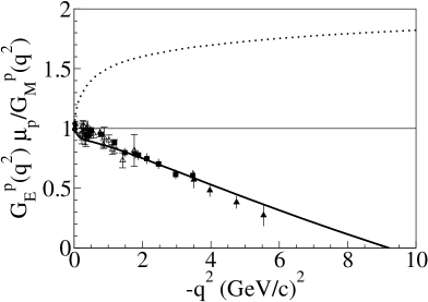
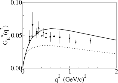
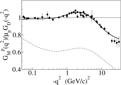
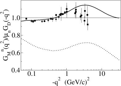
Figure 3: Spacelike nucleon form factors vs $-q^{2}$. Solid lines: full calculation, i.e., sum of triangle plus pair-production terms. Dotted lines: triangle contribution only. Data from the compilations in [20]. $G_{D}(|q^{2}|)=[1+|q^{2}|/(0.71(GeV/c)^{2})]^{-2}$.

   

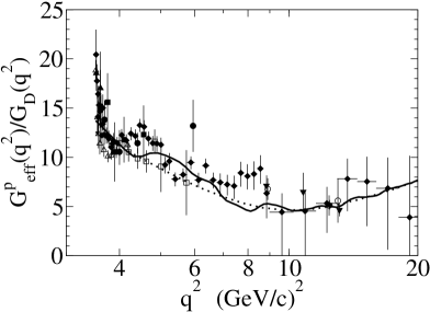
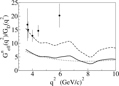
Figure 4: Nucleon effective form factors (see Eq. (13) for the definition) in the timelike region. Solid line: bare + VM. Dotted line: bare term. Left panel: $G^{p}_{eff}(q^{2})/G_{D}(q^{2})$ vs $q^{2}$; data from [21]. Right panel: $G^{n}_{eff}(q^{2})/G_{D}(q^{2})$ vs $q^{2}$; data from [5]. Dashed line: solid line arbitrarily multiplied by 2.

References

[1] I.A. Qattan et al., Phys. Rev. Lett. 94, 142301 (2005), and
references therein quoted.
[2] M.K. Jones et al., Phys. Rev. Lett. 84, 1398 (2000);
O. Gajou et al., Phys. Rev. Lett. 88, 092301 (2002); V. Punjabi et al., Phys. Rev.
C 71, 055202 (2005) and erratum, ibidem, 069902.
[3] S. Kondratyuk, P.G. Blunden, W. Melnitchouk, J.A. Tjon,
Phys. Rev. Lett. 95, 172503 (2005); Y.C. Chen et al., Phys. Rev. Lett.
93, 122301 (2004),
C. E. Carlson, M. Vanderhaeghen, Ann. Rev. Nuc. Part.
Sci. 57, 171 (2007).
[4] Yu.M. Bystritskiy, E.A. Kuraev, E. Tomasi-Gustafsson,
Phys. Rev. C 75, 015207 (2007).
[5] A. Antonelli et al., Nucl. Phys. B 517, 3 (1998).
[6] J. Ellis, M. Karliner, New J. Phys. 4, 18 (2002).
[7] G. A. Miller, arXiv:0802.3731 and references quoted therein.
[9] J. Carbonell, B. Desplanques, V. A. Karmanov,
J. F. Mathiot, Phys. Rep. 300, 215 (1998).
[10]
J.P.B.C. de Melo, T. Frederico, E. Pace and G. Salmè,
Phys. Lett. B 581, 75 (2004); Phys. Rev. D 73, 074013 (2006);
Nucl. Phys.
A 707, 399 (2002); J.P.B.C. de Melo, T. Frederico, E. Pace, G. Salmè
and J. S. Veiga, Proceedings of the Intl. Conf. ”Continuous Advances in QCD
2006”, ed. by M. Peloso and M. Shifman (World Scientific, Singapore, 2007) p.
205, and hep-ph/0609212.
[11] E. Pace, G. Salmè, T. Frederico, S. Pisano
and J.P.B.C. de Melo, Nucl. Phys.
A 782, 69c (2007); A 790, 606c (2007).
[12] W.R.B. de Araújo, E.F. Suisso, T. Frederico, M. Beyer and H.J.
Weber, Phys. Lett. B 478, 86 (2000); Nucl. Phys.
A 694, 351 (2001), and references therein quoted.
[13] F.M. Lev, E. Pace and G. Salmè, Nucl. Phys. A 641, 229
(1998); Phys. Rev. C 62, 064004 (2000).
[14] S. Mandelstam, Proc. Royal Soc. A 233, 248 (1955).
[15] E. Pace, G. Salmè, T. Frederico, S. Pisano and J.P.B.C. de
Melo, to be published.
[16]F. Iachello, A.D. Jackson and A. Lande, Phys. Lett.
B 43, 191 (1973).
[17] W.-M. Yao et al., J. of Phys. G 33, 1 (2006).
[18] T. Frederico, H.-C. Pauli and S.-G. Zhou, Phys. Rev.
D 66, 054007 (2002); Phys. Rev. D 66, 116011 (2002).
[19] M. Cristoforetti, P. Faccioli, G. Ripka and M. Traini,
Phys. Rev. D 71, 114010
(2005).
[20] C. E. Hyde-Wright and K. de Jager, Ann. Rev. Nucl. and Part. Sci. 54, 217 (2004); C.F. Perdrisat, V. Punjabi, M. Vanderhaeghen,
Progr. Part. Nucl. Phys. 59, 694 (2007).
[21] BaBar Collaboration, Phys. Rev. D 73, 012005 (2006), and
references therein quoted.